Spectral flow of fermions in the (anti-)instanton, and the sphaleron with vanishing topological charge
Abstract
The spectral flow is ubiquitous in the physics of soliton-fermion interacting systems. We study the spectral flows related to a continuous deformation of background soliton solutions, which enable us to develop insight into the emergence of fermionic zero modes and the localization mechanism of fermion densities. We investigate a nonlinear sigma model in which there are the (anti-) instantons and also the sphalerons with vanishing topological charge. The standard Yukawa coupling of the fermion successfully generates infinite towers of the spectra and the spectral flow is observed when increasing the size of such solitons. At that moment, the localization of the fermions on the solitons emerges. The avoided crossings are also observed in several stages of the exchange of the flows, they are indicating a manifestation of the fermion exchange of the localizing nature.
I Introduction
Fermion-soliton interacting systems have been extensively investigated in a vast range of physics, including condensed matter physics, particle physics, planetary science and also cosmology. The normalizable modes with zero eigenenergy, the zero modes, certainly develop when fermions interact with soliton solutions [1, 2] 111It depends on the coupling scheme between fermions and solitons. In the fermion-vortex system, for example, the zero mode does not appear in the gauge coupling [3] while it does in the Yukawa coupling [2]., as indicated by the Atiyah-Singer index theorem [4, 5, 6, 7, 8].
The study of the topological solitons has been activated in the context of the fermion-soliton systems. In the kink, localized zero energy fermions and their fractionalization occur [9, 1, 10, 11]. There are the normalizable zero modes in the vortex-fermion system [2, 12], and the ’t Hooft-Polyakov magnetic monopoles [13, 1, 14, 15, 16, 17, 18]. Another non-trivial effect is the nonconservation of the fermion numbers. The instanton in the Yang-Mills theory on four-dimensional Euclidean space [19] has the nontrivial vacuum structure and gives rise to an anomalous phenomenon i.e., the fractionalization of the fermion number and the electric charge [20]. The sphalerons [21, 22] in the Weinberg–Salam theory play a similar role to the instantons, leading to the nontrivial consequence [23].
In the case of the broken time reversal invariance, positive/negative energy eigenvalues of the fermions is asymmetric, which characterizes the spectral asymmetry [24, 25, 6, 26]
where are a tower of energy eigenvalues of fermions. The fermion number in the fermion-soliton system is related to the spectral asymmetry as . The index theorem tells that the fermion number is equal to the topological charge up to the sign, i.e., [6, 26]. The spectral flow of the fermion energy eigenvalues originates from the coincidence.
Numerous details about the number of fermionic zero modes are provided by the index theorem, but it offers less information about the spectral flow, which is a transition in the spectrum with a changing parameter of the soliton in the background. In the instanton or the sphaleron background, rearrangements of energy spectra occur, e.g. one negative energy level undergoes the transition to a positive energy level concerning the imaginary time evolution [23]. Such behavior is commonly referred to as the spectral flow [27, 28, 29], which is a manifestation of the anomaly [30, 27, 31]. In addition to gauge theories, nonlinear sigma models have also been studied [32, 33, 34, 35, 36]. The spectral flow argument is a direct tool for elucidating the connection between topology and flow of the fermions [30, 37, 38, 31, 25].
The bulk-edge correspondences in 2D topological insulators and 3D Weyl semimetals have been extensively studied in a vast number of literature [39, 40, 41, 42]. The spectral flow argument arises at some stages in the research. A more astounding application can be found in the shallow water dynamics of the ocean sea [43, 44].
In this paper, we examine the spectral flow analysis with the nonlinear sigma model. The model possesses two types of analytical solutions: the (anti-)instanton solutions [45], and also the shpalerons, which are non-interacting mixtures of instanton and anti-instanton [46, 47, 48]. There are several possibilities to incorporate the fermionic degrees of freedom into the model, e.g., the minimal coupling [49] and the supersymmetric coupling [50]. In the present paper, we investigate a Yukawa coupling of the Dirac fermions with the instanton and also the sphaleron solutions. These solutions allow us to look at two significant issues. As we mentioned, the normalizable zero-mode solutions are caused by the finite charged topological solitons. Now, we shall study the spectral flow of Dirac fermions interacting with the net-zero topological charged solutions. Another topic is that we shall study the full spectral flow analysis using the moduli parameters of the solutions. In Refs.[51, 52], a size parameter was introduced for realizing the flow of the fermions, which has nothing to do with the solution itself. Another way is that one can employ an interpolating field between the soliton and the vacuum configuration , where the and denotes the soliton and the vacuum configuration [30, 32]. One successfully obtains the normalizable modes, but is only the exact solution at . In terms of the whole range of the moduli parameters of the solutions, we obtain the spectral flow with the true background soliton solutions. As a result, we investigate the sequences of the flows as growing the parameters. At the moment, we ignore any back-reactions from the fermions to the soliton solutions, although the effects could be crucial for the structure of the solitons and also the spectral flows [36, 53, 54, 55].
This paper is organized as follows: In Sec. II, we introduce the solutions of the (anti-)instantons and the sphalerons. The topological charge is defined in this section. Their moduli parameters are described in Sec. II.2. Sec. III is the fermionic model and the details of our numerical method. In Sec. IV, we present the results of the spectral flows for the anti-instanton and the mixture. In Sec. V, we are concentrating on the localization of the fermion density through the avoided crossing. Sec. VI is devoted to our conclusions.
II Nonlinear Sigma Model
A nonlinear sigma model (NLSM) with a target space which is the complex projective space is an important class of quantum field theories [45]. In any , the NLSM has 2D mimic of (anti-) instanton solutions in Yang–Mills gauge theory. Moreover, there are further solutions in that are a non-interacting mixture of instantons and anti-instantons [46, 47, 48], that we simply refer to it as the mixture.
Instantons in -dimensional Euclidean space can be regarded as static topological solitons in dimensions. A model consisting of fermions and instantons can have two different prescriptions. One is that, as utilized in Refs.[56, 37, 31, 25], fermions couple with instantons in a region of space where the instantons localize. Another involves embedding solutions in dimensional spacetime. In this paper, we follow the latter. In the following, we concentrate on the case of the , but the extensions of are straightforward.
II.1 The model and the formal solutions
In this subsection, we provide a formal introduction of the model and its solution. The static energy of the NLSM in -dimensional space-time is given by
| (1) |
where is a three dimensional complex unit vector , and defines a covariant derivative. Since soliton solutions should be of finite energy, the field at the spatial infinity must be a constant vector up to phase. Due to the boundary condition and the identification of : , is compactified to -sphere , and then . The solutions of NLSM are classified by an integer, so-called topological charge , which is defined as
| (2) |
where is an antisymmetric tensor: . In terms of the complex coordinates for convenience, the energy and the topological charge can be rewritten as
| (3) |
| (4) |
with . The equation of motion (EOM) is
| (5) |
From Eq. (3) and Eq. (4), we get
| (6) |
The equality is realized when the solution satisfies the Bogomol’nyi-Prasad-Sommerfield (BPS) equation
| (7) |
The solutions of the equation are referred to as the (anti-)instantons. Their forms can be written in terms of holomorphic vectors
| (8) |
where is -dimensional non-zero holomorphic vectors ( instanton, anti-instanton). The solutions automatically satisfy the BPS equation (7) and also the EOM, and can thus minimize the energy, i.e., . Eqs. (4), (7) tell us that the (anti-)instantons possess a positive (negative) topological charge. Furthermore, a more general class of solutions has been discovered by Din and Zakrzewski, that we refer to it as Din–Zakrzewski (DZ) solutions [46, 47, 48]. Using the Bäcklund transformation
| (9) |
with , the DZ solutions are obtained as
| (10) |
Note that s are independent solutions of the EOM (5) for each . One can verify that only and satisfy the BPS equation, i.e., and . This means that has positive, and has negative topological charge. Therefore, they are instanton and anti-instanton solutions respectively. Generally, the other solution, , does not satisfy the BPS equation. From Eq. (6), we can see that if satisfies the BPS equation (7), the energy is minimized, whereas if it does not, the energy is higher. Therefore, such a non-BPS solution is a saddle point for the energy. As we see later, it can be interpreted as a mixture solution of instantons and anti-instantons.
Since there are three types of the solutions in the NLSM. For all solutions, we give formal forms of the energy, the topological charge, and their densities
| (11) | ||||
| (12) |
The and are the solutions of the BPS equation, but the is not. More explicit form of the energy densities and the topological charge densities are given as
| (13) | ||||
| (14) |
From these, one directly checks that the energy and the topological charge of the instanton and the anti-instanton have the connection and . Also, after some algebra (see the Appendix A), we can confirm that the components of and can be written as
| (15) |
As a result, the energy and the topological charge have the form below:
| (16) | ||||
| (17) |
From these, can be interpreted as a non-interacting composite of the instantons and the anti-instantons. Therefore, we call the solution as the mixture. Since and are the positive and negative part of the topological charge of the mixture, then the anti-instanton and the instanton are the instanton and anti-instanton part of the mixture, respectively. To make the meaning more clear, we rewrite to which stand for the instanton, the mixture, and the anti-instanton solutions, respectively. Accordingly, the energy, the topological charges and the densities are now , , and .
II.2 The explicit solutions
In this subsection, we construct the explicit DZ solutions in the NLSM, with introducing the parameters which govern the deformation of solutions. We employ a simple holomorphic vector
| (18) |
where denote polar coordinates defined through and are generally complex constants. Here we note that thanks to global symmetry of the model (3), they are set to be non-negative real numbers without loss of generality. For the boundary conditions imposed on the soliton solutions, the finiteness of is required.
By the nonlinear operator acting on , we obtain the DZ solutions as followings:
| (19) | ||||
| (20) | ||||
| (21) |
where are defined by
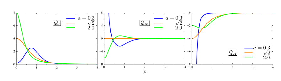
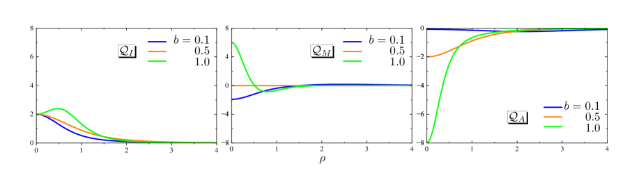
Here we emphasize that, for arbitrary parameters , , and are exact solutions of EOM (5). We designate Eq.(19)–Eq.(21) as axially symmetric solutions because the topological charge densities and energy densities evaluated by (19)–(21) are the function of the radial coordinate .
| The parameters | |||
|---|---|---|---|
The topological charge densities can be written as
| (22) | ||||
| (23) | ||||
| (24) |
After the integration, we obtain the topological charges
| (25) |
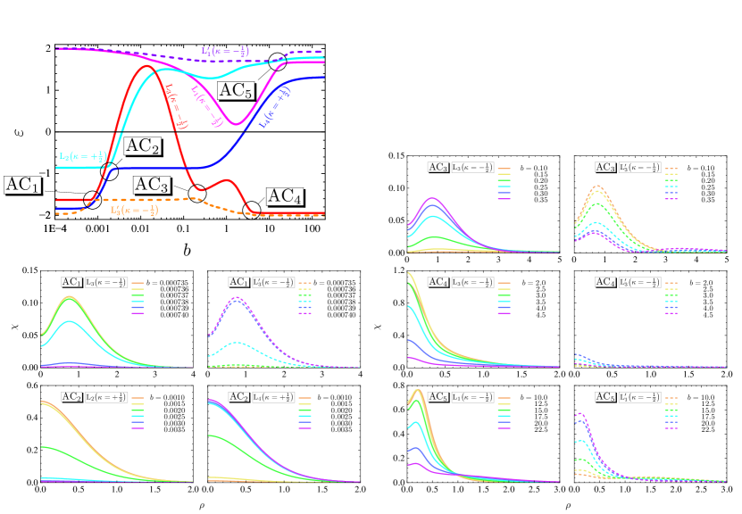
which is supported for all the parameters choice . It should be emphasized that we obtain completely different values for the topological charges when we use the limiting values of the parameters, such as . The results are summarized in Table. 1. As a result, the deformations of the solutions successfully induce the spectral flow since the DZ solutions (19)-(21) are the function of the parameters. For example, a parameter sequence with finite of the anti-instanton corresponds to a transition of the anti-instanton charge , that certainly causes the two levels to cross the zero energy line as grows.
III Fermionic sigma model
We consider the fermions coupled with the DZ solutions that are embedded into dimensional spacetime.
III.1 The Effective Action and the NLSM
For the construction of the model, we begin with a partition function defined in three dimensional Euclidean space
| (26) |
where is called a Dirac operator. Here is a coupling constant and the gamma matrices are given by the standard Clifford algebra
| (27) |
In the two space dimensions, the matrices are given by and where are the standard Pauli matrices. For the spectral flow analysis of the DZ solutions, we provide an efficient Yukawa-type coupling with a nice parametrization of in terms of a matrix-valued field , i.e., the principal variable. [57, 58]. Formally, it is defined by
| (28) |
It parametrizes the coset space with the subgroup being invariant under the involutive automorphism . It follows that for . The model possesses some symmetries. With the definition (28), one finds that the principal variable possesses the following property
| (29) |
The low-energy effective action of this theory includes the aforementioned NLSM, which can be derived using a perturbative method. Here, we give a brief outline of the derivation using a normal derivative expansion [59, 60]. Integrating out the fermion fields in the partition function , we obtain so-called a Dirac determinant
| (30) |
Therefore, is now
| (31) |
where is called the effective action. is not Hermitian in Euclidean space, so we separate into the real part and the imaginary part, and each component becomes
| (32) | ||||
| (33) |
where means a functional trace taking all trace, i.e. matrices, states, and Euclidean space. Using a derivative expansion, we can evaluate the regularized real part of the action leaving only the first nonzero orders in as
| (34) |
Note that the principal variable has directly related to , 222Through this representation, the principal variable has another direct connection with the color field , such that . For more general case of , this kind of connection holds. such as
From this, we confirm that the action (34) becomes
| (35) |
where is exactly the energy functional in the NLSM. Since the background field is independent of , the terms with imaginary time derivatives vanish. We can evaluate the imaginary part of the action in a similar fashion, which often contains the imaginary time derivative, and always vanishes in our model.
III.2 The Dirac Hamiltonian and Method for the Computation
For the spectral flow analysis, we numerically solve an eigenequation of the Dirac Hamiltonian
| (36) |
The Hamiltonian is derived from the Dirac operator
| (37) |
The explicit form of the Hamiltonian is (a) (b) Fig. 3: The spectral flow of the anti-instanton solution. (a) The flow with change of the parameter , and (b) of the parameter .
![[Uncaptioned image]](/html/2403.10149/assets/x3.png)
![[Uncaptioned image]](/html/2403.10149/assets/x4.png)
(a) (b) Fig. 4: The spectral flow of the mixture solution. (a) The flow with change of the parameter , and (b) of the parameter .
We solve the Dirac eigenequation (36) corresponding to the Hamiltonian (LABEL:hamiltonian) numerically. Since the Hamiltonian depends on the parameters through the , we can analyze the spectral flow of the fermions as a function of .
Here we provide a quick overview of the procedure that is being developed in Ref.[61]. The secular equation for the energy eigenvalue is given by
| (39) |
where the matrix element of and is given by
| (40) | ||||
| (41) |
To obtain these matrix representations, we construct plane-wave spinor bases which are the eigenvectors of the Hamiltonian of the massive free fermions . They are given by
| (42) | ||||
| (43) | ||||
| (44) |
where are standard Bessel functions with the integer order . The coefficients are given by
where are the vacuum energy eigenvalues.
We can construct the bases in a cylinder of radius . This radius is ideally infinite, however, for numerical computation, it must take a finite value. Imposing boundary conditions
| (45) |
for , we obtain some sets of discretized wave numbers . The orthogonality conditions are given by
| (46) |
Then, the normalization constants are determined as
| (47) |
In this setup, the plane waves form orthonormal bases.
By solving the secular equation (39) numerically for each parameter , we can obtain some energy spectra and corresponding wave functions for each . The eigenproblem (39) is solved by a standard matrix diagonalization solver ’dsyev’ in the LAPACK, Math Kernel Library. Note that to study the localization of wave functions to the background soliton in real space, we calculate the fermion density which is defined by
| (48) |
In Sec. V, we shall see property of the localization of is strongly linked to the spectral flow. For our numerical computations, we set and the number of discrete wavenumbers is chosen as , which gives a sufficient convergence.
IV Results: the spectral flow
Many previous studies on spectral flow analysis have shown the level crossings in which the background fields do not represent the solution of the model [51, 52, 30, 32]. One of the characteristic features of this study is that the background field is always the solution of the equation of motion, because of the spectral flow with the moduli parameters . Since changing causes expansions or deformations of the solutions (see Fig. 1 and Fig. 2), it is possible to derive the spectral flow as a function of these moduli parameters. As the spectral flow analysis with the instanton solutions was previously discussed in Ref.[33], here we concentrate on the results of the anti-instanton and the mixture solution.
Fig.III.2 plots the behavior of the energy spectra for the anti-instantons with the parameters change. First, we begin by analyzing the result of varying shown in Fig.III.2(a). The topological charge at and the background field is a vacuum solution; The number of positive and negative energy levels is strictly equal, as indicating the fermion number . The topological charge switches on for . As gradually increasing the parameter , the two energy levels (colored in magenta and cyan) move from the positive continuum to the negative. As a result, the number of positive levels decreases and negative rises by respectively, which corresponds to , and then . Note that and are not necessarily correlated with each other. We see the local behavior of the energy levels of the regions I – V in Fig.III.2(a). From region I to II, the positive level decreases and the negative increases by 1 which corresponds to the change of . From region II to III, the additional level comes from positive to negative, that is is now . As a result, the number of zero modes ( the number of crossing zero energy lines) between regions I and III equals to . For larger , since the topological charge continues to be as shown in Table. 1, it is expected that no further net crossing can appear. Actually, in Fig. III.2(a), one can confirm that the sign flip of the energy levels does not occur at large .
It is worth discussing the behavior of the soliton at the vicinity of . As it was already utilized in previous analysis [62, 51, 52], the solitons with tiny size do not induce the fermion number at all. The situation is comparable to the bound state problem in the quantum mechanical potential well [63], when a bound state is absent below a certain threshold for the potential’s size or depth. Therefore, the solution with sufficiently small has the same effect as the vacuum configuration.
In the case with the parameter (Fig.III.2(b), more complex behavior emerges. Given that the series passes over , there needs to be one more crossing zero energy. The magenta level descends and after that, it returns to the positive continuum. The transition of the topological charge appropriately results in this swing- back behavior, and the spectral flow appropriately connects the fermion number .
Next, we discuss the spectral flow for the mixture, sphaleron solution . This solution has zero net topological charge since it appears to composite two instantons and two anti-instantons. As we showed in Table 1, it behaves as (anti-) instantons at some parameter limits. Therefore, the spectral flow connects three different states: the anti-instanton, the mixture, and the instanton. As you can see in Fig.III.2, four zero modes manifest in the process of the spectral flows. We begin with the change of in Fig.III.2(a). With the topological charge is , meaning that there are two more negative energy levels than there are in the vacuum state. As increasing , the magenta levels and the cyan cross the zero-energy line from negative to positive, corresponding to the change of . In region III, the number of negative levels and the positive levels are equal, i.e., , and the energy gap between them significantly decreases, there is a nontrivial modulation to the vacuum. Further increasing , additional two levels, the red and the blue move from negative to positive, which corresponds to the change of . In region V, the charge finally arrives at . Since the topological charge changes from to , the four zero modes manifest in the process of the spectral flow.
As one can see in Fig.III.2(b), again the behavior for the change of the parameter is a little more complex. The red level crosses the zero-energy line once and then crosses it again and goes back to the negative as growing . In region I, the number of negative levels has increased by one. As increasing , the red and cyan levels move from negative to positive, with the change of : . A larger , the red level crosses the zero-energy line again, and the blue level moves from negative to positive, corresponding to : . In this process, the energy spectra cross the zero-energy line a total of four times, indicating the existence of four zero modes. However, the red level undergoes an even number of crossings, resulting in net two crossings over the entire spectral flow.
In conclusion, we obtain a firm result regarding the complete correlation among the number of zero modes in all ranges of the parameters , the number of crossings of the zero energy line, and the change of or . The net number of crossings equals the difference in topological charges at the parameter limits. On the other hand, the number of zero modes is not necessarily equivalent to them as seen in Fig.III.2(b) and Fig.III.2(b). To fix the exact number of the zero modes, we just count the number of times the fermion number changes. The spectral flow analysis is the best way to do this.
V Results: The localizing Fermions
The localizing Dirac fermions coupled with the texture-type topological soliton (i.e.,the skyrmion) were first addressed in Refs.[51, 52]. The zero modes of fermions are localized on a linear profile function: of sufficiently large size . We stress once more that they do not represent the solutions on the genuine background profile. In this section, we present the true localizing solutions on the genuine solitons.
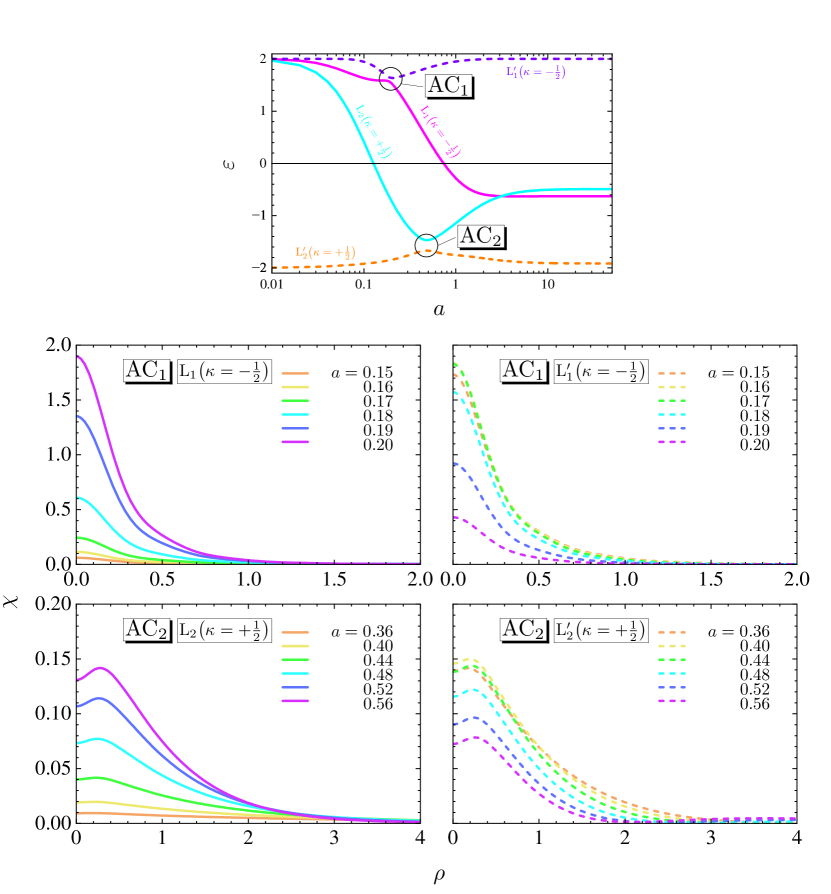
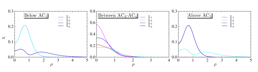
First, we consider the case of the anti-instanton. At the vacuum, occurs with or (see Table. 1), and the fermions are not localized. As increasing the parameters , the localization emerges. It is an intricate process that is often triggered by the energy level junction, which is also referred to as an energy level repulsion or an avoided crossing (AC). Fig. 5 shows the spectral flow and the fermion densities of varying for the anti-instanton. The levels concerning the avoided crossing are Li, L, and they are situated at AC1 and AC2. On the junctions, the localization property is exchanged with each other. For example, at around the AC1, below the density of L is localized, while the L1 is not. The L density starts to delocalize and the L1 density localizes at . The same has happened at the AC2.
In Fig. 6, the spectral flow for the change of is plotted and, one can see some ACs. The L1,L2 are the delocalized mode at . They transition into localized modes via the AC1 at . It is a almost similar behavior as the previous one, but now the level L1 again encounters the next ACs, interaction between levels L1 and L occurs at . Now the localization of the L1 transitions to the counterpart L. The L is to be a continuous mode in the limit of , by the additional AC with the other continuous levels. Since the L2 remains a discrete level for the whole . Consequently, only the density of L2 remains as the localizing mode for large, that is, .
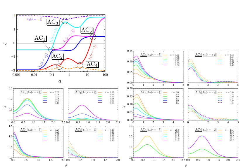
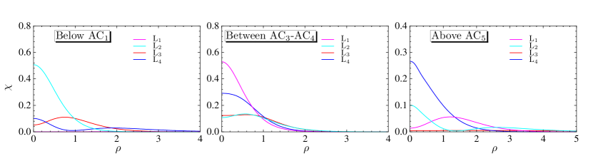
Our new insights into the fermion density localization are effective for understanding the case of the mixture solution. Fig. 7 shows the spectral flow of the mixture and the corresponding fermion density as is varied. The four levels move from negative to positive as grows, and the five ACs switch their localization and delocalization. This results in the localization of L1 and L2 densities in the region where is small, and of L3 and L4 densities in the region where is large. Recalling that the mixture behaves as the anti-instanton where is sufficiently small and as the instanton where is sufficiently large, one can see that the L1 and L2 densities are modes localized in the anti-instanton part of the mixture, and the L3 and L4 densities in the instanton part. Here, the behavior of the fermion density around gives us a deep understanding of the mixture solution. In the region, the four fermion densities are localized as shown in Fig. 8. Consequently, the modes localized in the anti-instanton component and the instanton part coexist in this region. This means that the mixture with topological charge is not just a topologically trivial field, but has the function of trapping fermions and closing the energy gap as discussed in the previous section. Moreover, we can interpret fermions can detect the instantons and anti-instantons inside the mixture.
The (de)localization of fermion densities occur by the same mechanism in the spectral flow when is varied, as shown in Fig. 9 and Fig. 10. Since the level L3 crosses the zero-energy line an even number of times, the switching between localized and delocalized state occurs more than once (totally three times), as explained in the anti-instanton case.
VI Conclusions
In this paper, we developed a novel approach to the realization of spectral flows pertaining to solitons’ parameters in the NLSM. We elucidated the connection between fermion density localization and the emergence of the fermion zero mode. Since the (anti-)instantons and the mixtures are the exact solutions with the two moduli parameters, our spectral flow analysis meaningful for the whole parameter space. At the spectral flow, some energy levels cross zero and the net number of the crossings coincides with the difference of topological charge of both ends of the flow. In the previous studies concerning the spectral flow, they claimed that the number of crossings should be equivalent to the number of zero modes. In this paper, we examined the flows between the solutions with the several charges, so the number of zero modes reflect how many times the topological charge changes its value.
The solutions consist of the anti-instanton (), the mixture () and the instanton (). The spectral flow analysis for the mixture is one of the most intriguing results. The energy gap closes in the region, indicating that the mixture realizes an instanton + anti-instanton composite with an interior structure rather than just being a topologically trivial one.
For the localization property of the fermions, generally, a large soliton solution induces the localizing fermion mode. It is also essential that the transition between localizing and delocalizing fermion density is observed. The avoided crossings between relevant energy levels play a role in such transition of the fermion density. In other words, it is concluded that the localization of the fermion density depends not only on the soliton size but also on the presence of AC in the spectral flow. The localization also occurs in the spectral flow of the mixture solution. Of particular interest is the fact that the four fermion densities are localized in the region , containing both the instanton-localized and the anti-instanton-localized densities. This result implies that the fermions can successfully detect the (anti-) instanton inside the mixture.
Our spectral flow analysis, utilizing parameters of the solutions, has provided two crucial outcomes:
-
1.
The spectral asymmetry,
-
2.
The (de)localization of density of the fermions.
Both are deeply intertwined with the topology through the index theorem. The former emerges as a manifestation of the global change of the topology, represented by the difference in topological charges at the outside of the parameter space. (see Sec.V). On another hand, the latter has a more geometrical origin; it often arises through the avoided crossings in the spectral flow process. It is worth repeating that we were able to discuss the second property since the spectral flow was treated exactly. Since topology signifies a solitonic symmetry, the avoided crossings indicate signs of subtle modulation of the symmetry. Therefore, it is envisaged that the avoided crossings arising in the spectrum flow will serve as a harbor for new physics in the fermion-soliton system. As case studies, the avoided crossings could be explored in systems such as the flag manifold sigma model [64, 65, 66, 67], an extension of the NLSM to large homotopy group, or composite soliton systems such as domain-wall skyrmion chain [68]. We will report on these issues in our subsequent papers.
Acknowledgement
The authors would like to thank P.Klimas, Y.Shnir, F.Blaschke, F.Hanada, A.Nakamula and K.Toda for their many usefull comments. Y.A. was supported in part by JSPS KAKENHI Grant Number JP23KJ1881. N.S. was supported in part by JSPS KAKENHI Grant Number JP20K03278, and also JP23K02794.
Appendix A Derivation of the mixed charge or energy density
In this appendix, we derive the topological charge or energy density of a mixture in terms of the ( anti-) instanton charge density and or energy density and . We use the following properties without proof:
| (49) | |||
| (50) |
The first one can be verified recursively, and one can directly see that the second one is automatically satisfied for an arbitrary .
Let us define a Bäcklund transformation:
| (51) | ||||
| (52) |
This definition leads a relation, for an arbitrary . Therefore, the topological charge densities have the form below:
| (53) | ||||
| (54) | ||||
| (55) |
In the same way, the energy densities have the form below:
| (56) | ||||
| (57) | ||||
| (58) |
Our goal is to derive two relations:
| (59) | ||||
| (60) |
These relations lead and .
A.1 Instanton part
In this subsection, we show
| (61) |
In order to see this, we calculate
| (62) |
The second term of Eq. (62) vanishes because of ,
| (63) |
Thus we obtain
| (64) |
Here we consider . Then, has the form
| (65) |
and we have
| (66) |
Therefore, we obtain
| (67) |
A.2 Anti-instanton part
In this subsection, we show
| (68) |
The method is the same as for the instanton part. We calculate
| (69) |
The second term of Eq. (69) vanishes because of . First, we show this fact. The main component can be reduced into
| (70) |
Since we have
| (71) |
from Eq. (64), the component of the third term of Eq. (70) has the form
| (72) |
And the component of the second term of Eq. (70) is
| (73) |
As a result, Eq. (70) can be written as follows:
| (74) |
Here using a relation
| (75) |
Eq. (74) has a more simple form,
| (76) |
Recalling that does not contain (see Eq. (72) and ), the second term of Eq. (69) vanishes, i.e.
| (77) |
Therefore we obtain
| (78) |
From Eq. (72), the first term of Eq. (78) is
| (79) |
Considering
| (80) |
Eq. (78) can be written as
| (81) |
and then we have
| (82) |
Therefore, we obtain the relation
| (83) |
References
- Jackiw and Rebbi [1976] R. Jackiw and C. Rebbi, Solitons with Fermion Number 1/2, Phys. Rev. D 13, 3398 (1976).
- Jackiw and Rossi [1981] R. Jackiw and P. Rossi, Zero Modes of the Vortex - Fermion System, Nucl. Phys. B 190, 681 (1981).
- de Vega [1978] H. J. de Vega, Fermions and Vortex Solutions in Abelian and Nonabelian Gauge Theories, Phys. Rev. D 18, 2932 (1978).
- Atiyah and Singer [1969] M. F. Atiyah and I. M. Singer, The index of elliptic operators on compact manifolds, Bull. Am. Math. Soc. 69, 422 (1969).
- Atiyah et al. [1975] M. F. Atiyah, V. K. Patodi, and I. M. Singer, Spectral asymmetry and riemannian geometry. i, Mathematical Proceedings of the Cambridge Philosophical Society 77, 43–69 (1975).
- Niemi and Semenoff [1984] A. J. Niemi and G. W. Semenoff, Spectral asymmetry on an open space, Phys. Rev. D 30, 809 (1984).
- Anghel [1989] N. Anghel, Remark on callias’ index theorem, Reports on Mathematical Physics 28, 1 (1989).
- Bott and Seeley [1978] R. Bott and R. Seeley, Some remarks on the paper of Callias: “Axial anomalies and index theorems on open spaces”, Communications in Mathematical Physics 62, 235 (1978).
- Dashen et al. [1974a] R. F. Dashen, B. Hasslacher, and A. Neveu, Nonperturbative Methods and Extended Hadron Models in Field Theory 2. Two-Dimensional Models and Extended Hadrons, Phys. Rev. D 10, 4130 (1974a).
- Klimashonok et al. [2019] V. Klimashonok, I. Perapechka, and Y. Shnir, Fermions on kinks revisited, Phys. Rev. D 100, 105003 (2019).
- Perapechka and Shnir [2020] I. Perapechka and Y. Shnir, Kinks bounded by fermions, Phys. Rev. D 101, 021701 (2020).
- Weinberg [1981] E. J. Weinberg, Index Calculations for the Fermion-Vortex System, Phys. Rev. D 24, 2669 (1981).
- Dashen et al. [1974b] R. F. Dashen, B. Hasslacher, and A. Neveu, Nonperturbative Methods and Extended Hadron Models in Field Theory. 3. Four-Dimensional Nonabelian Models, Phys. Rev. D 10, 4138 (1974b).
- Callan [1983] C. G. Callan, Jr., Monopole Catalysis of Baryon Decay, Nucl. Phys. B 212, 391 (1983).
- Rubakov [1982] V. A. Rubakov, Adler-Bell-Jackiw Anomaly and Fermion Number Breaking in the Presence of a Magnetic Monopole, Nucl. Phys. B 203, 311 (1982).
- Rubakov [1988] V. A. Rubakov, Monopole Catalysis of Proton Decay, Rept. Prog. Phys. 51, 189 (1988).
- Brennan [2023] T. D. Brennan, Callan-Rubakov effect and higher charge monopoles, JHEP 02, 159, arXiv:2109.11207 [hep-th] .
- Brennan [2022] T. D. Brennan, Index-like theorem for massless fermions in spherically symmetric monopole backgrounds, JHEP 03, 095, arXiv:2106.13820 [hep-th] .
- Belavin et al. [1975] A. Belavin, A. Polyakov, A. Schwartz, and Y. Tyupkin, Pseudoparticle solutions of the yang-mills equations, Physics Letters B 59, 85 (1975).
- Jackiw and Rebbi [1977] R. Jackiw and C. Rebbi, Spinor Analysis of Yang-Mills Theory, Phys. Rev. D 16, 1052 (1977).
- Klinkhamer and Manton [1984] F. R. Klinkhamer and N. S. Manton, A Saddle Point Solution in the Weinberg-Salam Theory, Phys. Rev. D 30, 2212 (1984).
- Manton and Sutcliffe [2004] N. S. Manton and P. Sutcliffe, Topological solitons, Cambridge Monographs on Mathematical Physics (Cambridge University Press, 2004).
- Kunz and Brihaye [1994] J. Kunz and Y. Brihaye, Level crossing along sphaleron barriers, Phys. Rev. D 50, 1051 (1994), arXiv:hep-ph/9403216 .
- Niemi [1985a] A. J. Niemi, Spectral Density and a Family of Dirac Operators, Nucl. Phys. B 253, 14 (1985a).
- Niemi and Semenoff [1986] A. J. Niemi and G. W. Semenoff, Fermion Number Fractionization in Quantum Field Theory, Phys. Rept. 135, 99 (1986).
- Niemi and Semenoff [1983] A. J. Niemi and G. W. Semenoff, Axial-anomaly-induced fermion fractionization and effective gauge-theory actions in odd-dimensional space-times, Phys. Rev. Lett. 51, 2077 (1983).
- Witten [2016] E. Witten, Fermion Path Integrals And Topological Phases, Rev. Mod. Phys. 88, 035001 (2016), arXiv:1508.04715 [cond-mat.mes-hall] .
- Manton [1985] N. Manton, The schwinger model and its axial anomaly, Annals of Physics 159, 220 (1985).
- Alkofer and Reinhardt [1995] R. Alkofer and H. Reinhardt, Chiral quark dynamics, Vol. 33 (1995).
- Witten [1982] E. Witten, An SU(2) Anomaly, Phys. Lett. B 117, 324 (1982).
- Niemi and Semenoff [1985] A. J. Niemi and G. W. Semenoff, Spectral Flow and the Anomalous Production of Fermions in Odd Dimensions, Phys. Rev. Lett. 54, 873 (1985).
- Amari et al. [2019a] Y. Amari, M. Iida, and N. Sawado, Statistical Nature of Skyrme-Faddeev Models in 2+1 Dimensions and Normalizable Fermions, Theor. Math. Phys. 200, 1253 (2019a), arXiv:1910.10431 [hep-th] .
- Amari et al. [2023] Y. Amari, N. Sawado, and S. Yamamoto, Instanton size dependence on fermion energy spectra in a P2 fermionic sigma model, J. Phys. Conf. Ser. 2667, 012024 (2023).
- Delsate and Sawado [2012] T. Delsate and N. Sawado, Localizing modes of massive fermions and a U(1) gauge field in the inflating baby-skyrmion branes, Phys. Rev. D 85, 065025 (2012), arXiv:1112.2714 [gr-qc] .
- Kodama et al. [2009] Y. Kodama, K. Kokubu, and N. Sawado, Localization of massive fermions on the baby-skyrmion branes in 6 dimensions, Phys. Rev. D 79, 065024 (2009), arXiv:0812.2638 [hep-th] .
- Perapechka et al. [2018] I. Perapechka, N. Sawado, and Y. Shnir, Soliton solutions of the fermion-Skyrmion system in (2+1) dimensions, JHEP 10, 081, arXiv:1808.07787 [hep-th] .
- Burnier [2006] Y. Burnier, Anomalous fermion number nonconservation: Paradoxes in the level crossing picture, Phys. Rev. D 74, 105013 (2006), arXiv:hep-ph/0609028 .
- Weinberg [2012] E. J. Weinberg, Classical solutions in quantum field theory: Solitons and Instantons in High Energy Physics, Cambridge Monographs on Mathematical Physics (Cambridge University Press, 2012).
- Hasan and Kane [2010] M. Z. Hasan and C. L. Kane, Topological Insulators, Rev. Mod. Phys. 82, 3045 (2010), arXiv:1002.3895 [cond-mat.mes-hall] .
- Yu et al. [2017] Y. Yu, Y.-S. Wu, and X. Xie, Bulk–edge correspondence, spectral flow and atiyah–patodi–singer theorem for the z2-invariant in topological insulators, Nuclear Physics B 916, 550 (2017).
- Teo and Kane [2010] J. C. Y. Teo and C. L. Kane, Topological Defects and Gapless Modes in Insulators and Superconductors, Phys. Rev. B 82, 115120 (2010), arXiv:1006.0690 [cond-mat.mes-hall] .
- Fu and Kane [2008] L. Fu and C. L. Kane, Superconducting Proximity Effect and Majorana Fermions at the Surface of a Topological Insulator, Phys. Rev. Lett. 100, 096407 (2008), arXiv:0707.1692 [cond-mat.mes-hall] .
- Delplace et al. [2017] P. Delplace, J. B. Marston, and A. Venaille, Topological origin of equatorial waves, Science 358, 1075 (2017).
- Tauber and Thiang [2023] C. Tauber and G. Thiang, Topology in shallow-water waves: A spectral flow perspective, Annales Henri Poincaré 24, 107 (2023).
- D’Adda et al. [1978] A. D’Adda, M. Luscher, and P. Di Vecchia, A 1/n Expandable Series of Nonlinear Sigma Models with Instantons, Nucl. Phys. B 146, 63 (1978).
- Din and Zakrzewski [1980a] A. M. Din and W. J. Zakrzewski, General Classical Solutions in the CP(n-1) Model, Nucl. Phys. B 174, 397 (1980a).
- Din and Zakrzewski [1980b] A. M. Din and W. J. Zakrzewski, Properties of General Classical CP(n-1) Solutions, Phys. Lett. B 95, 419 (1980b).
- Din and Zakrzewski [1981a] A. M. Din and W. J. Zakrzewski, Interpretation and Further Properties of General Classical CP(n-1) Solutions, Nucl. Phys. B 182, 151 (1981a).
- Din and Zakrzewski [1982] A. M. Din and W. J. Zakrzewski, DECOUPLING IN CP**(n-1) MODELS WITH FERMIONS, Nuovo Cim. A 72, 214 (1982).
- Din and Zakrzewski [1981b] A. Din and W. Zakrzewski, Fermion solutions in the supersymmetric cpn-1 model, Physics Letters B 101, 166 (1981b).
- Kahana and Ripka [1984] S. Kahana and G. Ripka, Baryon Density of Quarks Coupled to a Chiral Field, Nucl. Phys. A 429, 462 (1984).
- Kahana et al. [1984] S. Kahana, G. Ripka, and V. Soni, Soliton with Valence Quarks in the Chiral Invariant Sigma Model, Nucl. Phys. A 415, 351 (1984).
- Perapechka and Shnir [2019] I. Perapechka and Y. Shnir, Fermion exchange interaction between magnetic Skyrmions, Phys. Rev. D 99, 125001 (2019), arXiv:1901.06925 [hep-th] .
- Loginov [2023] A. Y. Loginov, Fermion scattering on topological solitons in the CPN-1 model, Phys. Rev. D 107, 065011 (2023), arXiv:2301.12425 [hep-th] .
- Loginov [2024] A. Y. Loginov, Fermion-soliton scattering in a modified model, (2024), arXiv:2402.02422 [hep-th] .
- Kiskis [1978] J. E. Kiskis, Fermion Zero Modes and Level Crossing, Phys. Rev. D 18, 3690 (1978).
- Eichenherr and Forger [1980] H. Eichenherr and M. Forger, More about non-linear sigma models on symmetric spaces, Nucl. Phys. B 164, 528 (1980), [Erratum: Nucl.Phys.B 282, 745–745 (1987)].
- Ferreira and Klimas [2010] L. A. Ferreira and P. Klimas, Exact vortex solutions in a Skyrme-Faddeev type model, JHEP 10, 008, arXiv:1007.1667 [hep-th] .
- Diakonov et al. [1988] D. Diakonov, V. Y. Petrov, and P. V. Pobylitsa, A Chiral Theory of Nucleons, Nucl. Phys. B 306, 809 (1988).
- Abanov and Wiegmann [2000] A. G. Abanov and P. B. Wiegmann, Theta terms in nonlinear sigma models, Nucl. Phys. B 570, 685 (2000), arXiv:hep-th/9911025 .
- Amari et al. [2019b] Y. Amari, M. Iida, and N. Sawado, Level crossing of fermions coupled with the PN Skyrme-Faddeev model, J. Phys. Conf. Ser. 1194, 012004 (2019b).
- Niemi [1985b] A. J. Niemi, Relation between the spin and the size of a skyrmion, Phys. Rev. Lett. 54, 631 (1985b).
- Landau and Lifshitz [1981] L. Landau and E. Lifshitz, Quantum Mechanics: Non-Relativistic Theory, Vol. 3 (Elsevier, 1981).
- Amari and Sawado [2018a] Y. Amari and N. Sawado, SU(3) knot solitons: Hopfions in the F2 Skyrme–Faddeev–Niemi model, Physics Letters B 784, 294 (2018a).
- Amari and Sawado [2018b] Y. Amari and N. Sawado, Bps sphalerons in the nonlinear sigma model, Phys. Rev. D 97, 065012 (2018b).
- Bykov [2016] D. Bykov, Classical solutions of a flag manifold -model, Nucl. Phys. B 902, 292 (2016), arXiv:1506.08156 [hep-th] .
- Kobayashi et al. [2021] R. Kobayashi, Y. Lee, K. Shiozaki, and Y. Tanizaki, Topological terms of (2+1)d flag-manifold sigma models, JHEP 08, 075, arXiv:2103.05035 [hep-th] .
- Gudnason and Nitta [2014] S. B. Gudnason and M. Nitta, Domain wall skyrmions, Phys. Rev. D 89, 085022 (2014).