Towards Adversarially Robust Dataset Distillation by Curvature Regularization

Abstract

Dataset distillation (DD) allows datasets to be distilled to fractions of their original size while preserving the rich distributional information so that models trained on the distilled datasets can achieve a comparable accuracy while saving significant computational loads. Recent research in this area has been focusing on improving the accuracy of models trained on distilled datasets. In this paper, we aim to explore a new perspective of DD. We study how to embed adversarial robustness in distilled datasets, so that models trained on these datasets maintain the high accuracy and meanwhile acquire better adversarial robustness. We propose a new method that achieves this goal by incorporating curvature regularization into the distillation process with much less computational overhead than standard adversarial training. Extensive empirical experiments suggest that our method not only outperforms standard adversarial training on both accuracy and robustness with less computation overhead but is also capable of generating robust distilled datasets that can withstand various adversarial attacks.

1 Introduction

In the era of big data, the computational demands for training deep learning models are continuously growing due to the increasing volume of data. This presents substantial challenges, particularly for entities with limited computational resources. To mitigate such issues, concepts like dataset distillation (Wang et al., 2018) and dataset condensation (Zhao et al., 2021; Zhao and Bilen, 2021, 2023) have emerged, offering a means to reduce the size of the data while maintaining its utility. A successful implementation of dataset distillation can bring many benefits, such as enabling more cost-effective research on large datasets and models.

Dataset distillation refers to the task of synthesizing a smaller dataset such that models trained on this smaller set yield high performance when tested against the original, larger dataset. The dataset distillation algorithm takes a large dataset as input and generates a compact, synthetic dataset. The efficacy of the distilled dataset is assessed by evaluating models trained on it against the original dataset.

Conventionally, distilled datasets are evaluated based on their standard test accuracy. Therefore, recent research has expanded rapidly in the direction of improving the test accuracy following the evaluation procedure (Sachdeva and McAuley, 2023). Additionally, many studies focus on improving the efficiency of the distillation process (Sachdeva and McAuley, 2023).

Less attention, however, has been given to an equally important aspect of this area of research: the adversarial robustness of models trained on distilled datasets. Adversarial robustness is a key indicator of a model’s resilience against malicious inputs, making it a crucial aspect of trustworthy machine learning. Given the potential of dataset distillation to safeguard the privacy of the original dataset (Geng et al., 2023; Chen et al., 2023), exploring its capability to also enhance model robustness opens a promising avenue for advancing research in trustworthy machine learning (Liu et al., 2023a).

Thus, our work seeks to bridge this gap and focuses on the following question: How can we embed adversarial robustness into the dataset distillation process, thereby generating datasets that lead to more robust models? Motivated by this question, we explore potential methods to accomplish this goal. As it turns out, it is not as simple as adding adversarial training to the distillation process. To find a more consistent method, we study the theoretical connection between adversarial robustness and dataset distillation. Our theory suggests that we can directly improve the robustness of the distilled dataset by minimizing the curvature of the loss function with respect to the real data. Based on our findings, we propose a novel method, GUARD (Geometric regUlarization for Adversarial Robust Dataset), which incorporates curvature regularization into the distillation process. We then evaluate GUARD against existing distillation methods on ImageNette, Tiny ImageNet, and ImageNet datasets. In summary, the contributions of this paper are as follows

• Empirical and theoretical exploration of adversarial robustness in distilled datasets

• A theory-motivated method, GUARD, that offers robust dataset distillation with minimal computational overhead

• Detailed evaluation of GUARD to demonstrate its effectiveness across multiple aspects

The remainder of this paper is structured as follows. In Section 2, we introduce a range of related works that provide context for our research. In Section 3, we offer a background to our study with a concise overview of dataset distillation, some preliminary results, and a formulation of the robust dataset distillation problem. In Section 4, we first explore the theoretical connections between dataset distillation and adversarial robustness, and then introduce the method, GUARD, based on our findings. The experiment results and discussions are subsequently detailed in Section 5 and Section 6, and we conclude the paper with a summary in Section 7.

2 Related Works

2.1 Dataset Distillation

Dataset distillation is a technique that has been developed to address the issue of the increasing amount of data required to train deep learning models. The goal of dataset distillation is to efficiently train neural networks using a small set of synthesized training examples from a larger dataset. Dataset distillation (DD) (Wang et al., 2018) was one of the first such methods developed, and it showed that training on a few synthetic images can achieve similar performance on MNIST and CIFAR10 as training on the original dataset. Later, Cazenavette et al. (2022); Zhao and Bilen (2021); Zhao et al. (2021) explored different methods of distillation, including gradient and trajectory matching. These approaches focused on matching the gradient w.r.t. the real and synthetic data, with stronger supervision for the training process. Instead of matching the weights of the neural network, another thread of works (Lee et al., 2022; Wang et al., 2022) focuses on matching feature distributions of the real and synthetic data in the embedding space to better align features or preserve real-feature distribution. Considering the lack of efficiency of the bi-level optimization in previous methods, Nguyen et al. (2021); Zhou et al. (2022) aim to address the significant amount of meta gradient computation challenges. Nguyen et al. (2020) proposed a kernel-inducing points meta-learning algorithm and they further leverage the connection between the infinitely wide ConvNet and kernel ridge regression for better performance. Furthermore, Sucholutsky and Schonlau (2021) focuses on simultaneously distilling images and the paired soft labels. Last but not least, Yin et al. (2023) introduced SRe²L, which divided dataset distillation into three steps to make the process more efficient.

In general, dataset distillation approaches can be broadly classified into four families based on their underlying principles: meta-model matching, gradient matching, distribution matching, and trajectory matching (Sachdeva and McAuley, 2023). Regardless of the particular approach, most of the existing methods rely on optimizing the distilled dataset w.r.t. a network trained with real data, such methods include DD (Wang et al., 2018), DC (Zhao et al., 2021), DSA (Zhao and Bilen, 2021), MTT (Cazenavette et al., 2022), DCC (Lee et al., 2022), SRe²L (Yin et al., 2023), and many more.

2.2 Adversarial Attacks

Adversarial attacks are a significant concern in the field of machine learning, as they can cause models to make incorrect predictions even when presented with seemingly similar input. Kurakin et al. (2017) demonstrates the real-world implications of these attacks. Many different types of adversarial attacks have been proposed in the literature (Goodfellow et al., 2015; Madry et al., 2018). In particular, Projected Gradient Descent (PGD) is a widely used adversarial attack that has been shown to be highly effective against a variety of machine learning models (Madry et al., 2018). The limitations of defensive distillation, a technique initially proposed for increasing the robustness of machine learning models, were explored by Papernot et al. . Moosavi-Dezfooli et al. (2016) introduced DeepFool, an efficient method to compute adversarial perturbations. Other notable works include the study of the transferability of adversarial attacks by Papernot et al. (2016a), the simple and effective black-box attack by Narodytska and Kasiviswanathan (2016), and the zeroth-order optimization-based attack by Chen et al. (2017). More recently, Athalye et al. (2018) investigated the robustness of obfuscated gradients, and Wong et al. (2019) introduced the Wasserstein smoothing as a novel defense against adversarial attacks. Croce and Hein (2020) introduced AutoAttack, which is a suite of adversarial attacks consisting of four diverse and parameter-free attacks that are designed to provide a comprehensive evaluation of a model’s robustness to adversarial attacks.

2.3 Adversarial Defense

Numerous defenses against adversarial attacks have been proposed. Among these, adversarial training stands out as a widely adopted defense mechanism that entails training machine learning models on both clean and adversarial examples (Goodfellow et al., 2015). Several derivatives of the adversarial training approach have been proposed, such as ensemble adversarial training (Tramèr et al., 2018), and randomized smoothing (Cohen et al., 2019) — a method that incorporates random noise to obstruct the generation of effective adversarial examples. However, while adversarial training can be effective, it bears the drawback of being computationally expensive and time-consuming.

Some defense mechanisms adopt a geometrical approach to robustness. One such defense mechanism is CURE, a method that seeks to improve model robustness by modifying the curvature loss function used during training (Moosavi-Dezfooli et al., 2019). The primary aim of CURE is to minimize the sensitivity of the model to adversarial perturbations in the input space to make it more difficult for an attacker to find adversarial examples which cross this boundary. Miyato et al. (2015) focuses on improving the smoothness of the output distribution to make models more resistant to adversarial attacks, while Cisse et al. (2017b) introduced Parseval networks, which enforce Lipschitz constant to improve model robustness. Ross and Doshi-Velez (2018) also presented a method for improving the robustness of deep learning models using input gradient regularization.

Several other types of defense techniques have also been proposed, such as corrupting with additional noise and pre-processing with denoising autoencoders by Gu and Rigazio (2014), the defensive distillation approach by Papernot et al. (2016b), and the Houdini adversarial examples by Cisse et al. (2017a).

3 Preliminary

3.1 Dataset Distillation

Before we delve into the theory of robustness in dataset distillation methods, we will formally introduce the formulation of dataset distillation in this section.

Notations

Let $\mathcal{T}$ denote the real dataset drawn from the distribution $\mathcal{D_{T}}$. $\mathcal{T}$ consists of $n$ image-label pairs $\mathcal{T}=\{(\mathbf{x}_{i},y_{i})\}_{i=1}^{n}$. Let $\mathcal{S}$ denote the distilled dataset drawn from the distribution $\mathcal{D_{S}}$, consisting of $m$ image-label pairs $\mathcal{S}=\{(\tilde{\mathbf{x}}_{j},\tilde{y}_{j})\}_{j=1}^{m}$. $\ell(\mathbf{x},y;\boldsymbol{\theta})$ denotes the loss function of a model parameterized by $\boldsymbol{\theta}$ on a sample $(\mathbf{x},y)$, and $\mathcal{L}(\mathcal{T};\boldsymbol{\theta})$ denotes the empirical loss on $\mathcal{T}$, $\mathcal{L}(\mathcal{T};\boldsymbol{\theta})=\frac{1}{n}\sum_{i=1}^{n}\ell(\mathbf{x}_{i},y_{i};\boldsymbol{\theta})$.

Given the real training set $\mathcal{T}$, Dataset Distillation (DD) aims at finding the optimal synthetic set $\mathcal{S}^{*}$ by solving a bi-level optimization problem as below:

$$\begin{gathered}\mathcal{S}^{*}=\operatorname*{arg\,min}_{\mathcal{S}}\mathop{\mathbb{E}}_{{(\mathbf{x},y)}\sim\mathcal{D_{T}}}\ell\left(\mathbf{x},y;\boldsymbol{\theta}(\mathcal{S})\right)\\ \textrm{subject to}~{}~{}\boldsymbol{\theta}(\mathcal{S})=\operatorname*{arg\,min}_{\boldsymbol{\theta}}\mathcal{L}(\mathcal{S};\boldsymbol{\theta}).\end{gathered}$$ (1)

Directly solving this problem requires searching for the optimal parameters in the inner problem and unrolling the gradient descent steps in the computation graph to find the hypergradient with respect to $\mathcal{S}$, which is computationally expensive. One common alternative approach is to align a model trained on the distilled set with one trained on the real dataset. Conceptually, it can be summarized in the below equation:

$$\begin{gathered}\min_{\mathcal{S}}D({\boldsymbol{\theta}(\mathcal{S})},{\boldsymbol{\theta}(\mathcal{T})})\\ \textrm{subject to}\quad\boldsymbol{\theta}(\mathcal{S})=\operatorname*{arg\,min}_{\boldsymbol{\theta}}\mathcal{L}(\mathcal{S};\boldsymbol{\theta}),\;\;\boldsymbol{\theta}(\mathcal{T})=\operatorname*{arg\,min}_{\boldsymbol{\theta}}\mathcal{L}(\mathcal{T};\boldsymbol{\theta}),\end{gathered}$$ (2)

where $D$ is a manually chosen distance function. Recent works have proliferated along this direction, with methods such as gradient matching (Zhao et al., 2021) and trajectory matching (Cazenavette et al., 2022), each focusing on aligning different aspects of the model’s optimization dynamics. The goal is to learn a distilled dataset that equips the model with properties similar to those imparted by the real dataset.

Some works have also tried to align the distribution of the distilled data with that of the real data (Zhao and Bilen, 2023; Zhang et al., 2024; Liu et al., 2023b), or recover a distilled version of the training data from a trained model (Yin et al., 2023; Buzaglo et al., 2023). These methods do not rely on the computation of second-order gradients, leading to improved efficiency and performance on large-scale datasets.

Despite the wide spectrum of methods for dataset distillation, they were primarily designed for improving the standard test accuracy, and significantly less attention has been paid to the adversarial robustness. In the following, we conduct a preliminary study to show that adversarial robustness cannot be easily incorporated into the distilled data by the common approach of adversarial training, necessitating more refined analysis.

3.2 The Limitation of Adversarial Training in Dataset Distillation

Table 1: Accuracy of ResNet18 on ImageNette trained on distilled datasets from GUARD, SRe²L , and SRe²L with adversarial training

IPC	Attack	GUARD	SRe2L	SRe2L +Adv
1	None (Clean)	37.49	27.97	11.61
	PGD100	16.22	12.05	10.03
	Square	26.74	18.62	11.18
	AutoAttack	15.81	12.12	10.03
	CW	29.14	20.38	10.31
	MIM	16.32	12.05	10.03
10	None (Clean)	57.93	42.42	12.81
	PGD100	23.87	4.76	9.93
	Square	44.07	22.77	11.46
	AutoAttack	19.69	4.99	9.96
	CW	58.67	22.11	10.90
	MIM	21.80	4.76	9.96

In the supervised learning setting, one of the most commonly used methods to enhance model robustness is adversarial training, which involves training the model on adversarial examples that are algorithmically searched for or crafted (Goodfellow et al., 2015). This can be formulated as

$$\min_{\boldsymbol{\theta}}\mathop{\mathbb{E}}_{(\mathbf{x},y)\sim\mathcal{D}}\left(\max_{\|\mathbf{v}\|\leq\rho}\ell(\mathbf{x}+\mathbf{v},y;\boldsymbol{\theta})\right),$$ (3)

where $\mathbf{v}$ is some perturbation within the $\ell_{p}$ ball with radius $\rho$, and $\mathcal{D}$ is the data distribution.

Analogously, in the dataset distillation setting, one intuitive way to distill robust datasets would be to synthesize a distilled dataset using a robust model trained with adversarial training. As mentioned in Section 2, many dataset distillation methods utilize a model trained on the original dataset as a comparison target, therefore this technique can be easily integrated to those methods.

While embedding adversarial training directly within the dataset distillation process may seem like an intuitive and straightforward approach, our comprehensive analysis reveals its limitations across various distillation methods. As an example, we show the evaluation of one such implementation using SRe²L, a recently proposed efficient dataset distillation method in Table 1. The results indicate a significant decline in clean accuracy for models trained on datasets distilled using this technique, in contrast to those synthesized by the original method. Moreover, the improvements in robustness achieved are very inconsistent. In our experiment, we only employed a weak PGD attack with $\epsilon=1/255$ to generate adversarial examples for adversarial training, leading to the conclusion that even minimal adversarial training can detrimentally impact model performance when integrated into the dataset distillation process.

Such outcomes are not entirely unexpected. Previous studies, such as those by Zhang et al. (2020), have indicated that adversarial training can significantly alter the semantics of images through perturbations, even when adhering to set norm constraints. This can lead to the cross-over mixture problem, severely degrading the clean accuracy. We hypothesize that these adverse effects might be magnified during the distillation process, where the distilled dataset’s constrained size results in a distribution that is vastly different from that of the original dataset.

4 Methods

4.1 Formulation of the Robust Dataset Distillation Problem

Following our notations in Section 3.1, and extending the distillation problem to the adversarial robustness setting, robust dataset distillation can be formulated as a tri-level optimization problem as below:

$$\begin{gathered}\mathcal{S}^{*}=\operatorname*{arg\,min}_{\mathcal{S}}\mathop{\mathbb{E}}_{{(\mathbf{x},y)}\sim\mathcal{D_{T}}}\left(\max_{\|\mathbf{v}\|\leq\rho}\ell\left(\mathbf{x}+\mathbf{v},y;\boldsymbol{\theta}(\mathcal{S})\right)\right)\\ \textrm{subject to}~{}~{}\boldsymbol{\theta}(\mathcal{S})=\operatorname*{arg\,min}_{\boldsymbol{\theta}}\mathcal{L}(\mathcal{S};\boldsymbol{\theta}).\end{gathered}$$ (4)

If we choose to directly optimize for the robust dataset distillation objective, the tri-level optimization problem will result in a hugely inefficient process. Instead, we will uncover a theoretical relationship between dataset distillation and adversarial robustness to come up with a more efficient method that avoids the tri-level optimization process.

4.2 Theoretical Bound of Robustness

Our aim is to create a method that allows us to efficiently and reliably introduce robustness into distilled datasets, thus we will start by exploring the theoretical connections between dataset distillation and adversarial robustness.

Conveniently, previous works (Jetley et al., 2018; Fawzi et al., 2018) have studied the adversarial robustness of neural networks via the geometry of the loss landscape. Here we find connections between standard training procedures and dataset distillation to provide a theoretical bound for the adversarial loss of models trained with distilled datasets.

Let $\ell(\mathbf{x},y;\theta)$ denote the loss function of the neural network, or $\ell(\mathbf{x})$ for simplicity, and $\mathbf{\mathbf{v}}$ denote a perturbation vector. By Taylor’s Theorem,

$$\ell(\mathbf{x+v})=\ell(\mathbf{x})+{\nabla\ell(\mathbf{x})}^{\top}\mathbf{v}+\frac{1}{2}\mathbf{v^{\top}Hv}+o({\|\mathbf{v}\|}^{2}).$$ (5)

We are interested in the property of $\ell(\cdot)$ in the locality of $\mathbf{x}$, so we focus on the quadratic approximation $\tilde{\ell}(\mathbf{x+v})=\ell(\mathbf{x})+{\nabla\ell(\mathbf{x})}^{\top}\mathbf{v}+\frac{1}{2}\mathbf{v^{\top}Hv}$. We define the adversarial loss on real data as $\tilde{\ell}_{\rho}^{adv}(\mathbf{x})=\max_{\|\mathbf{v}\|\leq\rho}\tilde{\ell}(\mathbf{x+v})$. We can expand this and take the expectation over the distribution with class label $c$, denoted as $D_{c}$, to get the following:

$$\mathop{\mathbb{E}}_{\mathbf{x}\sim D_{c}}\tilde{\ell}_{\rho}^{adv}(\mathbf{x})\leq\mathop{\mathbb{E}}_{\mathbf{x}\sim D_{c}}\ell(\mathbf{x})+\rho\mathop{\mathbb{E}}_{\mathbf{x}\sim D_{c}}\|{\nabla\ell(\mathbf{x})}\|+\frac{1}{2}\rho^{2}\mathop{\mathbb{E}}_{\mathbf{x}\sim D_{c}}\lambda_{1}(\mathbf{x}),$$ (6)

where $\lambda_{1}$ is the largest eigenvalue of the Hessian matrix $\mathbf{H(\ell(x))}$.

Then, we have the proposition:

Proposition 1.

Let $\mathbf{x}^{\prime}$ be a distilled datum with the label $c$ and satisfies $\|h(\mathbf{x}^{\prime})-\mathbb{E}_{\mathbf{x}\sim D_{c}}[h(\mathbf{x})]\|\leq\sigma$, where $h(\cdot)$ is a feature extractor. Assume $\ell(\cdot)$ is convex in $\mathbf{x}$ and $\tilde{\ell}_{\rho}^{adv}(\cdot)$ is $L$-Lipschitz in the feature space, then the below inequality holds:

$$\tilde{\ell}_{\rho}^{adv}(\mathbf{x}^{\prime})\leq\mathop{\mathbb{E}}_{\mathbf{x}\sim D_{c}}\ell(\mathbf{x})+\rho\mathop{\mathbb{E}}_{\mathbf{x}\sim D_{c}}\|\nabla\ell(\mathbf{x})\|+\frac{1}{2}\rho^{2}\mathop{\mathbb{E}}_{\mathbf{x}\sim D_{c}}\lambda_{1}(\mathbf{x})+L\sigma.$$ (7)

Given the assumption of convexity in the loss function, we can further observe that in a convex landscape the gradient magnitude tends to be lower, particularly near the optimal points. Therefore, in the context of a convex loss function and a well-distilled dataset, the gradient term $\rho\mathop{\mathbb{E}}_{\mathbf{x}\sim D_{c}}\|\nabla\ell(\mathbf{x})\|$ contribute insignificantly to the overall value of the inequality. This insignificance is amplified by the presence of the curvature term, $\frac{1}{2}\rho^{2}\mathop{\mathbb{E}}_{\mathbf{x}\sim D_{c}}\lambda_{1}(\mathbf{x})$, which provides a sufficient descriptor of the loss landscape under our assumptions.

Hence, it is reasonable to simplify the expression by omitting the gradient term, resulting in a focus on the curvature term, which is more representative of the convexity assumption and the characteristics of a well-distilled dataset. The revised expression would then be:

$$\tilde{\ell}_{\rho}^{adv}(\mathbf{x}^{\prime})\leq\mathop{\mathbb{E}}_{\mathbf{x}\sim D_{c}}\ell(\mathbf{x})+\frac{1}{2}\rho^{2}\mathop{\mathbb{E}}_{\mathbf{x}\sim D_{c}}\lambda_{1}(\mathbf{x})+L\sigma.$$ (8)

Dataset distillation methods usually already optimizes for $\ell(\mathbf{x})$, and we can also assume that the $\sigma$ for a well-distilled dataset is small. Hence, we can conclude that the upper bound of adversarial loss of distilled datasets is largely affected by the curvature of the loss function in the locality of real data samples.

In Appendix A, we give a more thorough proof of the proposition and discuss the validity of some of the assumptions made.

4.3 Geometric Regularization for Adversarial Robust Dataset

Based on our theoretical discussion in Section 4.2, we propose a method, GUARD (Geometric regUlarization for Adversarial Robust Dataset). Since the theorem suggests that the upper bound of the adversarial loss is mainly determined by the curvature of the loss function, we modify the distillation process so that the trained model has a loss function with a low curvature with respect to real data.

To reduce $\lambda_{1}$ in Eq. 8 requires computing the Hessian matrix and get the largest eigenvalue $\lambda_{1}$, which is quite computationally expensive. Here we find an efficient approximation of it. Let $\mathbf{v_{1}}$ be the unit eigenvector corresponding to $\lambda_{1}$, then the Hessian-vector product is

$$\mathbf{Hv_{1}}=\lambda_{1}\mathbf{v_{1}}=\lim_{h\to 0}\frac{\nabla\ell(\mathbf{x}+h\mathbf{v}_{1})-\nabla\ell(\mathbf{x})}{h}.$$ (9)

We take the differential approximation of the Hessian-vector product, because we are interested in the curvature in a local area of $x$ rather than its asymptotic property. Therefore, for a small $h$,

$$\lambda_{1}=\|\lambda_{1}\mathbf{v_{1}}\|\approx\|\frac{\nabla\ell(\mathbf{x}+h\mathbf{v}_{1})-\nabla\ell(\mathbf{x})}{h}\|.$$ (10)

Previous works (Fawzi et al., 2018; Jetley et al., 2018; Moosavi-Dezfooli et al., 2019) have empirically shown that the direction of the gradient has a large cosine similarity with the direction of $\mathbf{v_{1}}$ in the input space of neural networks. Instead of calculating $\mathbf{v_{1}}$ directly, it is more efficient to take the gradient direction as a surrogate of $\mathbf{v_{1}}$ to perturb the input $\mathbf{x}$. So we replace the $\mathbf{v}_{1}$ above with the normalized gradient $\mathbf{z}=\frac{\nabla\ell(\mathbf{x}))}{\|\nabla\ell(\mathbf{x}))\|}$, and define the regularized loss $\ell_{R}$ to encourage linearity in the input space:

$$\ell_{R}(\mathbf{x})=\ell(\mathbf{x})+\lambda\|\nabla\ell(\mathbf{x}+h\mathbf{z})-\nabla\ell(\mathbf{x})\|^{2},$$ (11)

where $\ell$ is the original loss function, $h$ is the discretization step, and the denominator $h$ is merged with the regularization coefficient $\lambda$.

4.4 Engineering Specification

In order to evaluate the effectiveness of our method, we implemented GUARD using the SRe²L method as a baseline. We incorporated our regularizer into the squeeze step of SRe²L by substituting the standard training loss with the modified loss outlined in Eq. 11. In the case of SRe²L, this helps to synthesize a robust distilled dataset by allowing images to be recovered from a robust model in the subsequent recover step.

5 Experiments

5.1 Experiment Settings

For a systematic evaluation of our method, we investigate the top-$1$ classification accuracy of models trained on data distilled from three datasets: ImageNette (Howard, 2018), Tiny ImageNet (Le and Yang, 2015), and ImageNet (Deng et al., 2009). ImageNette is a subset of ImageNet containing 10 easy-to-classify classes. Tiny ImageNet is a scaled-down subset of ImageNet, containing 200 classes and 100,000 downsized 64x64 images. We train networks using the distilled datasets and subsequently verify the network’s performance on the original datasets. For consistency in our experiments across all datasets, we use the standard ResNet18 architecture (He et al., 2016) to synthesize the distilled datasets and evaluate their performance. During the squeeze step of the distillation process, we train the model on the original dataset over 50 epochs using a learning rate of 0.025. Based on preliminary experiments, we determined that the settings $h=3$ and $\lambda=100$ provide an optimal configuration for our regularizer. In the recover step, we perform 2000 iterations to synthesize the images and run 300 epochs to generate the soft labels to obtain the full distilled dataset. In the evaluation phase, we train a ResNet18 model on the distilled dataset for 300 epochs, before assessing it on the test set of the original dataset.

5.2 Comparison with Other Methods

As of now, there is only a small number of dataset distillation methods that can achieve good performance on ImageNet-level datasets, therefore our choices for comparison is small. Here, we first compare our method to the original SRe²L (Yin et al., 2023) to observe the direct effect of our regularizer on the adversarial robustness of the trained model. We also compare with MTT (Cazenavette et al., 2022) and TESLA (Cui et al., 2023) on the same datasets to gain a further understanding on the differences in robustness between our method and other dataset distillation methods. We utilized the exact ConvNet architecture described in the papers of MTT and TESLA for their distillation and evaluation, as their performance on ResNet seems to be significantly lower.

We evaluate all the methods on three distillation scales: 10 ipc, 50 ipc, and 100 ipc. We also employed a range of attacks to evaluate the robustness of the model, including PGD100 (Madry et al., 2017), Square (Andriushchenko et al., 2020), AutoAttack (Croce and Hein, 2020), CW (Carlini and Wagner, 2017), and MIM (Dong et al., 2017). This assortment includes both white-box and black-box attacks, providing a comprehensive evaluation of GUARD. For all adversarial attacks, with the exception of CW attack, we use the setting $\epsilon=1/255$. For CW specifically, we set the box constraint $c$ to $1e^{-5}$. Due to computational limits, we were not able to obtain results for MTT and TESLA with the 100 ipc setting on ImageNet, as well as the 100 ipc setting on ImageNet for all methods.

5.3 Results

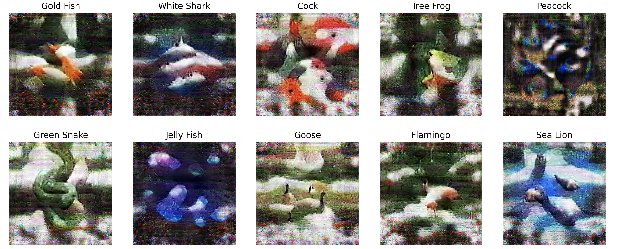
Figure 1: Visualization of distilled images generated using GUARD with 1 ipc setting from ImageNet.

We provide a visualization of the distilled images generated by GUARD in Fig. 1, utilizing a distillation scale of 1 image per class among selected ImageNet classes. It can be seen that the images exhibit characteristics that resemble a blend of multiple objects within their assigned class, highlighting the method’s capacity to capture essential features.

The results of our experiment are detailed in Table 2. It can be observed that GUARD consistently outperforms both SRe²L and MTT in terms of robustness across various attacks.

Interestingly, we observe a notable increase in clean accuracy upon incorporating GUARD. While enhancing clean accuracy was not the primary goal of GUARD, this outcome aligns with its function as a regularizer, potentially aiding in model generalization. In the context of dataset distillation, where the goal is to distill essential features of the original dataset into a much smaller subset, improving the generalization is expected to have positive effects on the performance.

Table 2: Evaluation of different dataset distillation methods under adversarial attacks on ImageNette, TinyImageNet, and ImageNet. The best results among all methods are highlighted in bold, second best are underlined.

Dataset	IPC	Attack	Methods
			GUARD	SRe2L	MTT	TESLA
ImageNette	10	None (Clean)	57.93	42.42	58.43	36.84
		PGD100	23.87	4.76	39.85	28.10
		Square	44.07	22.77	34.79	24.61
		AutoAttack	19.69	4.99	33.72	24.48
		CW	41.47	22.11	34.57	24.61
		MIM	21.80	4.76	39.20	28.15
	50	None (Clean)	80.86	80.15	59.69	36.21
		PGD100	41.42	12.30	41.13	28.72
		Square	72.81	61.50	36.72	25.34
		AutoAttack	42.47	12.91	35.46	27.21
		CW	58.67	53.42	36.54	29.01
		MIM	43.23	12.43	41.69	30.12
	100	None (Clean)	83.39	85.83	64.33	45.04
		PGD100	57.50	31.65	44.89	33.98
		Square	77.68	19.18	40.41	29.27
		AutoAttack	64.84	17.93	39.46	28.99
		CW	69.35	68.20	40.66	29.32
		MIM	65.07	18.98	44.89	33.98
TinyImageNet	10	None (Clean)	37.00	33.18	8.14	14.06
		PGD100	6.39	1.08	4.08	8.40
		Square	19.53	15.85	2.48	6.31
		AutoAttack	4.91	0.79	2.44	6.16
		CW	8.40	3.24	2.50	6.26
		MIM	6.51	1.10	4.08	8.40
	50	None (Clean)	55.61	56.42	17.84	28.24
		PGD100	15.63	0.27	5.62	12.12
		Square	36.93	15.50	3.84	10.39
		AutoAttack	13.84	0.16	3.52	10.01
		CW	20.46	12.12	3.66	10.13
		MIM	16.09	0.29	5.64	12.12
	100	None (Clean)	60.13	59.30	29.16	30.48
		PGD100	13.79	0.25	8.63	14.45
		Square	37.06	17.74	7.29	12.02
		AutoAttack	12.76	0.19	6.75	11.57
		CW	20.05	14.02	6.93	11.57
		MIM	14.35	0.24	8.63	14.45
ImageNet-1K	10	None (Clean)	27.25	21.30	-	-
		PGD100	5.25	0.55	-	-
		Square	17.88	18.02	-	-
		AutoAttack	3.33	0.34	-	-
		CW	7.68	3.21	-	-
		MIM	5.23	0.51	-	-
	50	None (Clean)	39.89	46.80	-	-
		PGD100	9.77	0.59	-	-
		Square	28.39	32.40	-	-
		AutoAttack	7.03	0.47	-	-
		CW	14.14	6.31	-	-
		MIM	9.84	0.64	-	-

5.4 Ablation

In Section 4.2, Eq. 7 showed that the adversarial loss is upper-bounded by the normal loss, the gradient magnitude, and the curvature term. GUARD regularizes the curvature term while disregarding the gradient magnitude, which could theoretically reduce the upper bound of the loss as well. Here, we investigate the effect of regularizing gradient instead of curvature and present the results in Table 3. The results indicate that GUARD outperforms the gradient regularization alternatives, regardless of the regularization parameter.

Table 3: Accuracy on ImageNette of original SRe²L, GUARD, and gradient regularization on SRe²L with regularization parameters ($\lambda_{g}=10^{-4},10^{-3},10^{-2},0.1,1$). The best results among all methods are highlighted in bold.

IPC	Attack	Methods
		SRe2L	GUARD	$\lambda_{g}=10^{-4}$	$\lambda_{g}=10^{-3}$	$\lambda_{g}=10^{-2}$	$\lambda_{g}=0.1$	$\lambda_{g}=1$
1	None (Clean)	27.97	37.49	13.72	16.15	16.41	17.58	18.75
	PGD100	12.05	16.22	6.39	9.32	10.27	10.39	13.27
	Square	18.62	26.74	9.71	11.69	13.68	12.94	15.97
	AutoAttack	12.12	15.81	6.32	9.35	10.17	10.42	13.25
	CW	20.38	29.14	7.62	11.06	11.64	11.31	14.47
	MIM	12.05	16.32	6.39	9.25	10.39	10.39	13.27
10	None (Clean)	42.42	57.93	44.82	41.81	42.80	43.34	40.31
	PGD100	4.76	23.87	15.39	14.47	15.41	13.68	16.92
	Square	22.77	44.07	34.06	31.80	34.73	31.85	31.03
	AutoAttack	4.99	19.69	15.62	14.52	15.64	13.78	16.87
	CW	22.11	41.47	21.58	20.64	21.17	18.85	21.53
	MIM	4.76	21.80	15.41	14.60	15.34	13.66	17.41
50	None (Clean)	80.15	80.86	76.46	74.06	73.12	74.52	-
	PGD100	12.30	41.42	35.54	35.36	33.48	29.17	-
	Square	61.50	72.81	67.08	63.24	63.97	65.53	-
	AutoAttack	12.91	42.47	35.59	35.54	33.52	29.32	-
	CW	53.42	58.67	46.06	45.43	44.05	41.02	-
	MIM	12.43	43.23	35.61	35.39	33.66	29.07	-

6 Discussion

6.1 Robustness Guarantee

Due to the nature of dataset distillation, it is impossible to optimize the robustness of the final model with respect to the real dataset. Therefore, most approaches in this direction, including ours, have to optimize the adversarial loss of the model with respect to the distilled dataset. Unfortunately, there is always a distribution shift between the real and distilled datasets, which raises uncertainties about whether robustness on the distilled dataset will be effectively transferred when evaluated against the real dataset.

Nevertheless, our theoretical framework offers assurances regarding this concern. A comparison between Eq. 6 with Eq. 7 reveals that the bounds of adversarial loss for real data and distilled data differ only by $L\sigma$. For a well-distilled dataset, $\sigma$ should be relatively small. We have thus demonstrated that the disparity between minimizing adversarial loss on the distilled dataset and on the real dataset is confined to this constant. This conclusion of our theory allows future robust dataset distillation methods to exclusively enhance robustness with respect to the distilled dataset, without worrying if the robustness can transfer well to the real dataset.

6.2 Computational Overhead

The structure of robust dataset distillation, as outlined in Eq. 4, inherently presents a tri-level optimization challenge. Typically, addressing such a problem could entail employing complex tri-level optimization algorithms, resulting in significant computational demands. One example of this is the integration of adversarial training within the distillation framework, which necessitates an additional optimization loop for generating adversarial examples within each iteration.

However, GUARD’s approach, as detailed in Eq. 11, introduces an efficient alternative. GUARD’s regularization loss only requires an extra forward pass to compute the loss $\ell(\mathbf{x}+h\mathbf{z})$ within each iteration. Therefore, integrating GUARD’s regularizer into an existing method does not significantly increase the overall computational complexity, ensuring that the computational overhead remains minimal. This efficiency is particularly notable given the computationally intensive nature of tri-level optimization in robust dataset distillation. In Table 4, we present a comparison of the time per iteration required for a tri-level optimization algorithm, such as the one used for embedded adversarial training described in Section 3.2, against the time required for GUARD. The findings show that GUARD is much more computationally efficient and has a lower memory usage as well.

Table 4: Computation overhead of GUARD compared with embedded adversarial training. Experiments are performed on one NVIDIA A100 80GB PCIe GPU with batch size 32. We measure 5 times per iteration training time and report the average and standard deviation. Adv Training follows Section 3.2.

Method	Time (s) / Iter	Peak Mem
GUARD	0.007 $\pm$ 2.661$e^{-4}$	3851MiB
Adv Training	2.198 $\pm$ 6.735$e^{-4}$	4211MiB

6.3 Transferability

Our investigation focuses on studying the effectiveness of the curvature regularizer within the SRe²L framework. Theoretically, this method can be extended to a broad spectrum of dataset distillation methods. GUARD’s application is feasible for any distillation approach that utilizes a model trained on the original dataset as a comparison target during the distillation phase — a strategy commonly seen across many dataset distillation techniques as noted in Section 2. This criterion is met by the majority of dataset distillation paradigms, with the exception of those following the distribution matching approach, which may not consistently employ a comparison model (Sachdeva and McAuley, 2023). This observation suggests GUARD’s potential compatibility with a wide array of dataset distillation strategies.

To demonstrate this, we explored two additional implementation of GUARD using DC (Zhao et al., 2021) and CDA (Yin and Shen, 2023) as baseline distillation methods. DC represents an earlier, simpler approach that leverages gradient matching for distillation purposes, whereas CDA is a more recent distillation technique, specifically designed for very large datasets. As shown in Table 5, GUARD consistently improves both clean accuracy and robustness across various dataset distillation methods.

Table 5: Direct comparison of the original DC, SRe²L, and CDA methods with the addition of GUARD regularizer on CIFAR10. The best results among each pair of compared methods are highlighted in bold.

IPC	Attack	Methods
		DC	GUARD(DC)	SRe2L	GUARD(SRe2L)	CDA	GUARD(CDA)
1	None (Clean)	29.96	30.95	17.13	22.88	14.98	23.18
	PGD100	24.59	46.88	13.56	19.21	12.69	18.70
	Square	24.72	48.56	13.75	19.55	12.84	19.17
	AutoAttack	24.33	14.99	13.43	18.91	12.63	18.42
	CW	24.58	15.19	13.52	18.95	12.62	18.52
	MIM	24.62	15.27	13.57	19.22	12.69	18.71
10	None (Clean)	45.38	46.83	26.58	30.76	20.55	30.65
	PGD100	31.84	32.36	18.24	22.31	14.60	24.33
	Square	33.71	33.54	19.99	24.16	15.93	25.66
	AutoAttack	31.05	31.84	18.11	21.58	14.47	24.04
	CW	31.95	32.35	18.73	21.98	14.83	24.51
	MIM	31.89	32.37	18.25	22.35	14.62	24.34
50	None (Clean)	-	-	43.96	44.05	36.32	43.05
	PGD100	-	-	24.74	33.12	21.58	33.02
	Square	-	-	29.68	35.22	25.76	35.19
	AutoAttack	-	-	24.45	32.24	21.46	31.96
	CW	-	-	26.09	32.67	22.54	32.56
	MIM	-	-	24.81	33.12	21.61	33.03

7 Conclusion

Our work focuses on a novel perspective on dataset distillation by emphasizing its robustness characteristics. Upon reaching the theoretical conclusion that the adversarial loss of distilled datasets is bounded by the curvature, we proposed GUARD, a method that can be integrated into many dataset distillation methods to provide robustness against diverse types of attacks and potentially improve clean accuracy. Our theory also provided the insight that the optimization of robustness with respect to distilled and real datasets is differentiated only by a constant term. This conclusion opens up various potentials for subsequent research in the field. We hope that our work contributes to the development of dataset distillation techniques that are not only efficient but also robust, and will inspire and support further research and development in this area.

Supplementary Material

Appendix A Proof of Proposition 1

The adversarial loss of an arbitrary input sample $\mathbf{x}$ can be upper-bounded as below:

$$\begin{split}\tilde{\ell}_{\rho}^{adv}(\mathbf{x})&=\max_{\|\mathbf{v}\|\leq\rho}\tilde{\ell}(\mathbf{x+v})=\max_{\|\mathbf{v}\|\leq\rho}\ell(\mathbf{x})+{\nabla\ell(\mathbf{x})}^{\top}\mathbf{v}+\frac{1}{2}\mathbf{v^{\top}Hv}\\ &\leq\max_{\|\mathbf{v}\|\leq\rho}\ell(\mathbf{x})+\|{\nabla\ell(\mathbf{x})}\|\|\mathbf{v}\|+\frac{1}{2}\lambda_{1}(\mathbf{x}){\|\mathbf{v}\|}^{2}\\ &=\ell(\mathbf{x})+\|{\nabla\ell(\mathbf{x})}\|\rho+\frac{1}{2}\lambda_{1}(\mathbf{x})\rho^{2},\end{split}$$ (12)

where $\lambda$ is the largest eigenvalue of the Hessian $\mathbf{H(\ell(x))}$.
Taking expectation over the distribution of real data with class label $c$, denoted as $D_{c}$,

$$\mathop{\mathbb{E}}_{\mathbf{x}\sim D_{c}}\tilde{\ell}_{\rho}^{adv}(\mathbf{x})\leq\mathop{\mathbb{E}}_{\mathbf{x}\sim D_{c}}\ell(\mathbf{x})+\rho\mathop{\mathbb{E}}_{\mathbf{x}\sim D_{c}}\|{\nabla\ell(\mathbf{x})}\|+\frac{1}{2}\rho^{2}\mathop{\mathbb{E}}_{\mathbf{x}\sim D_{c}}\lambda_{1}(\mathbf{x}).$$ (13)

With the assumption that $\tilde{\ell}(\mathbf{x})$ is convex, we know that $\tilde{\ell}_{\rho}^{adv}(\mathbf{x})$ is also convex, because $\forall\lambda\in[0,1],$

$$\begin{split}&\tilde{\ell}_{\rho}^{adv}(\lambda\mathbf{x}_{1}+(1-\lambda)\mathbf{x}_{2})\\ &=\max_{\|\mathbf{v}\|\leq\rho}\tilde{\ell}(\lambda\mathbf{x}_{1}+(1-\lambda)\mathbf{x}_{2}+\mathbf{v})\\ &=\max_{\|\mathbf{v}\|\leq\rho}\tilde{\ell}(\lambda(\mathbf{x}_{1}+\mathbf{v})+(1-\lambda)(\mathbf{x}_{2}+\mathbf{v}))\\ &\leq\max_{\|\mathbf{v}\|\leq\rho}\lambda\tilde{\ell}(\mathbf{x}_{1}+\mathbf{v})+(1-\lambda)\tilde{\ell}(\mathbf{x}_{2}+\mathbf{v})\\ &\leq\lambda\max_{\|\mathbf{v}\|\leq\rho}\tilde{\ell}(\mathbf{x}_{1}+\mathbf{v})+(1-\lambda)\max_{\|\mathbf{v}\|\leq\rho}\tilde{\ell}(\mathbf{x}_{2}+\mathbf{v})\\ &=\lambda\tilde{\ell}_{\rho}^{adv}(\mathbf{x}_{1})+(1-\lambda)\tilde{\ell}_{\rho}^{adv}(\mathbf{x}_{2}).\end{split}$$ (14)

Therefore, by Jensen’s Inequality,

$$\tilde{\ell}_{\rho}^{adv}(\mathop{\mathbb{E}}_{\mathbf{x}\sim D_{c}}\mathbf{x})\leq\mathop{\mathbb{E}}_{\mathbf{x}\sim D_{c}}\tilde{\ell}_{\rho}^{adv}(\mathbf{x}).$$ (15)

Let $\mathbf{x}^{\prime}$ be a datum distilled from the training data with class label $c$. It should be close in distribution to that of the real data. Hence, we can assume the maximum mean discrepancy (MMD) between the distilled data and real data is bounded as $\|h(\mathbf{x}^{\prime})-\mathbb{E}_{\mathbf{x}\sim D_{c}}h(\mathbf{x})\|\leq\sigma$, where $h(\cdot)$ is a feature extractor. If $h(\cdot)$ is invertible, then $\mathcal{L}_{\rho}^{adv}(\cdot)=\tilde{\ell}_{\rho}^{adv}(h^{-1}(\cdot))$ is a function defined on the feature space. We assume that $\mathcal{L}_{\rho}^{adv}(\cdot)$ is $L$-Lipschitz, it follows that

$$\mathcal{L}_{\rho}^{adv}(h(\mathbf{x}^{\prime}))\leq\mathcal{L}_{\rho}^{adv}(\mathop{\mathbb{E}}_{\mathbf{x}\sim D_{c}}h(\mathbf{x}))+L\sigma.$$ (16)

If we add the assumption that $h(\cdot)$ is linear, $\mathop{\mathbb{E}}_{\mathbf{x}\sim D_{c}}h(\mathbf{x})=h(\mathop{\mathbb{E}}_{\mathbf{x}\sim D_{c}}\mathbf{x})$, then

$$\tilde{\ell}_{\rho}^{adv}(\mathbf{x}^{\prime})\leq\tilde{\ell}_{\rho}^{adv}(\mathop{\mathbb{E}}_{\mathbf{x}\sim D_{c}}\mathbf{x})+L\sigma.$$ (17)

Combining  Eq. 13, Eq. 15, Eq. 17, we get

$$\tilde{\ell}_{\rho}^{adv}(\mathbf{x}^{\prime})\leq\mathop{\mathbb{E}}_{\mathbf{x}\sim D_{c}}\ell(\mathbf{x})+\rho\mathop{\mathbb{E}}_{\mathbf{x}\sim D_{c}}\|\nabla\ell(\mathbf{x})\|+\frac{1}{2}\rho^{2}\mathop{\mathbb{E}}_{\mathbf{x}\sim D_{c}}\lambda_{1}(\mathbf{x})+L\sigma.$$ (18)

Discussion

The inequality in line (2) is an equality if and only if the direction of the gradient is the same as the direction of $\lambda_{1}$. Previous work has empirically shown that the two directions have a large cosine similarity in the input space of neural networks. Our assumption about the Lipschitz continuity of $\mathcal{L}_{\rho}^{adv}(\cdot)$ is reasonable, as recent work has shown improved estimation of the Lipschitz constant of neural networks in a wide range of settings (Khromov and Singh, 2023). Although our assumptions about the convexity of $\tilde{\ell}(\mathbf{x})$ and the linearity of $h(\cdot)$ is relatively strong, it still reflects important aspects of reality, as our experiment in Table 2 has shown that reducing the curvature term in r.h.s of  Eq. 18 effectively improves the robustness of models trained on distilled data. Moreover, in Fig. 2 we plot the distribution of eigenvalues of the real data samples on the loss landscape of a model trained on standard distilled data and a model trained on robust distilled data from our GUARD method, respectively. GUARD corresponds to a flatter curve of eigenvalue distribution, indicating that the loss landscape becomes more linear after our regularization.

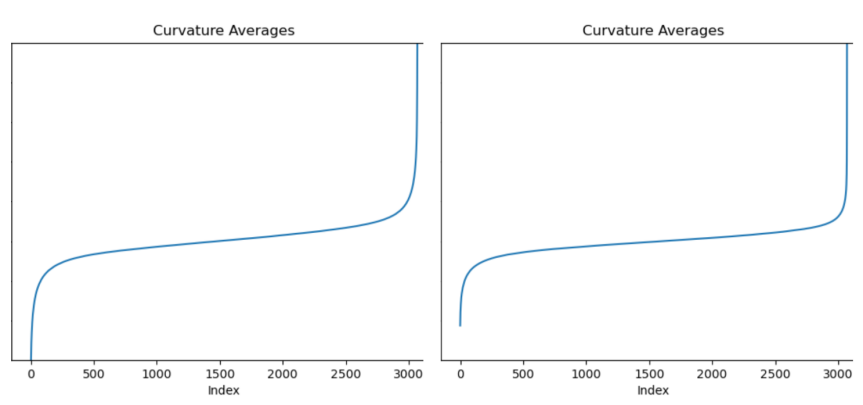
Figure 2: A comparison between the curvature profiles of a baseline dataset distillation method (left) and GUARD (right) in the form of sorted eigenvalues of the hessian

Appendix B Effect on GUARD on Images

In this section, we provide a detailed comparison between synthetic images produced by GUARD and those generated by other methods. In Fig. 3, we showcase distilled images from GUARD (utilizing SRe²L as a baseline) alongside images from SRe²L.

Our comparative analysis reveals that the images generated by the GUARD method appear to have more distinct object outlines when compared with those from the baseline SRe²L method. This improved definition of objects may facilitate better generalization in subsequent model training, which could offer an explanation for the observed increases in clean accuracy.

Additionally, our synthetic images exhibit a level of high-frequency noise, which bears similarity to the disruptions introduced by adversarial attacks. While visually subtle, this attribute might play a role in enhancing the resilience of models against adversarial inputs, as training on these images could prepare the models to handle unexpected perturbations more effectively. This suggests that the GUARD method could represent a significant advancement in the creation of synthetic datasets that promote not only visual fidelity but also improved robustness in practical machine learning applications.

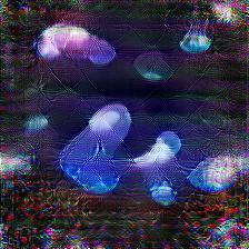
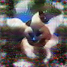
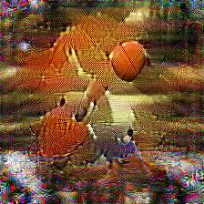
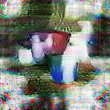
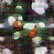
GUARD

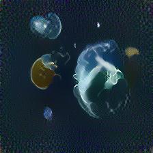
Jellyfish

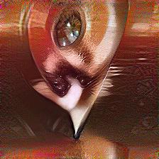
Siamese cat

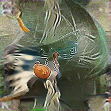
Basketball

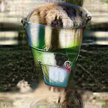
Bucket

Cello

SRe²L

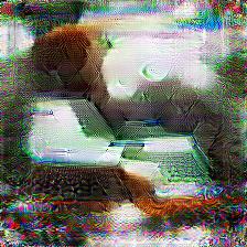
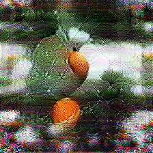
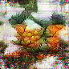
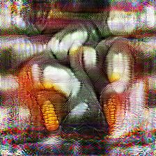
GUARD

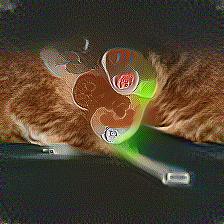
Laptop

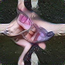
Sandal

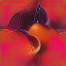
Orange

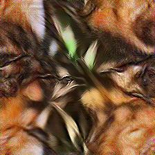
Pineapple

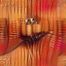
Corn

SRe²L

Figure 3: Comparative visualization of distilled images from GUARD and SRe²L with 1 ipc Setting on ImageNet.

Appendix C GUARD and Optimization-based Distillation Methods

In Section 4.4, we explained how GUARD can be easily intergrated into SRe²L by incorporating the regularizer into the model’s training loss during the squeeze (pre-training) step. We later demonstrated that GUARD could also be integrated into other distillation methods, such as DC (Zhao et al., 2021). However, unlike SRe²L, DC lacks a pre-training phase; instead, the model’s training and distillation occur simultaneously, making the integration less straightforward.

Therefore, we present the GUARD algorithm using DC as the baseline method in Algorithm 1. For each outer iteration $k$, we sample a new initial weight from some random distribution of weights to ensure the synthetic dataset can generalize well to a range of weight initializations. After, we iteratively sample a minibatch pair from the real dataset and the synthetic dataset and compute the loss over them on a neural network with the weights $\boldsymbol{\theta}_{t}$. We compute the regularized loss on real data through Eq. 11. Finally, we compute the gradient of the losses w.r.t. $\boldsymbol{\theta}$, and update the synthetic dataset through stochastic gradient descent on the distance between the gradients. At the end of each inner iteration $t$, we update the weights $\boldsymbol{\theta}_{t+1}$ using the updated synthetic dataset.

Input: $\mathcal{T}$: Training set; $\mathcal{S}$: initial synthetic dataset with $C$ classes; $p(\theta_{0})$: initial weights distribution; $\phi_{\theta}$: neural network; $K$: number of outer-loop steps; $T$: number of inner-loop steps; $\varsigma_{\theta}$: number of steps for updating weights; $\varsigma_{S}$: number of steps for updating synthetic samples; $\eta_{\theta}$: learning rate for updating weights; $\eta_{S}$: learning rate for updating synthetic samples; $D$: gradient distance function; $h$: discretization step; $\lambda$: strength of regularization

for each outer training step $k=1$ to $K$ do

       Sample initial weight $\theta_{0}\sim p(\theta_{0})$ ;

       for each inner training step $t=1$ to $T$ do

             for each class $c=1$ to $C$ do

                   Sample $\omega\sim\Omega$ and a minibatch pair $B^{\mathcal{T}}_{c}\sim\mathcal{T}$ and $B^{\mathcal{S}}_{c}\sim\mathcal{S}$;

                   Compute loss on synthetic data $\mathcal{L}^{\mathcal{S}}_{c}=\frac{1}{|B^{\mathcal{S}}_{c}|}\sum_{(\textbf{s},\textbf{y})\in B^{\mathcal{S}}_{c}}\ell(\phi_{\theta_{t}}(\textbf{s}),\textbf{y})$ ;

                   Compute loss on real data $\mathcal{L}^{\mathcal{T}}_{c}=\frac{1}{|B^{\mathcal{T}}_{c}|}\sum_{(\textbf{x},\textbf{y})\in B^{\mathcal{T}}_{c}}\ell(\phi_{\theta_{t}}(\textbf{x}),\textbf{y})$;

                   Compute $z=\frac{\nabla\ell(\phi_{\theta_{t}}(\textbf{s}),\textbf{y})}{\|\nabla\ell(\phi_{\theta_{t}}(\textbf{s},\textbf{y}))\|}$;

                   Compute loss on perturbed real data $\mathcal{L}^{\mathcal{T}_{z}}_{c}=\frac{1}{|B^{\mathcal{T}}_{c}|}\sum_{(\textbf{x},\textbf{y})\in B^{\mathcal{T}}_{c}}\ell(\phi_{\theta_{t}}(\textbf{x}+hz),\textbf{y})$;

                   Compute regularizer $\mathcal{R}=\nabla_{\theta}\mathcal{L}^{\mathcal{T}_{z}}_{c}(\theta_{t})-\nabla_{\theta}\mathcal{L}^{\mathcal{T}}_{c}(\theta_{t})$;

                   Compute regularized loss on real data $\mathcal{L}^{\mathcal{T}_{\mathcal{R}}}_{c}=\mathcal{L}^{\mathcal{T}}_{c}+\lambda\mathcal{R}$;

                   Update $\mathcal{S}_{c}\leftarrow\texttt{sgd}_{\mathcal{S}}(D(\nabla_{\theta}\mathcal{L}^{\mathcal{S}}_{c}(\theta_{t}),\nabla_{\theta}\mathcal{L}^{\mathcal{T}_{\mathcal{R}}}_{c}(\theta_{t})),\varsigma_{\mathcal{S}},\eta_{\mathcal{S}})$;

                  

             end for

            Update $\theta_{t+1}\leftarrow\texttt{sgd}_{\theta}(\mathcal{L}(\theta_{t},\mathcal{S}),\varsigma_{\theta},\eta_{\theta})$ ;

            

       end for

      

end for

Output: robust condensed dataset $\mathcal{S}$

Algorithm 1 DC-based GUARD

References

- Andriushchenko et al. (2020) M. Andriushchenko, F. Croce, N. Flammarion1, and M. Hein. Square attack: a query-efficient black-box adversarial attack via random search. In Proceedings of the European Conference on Computer Vision, 2020.
- Athalye et al. (2018) A. Athalye, N. Carlini, and D. Wagner. Obfuscated gradients give a false sense of security: Circumventing defenses to adversarial examples. arXiv preprint arXiv:1802.00420, 2018.
- Buzaglo et al. (2023) G. Buzaglo, N. Haim, G. Yehudai, G. Vardi, Y. Oz, Y. Nikankin, and M. Irani. Deconstructing data reconstruction: Multiclass, weight decay and general losses. arXiv preprint arXiv:2307.01827, 2023.
- Carlini and Wagner (2017) N. Carlini and D. Wagner. Towards evaluating the robustness of neural networks. In IEEE Symposium on Security and Privacy, pages 39–57, 2017.
- Cazenavette et al. (2022) G. Cazenavette, K. He, A. Torralba, A. A. Efros, and J.-Y. Zhu. Dataset distillation by matching training trajectories. In IEEE Conference on Computer Vision and Pattern Recognition, 2022.
- Chen et al. (2017) P.-Y. Chen, H. Zhang, Y. Sharma, J. Yi, and C.-J. Hsieh. Zoo: Zeroth order optimization based black-box attacks to deep neural networks without training substitute models. In Proceedings of the 10th ACM Workshop on Artificial Intelligence and Security, pages 15–26. ACM, 2017.
- Chen et al. (2023) Z. Chen, J. Geng, D. Zhu, H. Woisetschlaeger, Q. Li, S. Schimmler, R. Mayer, and C. Rong. A comprehensive study on dataset distillation: Performance, privacy, robustness and fairness. arXiv preprint arXiv:2305.03355, 2023.
- Cisse et al. (2017a) M. Cisse, Y. Adi, N. Neverova, and J. Keshet. Houdini: Fooling deep structured prediction models. arXiv preprint arXiv:1707.05373, 2017a.
- Cisse et al. (2017b) M. Cisse, P. Bojanowski, E. Grave, Y. Dauphin, and N. Usunier. Parseval networks: Improving robustness to adversarial examples. In Proceedings of the 34th International Conference on Machine Learning, pages 854–863, 2017b.
- Cohen et al. (2019) J. Cohen, E. Rosenfield, and Z. Kolter. Certified adversarial robustness via randomized smoothing. In International Conference on Machine Learning, 2019.
- Croce and Hein (2020) F. Croce and M. Hein. Reliable evaluation of adversarial robustness with an ensemble of diverse parameter-free attacks. In International Conference on Machine Learning, 2020.
- Cui et al. (2023) J. Cui, R. Wang, S. Si, and C.-J. Hsieh. Scaling up dataset distillation to imagenet-1k with constant memory. In International Conference on Machine Learning, 2023.
- Deng et al. (2009) J. Deng, W. Dong, R. Socher, L.-J. Li, K. Li, and L. Fei-Fei. Imagenet: A large-scale hierarchical image database. In 2009 IEEE conference on computer vision and pattern recognition, pages 248–255. Ieee, 2009.
- Dong et al. (2017) Y. Dong, T. Pang, H. Su, J. Zhu, X. Hu, and J. Li. Boosting adversarial attacks with momentum. In Proceedings of the IEEE Conference on Computer Vision and Pattern Recognition, 2017.
- Fawzi et al. (2018) A. Fawzi, S.-M. Moosavi-Dezfooli, P. Frossard, and S. Soatto. Empirical study of the topology and geometry of deep networks. In IEEE Conference on Computer Vision and Pattern Recognition, Jun 2018.
- Geng et al. (2023) J. Geng, Z. Chen, Y. Wang, H. Woisetschlaeger, Q. Li, S. Schimmler, R. Mayer, Z. Zhao, and C. Rong. A survey on dataset distillation: Approaches, applications, and future directions. arXiv preprint arXiv:2305.01975, 2023.
- Goodfellow et al. (2015) I. J. Goodfellow, J. Shlens, and C. Szegedy. Explaining and harnessing adversarial examples. In International Conference on Learning Representations, 2015.
- Gu and Rigazio (2014) S. Gu and L. Rigazio. Towards deep neural network architectures robust to adversarial examples, 2014.
- He et al. (2016) K. He, X. Zhang, S. Ren, and J. Sun. Deep residual learning for image recognition. In IEEE Conference on Computer Vision and Pattern Recognition, pages 770–778, 2016.
- Howard (2018) J. Howard. Imagenette, 2018. URL https://github.com/fastai/imagenette/.
- Jetley et al. (2018) S. Jetley, N. Lord, and P. Torr. With friends like these, who needs adversaries? In Advances in neural information processing systems, 2018.
- Khromov and Singh (2023) G. Khromov and S. P. Singh. Some intriguing aspects about lipschitz continuity of neural networks. arXiv preprint arXiv:2302.10886, 2023.
- Kurakin et al. (2017) A. Kurakin, I. Goodfellow, and S. Bengio. Adversarial examples in the physical world. International Conference on Learning Representations Workshops, 2017.
- Le and Yang (2015) Y. Le and X. Yang. Tiny imagenet visual recognition challenge. CS 231N, 7(7):3, 2015.
- Lee et al. (2022) S. Lee, S. Chun, S. Jung, S. Yun, and S. Yoon. Dataset condensation with contrastive signals. In International Conference on Machine Learning, 2022.
- Liu et al. (2023a) H. Liu, M. Chaudhary, and H. Wang. Towards trustworthy and aligned machine learning: A data-centric survey with causality perspectives, 2023a.
- Liu et al. (2023b) H. Liu, T. Xing, L. Li, V. Dalal, J. He, and H. Wang. Dataset distillation via the wasserstein metric. arXiv preprint arXiv:2311.18531, 2023b.
- Madry et al. (2017) A. Madry, A. Makelov, L. Schmidt, D. Tsipras, and A. Vladu. Towards deep learning models resistant to adversarial attacks. arXiv preprint arXiv:1706.06083, 2017.
- Madry et al. (2018) A. Madry, A. Makelov, L. Schmidt, D. Tsipras, and A. Vladu. Towards deep learning models resistant to adversarial attacks. In Proceedings of the International Conference on Learning Representations, 2018.
- Miyato et al. (2015) T. Miyato, S. ichi Maeda, M. Koyama, K. Nakae, and S. Ishii. Distributional smoothing with virtual adversarial training, 2015.
- Moosavi-Dezfooli et al. (2016) S.-M. Moosavi-Dezfooli, A. Fawzi, and P. Frossard. Deepfool: a simple and accurate method to fool deep neural networks. In Proceedings of the IEEE conference on computer vision and pattern recognition, pages 2574–2582, 2016.
- Moosavi-Dezfooli et al. (2019) S.-M. Moosavi-Dezfooli, A. Fawzi, J. Uesato, and P. Frossard. Robustness via curvature regularization, and vice versa. In Proceedings of the IEEE Conference on Computer Vision and Pattern Recognition, pages 9078–9086, 2019.
- Narodytska and Kasiviswanathan (2016) N. Narodytska and S. P. Kasiviswanathan. Simple black-box adversarial perturbations for deep networks, 2016.
- Nguyen et al. (2020) T. Nguyen, Z. Chen, and J. Lee. Dataset meta-learning from kernel ridge-regression. arXiv preprint arXiv:2011.00050, 2020.
- Nguyen et al. (2021) T. Nguyen, R. Novak, L. Xiao, and J. Lee. Dataset distillation with infinitely wide convolutional networks. Advances in Neural Information Processing Systems, 34:5186–5198, 2021.
- (36) N. Papernot, P. McDaniel, S. Jha, M. Fredrikson, Z. B. Celik, and A. Swami. The limitations of deep learning in adversarial settings. In 2016 IEEE European Symposium on Security and Privacy.
- Papernot et al. (2016a) N. Papernot, P. McDaniel, and I. Goodfellow. Transferability in machine learning: from phenomena to black-box attacks using adversarial samples. arXiv preprint arXiv:1605.07277, 2016a.
- Papernot et al. (2016b) N. Papernot, P. McDaniel, X. Wu, S. Jha, and A. Swami. Distillation as a defense to adversarial perturbations against deep neural networks. In 2016 IEEE Symposium on Security and Privacy (SP), pages 582–597. IEEE, 2016b.
- Ross and Doshi-Velez (2018) A. S. Ross and F. Doshi-Velez. Improving the adversarial robustness and interpretability of deep neural networks by regularizing their input gradients. In AAAI Conference on Artificial Intelligence, 2018.
- Sachdeva and McAuley (2023) N. Sachdeva and J. McAuley. Data distillation: a survey. arXiv preprint arXiv:2301.04272, 2023.
- Sucholutsky and Schonlau (2021) I. Sucholutsky and M. Schonlau. Soft-label dataset distillation and text dataset distillation. In 2021 International Joint Conference on Neural Networks (IJCNN), pages 1–8. IEEE, 2021.
- Tramèr et al. (2018) F. Tramèr, A. Kurakin, N. Papernot, I. Goodfellow, D. Boneh, and P. McDaniel. Ensemble adversarial training: attacks and defenses. In International Conference on Learning Representations, 2018.
- Wang et al. (2022) K. Wang, B. Zhao, X. Peng, Z. Zhu, S. Yang, S. Wang, G. Huang, H. Bilen, X. Wang, and Y. You. Cafe: Learning to condense dataset by aligning features. In IEEE Conference on Computer Vision and Pattern Recognition, 2022.
- Wang et al. (2018) T. Wang, J.-Y. Zhu, A. Torralba, and A. A. Efros. Dataset distillation. arXiv preprint arXiv:1811.10959, 2018.
- Wong et al. (2019) E. Wong, F. R. Schmidt, and J. Z. Kolter. Wasserstein adversarial examples via projected sinkhorn iterations. arXiv preprint arXiv:1902.07906, 2019.
- Yin and Shen (2023) Z. Yin and Z. Shen. Dataset distillation in large data era. arXiv preprint arXiv:2311.18838, 2023.
- Yin et al. (2023) Z. Yin, E. Xing, and Z. Shen. Squeeze, recover and relabel: Dataset condensation at imagenet scale from a new perspective. In Advances in Neural Information Processing Systems, 2023.
- Zhang et al. (2024) H. Zhang, S. Li, P. Wang, and S. Zeng, Dan Ge. M3D: Dataset condensation by minimizing maximum mean discrepancy. In Proceedings of the AAAI Conference on Artificial Intelligence (AAAI), 2024.
- Zhang et al. (2020) J. Zhang, X. Xu, B. Han, G. Niu, L. Cui, M. Sugiyama, and M. Kankanhalli. Attacks which do not kill training make adversarial learning stronger. In International Conference on Machine Learning, pages 11278–11287. PMLR, 2020.
- Zhao and Bilen (2021) B. Zhao and H. Bilen. Dataset condensation with differentiable siamese augmentation. In International Conference on Machine Learning, 2021.
- Zhao and Bilen (2023) B. Zhao and H. Bilen. Dataset condensation with distribution matching. In IEEE Winter Conference on Applications of Computer Vision, 2023.
- Zhao et al. (2021) B. Zhao, K. R. Mopuri, and H. Bilen. Dataset condensation with gradient matching. In International Conference on Learning Representations, 2021.
- Zhou et al. (2022) Y. Zhou, E. Nezhadarya, and J. Ba. Dataset distillation using neural feature regression. In Advances in Neural Information Processing Systems, 2022.