Multi-Fidelity Bayesian Optimization With Across-Task Transferable Max-Value
Entropy Search

Abstract

In many applications, ranging from logistics to engineering, a designer is faced with a sequence of optimization tasks for which the objectives are in the form of black-box functions that are costly to evaluate. For example, the designer may need to tune the hyperparameters of neural network models for different learning tasks over time. Rather than evaluating the objective function for each candidate solution, the designer may have access to approximations of the objective functions, for which higher-fidelity evaluations entail a larger cost. Existing multi-fidelity black-box optimization strategies select candidate solutions and fidelity levels with the goal of maximizing the information accrued about the optimal value or solution for the current task. Assuming that successive optimization tasks are related, this paper introduces a novel information-theoretic acquisition function that balances the need to acquire information about the current task with the goal of collecting information transferable to future tasks. The proposed method includes shared inter-task latent variables, which are transferred across tasks by implementing particle-based variational Bayesian updates. Experimental results across synthetic and real-world examples reveal that the proposed provident acquisition strategy that caters to future tasks can significantly improve the optimization efficiency as soon as a sufficient number of tasks is processed.

I Introduction

I-A Context and Scope

Numerous problems in logistics, science, and engineering can be formulated as black-box optimization tasks, in which the objective is costly to evaluate. Examples include hyperparameter optimization for machine learning [1], malware detection [2], antenna design [3], text to speech adaptation [4], material discovery [5], and resource allocation in wireless communication systems [6, 7, 8, 9]. To mitigate the problem of evaluating a costly objective function for each candidate solutions, the designer may have access to cheaper approximations of the optimization target. For example, the designer may be able to simulate a physical system using a digital twin that offers a controllable trade-off between cost and fidelity of the approximation [10, 11, 12, 13]. As shown in Fig. 1, higher-fidelity evaluations of the objective functions generally entail a larger cost, and the main challenge for the designer is to select a sequence of candidate solutions and fidelity levels that obtains the best solution within the available cost budget.

As a concrete example, consider the problem of optimizing the time spent by patients in a hospital’s emergency department [14]. The hospital may try different allocations of medical personnel by carrying out expensive real-world trials. Alternatively, one may adopt a simulator of patients’ hospitalization experiences, with different accuracy levels requiring a larger computing cost in terms of time and energy.

As also illustrated in Fig. 1, in many applications, the designer is faced with a sequence of black-box optimization tasks for which the objectives are distinct, but related. For instance, one may need to tune the hyperparameters of neural network models for different learning tasks over time; address the optimal allocation of personnel in a hospital in different periods of the year; or optimize resource allocation in a wireless system as the users’ demands change over time. As detailed in the next section, existing multi-fidelity black-box optimization strategies select candidate solutions and fidelity levels with the goal of maximizing the information accrued about the optimal value or solution for the current task.

This paper introduces a novel information-theoretic selection process for the next candidate solution and fidelity level that balances the need to acquire information about the current task with the goal of collecting information transferable to future tasks. The proposed method introduces shared latent variables across tasks. These variables are transferred across successive tasks by adopting a Bayesian formalism whereby the posterior distribution at the end of the current task is adopted as prior for the next task.

I-B Related Work

Bayesian optimization (BO) is a popular framework for black-box optimization problems. BO relies on a surrogate model, typically a Gaussian process (GP) [15], which encodes the current belief of the optimizer about the objective function, and an acquisition function that selects the next candidate solution based on the surrogate model [16, 17, 18, 19, 20]. BO has been extended to address multi-fidelity – also known as multi-task or multi-information source – settings [21, 22, 23]. Via multi-fidelity BO (MFBO), information collected at lower fidelity levels can be useful to accelerate the optimization process when viewed as a function of the overall cost budget for evaluating the objective function.

Prior works developed MFBO by building on standard BO acquisition functions, including expected improvement (EI) in [24], upper confidence bound (UCB) in [25], and knowledge gradient (KG) in [23, 26]. EI-based MFBO does not account for the level of uncertainty in the surrogate model. This issue is addressed by UCB-based approaches, which, however, require a carefully selected parameter to balance exploitation and exploration. Finally, although KG-based methods achieve efficient global optimization without hyperparameters in the acquisition function, empirical studies in [21] show that they incur a high computational overhead.

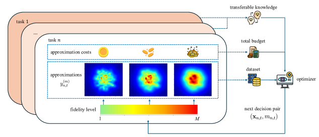
Figure 1: This paper studies a sequential multi-task optimization setting with multi-fidelity approximations of expensive-to-evaluate black-box objective functions. For any current task $n$, over time index $t=1,2,...,T_{n}$, the optimizer selects a pair of query point $\mathbf{x}_{n,t}$ and fidelity level $m_{n,t}$, requiring an approximation cost $\lambda^{(m)}$. As a result, the optimizer receives noisy feedback $y_{n,t}^{(m)}$ about target objective value $f_{n}(\mathbf{x}_{n,t})$. We wish to approach the global optimal solution $\mathbf{x}_{n}^{*}$ of objective $f_{n}(\mathbf{x})$ while abiding by a total simulation cost budget $\Lambda$.

In order to mitigate the limitations of the aforementioned standard acquisition functions, reference [22] introduced an information-theoretic acquisition function based on entropy search (ES) [27]. ES-based MFBO seeks for the next candidate solution by maximizing the information gain per unit cost. Accordingly, the ES-based acquisition functions aim to reduce the uncertainty about the global optimum, rather than to improve the current best solution as in EI- and KG-based methods, or to explore the most uncertain regions as in UCB-based approaches.

Reference [28] reduced the computation load of ES-based MFBO via max-value entropy search (MES) [19]; while the work [29] investigated parallel MFBO extensions. Theoretical and empirical comparisons between a light-weight MF-MES framework and other MFBO approaches are carried out in [21]. As shown recently in [30], the robustness of MF-MES can be guaranteed by introducing a novel mechanism of pseudo-observations when the feedback from lower fidelity levels is unreliable.

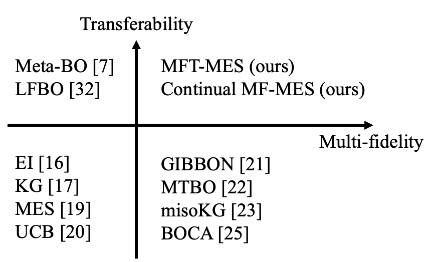
Figure 2: Comparison between selected prior works and the proposed MFT-MES method.

As illustrated in Fig. 2, the other axis of generalization of BO of interest for this work, namely transferability across tasks, has been much less investigated. This line of work relies on the assumption that sequentially arriving optimization tasks are statistically correlated, such that knowledge extracted from one task can be transferred to future tasks in the form of an optimized inductive bias encoded into the optimizer [31]. Existing studies fall into the categories of lifelong BO, which leverages previously trained deep neural networks to accelerate the optimizer training process exclusively on the new task [32]; and meta-learned BO, which learns a well-calibrated prior on the surrogate model given datasets collected from previous tasks [7, 33]. Using these methods, BO is seen to successfully transfer shared information across tasks, providing faster convergence on later tasks. However, these studies are limited to single-fidelity settings.

I-C Main Contributions

Assuming that successive optimization tasks are related, this paper introduces a novel information-theoretic acquisition function that balances the need to acquire information about the current task with the goal of collecting information transferable to future tasks. The proposed method, referred to as multi-fidelity transferable max-value entropy search (MFT-MES), includes shared inter-task latent variables, which are transferred across tasks by implementing particle-based variational Bayesian updates.

The main contributions are as follows.

• We introduce the MFT-MES, a novel black-box optimization scheme tailored for settings in which the designer is faced with a sequence of related optimization tasks. MFT-MES builds on MF-MES [21] by selecting candidate solutions and fidelity levels that maximize the information gain per unit cost. The information gain in MFT-MES accounts not only for the information about the optimal value of the current objective, as in MF-MES, but also for the information accrued on the inter-task shared latent parameters that can be transferred to future tasks. To this end, MFT-MES models the latent parameters as random quantities whose distributions are updated and transferred across tasks.

• As an efficient implementation of MFT-MES, we propose a particle-based variational inference (VI) update strategy for the latent shared parameters by leveraging Stein variational gradient descent (SVGD) [34].

• We present experimental results across synthetic tasks [35] and real-world examples [7, 36]. The results reveal that the provident acquisition strategy implemented by MFT-MES, which caters to future tasks, can significantly improve the optimization efficiency as soon as a sufficient number of tasks is processed.

I-D Organization

The rest of the paper is organized as follows. Sec. II formulates the sequential multi-task black-box optimization problem, and reviews the MF-GP surrogate model considered in the paper. Sec. III presents the baseline implementation of MF-MES, and illustrates the optimization over surrogate model parameters. The proposed MFT-MES method and the Bayesian update of the shared parameters are introduced in Sec. IV. Experimental results on synthetic optimization tasks and real-world applications are provided in Sec. V. Finally, Sec. VI concludes the paper.

II Problem Definition And Preliminaries

II-A Sequential Multi-Task Black-Box Optimization

We consider a setting in which optimization tasks, defined on a common input space $\mathcal{X}\subseteq\mathbbm{R}^{d}$, are addressed sequentially. Each $n$-th task, with $n=1,2,...$, consists of the optimization of a black-box expensive-to-evaluate objective function $f_{n}(\mathbf{x})$. Examples include the optimization of hyperparameters for machine learning models and experimental design [37, 38]. The objective functions $f_{n}(\mathbf{x})$ are assumed to be drawn according to a common parametric distribution $p(f(\mathbf{x})|\bm{\theta})$ in an independent identical distributed (i.i.d.) manner, i.e.,

$$f_{n}(\mathbf{x})\underset{\text{i.i.d.}}{\sim}p(f_{n}(\mathbf{x})|\bm{\theta})~{}\,\text{for}~{}\,n=1,2,...$$ (1)

Furthermore, the parameter vector $\bm{\theta}$ identifying the distribution $p(f(\mathbf{x})|\bm{\theta})$ is unknown, and it is assigned a prior distribution $p(\bm{\theta})$, i.e.,

$$\bm{\theta}\sim p(\bm{\theta}).$$ (2)

Note that, by (1) and (2), the objective function $f_{1}(\mathbf{x}),f_{2}(\mathbf{x}),...$ are not independent, since having information on any function $f_{n}(\mathbf{x})$ would reduce uncertainty on the parameters $\bm{\theta}$, thus also providing information about other function $f_{n^{\prime}}(\mathbf{x})$ with $n^{\prime}\neq n$.

For any current $n$-th task, the goal is to obtain an approximation of the optimal solution

$$\mathbf{x}_{n}^{*}=\arg\max_{\mathbf{x}\in\mathcal{X}}f_{n}(\mathbf{x})$$ (3)

with the minimal number of evaluations of function $f_{n}(\mathbf{x})$. To this end, this paper investigates the idea of selecting candidate solution $\mathbf{x}$ to query the current function $f_{n}(\mathbf{x})$ not only with the aim of approaching the solution in (3) for task $n$, but also to extract information about the common parameters $\bm{\theta}$ that may be useful for future optimization tasks $n^{\prime}>n$. This way, while convergence to a solution (3) may be slower for the current task $n$, future tasks may benefit from the acquired knowledge about parameters $\bm{\theta}$ to speed up convergence.

In order to account for the cost of accessing the objective function $f_{n}(\mathbf{x})$, we follow the multi-fidelity formulation, whereby evaluating function $f_{n}(\mathbf{x})$ at some querying point $\mathbf{x}$ with fidelity level $m$ entails a cost $\lambda^{(m)}>0$ [39, 40]. Different fidelity levels may correspond to training processes with varying number of iterations for hyperparameters optimization, or to simulations of a physical process with varying levels of accuracy for experimental desgin.

There are $M$ fidelity levels, listed from lower fidelity, $m=1$, to highest fidelity, $m=M$, which are collected in set $\mathcal{M}=\{1,2,...,M\}$. The function approximating objective $f_{n}(\mathbf{x})$ at the $m$-th fidelity level is denoted as $f_{n}^{(m)}(\mathbf{x})$. The costs are ordered from lowest fidelity to highest fidelity as

$$\lambda^{(1)}\leq\lambda^{(2)}\leq...\leq\lambda^{(M)},$$ (4)

and the highest-fidelity approximation coincides with the true objective function, i.e.,

$$f^{(M)}_{n}(\mathbf{x})=f_{n}(\mathbf{x}).$$ (5)

For each task $n$, the optimizer queries the objective function $f_{n}(\mathbf{x})$ during $T_{n}$ rounds, choosing at each round $t=1,...,T_{n}$, an input $\mathbf{x}_{n,t}$ and a fidelity level $m_{n,t}$. The number of rounds, $T_{n}$, is dictated by a cost budget, to be introduced below. The corresponding observation is given as

$$y^{(m)}_{n,t}=f_{n}^{(m)}(\mathbf{x}_{n,t})+\epsilon_{n,t},$$ (6)

where the observation noise variables $\epsilon_{n,t}\sim\mathcal{N}(0,\sigma^{2})$ are independent. Each pair $(\mathbf{x}_{n,t},m_{n,t})$ is chosen by the optimizer based on the past observations

$$\mathcal{D}_{n,t}=\Big{\{}(\mathbf{x}_{n,1},m_{n,1},y_{n,1}^{(m_{1})}),...,(\mathbf{x}_{n,t},m_{n,t},y_{n,t}^{(m_{t})})\Big{\}}$$ (7)

for the current task $n$, as well as based on the dataset

$$\mathcal{D}_{n-1}=\bigcup_{n^{\prime}=1}^{n-1}\mathcal{D}_{n^{\prime},T_{n^{\prime}}}$$ (8)

collected for all the previous tasks $n^{\prime}=1,...,n-1$. In practice, as we will see, data set $\mathcal{D}_{n-1}$ need not be explicitly stored. Rather, information in $\mathcal{D}_{n-1}$ that is useful for future tasks is summarized into a distribution over the shared parameter vector $\bm{\theta}$.

The number of rounds $T_{n}$ is determined by the cost constraint

$$\sum_{t=1}^{T_{n}}\lambda^{(m_{t})}\leq\Lambda$$ (9)

for each task $n$, where $\Lambda$ is a pre-determined total query cost budget for each optimization task. Accordingly, the number of rounds $T_{n}$ is the maximum integer such that constraint (9) is satisfied.

II-B Gaussian Process

The proposed approach builds on multi-fidelity GPs. To explain, we begin in this subsection with a brief review of conventional GP, which corresponds to the special case $M=1$ of a single fidelity level. With $M=1$, the optimizer maintains a single surrogate objective function for the true objective $f^{(1)}_{n}(\mathbf{x})=f_{n}(\mathbf{x})$ of each task $n$. In BO, this is done by assigning a zero-mean GP distribution $p(f_{n}|\bm{\theta})$ to function $f_{n}(\mathbf{x})$ that is characterized by a kernel function $k_{\bm{\theta}}(\mathbf{x},\mathbf{x}^{\prime})$, as denoted by

$$f_{n}\sim\mathcal{GP}(0,k_{\bm{\theta}}(\mathbf{x},\mathbf{x}^{\prime})).$$ (10)

The notation $k_{\bm{\theta}}(\mathbf{x},\mathbf{x}^{\prime})$ makes it clear that the kernel function, measuring the correlation of function values $f_{n}(\mathbf{x})$ and $f_{n}(\mathbf{x}^{\prime})$, depends on the common parameters $\bm{\theta}$ in (2).

By definition of GP, the collection of objective values $\mathbf{f}_{n,t}=[f_{n}(\mathbf{x}_{n,1}),...,f_{n}(\mathbf{x}_{n,t})]$ from any set of inputs $\mathbf{X}_{n,t}=[\mathbf{x}_{n,1},...,\mathbf{x}_{n,t}]$ follows a multivariate Gaussian distribution $\mathcal{N}(\mathbf{0},\mathbf{K}_{\bm{\theta}}(\mathbf{X}_{n,t}))$, with $t\times 1$ zero mean vector $\mathbf{0}$, and $t\times t$ covariance matrix $\mathbf{K}_{\bm{\theta}}(\mathbf{X}_{n,t})$ given by

$$\mathbf{K}_{\bm{\theta}_{n}}(\mathbf{X}_{n,t})=\begin{bmatrix}k_{\bm{\theta}_{n}}(\mathbf{x}_{n,1},\mathbf{x}_{n,1})&...&k_{\bm{\theta}_{n}}(\mathbf{x}_{n,1},\mathbf{x}_{n,t})\\ \vdots&\ddots&\vdots\\ k_{\bm{\theta}_{n}}(\mathbf{x}_{n,t},\mathbf{x}_{n,1})&...&k_{\bm{\theta}_{n}}(\mathbf{x}_{n,t},\mathbf{x}_{n,t})\end{bmatrix}.$$ (11)

A typical parametric kernel function is given by [41]

$$k_{\bm{\theta}}(\mathbf{x},\mathbf{x}^{\prime})=\exp{(-||\psi_{\bm{\theta}}(\mathbf{x})-\psi_{\bm{\theta}}(\mathbf{x}^{\prime})||_{2}^{2}}),$$ (12)

where $\psi_{\bm{\theta}}(\cdot)$ is a neural network with parameters $\bm{\theta}$.

Given any observation history $\mathcal{D}_{n,t}$ for task $n$ in (7), and given a parameter vector $\bm{\theta}$, the posterior distribution of objective value $f_{n}(\mathbf{x})$ at any input $\mathbf{x}$ is the Gaussian distribution [15]

$$p_{\bm{\theta}}(f_{n}(\mathbf{x})|\mathcal{D}_{n,t})=\mathcal{N}(\mu_{\bm{\theta}}(\mathbf{x}|\mathcal{D}_{n,t}),\sigma_{\bm{\theta}}^{2}(\mathbf{x}|\mathcal{D}_{n,t})),$$ (13)

where

$$\mu_{\bm{\theta}}(\mathbf{x}|\mathcal{D}_{n,t})=\mathbf{k}_{\bm{\theta}}(\mathbf{x})^{\sf T}(\tilde{\mathbf{K}}_{\bm{\theta}}(\mathbf{X}_{n,t}))^{-1}\mathbf{y}_{n,t},$$ (14a)

$$\text{and}\quad\sigma_{\bm{\theta}}^{2}(\mathbf{x}|\mathcal{D}_{n,t})=k_{\bm{\theta}}(\mathbf{x},\mathbf{x})-\mathbf{k}_{\bm{\theta}}(\mathbf{x})^{\sf T}(\tilde{\mathbf{K}}_{\bm{\theta}}(\mathbf{X}_{n,t}))^{-1}\mathbf{k}_{\bm{\theta}}(\mathbf{x}),$$ (14b)

with the $t\times t$ Gramian matrix $\tilde{\mathbf{K}}_{\bm{\theta}}(\mathbf{X}_{n,t})=\mathbf{K}_{\bm{\theta}}(\mathbf{X}_{n,t})+\sigma^{2}\mathbf{I}_{t}$; the $t\times 1$ cross-variance vector $\mathbf{k}_{\bm{\theta}}(\mathbf{x})=[k_{\bm{\theta}}(\mathbf{x},\mathbf{x}_{n,1}),\ldots,k_{\bm{\theta}}(\mathbf{x},\mathbf{x}_{n,t})]^{\sf T}$; and the $t\times 1$ observations vector $\mathbf{y}_{n,t}=[y_{n,1},...,y_{n,t}]^{\sf T}$.

II-C Multi-fidelity Gaussian Process

Multi-fidelity GP (MFGP) provides a surrogate model for the objective functions $(f_{n}^{(1)}(\mathbf{x}),...,f_{n}^{(M)}(\mathbf{x}))$ across all $M$ fidelity levels [42, 43, 44]. This is done by defining a kernel function of the form $k_{\bm{\theta}}\big{(}(\mathbf{x},m),(\mathbf{x}^{\prime},m^{\prime})\big{)}$ that captures the correlations between the function values $f_{n}^{(m)}(\mathbf{x})$ and $f_{n}^{(m^{\prime})}(\mathbf{x}^{\prime})$ for any two inputs $\mathbf{x}$ and $\mathbf{x}^{\prime}$, and for any two fidelity levels $m$ and $m^{\prime}$. Examples of such kernels include the co-kriging model in [44] and the intrinsic coregionalization model (ICM) kernel [42, 45], which is expressed as

$$k_{\bm{\theta}}\big{(}(\mathbf{x},m),(\mathbf{x}^{\prime},m^{\prime})\big{)}=k_{\bm{\theta}}(\mathbf{x},\mathbf{x}^{\prime})\cdot\kappa_{\bm{\theta}}(m,m^{\prime}),$$ (15)

where the input-space kernel $k_{\bm{\theta}}(\mathbf{x},\mathbf{x}^{\prime})$ is defined as in the previous subsection; while the fidelity space kernel $\kappa_{\bm{\theta}}(m,m^{\prime})$ is often instantiated as a radial basis function (RBF) kernel

$$\kappa(m,m^{\prime})=\exp(-\gamma||m-m^{\prime}||^{2}),$$ (16)

where the bandwidth parameter $\gamma$ is included in the hyperparameters $\bm{\theta}$. The MFGP prior for functions $f_{n}^{(1)}(\mathbf{x}),...,f_{n}^{(M)}(\mathbf{x})$ is denoted as

$$\Big{(}f_{n}^{(1)}(\mathbf{x}),...,f_{n}^{(M)}(\mathbf{x})\Big{)}\sim\mathcal{GP}(0,k_{\bm{\theta}}((\mathbf{x},m),(\mathbf{x}^{\prime},m^{\prime}))).$$ (17)

Let $\mathbf{y}_{n,t}=[y^{(m_{1})}_{n,1},...,y^{(m_{t})}_{n,t}]^{\sf T}$ denote the $t\times 1$ observations vector, and $\mathbf{m}_{n,t}=[m_{n,1},...,m_{n,t}]^{\sf T}$ be the $t\times 1$ vector of queried fidelity levels. Using the $t\times t$ kernel matrix $\mathbf{K}_{\bm{\theta}}(\mathbf{X}_{n,t},\mathbf{m}_{n,t})$ in which the $(i,j)$-th element $k_{\bm{\theta}}((\mathbf{x}_{n,i},m_{n,i}),(\mathbf{x}_{n,j},m_{n,j}))$ is defined as in (15), the MFGP posterior mean and variance at any input $\mathbf{x}$ with fidelity $m$ given the observation history $\mathcal{D}_{n,t}$ can be expressed as [29]

$$\mu^{(m)}_{\bm{\theta}}(\mathbf{x}|\mathcal{D}_{n,t})=\mathbf{k}_{\bm{\theta}}(\mathbf{x},m)^{\sf T}(\tilde{\mathbf{K}}_{\bm{\theta}}(\mathbf{X}_{n,t},\mathbf{m}_{n,t}))^{-1}\mathbf{y}_{n,t},$$ (18a)

$$[\sigma_{\bm{\theta}}^{(m)}(\mathbf{x}|\mathcal{D}_{n,t})]^{2}= k_{\bm{\theta}}((\mathbf{x},m),(\mathbf{x},m))$$

$$-\mathbf{k}_{\bm{\theta}}(\mathbf{x},m)^{\sf T}(\tilde{\mathbf{K}}_{\bm{\theta}}(\mathbf{X}_{n,t},\mathbf{m}_{n,t}))^{-1}\mathbf{k}_{\bm{\theta}}(\mathbf{x},m),$$ (18b)

where $\tilde{\mathbf{K}}_{\bm{\theta}}(\mathbf{X}_{n,t},\mathbf{m}_{n,t})=\mathbf{K}_{\bm{\theta}}(\mathbf{X}_{n,t},\mathbf{m}_{n,t})+\sigma^{2}\mathbf{I}_{t}$ is the $t\times t$ Gramian matrix.

Based on (18), an estimated value of the objective $f^{(m)}_{n}(\mathbf{x})$ can be obtained as the mean $\mu^{(m)}_{\bm{\theta}}(\mathbf{x}|\mathcal{D}_{n,t})$ in (18a), and the corresponding uncertainty of the estimate can be quantified by the variance $[\sigma_{\bm{\theta}}^{(m)}(\mathbf{x}|\mathcal{D}_{n,t})]^{2}$ in (18b).

III Single-Task Multi-fidelity Bayesian Optimization

In this section, we review a baseline implementation of MFBO based on MES [19, 21], which applies separately to each task $n$, without attempting to transfer knowledge across tasks.

III-A Multi-Fidelity Max-Value Entropy Search

For brevity of notation, we henceforth omit the dependence on the observation history $\mathcal{D}_{n,t}$ of the MFGP posterior mean $\mu^{(m)}_{\bm{\theta}}(\mathbf{x}|\mathcal{D}_{n,t})$ and variance $[\sigma_{\bm{\theta}}^{(m)}(\mathbf{x}|\mathcal{D}_{n,t})]^{2}$ in (18), writing $\mu^{(m)}_{\bm{\theta}}(\mathbf{x})$ and $[\sigma^{(m)}_{\bm{\theta}}(\mathbf{x})]^{2}$, respectively. Throughout this subsection, the parameter vector $\bm{\theta}$ is fixed, and the selection of $\bm{\theta}$ is discussed in the next subsection. In general multi-fidelity max-value entropy search (MF-MES) [21], at each time $t$, the next input $\mathbf{x}_{n,t+1}$ is selected, together with the fidelity level $m_{n,t+1}$, so as to maximize the ratio between the informativeness of the resulting observation $y_{n}^{(m)}$ in (6) and the cost $\lambda^{(m)}$.

Informativeness is measured by the mutual information between the optimal value $f_{n}(\mathbf{x}_{n}^{*})=f_{n}^{*}$ of the objective and the observation $y_{n}^{(m)}$ corresponding to input $\mathbf{x}_{n,t+1}$ at fidelity level $m$. Accordingly, the next pair $(\mathbf{x}_{n,t+1},m_{n,t+1})$ is obtained by maximizing the information gain per cost unit as

$$(\mathbf{x}_{n,t+1},m_{n,t+1})=\arg\max\limits_{\begin{subarray}{c}\mathbf{x}\in\mathcal{X}\\ m\in\mathcal{M}\end{subarray}}\frac{I(f_{n}^{*};y_{n}^{(m)}|\mathbf{x},\bm{\theta},\mathcal{D}_{n,t})}{\lambda^{(m)}}.$$ (19)

In (19), the mutual information is evaluated with respect to the joint distribution

$$p(f_{n}^{*},f_{n}^{(m)}(\mathbf{x}),y_{n}^{(m)}|\mathbf{x},\bm{\theta},\mathcal{D}_{n,t})$$

$$=p(f_{n}^{*},f_{n}^{(m)}(\mathbf{x})|\mathbf{x},\bm{\theta},\mathcal{D}_{n,t})p(y_{n}^{(m)}|f_{n}^{(m)}(\mathbf{x})),$$ (20)

where $p(f_{n}^{*},f_{n}^{(m)}(\mathbf{x})|\mathbf{x},\bm{\theta},\mathcal{D}_{n,t})$ follows the posterior GP in (18), and $p(y_{n}^{(m)}|f_{n}^{(m)}(\mathbf{x}))$ is defined by the observation model (6). Note that, to evaluate (19), the true, unobserved, function value $f_{n}^{(m)}(\mathbf{x})$ must be marginalized over.

Let us write as $H(\mathbf{y}|\mathbf{x})$ for the differential entropy of a variable $\mathbf{y}$ given a variable $\mathbf{x}$. By definition, the mutual information in (19) can be expressed as the difference of differential entropies [46]

$$I(f_{n}^{*};y_{n}^{(m)}|\mathbf{x},\bm{\theta},\mathcal{D}_{n,t})$$

$$=H(y_{n}^{(m)}|\mathbf{x},\bm{\theta},\mathcal{D}_{n,t})$$

$$\quad-\mathbbm{E}_{p(f_{n}^{*}|\mathbf{x},\bm{\theta},\mathcal{D}_{n,t})}[H(y_{n}^{(m)}|f_{n}^{*},\mathbf{x},\bm{\theta},\mathcal{D}_{n,t})]$$

$$=\log(\sqrt{2\pi e}\sigma_{\bm{\theta}}^{(m)}(\mathbf{x}))$$

$$\quad-\mathbbm{E}_{p(f_{n}^{*}|\mathbf{x},\bm{\theta},\mathcal{D}_{n,t})}[H(y_{n}^{(m)}|f_{n}^{(m)}(\mathbf{x})\leq f_{n}^{*},\mathbf{x},\bm{\theta},\mathcal{D}_{n,t})],$$ (21)

where the variance $[\sigma_{\bm{\theta}}^{(m)}(\mathbf{x})]^{2}$ is as in (18b), and (21) relies on the assumption that the $m$-th surrogate function $f_{n}^{(m)}(\mathbf{x})$ cannot attain a value larger than the maximum $f_{n}^{*}$ of the true objective function $f_{n}(\mathbf{x})$. Alternatively, one can remove this assumption by adopting a more complex approximation illustrated as in [29]. In MF-MES, the second term in (21) is approximated as [21]

$$H(y_{n}^{(m)}|f_{n}^{(m)}(\mathbf{x})\leq f_{n}^{*},\mathbf{x},\bm{\theta},\mathcal{D}_{n,t})$$

$$\approx\log\Bigg{(}\sqrt{2\pi e}\sigma_{\bm{\theta}}^{(m)}(\mathbf{x})\bigg{(}1-\frac{\phi(\gamma_{\bm{\theta}}^{(m)}(\mathbf{x},f_{n}^{*}))}{\Phi(\gamma_{\bm{\theta}}^{(m)}(\mathbf{x},f_{n}^{*}))}$$

$$\quad\bigg{[}\gamma_{\bm{\theta}}^{(m)}(\mathbf{x},f_{n}^{*})+\frac{\phi(\gamma_{\bm{\theta}}^{(m)}(\mathbf{x},f_{n}^{*}))}{\Phi(\gamma_{\bm{\theta}}^{(m)}(\mathbf{x},f_{n}^{*}))}\bigg{]}\bigg{)}\Bigg{)}$$

$$=H_{\bm{\theta}}^{\text{MF-MES}}(\mathbf{x},m,f^{*}_{n})$$ (22)

$$\text{with}\quad\gamma_{\bm{\theta}}^{(m)}(\mathbf{x},f_{n}^{*})=\frac{f_{n}^{*}-\mu_{\bm{\theta}}^{(m)}(\mathbf{x})}{\sigma_{\bm{\theta}}^{(m)}(\mathbf{x})},$$ (23)

where $\phi(\cdot)$ and $\Phi(\cdot)$ are the probability density function and cumulative density function of a standard Gaussian distribution, respectively. Intuitively, function $H_{\bm{\theta}}^{\text{MF-MES}}(\mathbf{x},m,f^{*}_{n})$ in (23) captures the uncertainty on the observation $y_{n}^{(m)}$ that would be produced by querying the objective at input $\mathbf{x}$ and fidelity level $m$ when the optimal value $f_{n}^{*}$ is known. This uncertainty should be subtracted, as per (21), from the overall uncertainty $H(y_{n}^{(m)}|\mathbf{x},\bm{\theta},\mathcal{D}_{n,t})$ in order to assess the extent to which the observation $y_{n}^{(m)}$ provides information about the optimal value $f_{n}^{*}$.

Using (22) in (21) and replacing the expectation in (21) with an empirical average, MF-MES selects the next query as

$$(\mathbf{x}_{n,t+1},m_{n,t+1})=\arg\max\limits_{\begin{subarray}{c}\mathbf{x}\in\mathcal{X}\\ m\in\mathcal{M}\end{subarray}}\alpha_{\bm{\theta}}^{\text{MF-MES}}(\mathbf{x},m),$$ (24)

where we have defined the MF-MES acquisition function

$$\alpha_{\bm{\theta}}^{\text{MF-MES}}(\mathbf{x},m)= \frac{1}{\lambda^{(m)}}\log(\sqrt{2\pi e}\sigma_{\bm{\theta}}^{(m)}(\mathbf{x}))$$

$$-\frac{1}{|\mathcal{F}|\lambda^{(m)}}\sum_{f_{n}^{*}\in\mathcal{F}}H_{\bm{\theta}}^{\text{MF-MES}}(\mathbf{x},m,f_{n}^{*}),$$ (25)

where the set $\mathcal{F}=\{f_{n,s}^{*}\}_{s=1}^{S}$ collects $S$ samples drawn from distribution $p_{\bm{\theta}}(f_{n}^{*}|\mathbf{x},\mathcal{D}_{n,t})$, which can be obtained via Gumbel sampling [19] and function $H_{\bm{\theta}}^{\text{MF-MES}}(\mathbf{x},m,f_{n}^{*})$ is defined in (22).

The overall procedure of MF-MES is summarized in Algorithm 1.

Input : Vector $\bm{\theta}$, simulation costs $\{\lambda^{(m)}\}_{m=1}^{M}$, query budget $\Lambda$

Output : Optimized solution $\mathbf{x}^{\text{opt}}$

1 Initialize iteration $t=0$, observation dataset $\mathcal{D}_{n,t}=\emptyset$, and $\Lambda^{0}=\Lambda$

2 while $\Lambda^{t}>0$ do

3       Sample max-value set $\mathcal{F}$ from distribution $p_{\bm{\theta}}(f_{n}^{*}|\mathbf{x},\mathcal{D}_{n,t})$

4       Obtain the next decision pair $(\mathbf{x}_{n,t+1},m_{n,t+1})$ via (24)

5       Observe $y_{n,t+1}^{(m)}$ in (6) and update observation history $\mathcal{D}_{n,t+1}=\mathcal{D}_{n,t}\cup(\mathbf{x}_{n,t+1},m_{n,t+1},y^{(m_{n,t+1})}_{n,t+1})$

6       Update the MFGP posterior as in (18)

7       Calculate remaining budget $\Lambda^{(t+1)}=\Lambda^{(t)}-\lambda^{(m_{n,t+1})}$

8       Set iteration $T_{n}=t$ and $t=t+1$

9 end while

10Return $\mathbf{x}^{\text{opt}}=\arg\max\limits_{t=1,..,T_{n}}f^{(M)}_{n}(\mathbf{x}_{n,t})$

Algorithm 1 Multi-Fidelity Max-Value Entropy Search (MF-MES) [21]

III-B Optimizing the Parameter Vector $\bm{\theta}$

In Sec. III-A, we have treated the parameter vector $\bm{\theta}$ as fixed. In practice, given the data set $\mathcal{D}_{n,t}$ collected up to round $t$ for the current task $n$, it is possible to update the parameter vector $\bm{\theta}$ to fit the available observations [15]. This is typically done by maximizing the marginal likelihood of parameters $\bm{\theta}$ given data $\mathcal{D}_{n,t}$.

Under the posterior distribution defined by (18a) and (18b), the negative marginal log-likelihood of the parameter vector $\bm{\theta}$ is given by

$$\ell(\bm{\theta}|\mathcal{D}_{n,t}) =-\log\big{(}p(\mathbf{y}_{n,t}|\bm{\theta})\big{)}$$

$$=-\frac{1}{2}\Bigg{(}t\log 2\pi-\log\Big{|}\tilde{\mathbf{K}}_{\bm{\theta}}(\mathbf{X}_{n,t},\mathbf{M}_{n,t})\Big{|}$$

$$\quad\,-\mathbf{y}_{n,t}^{\sf T}\Big{(}\tilde{\mathbf{K}}_{\bm{\theta}}(\mathbf{X}_{n,t},\mathbf{M}_{n,t})\Big{)}^{-1}\mathbf{y}_{n,t}\Bigg{)}.$$ (26)

where $p(\mathbf{y}_{n,t}|\bm{\theta})$ represents the probability density function of observation in (6). The negative marginal log-likelihood (26) can be interpreted as a loss function associated with parameters $\bm{\theta}$ based on the observations in data set $\mathcal{D}_{n,t}$. Accordingly, using the prior distribution (2), a maximum a posterior (MAP) solution for the parameter vector $\bm{\theta}$ is obtained by addressing the problem

$$\bm{\theta}_{n,t}^{\text{MAP}}=\arg\min\limits_{\bm{\theta}\in\bm{\Theta}}\{\ell(\bm{\theta}|\mathcal{D}_{n,t})-\log\big{(}p(\bm{\theta})\big{)}\},$$ (27)

where $p(\bm{\theta})$ is the prior distribution in (2), and the term $\log\big{(}p(\bm{\theta})\big{)}$ plays the role of a regularizer. To reduce computational complexity, the optimization problem (27) may be addressed periodically with respect to the round index $t$ [47, 6].

IV Sequential Multi-fidelity Bayesian Optimization With Transferable Max-Value Entropy Search

As reviewed in the previous section, MF-MES treats each task $n$ separately [29, 21]. However, since by (1) and (2), the successive objective functions $f_{1},...,f_{n}$ are generally correlated, knowledge extracted from one task can be transferred to future tasks through the common parameters $\bm{\theta}$ [48]. In this section, we introduce a novel information-theoretic acquisition function that generalizes the MF-MES acquisition function in (19) to account for the information acquired about parameters $\bm{\theta}$ for future tasks. The proposed approach, referred to as multi-fidelity transferable max-value entropy search (MFT-MES), hinges on a Bayesian formulation for the problem of sequentially estimating parameter vector $\bm{\theta}$ as more tasks are observed. In this section, we first describe the proposed acquisition function, and then describe an efficient implementation of the Bayesian estimation of parameter vector $\bm{\theta}$ based on Stein variational gradient descent (SVGD) [34].

IV-A Multi-Fidelity Transferable Max-Value Entropy Search

MFT-MES introduces a term in the MF-MES acquisition function (19) that promotes the selection of inputs $\mathbf{x}$ and fidelity levels $m$ that maximize the information brought by the corresponding observation $y_{n,t}^{(m)}$ about the parameters $\bm{\theta}$. The rationale behind this modification is that collecting information about the shared parameters $\bm{\theta}$ can potentially improve the optimization process for future tasks $n^{\prime}>n$.

Accordingly, MFT-MES adopts an acquisition function that measures the mutual information between the observation $y_{n}^{(m)}$ and, not only the optimal value $f_{n}^{*}$ for the current task $n$ in MF-MES, but also the common parameters $\bm{\theta}$. Note that, unlike MF-MES, this approach views the parameter vector $\bm{\theta}$ as a random quantity that is jointly distributed with the objective and with the observations. Normalizing by the cost $\lambda^{(m)}$ as in (19), MFT-MES selects the next query $(\mathbf{x}_{n,t+1},m_{n,t+1})$ with the aim of addressing the problem

$$(\mathbf{x}_{n,t+1},m_{n,t+1})=\arg\max\limits_{\begin{subarray}{c}\mathbf{x}\in\mathcal{X}\\ m\in\mathcal{M}\end{subarray}}\frac{I(f_{n}^{*},\bm{\theta};y_{n}^{(m)}|\mathbf{x},\mathcal{D}_{n-1},\mathcal{D}_{n,t})}{\lambda^{(m)}},$$ (28)

which is evaluated with respect to the joint distribution

$$p(f_{n}^{*},f_{n}^{(m)}(\mathbf{x}),\bm{\theta},y_{n}^{(m)}|\mathbf{x},\mathcal{D}_{n-1},\mathcal{D}_{n,t})$$

$$=p(\bm{\theta}|\mathcal{D}_{n-1},\mathcal{D}_{n,t})p(f_{n}^{*},f_{n}^{(m)}(\mathbf{x})|\mathbf{x},\bm{\theta},\mathcal{D}_{n,t})p(y_{n}^{(m)}|f_{n}^{(m)}(\mathbf{x})),$$ (29)

where the distribution $p(\bm{\theta}|\mathcal{D}_{n-1},\mathcal{D}_{n,t})$ is the posterior distribution on the shared model parameters $\bm{\theta}$. This distribution represents the transferable knowledge extracted from all the available observations at round $t$ for task $n$.

Using the chain rule for mutual information [46], the acquisition function (28) is expressed as

$$\alpha^{\text{MFT-MES}}(\mathbf{x},m)$$

$$=\frac{1}{\lambda^{(m)}}\Big{[}\mathbbm{E}_{p(\bm{\theta}|\mathcal{D}_{n-1},\mathcal{D}_{n,t})}\big{[}I(f_{n}^{*};y_{n}^{(m)}|\mathbf{x},\bm{\theta},\mathcal{D}_{n,t})\big{]}$$

$$\quad+I(\bm{\theta};y_{n}^{(m)}|\mathbf{x},\mathcal{D}_{n-1},\mathcal{D}_{n,t})\Big{]}.$$ (30)

In (30), the first term is the expected information gain on the global optimum $f_{n}^{*}$ that is also included in the MF-MES acquisition function in (19), while the second term in (30) quantifies transferable knowledge via the information gain about the shared parameters $\bm{\theta}$.

The second term in (30) can be written more explicitly as

$$I(\bm{\theta};y_{n}^{(m)}|\mathbf{x},\mathcal{D}_{n-1},\mathcal{D}_{n,t})$$

$$=H(y_{n}^{(m)}|\mathbf{x},\mathcal{D}_{n-1},\mathcal{D}_{n,t})$$

$$\quad-\mathbbm{E}_{p(\bm{\theta}|\mathcal{D}_{n-1},\mathcal{D}_{n,t})}\big{[}H(y^{(m)}_{n}|\mathbf{x},\bm{\theta},\mathcal{D}_{n,t})\big{]}$$

$$=H\bigg{(}\mathbb{E}_{p(\bm{\theta}|\mathcal{D}_{n-1},\mathcal{D}_{n,t})}\Big{[}p(y_{n}^{(m)}|\mathbf{x},\bm{\theta},\mathcal{D}_{n,t})\Big{]}\bigg{)}$$

$$\quad-\frac{1}{2}\mathbb{E}_{p(\bm{\theta}|\mathcal{D}_{n-1},\mathcal{D}_{n,t})}\Big{[}\log\Big{(}2\pi e\big{[}\sigma_{\bm{\theta}}^{(m)}(\mathbf{x})\big{]}^{2}\Big{)}\Big{]},$$ (31)

where the first term in (31) is the differential entropy of a mixture of Gaussians. In fact, each distribution $p(y_{n}^{(m)}|\mathbf{x},\bm{\theta},\mathcal{D}_{n,t})$ corresponds to the GP posterior (18) with mean $\mu^{(m)}_{\bm{\theta}}(\mathbf{x})$ and variance $[\sigma_{\bm{\theta}}^{(m)}(\mathbf{x})]^{2}$.

Evaluating the first term in (31) is problematic [46], and here we resort to the upper bound obtained via the principle of maximum entropy [49, 50, 51]

$$H\bigg{(}\mathbb{E}_{p(\bm{\theta}|\mathcal{D}_{n-1},\mathcal{D}_{n,t})}\Big{[}\mathcal{N}(y_{n}^{(m)}|\mu^{(m)}_{\bm{\theta}}(\mathbf{x}),\sigma_{\bm{\theta}}^{(m)2}(\mathbf{x}))\Big{]}\bigg{)}$$

$$\leq\frac{1}{2}\log\Big{(}2\pi e\text{Var}(y_{n}^{(m)})\Big{)},$$ (32)

where $\text{Var}(y_{n}^{(m)})$ represents the variance of random variable $y^{(m)}_{n}$ following the mixture of Gaussian distribution $\mathbb{E}_{p(\bm{\theta}|\mathcal{D}_{n-1},\mathcal{D}_{n,t})}[\mathcal{N}(y_{n}^{(m)}|\mu^{(m)}_{\bm{\theta}}(\mathbf{x}),\sigma_{\bm{\theta}}^{(m)2}(\mathbf{x}))]$. The tightness of upper bound (32) depends on the diversity of the Gaussian components with respect to the distribution $p(\bm{\theta}|\mathcal{D}_{n-1},\mathcal{D}_{n,t})$, becoming more accurate when the components of the mixture tend to the same Gaussian distribution.

Input : Prior $p(\bm{\theta})$, scaling parameter $\beta$, simulation costs $\{\lambda^{(m)}\}_{m=1}^{M}$, query budget $\Lambda$, stepsize $\eta$, number of SVGD iterations $R$

Output : Optimized solution $\mathbf{x}^{\text{opt}}$

1 Initialize $t=0$, $r=0$, observation dataset $\mathcal{D}_{n,t}=\emptyset$ and $\Lambda^{0}=\Lambda$

2 if $n=1$ then

3       Generate particles $\{\bm{\theta}_{v}\}_{v=1}^{V}$ i.i.d. from the prior $p(\bm{\theta})$

4 end if

5else

6       Set particles $\{\bm{\theta}_{v}\}_{v=1}^{V}$ to the particles $\{\bm{\theta}_{v}^{(R)}\}_{v=1}^{V}$ produced from the previous task $n-1$

7 end if

8while $\Lambda^{t}>0$ do

9       for $v\leq V$ do

10             Obtain max-value set $\mathcal{F}$ from distribution $p(f_{n}^{*}|\mathbf{x},\bm{\theta}_{v},\mathcal{D}_{n,t})$ using Gumbel sampling

11       end for

12      Evaluate the transferable knowledge criterion $\Delta\alpha^{\text{MFT-MES}}(\mathbf{x},m)$ using (34)

13       Obtain the next decision pair $(\mathbf{x}_{n,t+1},m_{n,t+1})$ via (35)

14       Observe $y_{n,t+1}^{(m)}$ in (6) and update observation history $\mathcal{D}_{n,t+1}=\mathcal{D}_{n,t}\cup(\mathbf{x}_{n,t+1},m_{n,t+1},y^{(m_{n,t+1})}_{n,t+1})$

15       Update the MFGP posterior as in (18)

16       Calculate remaining budget $\Lambda^{(t+1)}=\Lambda^{(t)}-\lambda^{(m_{n,t+1})}$

17       Set iteration $T_{n}=t$ and $t=t+1$

18 end while

19Evaluate the negative marginal log-likelihood $\ell(\bm{\theta}_{v}|\mathcal{D}_{n,T_{n}})$ for all particles $v=1,...,V$ using (26)

20 for $r\leq R$ do

21       Evaluate the function $\Omega(\bm{\theta}_{v}^{(r)})$ as in (37)

22       Update each particle via the SVGD update $\bm{\theta}_{v}^{(r+1)}=\bm{\theta}_{v}^{(r)}+\eta\Omega(\bm{\theta}_{v}^{(r)})$

23 end for

24Return $\mathbf{x}^{\text{opt}}=\arg\max\limits_{t=1,..,T_{n}}f^{(M)}_{n}(\mathbf{x}_{n,t})$

Algorithm 2 Multi-Fidelity Transferable Max-Value Entropy Search (MFT-MES)

When the distribution $p(\bm{\theta}|\mathcal{D}_{n-1},\mathcal{D}_{n,t})$ is represented using $V$ particles $\{\bm{\theta}_{1},...,\bm{\theta}_{V}\}$, the variance in (32) can be approximated via the asymptotically consistent estimate

$$\text{Var}(y_{n}^{(m)})= \sum_{v=1}^{V}\frac{1}{V}\big{(}[\sigma^{(m)}_{\bm{\theta}_{v}}(\mathbf{x})]^{2}+[\mu_{\bm{\theta}_{v}}^{(m)}(\mathbf{x})]^{2}\big{)}$$

$$-\Bigg{(}\frac{1}{V}\sum_{v=1}^{V}\mu_{\bm{\theta}_{v}}^{(m)}(\mathbf{x})\Bigg{)}^{2}+\sigma^{2}.$$ (33)

Consequently, by plugging (32) into (31), the second term in (30) is replaced by the quantity

$$\Delta\alpha^{\text{MFT-MES}}(\mathbf{x},m)= \frac{1}{2}\Bigg{\{}\log\Bigg{(}2\pi e\bigg{(}\frac{1}{V}\sum_{v=1}^{V}\big{(}[\sigma^{(m)}_{\bm{\theta}_{v}}(\mathbf{x})]^{2}$$

$$+[\mu_{\bm{\theta}_{v}}^{(m)}(\mathbf{x})]^{2}\big{)}-\Big{(}\frac{1}{V}\sum_{v=1}^{V}\mu_{\bm{\theta}_{v}}^{(m)}(\mathbf{x})\Big{)}^{2}\bigg{)}\Bigg{)}$$

$$-\frac{1}{V}\sum_{v=1}^{V}\log\Big{(}2\pi e\big{[}\sigma_{\bm{\theta}_{v}}^{(m)}(\mathbf{x})\big{]}^{2}\Big{)}\Bigg{\}}.$$ (34)

Based on (34), the proposed MFT-MES selects the next pair $(\mathbf{x}_{n,t+1},m_{n,t+1})$ for the current task $n$ by maximizing the criterion (25) with (34), i.e.,

$$(\mathbf{x}_{n,t+1},m_{n,t+1})= \arg\max\limits_{\begin{subarray}{c}\mathbf{x}\in\mathcal{X}\\ m\in\mathcal{M}\end{subarray}}\frac{1}{\lambda^{(m)}}\Big{[}\alpha^{\text{MF-MES}}(\mathbf{x},m)$$

$$+\beta\Delta\alpha^{\text{MFT-MES}}(\mathbf{x},m)\Big{]},$$ (35)

where the scaling parameter $\beta\geq 0$ determines the relative weight assigned to the task of knowledge transfer for future tasks.

IV-B Bayesian Learning for the Parameter Vector $\bm{\theta}$

As explained in the previous section, MFT-MES models the shared parameter vector $\bm{\theta}$ as a random quantity jointly distributed with the GP posterior (18) and observation model (6), which is expressed as in (29). Furthermore, the evaluation of the MFT-MES acquisition function (35) requires the availability of $V$ particles that are approximately drawn from the posterior distribution $p(\bm{\theta}|\mathcal{D}_{n-1},\mathcal{D}_{n,t})$. In this subsection, we describe an efficient approach to obtain such particles via SVGD.

In SVGD [34], the posterior distribution $p(\bm{\theta}|\mathcal{D}_{n-1},\mathcal{D}_{n,t})$ is approximated via a set of $V$ particles $\{\bm{\theta}_{1},\bm{\theta}_{2},...,\bm{\theta}_{V}\}$ that are iteratively transported to minimize the variational inference (VI) objective denoted by the Kullback–Leibler (KL) divergence $\mathrm{KL}(q(\bm{\theta})||p(\bm{\theta}|\mathcal{D}_{n-1},\mathcal{D}_{n,t}))$ over a distribution $q(\bm{\theta})$ represented via particles $\{\bm{\theta}_{1},\bm{\theta}_{2},...,\bm{\theta}_{V}\}$. This is done via functional gradient descent in the reproducing kernel Hilbert space (RKHS).

Specifically, the SVGD update for the $v$-th particle at each gradient descent round $r+1$ is expressed as

$$\bm{\theta}_{v}^{(r+1)}=\bm{\theta}_{v}^{(r)}+\eta\Omega(\bm{\theta}_{v}^{(r)}),$$ (36)

where $\eta$ is the stepsize, and the function $\Omega(\bm{\theta}_{v}^{(r)})$ is defined as

$$\Omega(\bm{\theta}_{v}^{(r)})$$

$$=\frac{1}{V}\sum_{v^{\prime}=1}^{V}\Bigl{[}\tilde{k}(\bm{\theta}_{v^{\prime}}^{(r)},\bm{\theta}_{v}^{(r)})\underbrace{\nabla_{\bm{\theta}_{v^{\prime}}^{(r)}}\Big{(}\ell(\bm{\theta}_{v^{\prime}}^{(r)}|\mathcal{D}_{n,t})+\log p_{n}(\bm{\theta}_{v^{\prime}}^{(r)})\Big{)}}_{\text{log-loss gradient}}$$

$$+\underbrace{\nabla_{\bm{\theta}_{v^{\prime}}^{(r)}}\tilde{k}(\bm{\theta}_{v^{\prime}}^{(r)},\bm{\theta}_{v}^{(r)})}_{\text{repulsive force}}\Bigr{]},$$ (37)

while $\tilde{k}(\cdot,\cdot)$ is a kernel function, the loss function $\ell(\bm{\theta}_{v^{\prime}}^{(r)}|\mathcal{D}_{n,t})$ is as in (26) and $p_{n}(\bm{\theta})$ is the prior distribution at current task $n$. The first term in (37) drives particles $\bm{\theta}_{v}$ to asymptotically converge to the MAP solution (27), while the second term in (37) is a repulsive force that maintains the diversity of particles by minimizing the similarity measure $\tilde{k}(\cdot,\cdot)$. The inclusion of the second term allows the variational distribution $q(\bm{\theta})$ represented by particles $\{\bm{\theta}_{1},...,\bm{\theta}_{V}\}$ to capture the multi-modality of the target posterior $p(\bm{\theta}|\mathcal{D}_{n-1},\mathcal{D}_{n,t})$, providing a more accurate approximation [52].

The prior $p_{n}(\bm{\theta})$ for the current task $n$ is obtained based on the kernel density estimation (KDE) of the posterior distribution $p(\bm{\theta}|\mathcal{D}_{n-1})$ obtained by using particles $\{\bm{\theta}_{1},...,\bm{\theta}_{V}\}$ produced at the end of the previous task $n-1$ [53]. The overall procedure of MFT-MES is summarized in Algorithm 2.

V Experiments

In this section, we empirically evaluate the performance of the proposed MFT-MES on the synthetic benchmark adopted in [29, 21], as well as on two real-world applications, namely radio resource management for wireless cellular systems [6, 7] and gas emission source term estimation [36].

V-A Benchmarks

We consider the following benchmarks in all experiments: 1) MF-MES [21], as described in Algorithm 1; and 2) Continual MF-MES, which applies Algorithm 2 with $\beta=0$, thus not attempting to transfer knowledge from previous tasks to current task. To the best of our knowledge, Continual MF-MES is also considered for the first time in this work. Unlike MF-MES [21], Continual MF-MES share with MFT-MES the use of SVGD for the update of $V$ particles for the parameter vector $\bm{\theta}$. The $V$ particles $\{\bm{\theta}_{1},...,\bm{\theta}_{V}\}$ are carried from one task to the next, implementing a form of continual learning. Unlike MFT-MES, however, the selection of input-fidelity pairs $(\mathbf{x},m)$ aims solely at improving the current task via the MF-MES acquisition function (25), setting $\beta=0$ in (35).

V-B Evaluation and Implementation

For all schemes, the parametric mapping $\psi_{\bm{\theta}}(\cdot)$ in (12) was instantiated with a fully-connected neural network consisting of three layers, each with $64$ neurons and $tanh$ activation function. Unless stated otherwise, the MFGP model is initialized with $2d+2$ random evaluations across all fidelity levels before performing BO [21], and all the results are averaged over 100 experiments, with figures reporting $90\%$ confidence level. Each experiment corresponds to a random realization of the observation noise signals, random samples of SVGD particles $\{\bm{\theta}_{v}\}_{v=1}^{V}$ at task $n=1$, and random draws of the max-value sets $\mathcal{F}$ in (25).

For MF-MES, the parameter vector $\bm{\theta}$ is set as a random sample from the prior distribution $p(\bm{\theta})$ for each task. The prior distribution is defined as a zero-mean isotropic Gaussian, i.e., $p(\bm{\theta})=\mathcal{N}(0,\sigma_{p}^{2}\mathbf{I})$ with variance $\sigma_{p}^{2}=0.5$ across all the experiments. Furthermore, for the SVGD update (37), we used a Gaussian kernel $\tilde{k}(\bm{\theta},\bm{\theta}^{\prime})=\exp(-h||\bm{\theta}-\bm{\theta}^{\prime}||^{2})$ with bandwidth parameter $h=1/1.326$. We set $S=10$ in (25) and $R=2000$ in Algorithm 2.

V-C Synthetic Optimization Tasks

For the first experiment, we consider synthetic optimization tasks defined by randomly generating Hartmann 6 functions [35]. Accordingly, the input domain is defined as $\mathcal{X}=[0,1]^{6}$, and the objective value $f^{(m)}_{n}(\mathbf{x})$ for a task $n$ at fidelity level $m$ is obtained as [21]

$$f_{n}^{(m)}(\mathbf{x})=-\sum_{i=1}^{4}a_{i,m}\exp\bigg{(}-\sum_{j=1}^{6}\Delta_{i,j,n}A_{i,j}(x_{j}-P_{i,j})^{2}\bigg{)},$$ (38)

where $a_{i,m}$, $A_{i,j}$ and $P_{i,j}$ are the $(i,m)$-th, $(i,j)$-th, and $(i,j)$-th entries, respectively, of matrices

$$\mathbf{a}=\begin{pmatrix}1&1.01&1.02&1.03\\ 1.2&1.19&1.18&1.17\\ 3&2.9&2.8&2.7\\ 3.2&3.3&3.4&3.5\end{pmatrix},$$

$$\mathbf{A}=\begin{pmatrix}10&3&17&3.5&1.7&8\\ 0.05&10&17&0.1&8&14\\ 3&3.5&1.7&10&17&8\\ 17&8&0.05&10&0.1&14\end{pmatrix},$$

$$\text{and}\,\,\mathbf{P}=10^{-4}\begin{pmatrix}1312&1696&5569&124&8283&5886\\ 2329&4135&8307&3736&1004&9991\\ 2348&1451&3522&2883&3047&6650\\ 4047&8828&8732&5743&1091&381\end{pmatrix}.$$ (39)

Optimization tasks differ due to the parameter $\Delta_{i,j,n}$ in (38) which are generated in an i.i.d. manner from the uniform distribution $\mathcal{U}(0.8,1.2)$. We set the cost levels as $\lambda^{(1)}=10,\lambda^{(2)}=15,\lambda^{(3)}=20,$ and $\lambda^{(4)}=25$, the total query cost budget in constraint (9) to $\Lambda=500$ for all tasks, and choose the observation noise variance in (6) as $\sigma^{2}=0.1$.

We evaluate the performance of all methods at the end of each task via the simple regret, which is defined for a task $n$ as [54]

$$\text{SR}_{n}=f_{n}^{*}-\max_{t=1,..,T_{n}}f^{(M)}_{n}(\mathbf{x}_{n,t}).$$ (40)

The simple regret (40) describes the error for the best decision $\mathbf{x}_{n,t}$ made throughout the optimization process.

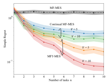
Figure 3: Synthetic optimization tasks: Simple regret (40) against the number of tasks, $n$, for MF-MES, Continual MF-MES $(\beta=0)$ with $V=5$ and $V=10$ particles, and MFT-MES ($\beta=1.2$) with $V=5$ and $V=10$ particles.

Fig. 3 shows the simple regret (40) as a function of the number of tasks $n$ observed so far. For MFT-MES, the weight parameter in (35) is set to $\beta=1.2$. Since MF-MES does not attempt to transfer knowledge across tasks, its average performance is constant for all values of $n$. By transferring knowledge across tasks, both Continual MF-MES and MFT-MES can reduce the simple regret as the number of observed tasks $n$ increases.

MFT-MES outperforms Continual MF-MES as soon as the number of tasks, $n$, is sufficiently large, here $n>2$. The advantage of Continual MF-MES for small values of $n$ is due to the fact that MF-MES focuses solely on the current task, while MFT-MES makes decisions also with the goal of improving performance on future tasks. In this sense, the price paid by MFT-MES to collect transferable knowledge is a minor performance degradation for the initial tasks. The benefits of the approach are, however, very significant for later tasks. For instance, at task $n=10$, MFT-MES decreases the simple regret by a factor of three as compared to Continual MF-MES when the number of particles is $V=10$.

It is also observed that increasing the number of particles $V$, is generally beneficial for both Continual MF-MES and MFT-MES. The performance gain with a larger $V$ can be ascribed to the larger capacity of retaining information about the uncertainty on the optimized parameter vector $\bm{\theta}$.

Fig. 4 demonstrates the impact of the weight parameter $\beta$ on the simple regret as a function of the number of tasks. Recall that the performance levels of MF-MES, as well as of Continual MF-MES, do not depend on the value of weight parameter $\beta$, which is an internal parameter of the MFT-MES acquisition function (35). The optimal value of $\beta$, which minimizes the simple regret, is marked with a star. It is observed that it is generally preferable to increase the value of $\beta$ as the number of tasks $n$ grows larger. This is because a larger $\beta$ favors the selection of input and fidelity level that focus on the performance of future tasks, and this provident approach is more beneficial for longer time horizons. For example, when the sequence of tasks is short, i.e., when $n\leq 2$, the choice $\beta=0$, i.e., Continual MF-MES attains best performance; while the weight parameter $\beta=1.2$ produces best performance given $n=9$ tasks in the sequence.

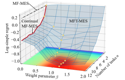
Figure 4: Synthetic optimization tasks: Log-simple regret against weight parameter $\beta$ and the number of tasks, $n$, for MF-MES (black dash-dotted line), Continual MF-MES (red solid line), and MFT-MES (blue surface). The optimal values of $\beta$ at the corresponding number of tasks $n$ are labeled as gold stars. The number of particles for Continual MF-MES and MFT-MES is set to $V=10$.

V-D Radio Resource Management

In this section, we study an application to wireless communications presented in [6, 7]. The problem involves optimizing parameters $\mathbf{x}$ that dictate the power allocation strategy of base stations in a cellular system. The vector $\mathbf{x}$ contains two parameters for each base station with the first parameter taking 114 possible values and the second parameter taking 8 possible values. Tasks are generated by randomly deploying users in a given geographical area of radius up to 200 meters, while restricting the users’ locations to change by no more than 10 meters for task $n$ as compared to the most recent task $n-1$.

The objective function $f_{n}(\mathbf{x})$ is the sum-spectral efficiency at which users transmit to the base stations. Evaluating the sum-spectral efficiency requires averaging out the randomness of the propagation channels, and the simulation costs determines the number of channel samples used to evaluate this average. Accordingly, we set the cost levels as $\lambda^{(1)}=10,\lambda^{(2)}=20,\lambda^{(3)}=50$, and $\lambda^{(4)}=100$, which measure the number of channel samples used at each fidelity level. The total query cost budget is set to $\Lambda=2000$ for every task.

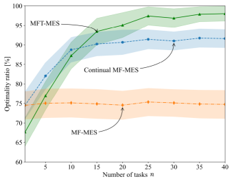
Figure 5: Radio resource management for wireless systems [7]: Optimality ratio (41) against the number of tasks, $n$, for MF-MES, Continual MF-MES ($\beta=0$), and MFT-MES ($\beta=1.6$) with $V=10$ particles.

We initialize the MFGP model (18) with 10 random evaluations across all fidelity levels, and the observation noise variance is $\sigma^{2}=0.83$. In a manner consistent with [7], the performance of each method is measured by the optimality ratio

$$\max\limits_{t=1,..,T_{n}}\frac{f^{(M)}_{n}(\mathbf{x}_{n,t})}{f_{n}^{*}},$$ (41)

which evaluates the best function of the optimal value $f_{n}^{*}$ attained during the optimization process. Finally, we set $V=10$ particles for Continual MF-MES and MFT-MES. All other experimental settings are kept the same as in Sec. V-B.

In Fig. 5, we set the weight parameter $\beta=1.6$ for MFT-MES and plot the optimality ratio (41) as a function of the number of tasks, $n$. Confirming the discussions in Sec. V-C, the performance of MF-MES is limited by the lack of information transfer across tasks. In contrast, the performance of both Continual MF-MES and MFT-MES benefits from information transfer. Furthermore, MFT-MES outperforms Continual MF-MES after processing 12 tasks. Through a judicious choice of input and fidelity levels targeting the shared parameters $\bm{\theta}$, at the end of 40-th task, MFT-MES provides, approximately, an $7\%$ gain in terms of optimality ratio over Continual MF-MES, and a $23\%$ gain over MF-MES.

The impact of the weight parameter $\beta$ used by MFT-MES on the performance evaluated at the 20-th and 40-th task is illustrated in Fig. 6. MFT-MES with any weight parameter $\beta>0$ outperforms all other schemes given the same number of tasks observed so far. The best performance of MFT-MES is obtained for $\beta=1.2$ at $n=20$ tasks, and for $\beta=1.6$ at $n=40$ tasks. Therefore, as discussed in Sec. V-C, a larger value of weight parameter $\beta$ is preferable as the number of tasks $n$ increases. Moreover, the performance of MFT-MES is quite robust to the choice of $\beta$. For instance, selecting larger weights $\beta$, up to $\beta=2.4$, is seen to yield a mild performance degradation as compared to the best settings of weight parameters $\beta=1.2$ for $n=20$ and $\beta=1.6$ for $n=40$.

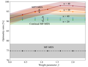
Figure 6: Radio resource management for wireless systems [7]: Optimality ratio (41) against weight parameter $\beta$, for MF-MES, Continual MF-MES with $n=20$ and $n=40$ tasks observed, and MFT-MES with $n=20$ and $n=40$ tasks observed. The number of particles for Continual MF-MES and MFT-MES is set to $V=10$.

V-E Gas Emission Source Term Estimation

Finally, we consider an application to the reverse problem formulation of gas emission source term estimation introduced in [36]. The problem aims to optimize a decision vector $\mathbf{x}$ that identifies the characteristics of the gas emission point source based on the Pasquill-Gifford dispersion model [55]. The feasible input domain of the vector is defined as $\mathbf{x}\in[10,5000]\times[-500,500]^{2}\times[0,10]\subset\mathbbm{R}^{4}$, with the first parameter being the source emission rate and the rest of the parameters describing the location of the emission source. Tasks are distinguished by the different locations of the sensors used to measure the concentration of emissions.

The objective function $f_{n}(\mathbf{x})$ is defined as the sum of the squared errors between the concentration measured at the sensors and the concentration calculated by the dispersion model given parameters $\mathbf{x}$. The fidelity of the evaluation of the objective function $f_{n}(\mathbf{x})$ depends on the atmospheric conditions, which can be classified into $M=6$ fidelity levels controlled by dispersion coefficients as in [36]. We set the cost levels as $\lambda^{(m)}=10+5\cdot(m-1)$; the total query cost budget is set to $\Lambda=750$ for every task; and the observation noise variance is set to $\sigma^{2}=10^{-3}$. The performance of all methods is measured by the simple regret in (40).

In Fig. 7, we set the weight parameter in (35) to $\beta=1.5$ for MFT-MES, and plot the simple regret (40) as a function of the number of tasks $n$ observed so far. The results demonstrate again the capacity of both Continual MF-MES and MFT-MES to transfer knowledge across tasks, achieving better performance as compared to MF-MES. After processing at least four tasks, MFT-MES outperforms Continual MF-MES. In particular, MFT-MES obtains a lower simple regret by a factor of two as compared to Continual MF-MES at the end of task $n=17$, confirming the importance of accounting for knowledge transfer in the acquisition function (35).

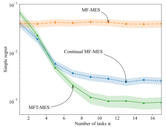
Figure 7: Gas emission source term estimation: Simple regret (40) against the number of tasks, $n$, for MF-MES, Continual MF-MES $(\beta=0)$, and MFT-MES ($\beta=1.5$) with $V=10$ particles.

In a manner similar to Sec. V-D, we demonstrate the impact of weight parameter $\beta$ on the simple regret evaluated at the 7-th and 17-th task in Fig. 8. The superiority of MFT-MES over all other schemes is observed to hold for any values of weight parameter $\beta>0$. MFT-MES achieves the best performance with weight parameter around $\beta=1.0$ for $n=7$, and approximately $\beta=1.5$ for $n=17$. The overall trend confirms the discussion in Sec. V-C, as a larger value of weight parameter $\beta$ is more desirable when the number of tasks $n$ increases.

VI Conclusion

In this work, we have have introduced MFT-MES, a novel information-theoretic acquisition function that balances the need to acquire information about the current task with goal of collecting information transferable to future tasks. The key mechanism underlying MFT-MES involves modeling transferable knowledge across tasks via shared inter-task latent variables, which are integrated into the acquisition function design and updated following Bayesian principles. From synthetic optimization tasks and real-world examples, we have demonstrated that the proposed MFT-MES scheme can obtain performance gains as large as an order of magnitude in terms of simple regret as compared to the state-of-art scheme that do not cater to the acquisition of transferable knowledge.

Future work may address theoretical performance guarantees in the forms of regret bounds to explain aspects such as the dependence of the optimal weight parameter $\beta$ used by MFT-MES as a function of the number of tasks and total query cost budget. Furthermore, it would be interesting to investigate the extensions to multi-objective multi-fidelity optimization problems [56]; the scalability to higher dimensions of the search space [57]; and the potential gains from incorporating generative models [58].

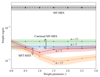
Figure 8: Gas emission source term estimation: Simple regret (40) against weight parameter $\beta$, for MF-MES, Continual MF-MES with $n=7$ and $n=17$ tasks observed, and MFT-MES with $n=7$ and $n=17$ tasks observed. The number of particles for Continual MF-MES and MFT-MES is set to $V=10$.

References

- [1] M. Zhang, H. Li, S. Pan, J. Lyu, S. Ling, and S. Su, “Convolutional neural networks-based lung nodule classification: A surrogate-assisted evolutionary algorithm for hyperparameter optimization,” IEEE Transactions on Evolutionary Computation, vol. 25, no. 5, pp. 869–882, 2021.
- [2] L. Demetrio, B. Biggio, G. Lagorio, F. Roli, and A. Armando, “Functionality-preserving black-box optimization of adversarial Windows malware,” IEEE Transactions on Information Forensics and Security, vol. 16, pp. 3469–3478, 2021.
- [3] J. Zhou, Z. Yang, Y. Si, L. Kang, H. Li, M. Wang, and Z. Zhang, “A trust-region parallel Bayesian optimization method for simulation-driven antenna design,” IEEE Transactions on Antennas and Propagation, vol. 69, no. 7, pp. 3966–3981, 2020.
- [4] H. B. Moss, V. Aggarwal, N. Prateek, J. González, and R. Barra-Chicote, “Boffin tts: Few-shot speaker adaptation by Bayesian optimization,” in Proceedings of IEEE International Conference on Acoustics, Speech and Signal Processing (ICASSP), 2020.
- [5] S. Xu, J. Li, P. Cai, X. Liu, B. Liu, and X. Wang, “Self-improving photosensitizer discovery system via Bayesian search with first-principle simulations,” Journal of the American Chemical Society, vol. 143, no. 47, pp. 19 769–19 777, 2021.
- [6] L. Maggi, A. Valcarce, and J. Hoydis, “Bayesian optimization for radio resource management: Open loop power control,” IEEE Journal on Selected Areas in Communications, vol. 39, no. 7, pp. 1858–1871, 2021.
- [7] Y. Zhang, O. Simeone, S. T. Jose, L. Maggi, and A. Valcarce, “Bayesian and multi-armed contextual meta-optimization for efficient wireless radio resource management,” IEEE Transactions on Cognitive Communications and Networking, vol. 9, no. 5, pp. 1282–1295, 2023.
- [8] Y. Wang, J. Fang, Y. Cheng, H. She, Y. Guo, and G. Zheng, “Cooperative end-edge-cloud computing and resource allocation for digital twin enabled 6G industrial iot,” IEEE Journal of Selected Topics in Signal Processing, pp. 1–14, 2023.
- [9] J. Johnston, X.-Y. Liu, S. Wu, and X. Wang, “A curriculum learning approach to optimization with application to downlink beamforming,” IEEE Transactions on Signal Processing, vol. 72, pp. 84–98, 2024.
- [10] R. Highfield and P. Coveney, “Virtual you: how building your digital twin will revolutionize medicine and change your life,” Princeton University Press, 2023.
- [11] J. Hoydis, F. A. Aoudia, S. Cammerer, M. Nimier-David, N. Binder, G. Marcus, and A. Keller, “Sionna rt: Differentiable ray tracing for radio propagation modeling,” arXiv preprint arXiv:2303.11103, 2023.
- [12] C. Ruah, O. Simeone, and B. Al-Hashimi, “A Bayesian framework for digital twin-based control, monitoring, and data collection in wireless systems,” IEEE Journal on Selected Areas in Communications, vol. 41, no. 10, pp. 3146–3160, 2023.
- [13] C. Ruah, O. Simeone, J. Hoydis, and B. Al-Hashimi, “Calibrating wireless ray tracing for digital twinning using local phase error estimates,” arXiv preprint arXiv:2312.12625, 2023.
- [14] W. Chen, W. Hong, H. Zhang, P. Yang, and K. Tang, “Multi-fidelity simulation modeling for discrete event simulation: An optimization perspective,” IEEE Transactions on Automation Science and Engineering, vol. 20, no. 2, pp. 1156–1169, 2022.
- [15] C. E. Rasmussen, Gaussian Processes in Machine Learning. Springer, 2004, pp. 63–71.
- [16] D. R. Jones, M. Schonlau, and W. J. Welch, “Efficient global optimization of expensive black-box functions,” Journal of Global optimization, vol. 13, pp. 455–492, 1998.
- [17] P. I. Frazier, W. B. Powell, and S. Dayanik, “A knowledge-gradient policy for sequential information collection,” SIAM Journal on Control and Optimization, vol. 47, no. 5, pp. 2410–2439, 2008.
- [18] Z. Wang, V. Y. Tan, and J. Scarlett, “Tight regret bounds for noisy optimization of a Brownian motion,” IEEE Transactions on Signal Processing, vol. 70, pp. 1072–1087, 2022.
- [19] Z. Wang and S. Jegelka, “Max-value entropy search for efficient Bayesian optimization,” in Proceedings of International Conference on Machine Learning, Sydney, Australia, 2017.
- [20] N. Srinivas, A. Krause, S. M. Kakade, and M. W. Seeger, “Information-theoretic regret bounds for Gaussian process optimization in the bandit setting,” IEEE Transactions on Information Theory, vol. 58, no. 5, pp. 3250–3265, 2012.
- [21] H. B. Moss, D. S. Leslie, J. Gonzalez, and P. Rayson, “Gibbon: General-purpose information-based Bayesian optimisation,” Journal of Machine Learning Research, vol. 22, no. 1, pp. 10 616–10 664, 2021.
- [22] K. Swersky, J. Snoek, and R. P. Adams, “Multi-task Bayesian optimization,” in Proceedings of Advances in Neural Information Processing Systems, Nevada, USA, 2013.
- [23] M. Poloczek, J. Wang, and P. Frazier, “Multi-information source optimization,” in Proceedings of Advances in neural information processing systems, California, USA, 2017.
- [24] R. Lam, D. L. Allaire, and K. E. Willcox, “Multifidelity optimization using statistical surrogate modeling for non-hierarchical information sources,” in Proceedings of 56th AIAA/ASCE/AHS/ASC Structures, Structural Dynamics, and Materials Conference, Florida, USA, 2015.
- [25] K. Kandasamy, G. Dasarathy, J. Schneider, and B. Póczos, “Multi-fidelity Bayesian optimisation with continuous approximations,” in Proceedings of International Conference on Machine Learning, Sydney, Australia, 2017.
- [26] J. Wu, S. Toscano-Palmerin, P. I. Frazier, and A. G. Wilson, “Practical multi-fidelity Bayesian optimization for hyperparameter tuning,” in Uncertainty in Artificial Intelligence, 2020.
- [27] P. Hennig and C. J. Schuler, “Entropy search for information-efficient global optimization.” Journal of Machine Learning Research, vol. 13, no. 6, 2012.
- [28] H. B. Moss, D. S. Leslie, and P. Rayson, “Mumbo: Multi-task max-value Bayesian optimization,” in Proceedings of Joint European Conference on Machine Learning and Knowledge Discovery in Databases, Ghent, Belgium, 2020.
- [29] S. Takeno, H. Fukuoka, Y. Tsukada, T. Koyama, M. Shiga, I. Takeuchi, and M. Karasuyama, “Multi-fidelity Bayesian optimization with max-value entropy search and its parallelization,” in Proceedings of International Conference on Machine Learning, 2020.
- [30] P. Mikkola, J. Martinelli, L. Filstroff, and S. Kaski, “Multi-fidelity Bayesian optimization with unreliable information sources,” in Proceedings of International Conference on Artificial Intelligence and Statistics, Valencia, Spain, 2023.
- [31] O. Vinyals, C. Blundell, T. Lillicrap, D. Wierstra et al., “Matching networks for one shot learning,” in Proceedings of Advances in Neural Information Processing Systems, vol. 29, Barcelona, Spain, 2016.
- [32] Y. Zhang, J. Jordon, A. M. Alaa, and M. van der Schaar, “Lifelong Bayesian optimization,” arXiv preprint arXiv:1905.12280, 2019.
- [33] J. Rothfuss, C. Koenig, A. Rupenyan, and A. Krause, “Meta-learning priors for safe Bayesian optimization,” in Proceedings of Conference on Robot Learning, Georgia, USA, 2023.
- [34] Q. Liu and D. Wang, “Stein variational gradient descent: A general purpose Bayesian inference algorithm,” Proceedings of Advances in Neural Information Processing Systems, Barcelona, Spain, 2016.
- [35] L. C. W. Dixon, “The global optimization problem: an introduction,” Towards Global Optimiation 2, pp. 1–15, 1978.
- [36] H. Li and J. Zhang, “Fast source term estimation using the PGA-NM hybrid method,” Engineering Applications of Artificial Intelligence, vol. 62, pp. 68–79, 2017.
- [37] B. Lei, T. Q. Kirk, A. Bhattacharya, D. Pati, X. Qian, R. Arroyave, and B. K. Mallick, “Bayesian optimization with adaptive surrogate models for automated experimental design,” Npj Computational Materials, vol. 7, no. 1, p. 194, 2021.
- [38] G. Malkomes, C. Schaff, and R. Garnett, “Bayesian optimization for automated model selection,” in Proceedings of Advances in Neural Information Processing Systems, Barcelona, Spain, 2016.
- [39] A. I. Forrester, A. Sóbester, and A. J. Keane, “Multi-fidelity optimization via surrogate modelling,” Proceedings of the royal society a: mathematical, physical and engineering sciences, vol. 463, no. 2088, pp. 3251–3269, 2007.
- [40] L. Le Gratiet and J. Garnier, “Recursive co-kriging model for design of computer experiments with multiple levels of fidelity,” International Journal for Uncertainty Quantification, 2014.
- [41] J. Rothfuss, V. Fortuin, M. Josifoski, and A. Krause, “PACOH: Bayes-optimal meta-learning with PAC-guarantees,” in Proceedings of International Conference on Machine Learning, 2021.
- [42] E. V. Bonilla, K. Chai, and C. Williams, “Multi-task Gaussian process prediction,” in Proceedings of Advances in Neural Information Processing Systems, Vancouver, Canada, 2007.
- [43] J. Gardner, G. Pleiss, K. Q. Weinberger, D. Bindel, and A. G. Wilson, “Gpytorch: Blackbox matrix-matrix Gaussian process inference with gpu acceleration,” in Proceedings of Advances in Neural Information Processing Systems, Montreal, Canada, 2018.
- [44] M. C. Kennedy and A. O’Hagan, “Predicting the output from a complex computer code when fast approximations are available,” Biometrika, vol. 87, no. 1, pp. 1–13, 2000.
- [45] M. A. Alvarez and N. D. Lawrence, “Computationally efficient convolved multiple output Gaussian processes,” Journal of Machine Learning Research, vol. 12, pp. 1459–1500, 2011.
- [46] T. M. Cover and J. A. Thomas, Elements of Information Theory. (Wiley Series in Telecommunications and Signal Processing), 2nd ed. New York, NY, USA: Wiley, 2006.
- [47] A. Damianou and N. D. Lawrence, “Deep Gaussian processes,” in Proceedings of International Conference on Artificial Intelligence and Statistics, Arizona, USA, 2013.
- [48] S. J. Sloman, A. Bharti, and S. Kaski, “The fundamental dilemma of Bayesian active meta-learning,” arXiv preprint arXiv:2310.14968, 2023.
- [49] N. A. Weiss, P. T. Holmes, and M. Hardy, A course in probability. Pearson Addison Wesley Boston, MA, USA:, 2006.
- [50] K. Moshksar and A. K. Khandani, “Arbitrarily tight bounds on differential entropy of Gaussian mixtures,” IEEE Transactions on Information Theory, vol. 62, no. 6, pp. 3340–3354, 2016.
- [51] F. Nielsen and K. Sun, “Guaranteed bounds on information-theoretic measures of univariate mixtures using piecewise log-sum-exp inequalities,” Entropy, vol. 18, no. 12, p. 442, 2016.
- [52] O. Simeone, Machine learning for engineers. Cambridge university press, 2022.
- [53] C. M. Bishop and N. M. Nasrabadi, Pattern recognition and machine learning. Springer, 2006, vol. 4.
- [54] S. Bubeck, R. Munos, and G. Stoltz, “Pure exploration in multi-armed bandits problems,” in Proceedings of International Conference on Algorithmic Learning Theory, Porto, Portugal, 2009.
- [55] D. A. Crowl and J. F. Louvar, Chemical process safety: fundamentals with applications. Pearson Education, 2001.
- [56] H. Li, Y. Jin, and T. Chai, “Evolutionary multi-objective Bayesian optimization based on multisource online transfer learning,” IEEE Transactions on Emerging Topics in Computational Intelligence, vol. 8, no. 1, pp. 488–502, 2024.
- [57] W. J. Maddox, M. Balandat, A. G. Wilson, and E. Bakshy, “Bayesian optimization with high-dimensional outputs,” in Proceedings of Advances in Neural Information Processing Systems, 2021.
- [58] Z. Liang, Y. Zhu, X. Wang, Z. Li, and Z. Zhu, “Evolutionary multitasking for multi-objective optimization based on generative strategies,” IEEE Transactions on Evolutionary Computation, vol. 27, no. 4, pp. 1042–1056, 2023.