Non-Hermitian Persistent Current Transport

Abstract

Persistent currents circulate continuously without requiring external power sources. Here, we extend their theory to include dissipation within the framework of non-Hermitian quantum Hamiltonians. Using Green’s function formalism, we introduce a non-Hermitian Fermi-Dirac distribution and derive an analytical expression for the persistent current that relies solely on the complex spectrum. We apply our formula to two dissipative models supporting persistent currents: ($i$) a phase-biased superconducting-normal-superconducting junction; ($ii$) a normal ring threaded by a magnetic flux. We show that the persistent currents in both systems exhibit no anomalies at any emergent exceptional points, whose signatures are only discernible in the current susceptibility. We validate our findings by exact diagonalization and extend them to account for finite temperatures and interaction effects. Our formalism offers a general framework for computing quantum many-body observables of non-Hermitian systems in equilibrium, with potential extensions to non-equilibrium scenarios.

Introduction.—Recent intensive research in non-Hermitian (NH) physics [1, 2, 3, 4] has revealed intriguing phenomena in both the classical [5, 6, 7, 8, 9] and quantum realms [10, 11, 12]. The concept of the generalized Brillouin zone has reshaped the conventional bulk-edge correspondence [13, 14, 15], while the symmetry classifications of the NH matrices have enriched the topological phases compared to their Hermitian counterparts [16, 17, 18, 19]. Exceptional points (EPs), where the NH Hamiltonian is not diagonalizable [20, 21, 22], can enhance sensing capabilities in optical microcavities [23, 24, 25, 26], and also trigger new critical phenomena in spin chains [27, 28, 29].

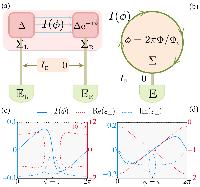
Figure 1: Schematic of systems coupled to external reservoirs $\mathbb{E}$: (a) an SNS junction with a phase bias $\phi$; (b) a normal metallic ring threaded by normalized magnetic flux $\phi$. Each system is characterized by an effective NH Hamiltonian $\mathcal{H}_{\rm eff}$ that includes a complex self-energy $\Sigma$ from $\mathbb{E}$. In equilibrium, both models maintain persistent currents $I(\phi)$ and zero leakage currents $I_{\textsc{e}}$. (c) and (d) Complex spectra $\varepsilon_{\pm}$ showing EPs around $\pi$ (black lines) and persistent current $I(\phi)$ as a function of $\phi$. The current $I(\phi)$ calculated using Eq. (1) shows no signs of singularity at the EPs. Parameters: (c) $N_{\textsc{l}}=N_{\textsc{m}}=N_{\textsc{r}}=4$, $N_{\textsc{e}}=101$, $t=-\Delta=-1$, $\kappa=0.4t$, $\mu=g=-1.1$; (d) $N=6$, $N_{\textsc{e}}=101$, $t=\kappa=\mu=-1$, $g=0$, $t_{i}\sim t*\mathrm{Unif}(0.7,1.3)$.

In the field of open quantum systems, NH physics is instrumental in characterizing the dissipative nature of systems [30, 31, 32]. The Lindblad formalism [33, 34, 35, 36] provides routes to address system-reservoir interactions. By neglecting quantum jumps or focusing on Gaussian systems [37, 38, 39], the dynamics is dictated solely by an effective NH Hamiltonian $\mathcal{H}_{\rm eff}$. The Green’s function formalism presents an alternative path to $\mathcal{H}_{\rm eff}$ by integrating out external reservoirs $\mathbb{E}$ to include complex self-energies $\Sigma\neq\Sigma^{\dagger}$ [40, 41, 42, 43]. Although the spectral properties of $\mathcal{H}_{\rm eff}$ have been extensively explored, quantum many-body observables, such as the supercurrents in phase-biased superconducting-normal-superconducting (SNS) junctions shown in Fig. 1(a), are currently under active discussion. Existing approaches, such as the derivative of complex eigenvalues [44, 45] and the expectation values obtained from the left-right (LR) or right-right (RR) eigenvectors [46], often yield anomalies at EPs, calling for a microscopic approach to grasp the subtleties of the NH persistent current transport.

In this work, we provide a resolution to this conundrum grounded on a NH Fermi-Dirac distribution associated with the biorthogonal single-particle eigenstates. We find that the supercurrent $I(\phi)$ in an SNS junction biased by a phase $\phi$ and coupled to reservoirs is given by (in units of $e/\hbar$):

$$I(\phi)=-\frac{1}{\pi}\frac{\mathrm{d}}{\mathrm{d}\phi}\mathrm{Im}\mathrm{Tr}(\mathcal{H}_{\rm eff}\ln\mathcal{H}_{\rm eff})\,.$$ (1)

This formula is non-perturbative and can also accurately describe the strong coupling regime. Moreover, it also applies to the persistent current in a normal mesoscopic ring threaded by a magnetic flux, as shown in Fig. 1(b). Our results align with the exact diagonalization of the full Hermitian system including the reservoir and do not exhibit any singularities at EPs for both models [see Fig. 1(c) and (d)]. We further generalize Eq. (1) to finite temperatures and find that persistent currents are reduced, which is also observed when many-body interactions are taken into account. Finally, we show that the signatures of EPs can instead be revealed in the current susceptibility associated with response to a $ac$ phase bias drive. Our formalism not only clarifies the behavior of persistent currents in fermionic NH systems but also sets the stage for analyzing other quantum many-body observables with dissipation.

Phenomenology and methodology.—Initially, we outline a heuristic explanation of our main findings, deferring the technical details to subsequent sections and the Supplemental Material (SM) [47]. We focus, for simplicity, on spinless fermionic systems with Hamiltonians that depend on a parameter $\phi$, such as in phase-biased SNS junctions $H_{\rm sys}(\phi)=\vec{C}^{\dagger}\mathcal{H}_{\rm sys}(\phi)\vec{C}/\mathbf{2}$, where $\mathcal{H}_{\rm sys}(\phi)$ is the Bogoliubov-de Gennes (BdG) Hamiltonian, $\vec{C}=(c_{1},\dots,c_{\textsc{n}},c^{\dagger}_{1},\dots,c^{\dagger}_{\textsc{n}})^{\textsc{t}}$ is a $\mathbf{2}N$-dimensional spinor, and $c_{j}^{\dagger}$ ($c_{j}$) is the fermionic creation (annihilation) operator at site $j$. The discussion below also applies to normal metals described by $\mathcal{H}_{\rm sys}(\phi)$ on an $N$-dimensional basis $\vec{C}=(c_{1},\dots,c_{\textsc{n}})^{\textsc{t}}$, substituting $\mathbf{2}$ for $\mathbf{1}$. For brevity, we will use calligraphy to denote the first quantized operators and omit the explicit dependence on $\phi$ in our notation for Hamiltonians, eigenvalues, and eigenvectors hereafter.

For isolated and Hermitian systems $\mathcal{H}_{\rm sys}$, the persistent current $I_{\rm iso}(\phi)$ in the many-body ground state $E_{0}$ follows [48],

$$I_{\rm iso}(\phi)=\mathbf{2}\frac{\mathrm{d}E_{0}}{\mathrm{d}\phi}=\sum_{\epsilon_{n}\leqslant 0}\frac{\mathrm{d}\epsilon_{n}}{\mathrm{d}\phi}=\sum_{\epsilon_{n}\leqslant 0}\frac{\braket{\psi_{n}}{\mathcal{J}}{\psi_{n}}}{\mathbf{2}}\,,$$ (2)

where the factor of two stems from the Cooper pair, $J=\vec{C}^{\dagger}\mathcal{J}\vec{C}/\mathbf{2}$ is the persistent current operator, $\epsilon_{n}$ and $\ket{\psi_{n}}$ are eigenvalues and eigenstates of $\mathcal{H}_{\rm sys}$. Given the local conservation law of $n_{j}=c^{\dagger}_{j}c_{j}$ in the $\mathbb{N}$ segment (e.g., the normal part in SNS junctions), the site-resolved current operator [32], $J_{j}=-\mathrm{i}t_{j}(c^{\dagger}_{j}c_{j+1}-c^{\dagger}_{j+1}c_{j})$, follows the continuity equation: $0=\dot{n}_{j}=\mathrm{i}[H_{\rm sys},n_{j}]=J_{j}-J_{j-1},\forall j\in\mathbb{N}$, where $t_{j}$ is the hopping strength at site $j$. Therefore, we set $J\equiv J_{j}$ at the first site of $\mathbb{N}$ and omit the subscript.

To account for dissipation, we posit that the system is coupled to a thermal reservoir $\mathbb{E}$, leading to the emergence of a complex self-energy $\Sigma(\omega)$ within the system. In the wide band limit $\Sigma(\omega)\approx\Sigma(0)$ [32], the system is effectively described by the NH Hamiltonian $\mathcal{H}_{\rm eff}\equiv\mathcal{H}_{\rm sys}+\Sigma(0)$, which exhibits a complex spectrum $\varepsilon_{n}$ with $\mathrm{Im}\,\varepsilon_{n}\leqslant 0$ and supports biorthogonal single-particle modes [49]: $\mathcal{H}_{\rm eff}\ket{\psi^{\textsc{r}}_{n}}=\varepsilon_{n}\ket{\psi^{\textsc{r}}_{n}}$, $\mathcal{H}_{\rm eff}^{\dagger}\ket{\psi^{\textsc{l}}_{n}}=\varepsilon^{*}_{n}\ket{\psi^{\textsc{l}}_{n}}$, and $\braket{\psi^{\textsc{l}}_{n}}{\psi^{\textsc{r}}_{m}}=\delta_{nm}$. Using this biorthogonal basis, we represent the retarded Green’s function of the system as [50]

$$G_{\rm sys}(\omega)=\frac{1}{\omega-\mathcal{H}_{\rm eff}}=\sum_{n}\frac{\ket{\psi^{\textsc{r}}_{n}}\bra{\psi^{\textsc{l}}_{n}}}{\omega-\varepsilon_{n}}\,,$$ (3)

and obtain the density of states operator $\rho(\omega)=\mathrm{i}[G_{\rm sys}(\omega)-G^{\dagger}_{\rm sys}(\omega)]/2\pi$. In thermal equilibrium, any correlator can be calculated by $\braket{c^{\dagger}_{i}c_{j}}=\int\braket{j}{\rho(\omega)}{i}f_{\textsc{fd}}(\omega)\mathrm{d}\omega$, where $f_{\textsc{fd}}(\omega)$ is the Fermi-Dirac distribution of the entire system. Given $f_{\textsc{fd}}(\omega)=\Theta(-\omega)$ at zero temperature, we derive an analytic correlator $\braket{c^{\dagger}_{i}c_{j}}$ by integrating over $\omega$:

$$\braket{c^{\dagger}_{i}c_{j}} =\frac{\mathrm{i}}{2\pi}\sum_{n}\left(\psi^{\textsc{l*}}_{ni}\psi^{\textsc{r}}_{nj}\ln\varepsilon_{n}-\psi^{\textsc{r*}}_{ni}\psi^{\textsc{l}}_{nj}\ln\varepsilon^{*}_{n}\right)\,,$$ (4)

where $\psi^{\textsc{l/r}}_{nj}\equiv\braket{j}{\psi^{\textsc{l/r}}_{n}}$, $\ln\varepsilon_{n}\equiv\ln|\varepsilon_{n}|+\mathrm{i}\arg\varepsilon_{n}$ and $-\pi\leqslant\arg\varepsilon_{n}\leqslant 0$ . Similarly, $\braket{c_{i}c_{j}}$ is obtained by replacing $i$ with $N+i$ on the right-hand side of Eq. (4). Therefore, the expectation value of a quadratic Hermitian operator $O=\vec{C}^{\dagger}\mathcal{O}\vec{C}/\mathbf{2}$ is [47]

$$\braket{O}=\mathrm{Im}\sum_{n}\frac{\braket{\mathcal{O}}^{\textsc{lr}}_{n}f_{\rm eff}(\varepsilon_{n})}{\mathbf{2}}=\frac{\mathrm{Im}\mathrm{Tr}[\mathcal{O}f_{\rm eff}(\mathcal{H}_{\rm eff})]}{\mathbf{2}}\,,$$ (5)

where $\braket{\mathcal{O}}^{\textsc{lr}}_{n}\equiv\braket{\psi^{\textsc{l}}_{n}}{\mathcal{O}}{\psi^{\textsc{r}}_{n}}$ and $f_{\rm eff}(\varepsilon)\equiv-(1/\pi)\ln\varepsilon$ acts as a Fermi-Dirac distribution for NH systems, whose imaginary part reduces to $\Theta(-\varepsilon)$ as $\mathrm{Im}\,\varepsilon\rightarrow 0$. Eq. (5) represents one of our main results. The persistent current $I(\phi)$ can be calculated by substituting $\mathcal{O}$ with $\mathcal{J}$ in Eq. (5). Furthermore, applying the identity $\braket{\mathcal{J}}^{\textsc{lr}}_{n}=\mathbf{2}\partial_{\phi}\varepsilon_{n}$ for each biorthogonal single-particle mode and rearranging the derivatives, one can obtain Eq. (1) and verify that it recovers Eq. (2) in the Hermitian limit (see SM [47] for details). It is important to emphasize that our Eq. (1) is distinct from a simple continuation of Eq. (2) to complex eigenvalues $\sum_{\mathrm{Re}\,\varepsilon_{n}\leqslant 0}\partial_{\phi}\varepsilon_{n}$ (or equivalently the LR-basis current $I_{\textsc{lr}}(\phi)\equiv\sum_{\mathrm{Re}\,\varepsilon_{n}\leqslant 0}\braket{\mathcal{J}}^{\textsc{lr}}_{n}/\mathbf{2}$) recently proposed in Refs. [44, 45, 46], as well as the RR-basis current $I_{\textsc{rr}}(\phi)\equiv\sum_{\mathrm{Re}\,\varepsilon_{n}\leqslant 0}\braket{\mathcal{J}}^{\textsc{rr}}_{n}/\mathbf{2}$ widely adopted with post-selection [52, 53, 54]. As demonstrated below, both of these definitions fail to accurately describe the persistent current in equilibrium, whereas Eq. (1) is in full agreement with the exact diagonalization.

Model reservoir and self-energy.—To validate our findings, we connect the system $H_{\rm sys}$ to a $N_{\textsc{e}}$-site fermionic reservoir $H_{\rm res}=\sum\nolimits_{j}\big{[}(tc^{\dagger}_{j}c_{j+1}+{\rm H.c.})+gc^{\dagger}_{j}c_{j}\big{]}$, where $t<0$ is the hopping strength and $g$ is the chemical potential. This specific reservoir is chosen for its dual analytical and numerical merits. First, connecting one end of $\mathbb{E}$ to the $l$-site of the system via $H_{\rm tun}=\kappa(c^{\dagger}_{N_{\textsc{e}}}c_{l}+c^{\dagger}_{l}c_{N_{\textsc{e}}})$ with coupling strength $\kappa<0$ will induce a self-energy $\Sigma_{l}(0)=\Sigma(0)\otimes\ket{l}\bra{l}$ onto $\mathcal{H}_{\rm sys}$, where $\Sigma(0)=-\kappa^{2}/t^{2}(\tau_{z}g/2+\mathrm{i}\sqrt{t^{2}-(g/2)^{2}})$ and $\tau_{z}$ is the Pauli-$Z$ matrix acting in the particle-hole space [31]. This expression is exact when $N_{\textsc{e}}\rightarrow\infty$ and also applies to normal metals upon removal of $\tau_{z}$ [47]. Second, the tight-binding form of $H_{\rm res}$ allows us to compare Eqs. (1) and (2) by performing an exact diagonalization of the entire Hermitian system $H_{\rm tot}=H_{\rm sys}+H_{\rm res}+H_{\rm tun}$. Next, we apply this benchmark framework to two concrete NH models: a phase-biased SNS junction and a normal ring threaded by a magnetic flux.

NH SNS junctions.—The SNS junction is a pivotal platform for quantum transport, whose Hamiltonian reads

$$\mkern-8.0muH_{\textsc{sns}}\mkern-5.0mu=\mkern-5.0mu\sum\nolimits_{j}\mkern-4.0mu(t_{j}c^{\dagger}_{j}c_{j+1}+\Delta_{j}\mathrm{e}^{-\mathrm{i}\phi_{j}}c^{\dagger}_{j}c^{\dagger}_{j+1}+\mkern-2.0mu\mathrm{H.c.})\mkern-2.0mu+\mkern-2.0mu\mu c^{\dagger}_{j}c_{j}\,,$$ (6)

where $\Delta_{j}$ is the superconducting gap with phase $\phi_{j}$ at site $j$, $\mu$ is the chemical potential and $t_{j}=t$. The number of sites in the left, middle and right parts is $N_{\textsc{l}},N_{\textsc{m}},N_{\textsc{r}}$, respectively. The middle segment is normal metal by setting $\Delta_{j}=\phi_{j}=0$, $\forall j\in\mathbb{N}\equiv[N_{\textsc{l}},N_{\textsc{l}}+N_{\textsc{m}}]$. The outer segments are superconductors $\Delta_{j}=\Delta\neq 0$ with phase bias applied such that $\phi_{j}=\phi$ in the right segment and $\phi_{j}=0$ in the left segment.

As depicted in Fig. 1(a), the SNS junction incorporates self-energies $\Sigma_{\textsc{l}}=\Sigma_{1}(0)$ and $\Sigma_{\textsc{r}}=\Sigma_{\textsc{n}}(0)$, after being connected to two separate reservoirs at its ends. This results in an effective NH Hamiltonian $\mathcal{H}_{\rm eff}=\mathcal{H}_{\textsc{sns}}+\Sigma_{\textsc{l}}+\Sigma_{\textsc{r}}$, whose spectrum exhibits pairs $(+\varepsilon_{n},-\varepsilon^{*}_{n})$ pertaining to the particle-hole symmetry of NH systems [17]. Fig. 1(c) highlights a pair of complex spectra $\varepsilon_{\pm}$ with EPs near $\phi=\pi$, where $\mathrm{Re}\,\varepsilon_{\pm}$ are pinned to zero. The calculation of supercurrents in the presence of EPs has recently garnered attention and sparked ongoing debates. As mentioned above, considering $\braket{\mathcal{J}}^{\textsc{lr}}_{n}=\mathbf{2}\partial_{\phi}\varepsilon_{n}$, a simple generalization of Eq. (2) to complex eigenvalues $\sum_{\mathrm{Re}\,\varepsilon_{n}\leqslant 0}\partial_{\phi}\varepsilon_{n}$ [44, 45] is equivalent to the LR-basis current $I_{\textsc{lr}}(\phi)$ [46]. However, as shown in Fig. 2(a), this approach results in a divergent supercurrent due to the non-differentiable nature of EPs. On the other hand, the RR-basis current $I_{\textsc{rr}}(\phi)$ has a finite but non-smooth value at EPs, and also exhibits asymmetry around $\pi$. Furthermore, $I_{\textsc{rr}}(\phi)$ does not adhere to the local conservation law and will show distinct curves for different $j\in\mathbb{N}$ (see SM [47] for details). In stark contrast, the current $I(\phi)$ computed by Eq. (1) exhibits no anomalies at EPs. It matches excellently with the current calculated from Eq. (2) by exact diagonalization for the entire Hermitian $H_{\rm tot}$ with a large reservoir. Compared to current $I_{\rm iso}(\phi)$ in an isolated SNS junction, we observe an enhancement in $I(\phi)$ within the moderate coupling regime $\kappa=0.4t$. This seemingly counterintuitive effect arises because the lower-energy mode $\varepsilon_{-}$ has a negative contribution to the current, which is effectively balanced by $\varepsilon_{+}$ due to level broadening in the NH case. However, as $\kappa/t$ increases, $I(\phi)$ starts to decrease, since dissipation also suppresses the positive current contribution from other states [47].

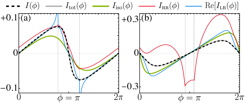
Figure 2: Methodological comparisons of persistent currents in two NH systems: (a) a phase-biased SNS junction; (b) a normal ring threaded by a magnetic flux. The current $I(\phi)$ (dashed) computed by Eq. (1) matches the exact diagonalization (gray) of the full Hermitian system. The isolated system (green) acts as a reference, showing an enhanced (reduced) current for the SNS (ring) model upon coupling to reservoirs. In (a), LR-basis currents (blue) diverge at the EPs (black lines), a feature not observed in (b), where a pair of EP-modes $\varepsilon_{\pm}$ cancel out the divergence. RR-basis currents (red) violate the local conservation law and exhibit asymmetry around $\pi$. The parameters are the same as in Fig. 1.

NH normal rings.—A mesoscopic ring threaded by a magnetic flux $\Phi$ also carries a persistent current because the coherence length of the wavefunction extends over its entire circumference [55, 56, 57, 58]. The gauge-invariant tight-binding Hamiltonian is given by [59, 60, 61]:

$$H_{\rm ring}= \sum\nolimits_{j}(t_{j}\mathrm{e}^{-\mathrm{i}\phi_{j}}c^{\dagger}_{j}c_{j+1}+\mathrm{H.c.})+\mu c^{\dagger}_{j}c_{j}\,,$$ (7)

where the normalized magnetic flux $\phi_{N}=\phi=2\pi\Phi/\Phi_{0}$ is placed between the $N$-th and first site, leaving other $\phi_{j}=0$. Here, $\Phi_{0}=h/e$ is the flux quantum that reflects the periodicity of Eq. (7) in the flux $\Phi$ [62]. We account for elastic scatterings by assigning uniformly random hopping strengths along the ring . However, since the local conservation law spans the whole ring, $\braket{J_{j}}$ remains uniform across all sites.

As illustrated in Fig. 1(b), the fermionic reservoir is connected to a single site within the ring [64], inducing a self-energy $\Sigma\equiv\Sigma_{\textsc{n}}(0)$. Consequently, the ring is described by $\mathcal{H}_{\rm eff}=\mathcal{H}_{\rm ring}+\Sigma$. When $\mu=0$, similar to the SNS junctions, the LR-basis current $I_{\textsc{lr}}(\phi)$ of the ring will diverge at EPs near $\phi=\pi$. Here, in order to explore different impacts of EPs, we set $\mu=-1$ and shift two EP-modes $\varepsilon_{\pm}$ below the Fermi level, as depicted in Fig. 1(d). Since $\varepsilon_{\pm}$ contribute to $I_{\textsc{lr}}(\phi)$ in pairs, their divergences cancel out, resulting in a smooth curvature for $I_{\textsc{lr}}(\phi)$ in Fig. 2(b). The RR-basis current $I_{\textsc{rr}}(\phi)$ violates the local conservation law and exhibits a non-sinusoidal curve due to inhomogeneous hopping strengths. Neither of these approaches can accurately describe the persistent current $I(\phi)$. However, the current $I(\phi)$ calculated using Eq. (1) aligns with exact diagonalization results that include a large reservoir. Compared to the current in the isolated ring, $I(\phi)$ is reduced because the positive current contributions from single-particle modes are diluted by dissipation-induced level broadening [65]. These conclusions remain consistent regardless of the number of reservoirs.

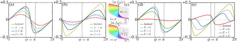
Figure 3: Effects of temperature and interactions on persistent currents $I(\phi)$ in NH systems. Panels (a) and (b) display $I(\phi)$ at finite temperatures $\beta=1/k_{\textsc{b}}T$ for an SNS junction and a mesoscopic ring, compared to isolated systems at $T=0$ (green). The currents computed using Eq. (9) (dashed) are consistent with the exact diagonalization (solid), indicating a decrease in $I(\phi)$ as $T$ increases. (c) Illustration of the imaginary part of the NH Fermi-Dirac distribution at zero and finite temperatures, where $\mathrm{Im}\,f_{\rm eff}(\varepsilon,\beta)$ in Eq. (8) will reduce to the conventional Fermi-Dirac distribution (dashed) as $\mathrm{Im}\,\varepsilon\rightarrow 0$. In (d) and (e), many-body interactions are shown to suppress the amplitude of $I(\phi)$ in both systems. The parameters are as in Fig. 1. No singularities are found at EPs (black lines) in all cases presented.

Finite temperature and interaction effects.—First, we consider the effect of thermal fluctuations on the persistent current . This requires integrating the density of states $\rho(\omega)$ over $\omega$ using $f_{\textsc{fd}}(\omega,\beta)=1/(\mathrm{e}^{\beta\omega}+1)$ and subsequently extending $f_{\rm eff}(\varepsilon)$ in Eq. (5) to form an effective NH Fermi-Dirac distribution at finite temperatures:

$$f_{\rm eff}(\varepsilon,\beta)=-\frac{1}{\pi}\left[\Psi\left(\frac{1}{2}+\frac{\mathrm{i}\beta\varepsilon}{2\pi}\right)-\frac{\mathrm{i}\pi}{2}\right]\,.$$ (8)

Above, $\beta=1/k_{\textsc{b}}T$, $k_{\textsc{b}}$ is the Boltzmann constant, and $\Psi$ is the digamma function [67]. Using Eq. (8), we find that at finite temperatures, Eq. (1) becomes (see SM [47] for details):

$$I(\phi,\beta)=\frac{2}{\beta}\frac{\mathrm{d}}{\mathrm{d}\phi}\mathrm{Re}\,\mathrm{Tr}\,\mathrm{log\Gamma}\left(\frac{1}{2}+\frac{\mathrm{i}\beta}{2\pi}\mathcal{H}_{\rm eff}\right)\,,$$ (9)

where $\mathrm{log\Gamma}$ is the log gamma function [68]. Eq. (9) extends the expression $\mathbf{2}\partial_{\phi}F$ for the persistent current, where $F$ denotes the free energy in Hermitian systems [48], to encompass NH scenarios. As shown in Fig. 3(a) and (b), Eq. (9) includes Eq. (1) when at $T=0$ and accurately matches the currents for $T\neq 0$ calculated by exact diagonalization. This indicates a decrease in currents for both systems as $T$ increases. As illustrated in Fig. 3(c), such an excellent agreement is grounded on the fact that $\mathrm{Im}\,f_{\rm eff}(\varepsilon,\beta)$ in Eq. (8) will revert to $f_{\textsc{fd}}(\varepsilon,\beta)$ as $\mathrm{Im}\,\varepsilon\rightarrow 0$. The smoothness of persistent currents near EPs can be attributed to the analytic properties of $f_{\rm eff}(\varepsilon,\beta)$ in the lower complex plane [47].

To examine potential characteristics of EPs in the presence of many-body interactions, we introduce the electrostatic repulsion $H_{\rm int}=U\sum_{j\in\mathbb{N}}(n_{j}-1/2)(n_{j+1}-1/2)$, where $U$ is the interaction strength. In such interacting scenarios, the first equality in Eq. (2) remains valid for the ground state. To maintain each reservoir as large as $N_{\textsc{e}}=101$, we perform the density matrix renormalization group (DMRG) algorithm via DMRGpy [69]. Fig. 3(d)(e) show that as $U$ increases, the amplitude of $I(\phi)$ in both systems will eventually be suppressed to zero due to the enhanced electron-electron scattering . No signatures of EPs are detected in the current in any of the cases presented with respect to temperatures and interactions.

Current susceptibility.—To elucidate the presence of EPs in systems with a phase-dependent spectrum, here we derive their linear response to a time-dependent phase driving $\phi(\tau)=\phi+\delta\phi(\tau)$, with $\delta\phi(\tau)\ll 1$. The current susceptibility that characterizes the response is given by [71, 72, 73]:

$$\Pi(\phi,\tau) =-\mathrm{i}\Theta(\tau)\braket{[J(\tau),J(0)]}\,.$$ (10)

We first transform Eq. (10) to the frequency space $\Pi(\phi,\omega)=\int\Pi(\phi,\tau)\mathrm{e}^{+\mathrm{i}\omega\tau}\mathrm{d}\tau$ and use the biorthogonal modes to obtain

$$\mathrm{Im}\,\Pi(\phi,\omega) =\pi t_{j}^{2}\,\mathrm{Re}[\mathbb{P}(\phi,+\omega)-\mathbb{P}(\phi,-\omega)]\,,$$

$$\mathbb{P}(\phi,\omega) =P_{j+1,j,j+1,j}(\omega)-P_{j,j,j+1,j+1}(\omega)$$

$$+P_{j,j+1,j,j+1}(\omega)-P_{j+1,j+1,j,j}(\omega)\,,$$ (11)

with $P_{ijkl}(\omega)\equiv\int\braket{i}{\rho(\omega^{\prime})}{j}\braket{k}{\rho(\omega+\omega^{\prime})}{l}f_{\textsc{fd}}(\omega^{\prime})\mathrm{d}\omega^{\prime}$. In the case of SNS junctions, $\mathbb{P}(\phi,\omega)$ contains four additional terms stemming from the contributions of the holes . Nevertheless, the integral $P_{ijkl}(\omega)$ is shared by both systems and possesses an analytical expression at $T=0$:

$$P_{ijkl}(\omega)=\sum_{nm}\frac{p^{nm-}_{ijkl}+p^{n\tilde{m}+}_{ijkl}+p^{\tilde{n}m-}_{ijkl}+p^{\tilde{n}\tilde{m}+}_{ijkl}}{4}\,,$$ (12)

$$p^{nm\pm}_{ijkl}\equiv\psi^{\textsc{r}}_{ni}\psi^{\textsc{l*}}_{nj}\psi^{\textsc{r}}_{mk}\psi^{\textsc{l*}}_{ml}\frac{f_{\rm eff}(\pm\varepsilon_{n})-f_{\rm eff}(\pm\varepsilon_{m}\mp\omega)}{(\pm\varepsilon_{n})-(\pm\varepsilon_{m}\mp\omega)}\,,$$

where the tilde over $m$ conjugates the $m$-eigenvalue and exchange L $\leftrightarrow$ R on the $m$-biorthogonal wavefunctions. In the decoupled limit $\kappa\rightarrow 0$, Eq. (12) reduces to the Hermitian case $P_{ijkl}(\omega)=\sum_{nm}\psi_{ni}\psi^{*}_{nj}\psi_{mk}\psi^{*}_{ml}\Theta(-\epsilon_{n})\delta(\omega+\epsilon_{n}-\epsilon_{m})$. In NH systems, $\mathrm{Im}\,\Pi(\phi,\omega)$ will peak at level transitions $\omega=\mathrm{Re}\,\varepsilon_{m}-\mathrm{Re}\,\varepsilon_{n}$ with a larger linewidth due to a finite $\mathrm{Im}\,\varepsilon_{m}$. As shown in Fig. 4, this broadened effect is more evident when transitions between levels encounter EPs. As $\kappa/t$ increases, these peaks will be significantly enhanced and accumulate towards the regions between EPs. Our results agree with the full exact diagonalization [47] and are consistent with the Lindblad formalism [37]: ($i$) the effect of EPs cannot be observed in the steady state (including equilibrium); ($ii$) any manifestation of an EP has a dynamical nature.

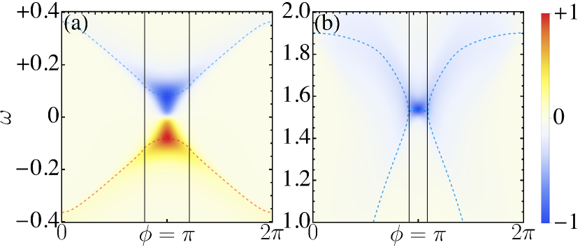
Figure 4: Normalized imaginary part of current susceptibility $\Pi(\phi,\omega)$ of NH systems. (a) $\mathrm{Im}\,\Pi(\phi,\omega)$ for the SNS junction, incorporating negative $\omega$ to reflect the particle-hole symmetry. (b) $\mathrm{Im}\,\Pi(\phi,\omega)$ for the normal mesoscopic ring. Peaks of $\mathrm{Im}\,\Pi(\phi,\omega)$ correspond to energy level transitions (dashed lines) and are concentrated between two EPs (black lines). The parameters are the same as in Fig. 1.

Conclusions and outlook.—In this work, we identified an effective distribution that captures the quantum many-body observables of NH fermionic systems in equilibrium. This distribution, derived microscopically from the biorthogonal Green’s function, serves as an extension of the Fermi-Dirac distribution for NH systems. We utilized this formalism in the context of quantum transport and derived an analytical equation for the persistent current flowing in SNS junctions and normal mesoscopic rings connected to reservoirs. We demonstrated that there are no anomalies in the persistent currents near EPs, showing that their amplitudes are suppressed by thermal fluctuations and many-body interactions. Our findings have been validated through exact diagonalization with excellent agreement. We conclude that the signatures of EPs are only discernible in a dynamical quantity—the current susceptibility—rather than a static observable.

Our formalism extends beyond quantum persistent current transport and holds promise for broader applications. It can be adapted to systems such as multi-Josephson junctions [75, 76, 77] and quantum spin chains [78], potentially unveiling new insights into their topological and entanglement characteristics. Furthermore, generalizing this formalism to encompass non-equilibrium scenarios, such as quantum pumps [79, 80, 81], shows great potential.

We acknowledge helpful discussions with D.-L. Deng, W. Brzezicki, H.-R. Wang, W.-T. Xue, L.-W. Yu, S.-Y. Zhang, and Z.-D. Liu. This work is supported by the Foundation for Polish Science through the international research agendas program co-financed by the European Union within the smart growth operational program and by the National Science Centre (Poland) OPUS Grant No. 2021/41/B/ST3/04475. P.-X.S and Z.L. acknowledge support from the Tsinghua University Dushi Program and Shanghai Qi Zhi Institute. J.L.L. acknowledges the computational resources provided by the Aalto Science-IT project.

Supplemental Material for “Non-Hermitian Persistent Current Transport”

In this Supplemental Material, we cover: ($i$) fundamental concepts of Green’s function and self-energy; ($ii$) a detailed analysis of the non-Hermitian Fermi-Dirac distribution, including gauge invariance, asymptotic behaviors, and current differentiability near EPs; ($iii$) methods for calculating the current susceptibility using non-Hermitian approaches and exact diagonalization; and ($iv$) extended numerical verifications, containing low-energy spectra and persistent currents, alongside performance benchmarks across both weak and strong coupling regimes.

I Effective Hamiltonian derivation

The self-energy for normal metals has been pedagogically introduced in Ref. [31]. Here, we outline the main procedures for incorporating the self-energy into the BdG Hamiltonian and obtain the effective Hamiltonian of superconducting systems.

I.1 Bare Green’s function of a fermionic reservoir

The tight-binding Hamiltonian of the $N_{\textsc{e}}$-site 1D fermionic wire with open boundary conditions is given by:

$$H_{\rm res} =\sum_{j=1}^{N_{\textsc{e}}}\big{(}tc^{\dagger}_{j}c_{j+1}+tc^{\dagger}_{j+1}c_{j}+gc^{\dagger}_{j}c_{j}\big{)}=\vec{C}^{\dagger}\mathcal{H}_{\rm res}\vec{C}\,,\quad\text{with}\quad\mathcal{H}_{\rm res}=\sum_{j=1}^{N_{\textsc{e}}}\big{(}t\ket{j}\bra{j+1}+t\ket{j+1}\bra{j}+g\ket{j}\bra{j}\big{)}\,.$$ (S1)

Its exact single-particle eigenvalues and normalized eigenstates are as follows:

$$\epsilon_{k}=2t\cos(k)+g\,,\quad\braket{j}{\psi_{k}}=\psi_{kj}=\sqrt{2/(N_{\textsc{e}}+1)}\sin(kj)\,,\quad k\in\{n\pi/(N_{\textsc{e}}+1)\}_{n=1}^{N_{\textsc{e}}}\,.$$ (S2)

With these quantities, we can calculate its bare Green’s function $g_{\rm res}=1/(\omega-\mathcal{H}_{\rm res})$ in the thermodynamic limit $N_{\textsc{e}}\rightarrow\infty$,

$$g_{\rm res}(l,m;\omega)=\sum_{k}\frac{\braket{l}{\psi_{k}}\braket{\psi_{k}}{m}}{\omega-\epsilon_{k}}=\frac{1}{\pi}\sum_{k}\frac{\pi}{N_{\textsc{e}}+1}\frac{\sqrt{2}\sin(kl)\sqrt{2}\sin(km)}{\omega-\epsilon_{k}}=\frac{1}{\pi}\int_{0}^{\pi}\mathrm{d}k\frac{2\sin(kl)\sin(km)}{\omega-[2t\cos(k)+g]}$$

$$=\frac{1}{2\pi}\int_{-\pi}^{\pi}\mathrm{d}k\frac{\mathrm{e}^{+\mathrm{i}k|l-m|}-\mathrm{e}^{+\mathrm{i}k|l+m|}}{\omega-[2t\cos(k)+g]}=\begin{cases}\displaystyle\frac{(-x-\sqrt{x^{2}-1})^{|l-m|}-(-x-\sqrt{x^{2}-1})^{|l+m|}}{+2t\sqrt{x^{2}-1}}\,,\quad x=\frac{g-\omega}{2t}<-1\,.\\ \displaystyle\frac{(-x+\sqrt{x^{2}-1})^{|l-m|}-(-x+\sqrt{x^{2}-1})^{|l+m|}}{-2t\sqrt{x^{2}-1}}\,,\quad x=\frac{g-\omega}{2t}>+1\,.\end{cases}$$ (S3)

When $\omega$ lies within the bandwidth $-1\leqslant x\leqslant 1$, we define the retarded ($+$) and advanced ($-$) Green’s function:

$$g_{\rm res}^{\pm}(l,m;\omega) =\frac{(-x\pm\mathrm{i}\sqrt{1-x^{2}})^{|l-m|}-(-x\pm\mathrm{i}\sqrt{1-x^{2}})^{|l+m|}}{\pm 2\mathrm{i}|t|\sqrt{1-x^{2}}}=\frac{\mathrm{e}^{\pm\mathrm{i}k|l-m|}-\mathrm{e}^{\pm\mathrm{i}k|l+m|}}{\pm 2\mathrm{i}|t|\sin(k)}\,,$$ (S4)

where we use $t<0$, $x=-\cos(k)$ and $-x\pm\mathrm{i}\sqrt{1-x^{2}}=\mathrm{e}^{\pm\mathrm{i}k}$. Next, we focus on the edge Green’s function $l=m=1$,

$$g_{\mathrm{edge}}^{\pm}(\omega)\equiv g_{\rm res}^{\pm}(1,1;\omega) =\mathrm{e}^{\pm\mathrm{i}k}/t=\big{[}(\omega-g)/2\mp\mathrm{i}\sqrt{t^{2}-[(\omega-g)/2]^{2}}\big{]}/t^{2}\,,$$ (S5)

which plays a crucial role in determining the self-energy of the reservoir connected to the system through a point contact.

I.2 Self-energy induced by a fermionic reservoir

Here we derive the self-energy for the $N$-site superconducting system, arising from its interaction with the normal reservoir. To ease the discussion, we assume that the reservoir is coupled to the right end of the system via $H_{\rm tun}=\kappa(c^{\dagger}_{\textsc{n}}c_{\textsc{n+1}}+c^{\dagger}_{\textsc{n+1}}c_{\textsc{n}})$, and rewrite the Hamiltonian of the full system $H_{\rm tot}=\vec{C}^{\dagger}\mathcal{H}_{\rm tot}\vec{C}/2$ in the basis $\vec{C}=(c_{1},c^{\dagger}_{1},\dots,c_{\textsc{n}},c^{\dagger}_{\textsc{n}},c_{\textsc{n+1}},c^{\dagger}_{\textsc{n+1}},\dots,c_{\textsc{n+n${}_{\textsc{e}}$}},c^{\dagger}_{\textsc{n+n${}_{\textsc{e}}$}})^{\textsc{t}}$ with the first-quantized Hamiltonian $\mathcal{H}_{\rm tot}=\mathcal{H}_{\rm sys}+\tilde{\mathcal{H}}_{\rm res}+\tilde{\mathcal{H}}_{\rm tun}$. We denote the extended BdG Hamiltonian with a tilde, e.g., $\tilde{\mathcal{H}}_{\rm res}=\mathcal{H}_{\rm res}\otimes\tau_{z}$ is a $2N_{\textsc{e}}\times 2N_{\textsc{e}}$ matrix as an extension of Eq. (S1) with the index $j$ running from $N+1$ to $N+N_{\textsc{e}}$, where $\tau_{z}$ is the Pauli-$Z$ matrix acting in the particle-hole space and

$$\tilde{\mathcal{H}}_{\rm tun}=\mathcal{H}_{\rm tun}\otimes\tau_{z}=\big{(}\kappa\ket{N}\bra{N+1}+\kappa\ket{N+1}\bra{N}\big{)}\otimes\tau_{z}=\begin{bmatrix}0&\mathcal{V}\\ \mathcal{V}^{\dagger}&0\end{bmatrix}\,,\quad\mathcal{V}=\begin{bmatrix}0&\cdots&0\\ \vdots&\ddots&\vdots\\ \kappa&\cdots&0\end{bmatrix}\otimes\tau_{z}\,.$$ (S6)

Given the bare Green’s function of the system $g_{\rm sys}=1/(\omega-\mathcal{H}_{\rm sys})$ and the bare Green’s function of the BdG-extended reservoir $\tilde{g}_{\rm res}=1/(\omega-\tilde{\mathcal{H}}_{\rm res})$, we compute the Green’s function $G_{\rm tot}$ of the full system by Dyson equation,

$$G_{\rm tot}=g_{\rm tot}+g_{\rm tot}\tilde{\mathcal{H}}_{\rm tun}G_{\rm tot}\quad\Longleftrightarrow\quad\begin{bmatrix}G_{\rm sys}&G_{12}\\ G_{21}&G_{\rm res}\end{bmatrix}=\begin{bmatrix}g_{\rm sys}&0\\ 0&\tilde{g}_{\rm res}\end{bmatrix}+\begin{bmatrix}g_{\rm sys}&0\\ 0&\tilde{g}_{\rm res}\end{bmatrix}\begin{bmatrix}0&\mathcal{V}\\ \mathcal{V}^{\dagger}&0\end{bmatrix}\begin{bmatrix}G_{\rm sys}&G_{12}\\ G_{21}&G_{\rm res}\end{bmatrix}\,.$$ (S7)

By eliminating $G_{12}$ and $G_{21}$, we have $G_{\rm sys}=g_{\rm sys}+g_{\rm sys}(\mathcal{V}\tilde{g}_{\rm res}\mathcal{V}^{\dagger})G_{\rm sys}\equiv g_{\rm sys}+g_{\rm sys}\Sigma(\omega)G_{\rm sys}$ and thus obtain

$$G_{\rm sys}(\omega)=\frac{1}{1/g_{\rm sys}-\Sigma(\omega)}=\frac{1}{\omega-[\mathcal{H}_{\rm sys}+\Sigma(\omega)]}\equiv\frac{1}{\omega-\mathcal{H}_{\rm eff}(\omega)}\,.$$ (S8)

To obtain the explicit form of the self-energy $\Sigma(\omega)=\mathcal{V}\tilde{g}^{+}_{\rm res}(\omega)\mathcal{V}^{\dagger}$, it is more convenient to represent the matrices back to the basis $\vec{C}=(c_{1},\dots,c_{\textsc{n}},c_{\textsc{n+1}},\dots,c_{\textsc{n+n${}_{\textsc{e}}$}},c^{\dagger}_{1},\dots,c^{\dagger}_{\textsc{n}},c^{\dagger}_{\textsc{n+1}},\dots,c^{\dagger}_{\textsc{n+n${}_{\textsc{e}}$}})^{\textsc{t}}$, which involves exchanging the particle-hole space and the lattice space, e.g., $\tilde{\mathcal{H}}_{\rm res}=\tau_{z}\otimes\mathcal{H}_{\rm res}$. As such, we can express the retarded Green’s function of the BdG-extended reservoir with $g^{\pm}_{\rm res}$ as

$$\tilde{g}^{+}_{\rm res}(\omega)=\frac{1}{\omega+\mathrm{i}\eta-\tilde{\mathcal{H}}_{\rm res}}=\begin{bmatrix}\displaystyle+1/(+\omega+\mathrm{i}\eta-\mathcal{H}_{\rm res})&0\\ 0&-1/(-\omega-\mathrm{i}\eta-\mathcal{H}_{\rm res})\end{bmatrix}=\begin{bmatrix}+g^{+}_{\rm res}(+\omega)&0\\ 0&-g^{-}_{\rm res}(-\omega)\end{bmatrix}\,,$$ (S9)

where $\eta$ is a positive infinitesimal linewidth. Using Eqs. (S5) and (S6), the self-energy is given by

$$\Sigma(\omega) =\kappa^{2}\begin{bmatrix}+g^{+}_{\mathrm{edge}}(+\omega)&0\\ 0&-g^{-}_{\mathrm{edge}}(-\omega)\end{bmatrix}\otimes\ket{N}\bra{N}=\frac{\kappa^{2}}{t^{2}}\left[\frac{\omega-g\tau_{z}}{2}-\mathrm{i}\sqrt{t^{2}-\left(\frac{\omega-g\tau_{z}}{2}\right)^{2}}\right]\otimes\ket{N}\bra{N}\,.$$ (S10)

The expression above represents the self-energy for the right-edge coupling. By replacing the lattice index $N$ with $l$ in Eq. (S10), one can similarly derive the self-energy $\Sigma_{l}(\omega)$ for a system whose $l$-site is connected to the reservoir. The self-energy $\Sigma(\omega)$ takes care of the couplings and contains all essential information about the external reservoir. Hence, as shown in Eq. (S8), $\mathcal{H}_{\rm eff}(\omega)=\mathcal{H}_{\rm sys}+\Sigma(\omega)$ effectively governs the dynamics of the system coupled to the reservoir. So far, we have not made any approximation except for $N_{\textsc{e}}\rightarrow\infty$. Since we are interested in the low-energy sector, we adopt the wide-band limit $\Sigma(\omega)\approx\Sigma(0)$ and interpret $\mathcal{H}_{\rm eff}\equiv\mathcal{H}_{\rm eff}(0)$ as an effective Hamiltonian for the system [32]. To this end, the self-energy for the superconducting system is $\Sigma_{l}(0)=-\kappa^{2}/t^{2}(\tau_{z}g/2+\mathrm{i}\sqrt{t^{2}-(g/2)^{2}})\otimes\ket{l}\bra{l}$, which also applies to normal metallic systems when $\tau_{z}$ is removed. The effective Hamiltonian of the superconducting system possesses a particle-hole symmetry $\mathcal{H}_{\rm eff}=-\tau_{x}\mathcal{H}^{*}_{\rm eff}\tau_{x}$, which is inherited from the self-energy $\Sigma(0)=-\tau_{x}\Sigma^{*}(0)\tau_{x}$, where $\tau_{x}$ is the Pauli-$X$ acting in the particle-hole space. This symmetry ensures that its complex spectra consist of pairs $(+\varepsilon_{n},-\varepsilon^{*}_{n})$, as illustrated in Fig. 1(c) and Fig. S6-4(a).

II Non-Hermitian Fermi-Dirac distribution

II.1 Derivation

To compute the correlator $\braket{c^{\dagger}_{i}c_{j}}=\int\braket{j}{\rho(\omega)}{i}f_{\textsc{fd}}(\omega)\mathrm{d}\omega$, the conventional way is to decompose $\rho(\omega)$ into two parts:

$$\rho(\omega) =\frac{\rm i}{2\pi}\sum_{n}\left[\frac{\ket{\psi^{\textsc{r}}_{n}}\bra{\psi^{\textsc{l}}_{n}}}{\omega-\varepsilon_{n}}-\frac{\ket{\psi^{\textsc{l}}_{n}}\bra{\psi^{\textsc{r}}_{n}}}{\omega-\varepsilon_{n}^{*}}\right]=\frac{\rm i}{2\pi}\sum_{n}\left[\frac{\ket{\psi^{\textsc{r}}_{n}}\bra{\psi^{\textsc{l}}_{n}}}{\omega-(\mathrm{Re}\,\varepsilon_{n}+\mathrm{i}\,\mathrm{Im}\,\varepsilon_{n})}-\frac{\ket{\psi^{\textsc{l}}_{n}}\bra{\psi^{\textsc{r}}_{n}}}{\omega-(\mathrm{Re}\,\varepsilon_{n}-\mathrm{i}\,\mathrm{Im}\,\varepsilon_{n})}\right]$$ (S11)

$$=\frac{\rm i}{2\pi}\sum_{n}\left[(\ket{\psi^{\textsc{r}}_{n}}\bra{\psi^{\textsc{l}}_{n}}-\ket{\psi^{\textsc{l}}_{n}}\bra{\psi^{\textsc{r}}_{n}})\frac{(\omega-\mathrm{Re}\,\varepsilon_{n})}{(\omega-\mathrm{Re}\,\varepsilon_{n})^{2}+(\mathrm{Im}\,\varepsilon_{n})^{2}}+(\ket{\psi^{\textsc{r}}_{n}}\bra{\psi^{\textsc{l}}_{n}}+\ket{\psi^{\textsc{l}}_{n}}\bra{\psi^{\textsc{r}}_{n}})\frac{\mathrm{i}\,\mathrm{Im}\,\varepsilon_{n}}{(\omega-\mathrm{Re}\,\varepsilon_{n})^{2}+(\mathrm{Im}\,\varepsilon_{n})^{2}}\right]\,.$$

In the context of a Hermitian system where $\mathrm{Im}\,\varepsilon_{n}\rightarrow 0$, the first part contributes to a principal value (PV) while the second part becomes a Lorentzian. In the weak coupling limit $\ket{\psi^{\textsc{l}}_{n}}\approx\ket{\psi^{\textsc{r}}_{n}}$, the PV term is close to zero and thus is often omitted in the literature [40]. However, we have found that this term is crucial for correctly evaluating observables at EPs, which are typically encountered in the strong-coupling regime. As such, we choose to calculate the correlator by analyzing the branch cut of $\ln(\varepsilon)$ along the negative real axis. Before delving into the technical details, we first introduce the following useful identities:

$$\lim_{\eta\rightarrow 0}\ln(\epsilon\pm\mathrm{i}\eta)=\ln|\epsilon|\pm\mathrm{i}\pi\Theta(-\epsilon)\,,\quad\lim_{\omega\rightarrow-\infty}\ln(\omega+\varepsilon_{n})=\mathfrak{C}+\mathrm{i}\pi\,\mathrm{sgn}(\mathrm{Im}\,\varepsilon_{n})\,,\quad\sum_{n}\big{(}\psi^{\textsc{l*}}_{ni}\psi^{\textsc{r}}_{nj}\mathfrak{C}\big{)}=\delta_{ij}\mathfrak{C}\,,$$ (S12)

where $\varepsilon_{n}\in\mathbb{C}$, $\epsilon\in\mathbb{R}$, $\eta>0$, and $\mathfrak{C}$ represents any $\varepsilon_{n}$-independent constant. This includes the scenario where $\mathfrak{C}$ grows logarithmically towards infinity, rendering any initial dependence on $\varepsilon_{n}$ negligible in that limit. Consequently, we obtain

$$\braket{c^{\dagger}_{i}c_{j}} =\frac{\rm i}{2\pi}\int_{-\infty}^{0}\sum_{n}\left(\frac{\psi^{\textsc{l*}}_{ni}\psi^{\textsc{r}}_{nj}}{\omega-\varepsilon_{n}}-\frac{\psi^{\textsc{r*}}_{ni}\psi^{\textsc{l}}_{nj}}{\omega-\varepsilon_{n}^{*}}\right)\mathrm{d}\omega=\frac{\mathrm{i}}{2\pi}\sum_{n}\left[\psi^{\textsc{l*}}_{ni}\psi^{\textsc{r}}_{nj}\ln(\omega-\varepsilon_{n})-\psi^{\textsc{r*}}_{ni}\psi^{\textsc{l}}_{nj}\ln(\omega-\varepsilon^{*}_{n})\right]\big{|}_{-\infty}^{0}$$

$$=\frac{\mathrm{i}}{2\pi}\sum_{n}\left[\psi^{\textsc{l*}}_{ni}\psi^{\textsc{r}}_{nj}\Big{(}\ln(-\varepsilon_{n})-(\mathfrak{C}+\mathrm{i}\pi)\Big{)}-\psi^{\textsc{r*}}_{ni}\psi^{\textsc{l}}_{nj}\Big{(}\ln(-\varepsilon^{*}_{n})-(\mathfrak{C}-\mathrm{i}\pi)\Big{)}\right]$$

$$=\frac{\mathrm{i}}{2\pi}\sum_{n}\left[\psi^{\textsc{l*}}_{ni}\psi^{\textsc{r}}_{nj}\Big{(}\ln|\varepsilon_{n}|+\mathrm{i}(\arg\varepsilon_{n}+\pi)-(+\mathrm{i}\pi)\Big{)}-\psi^{\textsc{r*}}_{ni}\psi^{\textsc{l}}_{nj}\Big{(}\ln|\varepsilon_{n}|-\mathrm{i}(\arg\varepsilon_{n}+\pi)-(-\mathrm{i}\pi)\Big{)}\right]$$

$$=\frac{\mathrm{i}}{2\pi}\sum_{n}\left(\psi^{\textsc{l*}}_{ni}\psi^{\textsc{r}}_{nj}\ln\varepsilon_{n}-\psi^{\textsc{r*}}_{ni}\psi^{\textsc{l}}_{nj}\ln\varepsilon_{n}^{*}\right)\equiv\frac{1}{2\mathrm{i}}\sum_{n}\left[\psi^{\textsc{l*}}_{ni}\psi^{\textsc{r}}_{nj}f_{\rm eff}(\varepsilon_{n})-\psi^{\textsc{r*}}_{ni}\psi^{\textsc{l}}_{nj}f^{*}_{\rm eff}(\varepsilon_{n})\right]\,,$$ (S13)

where we use the identities in Eq. (S12) to cancel out $\mathfrak{C}$. For $T\neq 0$, we can perform the integrals using the residue theorem:

$$\braket{c^{\dagger}_{i}c_{j}} =\frac{\rm i}{2\pi}\int_{-\infty}^{\infty}\frac{1}{\mathrm{e}^{\beta\omega}+1}\sum_{n}\left(\frac{\psi^{\textsc{l*}}_{ni}\psi^{\textsc{r}}_{nj}}{\omega-\varepsilon_{n}}-\frac{\psi^{\textsc{r*}}_{ni}\psi^{\textsc{l}}_{nj}}{\omega-\varepsilon_{n}^{*}}\right)\mathrm{d}\omega$$

$$=\frac{\mathrm{i}}{2\pi}\sum_{n}\Bigg{\{}\psi^{\textsc{l*}}_{ni}\psi^{\textsc{r}}_{nj}\frac{1}{2}\left[\frac{-2\pi\mathrm{i}}{\mathrm{e}^{\beta\varepsilon_{n}}+1}-\sum^{\infty}_{m=1}\left(m-\frac{1}{2}+\frac{\mathrm{i}\beta\varepsilon_{n}}{2\pi}\right)^{-1}-\sum^{\infty}_{m=1}\left(m-\frac{1}{2}-\frac{\mathrm{i}\beta\varepsilon_{n}}{2\pi}\right)^{-1}\right]$$

$$\qquad\quad\;\;\;\,-\psi^{\textsc{r*}}_{ni}\psi^{\textsc{l}}_{nj}\frac{1}{2}\left[\frac{+2\pi\mathrm{i}}{\mathrm{e}^{\beta\varepsilon_{n}^{*}}+1}-\sum^{\infty}_{m=1}\left(m-\frac{1}{2}+\frac{\mathrm{i}\beta\varepsilon_{n}^{*}}{2\pi}\right)^{-1}-\sum^{\infty}_{m=1}\left(m-\frac{1}{2}-\frac{\mathrm{i}\beta\varepsilon^{*}_{n}}{2\pi}\right)^{-1}\right]\Bigg{\}}$$

$$=\frac{\mathrm{i}}{2\pi}\sum_{n}\left\{\psi^{\textsc{l*}}_{ni}\psi^{\textsc{r}}_{nj}\left[\Psi\left(\frac{1}{2}+\frac{\mathrm{i}\beta\varepsilon_{n}}{2\pi}\right)-\frac{\mathrm{i}\pi}{2}\right]-\psi^{\textsc{r*}}_{ni}\psi^{\textsc{l}}_{nj}\left[\Psi\left(\frac{1}{2}+\frac{\mathrm{i}\beta\varepsilon_{n}}{2\pi}\right)-\frac{\mathrm{i}\pi}{2}\right]^{*}\right\}$$

$$\equiv\frac{1}{2\mathrm{i}}\sum_{n}\left[\psi^{\textsc{l*}}_{ni}\psi^{\textsc{r}}_{nj}f_{\rm eff}(\varepsilon_{n},\beta)-\psi^{\textsc{r*}}_{ni}\psi^{\textsc{l}}_{nj}f^{*}_{\rm eff}(\varepsilon_{n},\beta)\right]\,.$$ (S14)

Above, we use the following identities to simplify the sum of residue at $\{(m-1/2)2\pi\mathrm{i}/\beta\}_{m\in\mathbb{Z}}$ to the digamma function [67]:

$$\sum^{M}_{m=1}\frac{1}{m+z-1}=\Psi(M+z)-\Psi(z)\,,\,z\in\mathbb{C}\, \quad\Longrightarrow\quad\sum^{\infty}_{m=1}\left(m-\frac{1}{2}\pm\frac{\mathrm{i}\beta\varepsilon}{2\pi}\right)^{-1}=\mathfrak{C}-\Psi\left(\frac{1}{2}\pm\frac{\mathrm{i}\beta\varepsilon}{2\pi}\right)\,,$$

$$\Psi(1-z)-\Psi(z)=\pi\cot(\pi z)\,,\,z\in\mathbb{C}\, \quad\Longrightarrow\quad\Psi\left(\frac{1}{2}-\frac{\mathrm{i}\beta\varepsilon}{2\pi}\right)-\Psi\left(\frac{1}{2}+\frac{\mathrm{i}\beta\varepsilon}{2\pi}\right)=\frac{\pi\mathrm{i}}{\mathrm{e}^{+\beta\varepsilon}+1}-\frac{\pi\mathrm{i}}{\mathrm{e}^{-\beta\varepsilon}+1}\,,$$ (S15)

and utilize identities in Eq. (S12) to eliminate $\mathfrak{C}$ and finally obtain Eq. (II.1) with the NH Fermi-Dirac distribution $f_{\rm eff}(\varepsilon,\beta)$. It is evident that the biorthogonality of the wavefunctions is essential to cancel out the divergence in the integral. The anomalous correlator $\braket{c_{i}c_{j}}=\int\braket{j}{\rho(\omega)}{N+i}f_{\textsc{fd}}(\omega)\mathrm{d}\omega$ can be obtained similarly by replacing $i$ with $N+i$ in Eqs. (II.1)-(II.1). Therefore, a general quadratic Hermitian operator $O=\vec{C}^{\dagger}\mathcal{O}\vec{C}/\mathbf{2}$ can be computed by

$$\braket{O}=\frac{1}{2\mathrm{i}}\sum_{n}\left[\frac{\braket{\psi^{\textsc{l}}_{n}}{\mathcal{O}}{\psi^{\textsc{r}}_{n}}}{\mathbf{2}}f_{\rm eff}(\varepsilon_{n})-\frac{\braket{\psi^{\textsc{r}}_{n}}{\mathcal{O}}{\psi^{\textsc{l}}_{n}}}{\mathbf{2}}f^{*}_{\rm eff}(\varepsilon_{n})\right]=\mathrm{Im}\sum_{n}\frac{\braket{\psi^{\textsc{l}}_{n}}{\mathcal{O}}{\psi^{\textsc{r}}_{n}}}{\mathbf{2}}f_{\rm eff}(\varepsilon_{n})=\frac{\mathrm{Im}\mathrm{Tr}[\mathcal{O}f_{\rm eff}(\mathcal{H}_{\rm eff})]}{\mathbf{2}}\,,$$ (S16)

while other non-quadratic operators can be calculated using Wick’s theorem.

II.2 Gauge invariance

To examine the gauge invariance of the NH Fermi-Dirac distribution $f_{\rm eff}$, we start with a Lemma for the correlators in Eqs. (II.1)-(II.1):

Lemma 1.

Given two $\varepsilon_{n}$-independent complex numbers $C_{1}$ and $C_{2}$, applying two separate transformations on the NH Fermi-Dirac distribution $f_{\rm eff}\rightarrow f_{\rm eff}+C_{1}$ and its conjugate $f^{*}_{\rm eff}\rightarrow[f_{\rm eff}+C_{2}]^{*}$ will keep $\braket{c_{i}c_{j}}$ unchanged while transforming

$$\braket{c^{\dagger}_{i}c_{j}}\rightarrow\braket{c^{\dagger}_{i}c_{j}}+\frac{1}{2\mathrm{i}}\delta_{ij}(C_{1}-C^{*}_{2})\,.$$ (S17)

This Lemma naturally follows from the biorthogonality of wavefunctions in Eq. (S12) and contributes the following theorem:

Theorem 1.

Observables are invariant under the gauge transformation on the NH Fermi-Dirac distribution $f_{\rm eff}\rightarrow f_{\rm eff}+\mathbb{R}$.

Proof.

According to Eq. (S17) in Lemma 1, the correlator $\braket{c^{\dagger}_{i}c_{j}}$ remains unchanged when $C_{1}=C^{*}_{2}$. In general, $C_{1}$ is not required to be equal to $C_{2}$. However, this results in two NH Fermi-Dirac distributions $f_{\rm eff}+C_{1}$ and $f_{\rm eff}+C_{2}$ within a single correlator. Hence, we set $C_{1}=C_{2}=C$ and find $\braket{c^{\dagger}_{i}c_{j}}\rightarrow\braket{c^{\dagger}_{i}c_{j}}+\delta_{ij}\mathrm{Im}(C)$, which directly leads to

$$\braket{O}\rightarrow\braket{O}+\mathrm{Tr}(\mathcal{O})\,\mathrm{Im}(C)\,.$$ (S18)

Therefore, the observable computed by a general quadratic Hermitian operator in Eq. (5) is gauge-invariant when $C\in\mathbb{R}$. ∎

Corollary 1.

Observables associated with traceless operators are invariant under gauge transformations of two NH Fermi-Dirac distributions $f_{\rm eff}\rightarrow f_{\rm eff}+C_{1}$ and $f^{*}_{\rm eff}\rightarrow[f_{\rm eff}+C_{2}]^{*}$, where $C_{1}$ and $C_{2}$ are two $\varepsilon_{n}$-independent complex numbers.

This Corollary can be readily derived from Eq. (S17) in Lemma 1 and Eq. (S18) in Theorem 1. An paradigmatic instance for a traceless operator is the persistent current operator $\mathcal{J}$ studied in this work. To obtain the analytical expression in Eq. (1) at zero temperature, we transform $f_{\rm eff}$ by assigning specific values to $C_{1}$ and $C_{2}$:

$$I(\phi) =\frac{\mathrm{i}}{2\pi}\sum_{n}\left(\frac{\mathrm{d}\varepsilon_{n}}{\mathrm{d}\phi}\ln\varepsilon_{n}-\frac{\mathrm{d}\varepsilon^{*}_{n}}{\mathrm{d}\phi}\ln\varepsilon^{*}_{n}\right)=\frac{\mathrm{i}}{2\pi}\sum_{n}\left[\frac{\mathrm{d}\varepsilon_{n}}{\mathrm{d}\phi}(\ln\varepsilon_{n}+1)-\frac{\mathrm{d}\varepsilon^{*}_{n}}{\mathrm{d}\phi}(\ln\varepsilon^{*}_{n}+1)\right],\quad\text{with}\quad C_{1}=C_{2}=-\frac{1}{\pi}\,,$$

$$=\frac{\mathrm{i}}{2\pi}\frac{\mathrm{d}}{\mathrm{d}\phi}\sum_{n}\left(\varepsilon_{n}\ln\varepsilon_{n}-\varepsilon^{*}_{n}\ln\varepsilon^{*}_{n}\right)=-\frac{1}{\pi}\frac{\mathrm{d}}{\mathrm{d}\phi}\mathrm{Im}\sum_{n}\varepsilon_{n}\ln\varepsilon_{n}=-\frac{1}{\pi}\frac{\mathrm{d}}{\mathrm{d}\phi}\mathrm{Im}\mathrm{Tr}\left(\mathcal{H}_{\rm eff}\ln\mathcal{H}_{\rm eff}\right)\,.$$ (S19)

One can proceed to transform with $C_{1}=0,\;C_{2}=+\mathrm{i}$ and exploit the particle-hole symmetry of superconductors, $\varepsilon_{-n}=-\varepsilon^{*}_{n}$, to obtain $\mathrm{i}/\pi\,\partial_{\phi}\mathrm{Tr}(\mathcal{H}_{\rm eff}\ln\mathcal{H}_{\rm eff})$ that is specific for supercurrents. In the same vein, the persistent current at $T\neq 0$ is given by

$$I(\phi) =\frac{\mathrm{i}}{2\pi}\sum_{n}\left\{\frac{\mathrm{d}\varepsilon_{n}}{\mathrm{d}\phi}\left[\Psi\left(\frac{1}{2}+\frac{\mathrm{i}\beta\varepsilon_{n}}{2\pi}\right)-\frac{\mathrm{i}\pi}{2}\right]-\frac{\mathrm{d}\varepsilon^{*}_{n}}{\mathrm{d}\phi}\left[\Psi\left(\frac{1}{2}+\frac{\mathrm{i}\beta\varepsilon_{n}}{2\pi}\right)-\frac{\mathrm{i}\pi}{2}\right]^{*}\right\}\,,\qquad\qquad\;\text{with}\quad C_{1}=C_{2}=-\frac{\mathrm{i}}{2}\,,$$

$$=\frac{\mathrm{i}}{2\pi}\sum_{n}\left[\frac{\mathrm{d}\varepsilon_{n}}{\mathrm{d}\phi}\Psi\left(\frac{1}{2}+\frac{\mathrm{i}\beta\varepsilon_{n}}{2\pi}\right)-\frac{\mathrm{d}\varepsilon^{*}_{n}}{\mathrm{d}\phi}\Psi\left(\frac{1}{2}-\frac{\mathrm{i}\beta\varepsilon^{*}_{n}}{2\pi}\right)\right]=\frac{1}{\beta}\frac{\mathrm{d}}{\mathrm{d}\phi}\sum_{n}\left[\mathrm{log\Gamma}\left(\frac{1}{2}+\frac{\mathrm{i}\beta\varepsilon_{n}}{2\pi}\right)+\mathrm{log\Gamma}\left(\frac{1}{2}+\frac{\mathrm{i}\beta\varepsilon_{n}}{2\pi}\right)^{*}\right]$$

$$=\frac{2}{\beta}\frac{\mathrm{d}}{\mathrm{d}\phi}\sum_{n}\mathrm{Re}\,\mathrm{log\Gamma}\left(\frac{1}{2}+\frac{\mathrm{i}\beta\varepsilon_{n}}{2\pi}\right)=\frac{2}{\beta}\frac{\mathrm{d}}{\mathrm{d}\phi}\mathrm{Re}\,\mathrm{Tr}\,\mathrm{log\Gamma}\left(\frac{1}{2}+\frac{\mathrm{i}\beta}{2\pi}\mathcal{H}_{\rm eff}\right)\,.$$ (S20)

Similarly, the particle-hole symmetry of superconductors implies $\varepsilon_{-n}=-\varepsilon^{*}_{n}$, which in turn can be used to eliminate the $\mathrm{Re}$ operation for supercurrents.

II.3 Asymptotic behavior

We denote $\epsilon=\mathrm{Re}\,\varepsilon$ and summarize the asymptotic behavior of $f_{\rm eff}$ in the Hermitian limit where $\mathrm{Im}\,\varepsilon\rightarrow 0$,

$$f_{\rm eff}(\varepsilon)=\begin{cases}\displaystyle-\frac{1}{\pi}\ln|\epsilon|+\mathrm{i}\Theta(-\epsilon)\,,&T=0\\ \displaystyle-\frac{1}{\pi}\mathrm{Re}\left[\Psi\left(\frac{1}{2}+\frac{\mathrm{i}\beta\epsilon}{2\pi}\right)\right]+\mathrm{i}\frac{1}{\mathrm{e}^{\beta\epsilon}+1}\,,&T\neq 0\\ \end{cases}\;\Longrightarrow\;\mathrm{Im}\,f_{\rm eff}(\varepsilon)=\begin{cases}\displaystyle f_{\textsc{fd}}(\epsilon)=\Theta(-\epsilon)\,,&T=0\\ \displaystyle f_{\textsc{fd}}(\epsilon,\beta)=\frac{1}{\mathrm{e}^{\beta\epsilon}+1}\,,&T\neq 0\\ \end{cases}\,,$$ (S21)

which is illustrated in Fig. 3(c). To extract the asymptotic behavior for the inverse temperature $\beta=1/k_{\textsc{b}}T$ we write:

$$f_{\rm eff}(\varepsilon,\beta)=\begin{cases}\displaystyle-\frac{1}{\pi}\left[\cancel{\ln\left(\frac{\beta}{2\pi}\right)}+\ln(\varepsilon)-\frac{\pi^{2}}{6\beta^{2}\varepsilon^{2}}\right]\cong-\frac{1}{\pi}\left(\ln\varepsilon-\frac{\pi^{2}}{6\beta^{2}\varepsilon^{2}}\right)\,,&\beta\rightarrow\infty\\ \displaystyle-\frac{1}{\pi}\left[\cancel{\Psi\left(\frac{1}{2}\right)}-\mathrm{i}\pi\Big{(}\frac{1}{2}-\frac{\beta\varepsilon}{4}\Big{)}\right]\cong\mathrm{i}\Big{(}\frac{1}{2}-\frac{\beta\varepsilon}{4}\Big{)}\,,&\beta\rightarrow 0\\ \end{cases}\,,$$ (S22)

where we use $\cong$ to represent the gauge equivalence after eliminating real constants according to Theorem 1. The first line goes back to the $T=0$ expression. The imaginary of the second line is consistent with the expansion of $f_{\textsc{fd}}(\varepsilon,\beta)$ at $\beta\rightarrow 0$. The asymptotic behavior of the persistent current $I(\phi)$ in the Hermitian limit is summarized below:

$$I(\phi)=\begin{cases}\displaystyle-\frac{1}{\pi}\frac{\mathrm{d}}{\mathrm{d}\phi}\mathrm{Im}\sum_{n}\epsilon_{n}\left[\cancel{\ln|\epsilon_{n}|}-\mathrm{i}\pi\Theta(-\epsilon_{n})\right]=\underbrace{\frac{\mathrm{d}}{\mathrm{d}\phi}\sum_{n\leqslant 0}\epsilon_{n}=\frac{\mathrm{d}E_{0}}{\mathrm{d}\phi}}_{\text{normal metal}}=\underbrace{2\frac{\mathrm{d}}{\mathrm{d}\phi}\sum_{n\leqslant 0}\frac{\epsilon_{n}}{2}=2\frac{\mathrm{d}E_{0}}{\mathrm{d}\phi}}_{\text{superconductor}}\,,&T=0\\ \displaystyle\frac{1}{\beta}\frac{\mathrm{d}}{\mathrm{d}\phi}\sum_{n}\left[\cancel{\ln(2\pi)+\frac{\beta\epsilon_{n}}{2}}-\ln(1+\mathrm{e}^{\beta\epsilon_{n}})\right]=\frac{\mathrm{d}}{\mathrm{d}\phi}\left(\frac{\ln Z}{-\beta}\right)=\frac{\mathrm{d}F}{\mathrm{d}\phi}\,,&\text{normal metal}\\ \displaystyle\frac{1}{\beta}\frac{\mathrm{d}}{\mathrm{d}\phi}\sum_{n}\left[\cancel{\ln(2\pi)}-\ln(\mathrm{e}^{+\beta\epsilon_{n}/2}+\mathrm{e}^{-\beta\epsilon_{n}/2})\right]=2\frac{\mathrm{d}}{\mathrm{d}\phi}\sum_{n\geqslant 0}\left[-\frac{1}{\beta}\ln(\mathrm{e}^{+\beta\epsilon_{n}/2}+\mathrm{e}^{-\beta\epsilon_{n}/2})\right]=2\frac{\mathrm{d}F}{\mathrm{d}\phi}\,,&\text{superconductor}\end{cases}$$

where $Z$ is the partition function, $F$ is the free energy, and we remove the crossed terms based on the fact that the trace of the Hamiltonian is independent of $\phi$. To obtain the last two lines at finite temperatures, we should utilize the reflection identity of $\mathrm{log\Gamma}$ [68] to expand the $\mathrm{Re}\mathrm{Tr}$ term in Eq. (9):

$$\mathrm{log\Gamma}(1-z)+\mathrm{log\Gamma}(z)=\ln(\pi)-\ln\sin(\pi z)\,,\quad z=\frac{1}{2}+\frac{\mathrm{i}\beta\epsilon}{2\pi}\,,\quad-\frac{1}{2}<\mathrm{Re}(z)<\frac{\pi}{2}\,,\quad\epsilon\in\mathbb{R}\,.$$ (S23)

II.4 Current differentiability near EPs

In the vicinity of a second-order EP at $\varepsilon_{\textsc{ep}}$, the eigenvalues $\varepsilon_{\pm}(\phi)$ follow a square-root scaling as a function of $\phi$:

$$\varepsilon_{\pm}(\phi)=\varepsilon_{\textsc{ep}}\pm\sqrt{s(\phi)}=\mu-\mathrm{i}\nu(\phi)\pm\sqrt{s(\phi)},\quad\varepsilon^{\prime}_{\pm}(\phi)=-\mathrm{i}\nu^{\prime}(\phi)\pm\frac{s^{\prime}(\phi)}{2\sqrt{s(\phi)}}\,,$$ (S24)

where $\nu(\phi)$ and $s(\phi)$ are bounded functions and smoothly vary as $\phi$ [21]. We use an EP-subscript to represent the value of a variable at EP. The derivatives of two EP-modes $\varepsilon^{\prime}_{\pm}(\phi_{\textsc{ep}})$ are divergent at the EP due to the function inside the square root $\lim_{\phi\rightarrow\phi_{\textsc{ep}}}s(\phi)=0$. In the following discussion on differentiability, we omit the explicit dependence on $\phi$ unless otherwise stated. We first analyze the trace term in the persistent current $I(\phi)=-1/\pi\;\partial_{\phi}\mathrm{Im}\mathrm{Tr}(\mathcal{H}_{\rm eff}\ln\mathcal{H}_{\rm eff})$ at $T=0$,

$$\mathrm{Tr}(\mathcal{H}_{\rm eff}\ln\mathcal{H}_{\rm eff}) =\sum_{n=\pm}\varepsilon_{n}\ln\varepsilon_{n}+\sum_{n\neq\pm}\varepsilon_{n}\ln\varepsilon_{n}=\frac{\varepsilon_{+}-\varepsilon_{-}}{2}(\ln\varepsilon_{+}-\ln\varepsilon_{-})+\frac{\varepsilon_{+}+\varepsilon_{-}}{2}(\ln\varepsilon_{+}+\ln\varepsilon_{-})+\sum_{n\neq\pm}\varepsilon_{n}\ln\varepsilon_{n}$$

$$=\sqrt{s(\phi)}(\ln\varepsilon_{+}-\ln\varepsilon_{-})+[\mu-\mathrm{i}\nu(\phi)](\ln\varepsilon_{+}+\ln\varepsilon_{-})+\sum_{n\neq\pm}\varepsilon_{n}\ln\varepsilon_{n}\,.$$ (S25)

The last term above is from the bulk states and is differentiable near EPs, thus we can only analyze the EP-modes $\varepsilon_{\pm}(\phi)$,

$$\frac{\mathrm{d}}{\mathrm{d}\phi}\sum_{n=\pm}\varepsilon_{n}\ln\varepsilon_{n} =\varepsilon^{\prime}_{+}(1+\ln\varepsilon_{+})+\varepsilon^{\prime}_{-}(1+\ln\varepsilon_{-})=\frac{\varepsilon^{\prime}_{+}-\varepsilon^{\prime}_{-}}{2}(\ln\varepsilon_{+}-\ln\varepsilon_{-})+\frac{\varepsilon^{\prime}_{+}+\varepsilon^{\prime}_{-}}{2}(2+\ln\varepsilon_{+}+\ln\varepsilon_{-})$$ (S26)

$$=s^{\prime}(\phi)\frac{\ln\big{(}\varepsilon_{\textsc{ep}}+\sqrt{s(\phi)}\big{)}-\ln\big{(}\varepsilon_{\textsc{ep}}-\sqrt{s(\phi)}\big{)}}{2\sqrt{s(\phi)}}-\mathrm{i}\nu^{\prime}(\phi)\left[2+\ln\big{(}\varepsilon_{\textsc{ep}}+\sqrt{s(\phi)}\big{)}+\ln\big{(}\varepsilon_{\textsc{ep}}-\sqrt{s(\phi)}\big{)}\right]\,,$$

where we substitute the square-root expansion in Eq. (S24). Using $\lim_{\phi\rightarrow\phi_{\textsc{ep}}}s(\phi)=0$, we obtain

$$\lim_{\phi\rightarrow\phi_{\textsc{ep}}}\frac{\mathrm{d}}{\mathrm{d}\phi}\sum_{n=\pm}\varepsilon_{n}\ln\varepsilon_{n} =\frac{s^{\prime}(\phi_{\textsc{ep}})}{\varepsilon_{\textsc{ep}}}-\mathrm{i}\nu^{\prime}(\phi_{\textsc{ep}})(2+2\ln\varepsilon_{\textsc{ep}})=-\pi\left[s^{\prime}(\phi_{\textsc{ep}})f^{\prime}_{\rm eff}(\varepsilon_{\textsc{ep}})-2\mathrm{i}\nu^{\prime}(\phi_{\textsc{ep}})\left(f_{\rm eff}(\varepsilon_{\textsc{ep}})-\frac{1}{\pi}\right)\right]\,.$$ (S27)

Following similar steps, we obtain the contribution of two EP-modes in the trace term at $T\neq 0$,

$$\lim_{\phi\rightarrow\phi_{\textsc{ep}}}\frac{\mathrm{d}}{\mathrm{d}\phi}\sum_{n=\pm}\mathrm{log\Gamma}\left(\frac{1}{2}+\frac{\mathrm{i}\beta\varepsilon_{n}}{2\pi}\right) =\frac{\beta}{2\mathrm{i}}\left[s^{\prime}(\phi_{\textsc{ep}})f^{\prime}_{\rm eff}(\varepsilon_{\textsc{ep}},\beta)-2\mathrm{i}\nu^{\prime}(\phi_{\textsc{ep}})\left(f_{\rm eff}(\varepsilon_{\textsc{ep}},\beta)-\frac{\mathrm{i}}{2}\right)\right]\,.$$ (S28)

Due to the analyticity of $f_{\rm eff}(\varepsilon,\beta)$ in the lower complex plane, both Eqs. (S27) and (S28) are bounded, ensuring that the persistent current $I(\phi)$ exhibits a continuous and smooth behavior in the vicinity of EPs.

III Current Susceptibility

III.1 Non-Hermitian approach

The current susceptibility in superconducting systems can be expanded into a set of four-point electronic correlators by substituting the site-resolved current operator in the Heisenberg picture $J(\tau)=-\mathrm{i}t_{j}[c^{\dagger}_{j}(\tau)c_{j+1}(\tau)-c^{\dagger}_{j+1}(\tau)c_{j}(\tau)]$:

$$\Pi(\tau)=-\mathrm{i}\Theta(\tau)\braket{[J(\tau),J(0)]}=-\mathrm{i}\Theta(\tau)(-t_{j}^{2})\braket{[c^{\dagger}_{j}(\tau)c_{j+1}(\tau)-c^{\dagger}_{j+1}(\tau)c_{j}(\tau),c^{\dagger}_{j}c_{j+1}-c^{\dagger}_{j+1}c_{j}]}$$ (S29)

$$=\mathrm{i}\Theta(\tau)t_{j}^{2}\left[\braket{[c^{\dagger}_{j}(\tau)c_{j+1}(\tau),c^{\dagger}_{j}c_{j+1}]}-\braket{[c^{\dagger}_{j}(\tau)c_{j+1}(\tau),c^{\dagger}_{j+1}c_{j}]}+\braket{[c^{\dagger}_{j+1}(\tau)c_{j}(\tau),c^{\dagger}_{j+1}c_{j}]}-\braket{[c^{\dagger}_{j+1}(\tau)c_{j}(\tau),c^{\dagger}_{j}c_{j+1}]}\right]\,,$$

where we denote $c_{j}\equiv c_{j}(0)$ and omit the subscript in $J\equiv J_{j}$, since $j$ is always set at the first site of $\mathbb{N}$. Using identities for the propagator $\mathrm{i}\tilde{g}(\tau)$ and the lesser Green’s function [41],

$$\{c_{i}(\tau),c^{\dagger}_{j}\}=\mathrm{i}\tilde{g}_{i,j}(\tau)\,,\quad\{c_{i}(\tau),c_{j}\} =\mathrm{i}\tilde{g}_{i,N+j}(\tau)\,,\quad\{c^{\dagger}_{i}(\tau),c^{\dagger}_{j}\}=\mathrm{i}\tilde{g}_{N+i,j}(\tau)\,,$$ (S30)

$$\braket{c^{\dagger}_{i}c_{j}(\tau)}=\int\mathrm{d}\omega\mathrm{e}^{-\mathrm{i}\omega\tau}f_{\textsc{fd}}(\omega)\rho_{j,i}(\omega)\,,\braket{c_{i}c_{j}(\tau)} =\int\mathrm{d}\omega\mathrm{e}^{-\mathrm{i}\omega\tau}f_{\textsc{fd}}(\omega)\rho_{j,N+i}(\omega)\,,\braket{c^{\dagger}_{i}c^{\dagger}_{j}(\tau)}=\int\mathrm{d}\omega\mathrm{e}^{-\mathrm{i}\omega\tau}f_{\textsc{fd}}(\omega)\rho_{N+j,i}(\omega)\,,$$

we can transform the four-point electronic correlator to an integral involving the density of state operator $\rho_{i,j}(\omega)\equiv\braket{i}{\rho(\omega)}{j}$,

$$\braket{[c^{\dagger}_{i}(\tau)c_{j}(\tau),c^{\dagger}_{k}c_{l}]} =\int_{-\infty}^{\infty}\mathrm{d}\omega_{1}\mathrm{d}\omega_{2}f_{\textsc{fd}}(\omega_{1})\Big{[}\rho_{j,k}(\omega_{2})\rho_{l,i}(\omega_{1})\mathrm{e}^{-\mathrm{i}(\omega_{1}-\omega_{2})(-\tau)}-\rho_{l,i}(\omega_{2})\rho_{j,k}(\omega_{1})\mathrm{e}^{-\mathrm{i}(\omega_{1}-\omega_{2})(+\tau)}$$

$$\qquad\qquad+\rho_{N+k,i}(\omega_{2})\rho_{j,N+l}(\omega_{1})\mathrm{e}^{-\mathrm{i}(\omega_{1}-\omega_{2})(+\tau)}-\rho_{j,N+l}(\omega_{2})\rho_{N+k,i}(\omega_{1})\mathrm{e}^{-\mathrm{i}(\omega_{1}-\omega_{2})(-\tau)}\Big{]}\,.$$ (S31)

Substituting Eq. (III.1) back to each four-point correlator in Eq. (S29), and then performing the Fourier transform, we get

$$\Pi(\omega)=\int\mathrm{d}\tau\Pi(\tau)\mathrm{e}^{+\mathrm{i}\omega\tau}=(-t_{j}^{2})\int_{-\infty}^{\infty}\mathrm{d}\omega_{1}\mathrm{d}\omega_{2}\frac{f_{\textsc{fd}}(\omega_{1})-f_{\textsc{fd}}(\omega_{2})}{\omega+\omega_{1}-\omega_{2}+\mathrm{i}\eta}$$ (S32)

$$\times\Big{\{}[\rho_{j+1,j}(\omega_{1})\rho_{j+1,j}(\omega_{2})-\rho_{j,j}(\omega_{1})\rho_{j+1,j+1}(\omega_{2})+\rho_{j,j+1}(\omega_{1})\rho_{j,j+1}(\omega_{2})-\rho_{j+1,j+1}(\omega_{1})\rho_{j,j}(\omega_{2})]+$$

$$[\rho_{N+j+1,j}(\omega_{1})\rho_{j+1,N+j}(\omega_{2})-\rho_{N+j,j}(\omega_{1})\rho_{j+1,N+j+1}(\omega_{2})+\rho_{N+j,j+1}(\omega_{1})\rho_{j,N+j+1}(\omega_{2})-\rho_{N+j+1,j+1}(\omega_{1})\rho_{j,N+j}(\omega_{2})]\Big{\}}\,.$$

Using the identify $\lim_{\eta\rightarrow 0^{+}}[1/(x\pm\mathrm{i}\eta)]=\mathrm{PV}\left(1/x\right)\mp\mathrm{i}\pi\delta(x)$, we obtain its imaginary part

$$\mathrm{Im}\;\Pi(\omega)=\pi t_{j}^{2}\int_{-\infty}^{\infty}\mathrm{d}\omega_{1}\mathrm{d}\omega_{2}\delta(\omega+\omega_{1}-\omega_{2})[f_{\textsc{fd}}(\omega_{1})-f_{\textsc{fd}}(\omega_{2})]$$ (S33)

$$\times\mathrm{Re}\Big{\{}[\rho_{j+1,j}(\omega_{1})\rho_{j+1,j}(\omega_{2})-\rho_{j,j}(\omega_{1})\rho_{j+1,j+1}(\omega_{2})+\rho_{j,j+1}(\omega_{1})\rho_{j,j+1}(\omega_{2})-\rho_{j+1,j+1}(\omega_{1})\rho_{j,j}(\omega_{2})]+$$

$$[\rho_{N+j+1,j}(\omega_{1})\rho_{j+1,N+j}(\omega_{2})-\rho_{N+j,j}(\omega_{1})\rho_{j+1,N+j+1}(\omega_{2})+\rho_{N+j,j+1}(\omega_{1})\rho_{j,N+j+1}(\omega_{2})-\rho_{N+j+1,j+1}(\omega_{1})\rho_{j,N+j}(\omega_{2})]\Big{\}}\,.$$

Specifically in the zero temperature $f_{\textsc{fd}}(\omega)=\Theta(-\omega)$, we can exploit the $\delta$-function to integrate out $\omega_{2}$ and thus obtain Eq. (Non-Hermitian Persistent Current Transport) in the main text. The integral $P_{ijkl}(\omega)\equiv\int_{-\infty}^{0}\braket{i}{\rho(\omega^{\prime})}{j}\braket{k}{\rho(\omega+\omega^{\prime})}{l}\mathrm{d}\omega^{\prime}$ can be analytically derived as follows:

$$P_{ijkl}(\omega)=\Big{(}\frac{\rm i}{2\pi}\Big{)}^{2}\int_{-\infty}^{0}\sum_{nm}\left[\frac{\braket{i}{\psi^{\textsc{r}}_{n}}\braket{\psi^{\textsc{l}}_{n}}{j}}{\omega^{\prime}-\varepsilon_{n}}-\frac{\braket{i}{\psi^{\textsc{l}}_{n}}\braket{\psi^{\textsc{r}}_{n}}{j}}{\omega^{\prime}-\varepsilon_{n}^{*}}\right]\left[\frac{\braket{k}{\psi^{\textsc{r}}_{m}}\braket{\psi^{\textsc{l}}_{m}}{l}}{\omega^{\prime}+\omega-\varepsilon_{m}}-\frac{\braket{k}{\psi^{\textsc{l}}_{m}}\braket{\psi^{\textsc{r}}_{m}}{l}}{\omega^{\prime}+\omega-\varepsilon_{m}^{*}}\right]\mathrm{d}\omega^{\prime}$$

$$=\Big{(}\frac{\rm i}{2\pi}\Big{)}^{2}\sum_{nm}\int_{-\infty}^{0}\left[\frac{\psi^{\textsc{r}}_{ni}\psi^{\textsc{l*}}_{nj}}{\omega^{\prime}-\varepsilon_{n}}\frac{\psi^{\textsc{r}}_{mk}\psi^{\textsc{l*}}_{ml}}{\omega^{\prime}+\omega-\varepsilon_{m}}-\frac{\psi^{\textsc{r}}_{ni}\psi^{\textsc{l*}}_{nj}}{\omega^{\prime}-\varepsilon_{n}}\frac{\psi^{\textsc{l}}_{mk}\psi^{\textsc{r*}}_{ml}}{\omega^{\prime}+\omega-\varepsilon_{m}^{*}}+\frac{\psi^{\textsc{l}}_{ni}\psi^{\textsc{r*}}_{nj}}{\omega^{\prime}-\varepsilon_{n}^{*}}\frac{\psi^{\textsc{l}}_{mk}\psi^{\textsc{r*}}_{ml}}{\omega^{\prime}+\omega-\varepsilon_{m}^{*}}-\frac{\psi^{\textsc{l}}_{ni}\psi^{\textsc{r*}}_{nj}}{\omega^{\prime}-\varepsilon_{n}^{*}}\frac{\psi^{\textsc{r}}_{mk}\psi^{\textsc{l*}}_{ml}}{\omega^{\prime}+\omega-\varepsilon_{m}}\right]\mathrm{d}\omega^{\prime}$$

$$=\Big{(}\frac{\rm i}{2\pi}\Big{)}^{2}\sum_{nm}\Big{[}+\psi^{\textsc{r}}_{ni}\psi^{\textsc{l*}}_{nj}\psi^{\textsc{r}}_{mk}\psi^{\textsc{l*}}_{ml}\frac{\ln(-\varepsilon_{n})-\ln(-\varepsilon_{m}+\omega)}{\varepsilon_{n}-\varepsilon_{m}+\omega}-\psi^{\textsc{r}}_{ni}\psi^{\textsc{l*}}_{nj}\psi^{\textsc{l}}_{mk}\psi^{\textsc{r*}}_{ml}\frac{\ln(+\varepsilon_{n})-\ln(+\varepsilon^{*}_{m}-\omega)}{\varepsilon_{n}-\varepsilon^{*}_{m}+\omega}$$

$$\qquad\qquad\qquad\;\;+\psi^{\textsc{l}}_{ni}\psi^{\textsc{r*}}_{nj}\psi^{\textsc{l}}_{mk}\psi^{\textsc{r*}}_{ml}\frac{\ln(-\varepsilon^{*}_{n})-\ln(-\varepsilon^{*}_{m}+\omega)}{\varepsilon^{*}_{n}-\varepsilon^{*}_{m}+\omega}-\psi^{\textsc{l}}_{ni}\psi^{\textsc{r*}}_{nj}\psi^{\textsc{r}}_{mk}\psi^{\textsc{l*}}_{ml}\frac{\ln(+\varepsilon^{*}_{n})-\ln(+\varepsilon_{m}-\omega)}{\varepsilon^{*}_{n}-\varepsilon_{m}+\omega}\Big{]}\,.$$ (S34)

One can simplify Eq. (III.1) into Eq. (12) by using $f_{\rm eff}(\varepsilon)=-(1/\pi)\ln\varepsilon$ and the definition of $p^{nm\pm}_{ijkl}$ in the main text.

III.2 Exact diagonalization

In the Hermitian case, the time evolution of the fermionic operator in superconducting systems can be expressed as $c_{j}(\tau)=\sum_{n}[u_{n}(j)\mathrm{e}^{-\mathrm{i}\epsilon_{n}\tau}d_{n}+v^{*}_{n}(j)\mathrm{e}^{+\mathrm{i}\epsilon_{n}\tau}d^{\dagger}_{n}]$, where it involves a set of Bogoliubons $d_{n}$ with energy $\epsilon_{n}$ and the wavefunction $\psi_{n}=[\psi_{n}(1),\dots,\psi_{n}(N),\psi_{n}(N+1),\dots,\psi_{n}(2N)]^{\textsc{t}}=[u_{n}(1),\dots,u_{n}(N),v_{n}(1),\dots,v_{n}(N)]^{\textsc{t}}$. Hence, the current operator reads

$$J(\tau) =-t_{j}\sum_{nm}\Big{[}A_{nm}\mathrm{e}^{+\mathrm{i}(\epsilon_{n}-\epsilon_{m})\tau}d^{\dagger}_{n}d_{m}+B_{nm}\mathrm{e}^{-\mathrm{i}(\epsilon_{n}+\epsilon_{m})\tau}d_{n}d_{m}+B^{*}_{mn}\mathrm{e}^{+\mathrm{i}(\epsilon_{n}+\epsilon_{m})\tau}d^{\dagger}_{n}d^{\dagger}_{m}+C_{nm}\Big{]}\,,$$

$$A_{nm} =\mathrm{i}[u^{*}_{n}(j)u_{m}(j+1)-u^{*}_{n}(j+1)u_{m}(j)]-\mathrm{i}[v_{m}(j)v^{*}_{n}(j+1)-v_{m}(j+1)v^{*}_{n}(j)]\,,$$

$$B_{nm} =\mathrm{i}[v_{n}(j)u_{m}(j+1)-v_{n}(j+1)u_{m}(j)]\,,\qquad C_{nm}=\mathrm{i}\delta_{nm}[v_{n}(j)v^{*}_{n}(j+1)-v_{n}(j+1)v^{*}_{n}(j)]\,.$$ (S35)

The current susceptibility $\Pi(\tau)$ and its Fourier transform $\Pi(\omega)$ can be calculated using the occupation of Bogoliubons $\braket{d^{\dagger}_{n}d_{m}}=\delta_{nm}f_{\textsc{fd}}(\epsilon_{n})$ (refer to Appendix D of Ref. [82] for a pedagogical derivation),

$$\Pi(\tau) =-\mathrm{i}\Theta(\tau)\braket{[J(\tau),J(0)]}=-\mathrm{i}\Theta(\tau)t_{j}^{2}\sum_{nm}\Big{\{}A_{nm}A_{mn}\mathrm{e}^{+\mathrm{i}(\epsilon_{n}-\epsilon_{m})\tau}[f_{\textsc{fd}}(\epsilon_{n})-f_{\textsc{fd}}(\epsilon_{m})]$$

$$\qquad+B_{nm}(B^{*}_{nm}-B^{*}_{mn})\mathrm{e}^{-\mathrm{i}(\epsilon_{n}+\epsilon_{m})\tau}[f(-\epsilon_{n})-f_{\textsc{fd}}(\epsilon_{m})]+B^{*}_{mn}(B_{mn}-B_{nm})\mathrm{e}^{+\mathrm{i}(\epsilon_{n}+\epsilon_{m})\tau}[f_{\textsc{fd}}(\epsilon_{n})-f(-\epsilon_{m})]\Big{\}}\,,$$

$$\Pi(\omega) =\int\mathrm{d}\tau\Pi(\tau)\mathrm{e}^{+\mathrm{i}\omega\tau}=t_{j}^{2}\sum_{nm}\bigg{[}A_{nm}A_{mn}\frac{f_{\textsc{fd}}(\epsilon_{n})-f_{\textsc{fd}}(\epsilon_{m})}{\omega+\epsilon_{n}-\epsilon_{m}+\mathrm{i}\eta}$$

$$\qquad+B_{nm}(B^{*}_{mn}-B^{*}_{nm})\frac{f_{\textsc{fd}}(\epsilon_{m})+f_{\textsc{fd}}(\epsilon_{n})-1}{\omega-\epsilon_{n}-\epsilon_{m}+\mathrm{i}\eta}+B^{*}_{mn}(B_{nm}-B_{mn})\frac{1-f_{\textsc{fd}}(\epsilon_{m})-f_{\textsc{fd}}(\epsilon_{n})}{\omega+\epsilon_{n}+\epsilon_{m}+\mathrm{i}\eta}\bigg{]}\,.$$ (S36)

We remark that Eqs. (III.2) and (III.2) still apply to normal metals by setting all the wavefunctions $v_{n}=0$. This enables us to perform an exact diagonalization of the full Hermitian system $H_{\rm tot}$ including a large reservoir, whose results are presented in Fig. S8-4 and show excellent agreement with the effective NH Hamiltonian approach in Fig. 4.

IV Additional numerical verifications

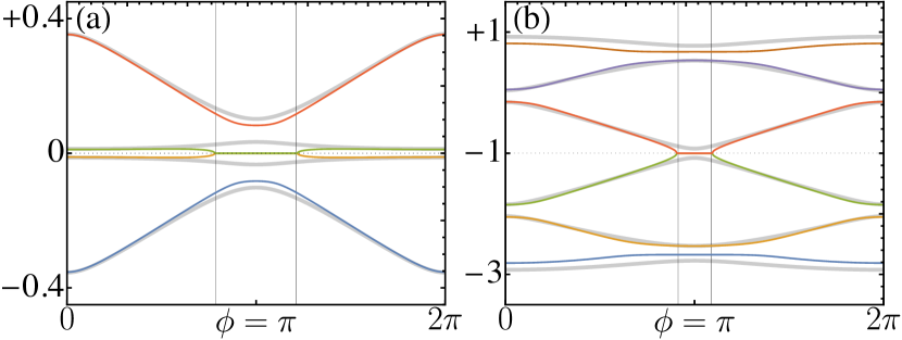
Figure S5-4: Supplemental plots for Fig. 1: (a) SNS junction and (b) normal metallic ring. The real parts of the low-energy spectra (colorful lines) vary with $\phi$, compared to the real spectra of the isolated system (gray lines). Their curvature has been altered by dissipation.

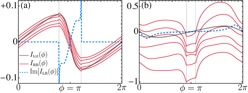
Figure S6-4: Supplemental plots for Fig. 2: (a) SNS junction and (b) normal metallic ring, where $I_{\rm iso}(\phi)$ (gray) acts as a reference. $I_{\textsc{rr}}(\phi)$ (red) shifts at different $j\in\mathbb{N}$, while $\mathrm{Im}[I_{\textsc{lr}}(\phi)]$ (dashed) displays the same divergent or finite curve as $\mathrm{Re}[I_{\textsc{lr}}(\phi)]$.

Figure S7-4: The current amplitudes variation with the coupling strength $\kappa$: (a) increases for small $\kappa$ in SNS junctions, but decreases for larger $\kappa$. (b) monotonically reduces as $\kappa$ increases in normal rings. The current amplitude $I^{\rm max}$ calculated by Eq. (1) closely matches the exact diagonalization $I^{\rm max}_{\rm tot}$ across all $\kappa$ examined.

Figure S8-4: Supplemental plots for Fig. 4, where $\mathrm{Im}\,\Pi(\phi,\omega)$ is solved by exact diagonalization of Eq. (III.2). We set $\eta=0.03$ for both (a) the SNS junction and (b) the normal mesoscopic ring. Same as the NH case, the level broadened effect is evident between two EPs (black lines). The other parameters are the same as in Fig. 1.

We provide additional low-energy spectra of NH systems in Fig. S6-4 as a supplement to Fig. 1, comparing them with the spectra of the decoupled Hermitian system. The slopes of these spectra indicate whether a mode’s contribution to the current is positive or negative. In the parameter setting of SNS junctions shown in Fig. S6-4(a), the EP-modes $\varepsilon_{\pm}$ do not dominate the current; instead, it is primarily contributed by the adjacent mode below. Because of their opposite slopes, in the Hermitian case, the lower-energy mode $\varepsilon_{-}$ has a negative contribution to the current, which is effectively counterbalanced by $\varepsilon_{+}$ due to level broadening in the NH case. In the normal ring illustrated in Fig. S6-4(b), however, we observe that any positive contributions from single-particle modes are consistently moderated by the dissipation-induced level broadening.

Fig. S6-4 is presented to complement the analysis of persistent currents discussed in Fig. 2. The RR-basis current $I_{\textsc{rr}}(\phi)$ exhibits peculiar shifts at different sites within the system, highlighting its violation of local conservation laws. Additionally, the imaginary part of the LR-basis current $\mathrm{Im}[I_{\textsc{lr}}(\phi)]$ is included to illustrate its similarity with its real part $\mathrm{Re}[I_{\textsc{lr}}(\phi)]$.

We further investigate how the current amplitudes $I^{\rm max}$ vary with coupling strength $\kappa/t$ across different regimes in Fig. S8-4. Panel (a) highlights the dual role of the thermal reservoir in the SNS junctions, where it enhances the current in the weak coupling regime but acts to suppress it under strong coupling conditions. Panel (b) shows a monotonic decrease in current amplitudes with increasing coupling strength in normal rings, aligning with the notion that dissipation suppresses the current amplitudes. In both models, the current amplitudes computed by Eq. (1) closely match those obtained through exact diagonalization across all examined coupling regimes, confirming its non-perturbative nature.

Fig. S8-4 presents supplemental data for Fig. 4. The current susceptibility calculated by Eq. (Non-Hermitian Persistent Current Transport) is consistent with Eq. (III.2) through exact diagonalization of the entire Hermitian system, including a large reservoir. This confirms the signatures of EPs and validates the effectiveness of our analytical approach in capturing the dynamics of NH systems.

References

Ashida et al. [2020]Y. Ashida, Z. Gong, and M. Ueda, Non-Hermitian physics, Adv. Phys. 69, 249 (2020).
Bergholtz et al. [2021]E. J. Bergholtz, J. C. Budich, and F. K. Kunst, Exceptional topology of non-Hermitian systems, Rev. Mod. Phys. 93, 015005 (2021).
Ding et al. [2022]K. Ding, C. Fang, and G. Ma, Non-Hermitian topology and exceptional-point geometries, Nat. Rev. Phys. 4, 745 (2022).
Xue et al. [2021]W.-T. Xue, M.-R. Li, Y.-M. Hu, F. Song, and Z. Wang, Simple formulas of directional amplification from non-Bloch band theory, Phys. Rev. B 103, L241408 (2021).
Hu et al. [2023]Y.-M. Hu, W.-T. Xue, F. Song, and Z. Wang, Steady-state edge burst: From free-particle systems to interaction-induced phenomena, Phys. Rev. B 108, 235422 (2023).
Li et al. [2023]B. Li, H.-R. Wang, F. Song, and Z. Wang, Non-Bloch dynamics and topology in a classical non-equilibrium process, arXiv:2306.11105 (2023).
Zou et al. [2024]J. Zou, S. Bosco, E. Thingstad, J. Klinovaja, and D. Loss, Dissipative Spin-Wave Diode and Nonreciprocal Magnonic Amplifier, Phys. Rev. Lett. 132, 036701 (2024).
Yu et al. [2022]Y. Yu, L.-W. Yu, W. Zhang, H. Zhang, X. Ouyang, Y. Liu, D.-L. Deng, and L.-M. Duan, Experimental unsupervised learning of non-Hermitian knotted phases with solid-state spins, npj Quantum Inf. 8, 1 (2022).
Chen et al. [2023]G. Chen, F. Song, and J. L. Lado, Topological Spin Excitations in Non-Hermitian Spin Chains with a Generalized Kernel Polynomial Algorithm, Phys. Rev. Lett. 130, 100401 (2023).
Ochkan et al. [2024]K. Ochkan, R. Chaturvedi, V. Könye, L. Veyrat, R. Giraud, D. Mailly, A. Cavanna, U. Gennser, E. M. Hankiewicz, B. Büchner, J. van den Brink, J. Dufouleur, and I. C. Fulga, Non-Hermitian topology in a multi-terminal quantum Hall device, Nat. Phys. 21, 1 (2024).
Yao and Wang [2018]S. Yao and Z. Wang, Edge States and Topological Invariants of Non-Hermitian Systems, Phys. Rev. Lett. 121, 086803 (2018).
Yang et al. [2020]Z. Yang, K. Zhang, C. Fang, and J. Hu, Non-Hermitian Bulk-Boundary Correspondence and Auxiliary Generalized Brillouin Zone Theory, Phys. Rev. Lett. 125, 226402 (2020).
Bernard and LeClair [2002]D. Bernard and A. LeClair, A Classification of Non-Hermitian Random Matrices, in Statistical Field Theories, NATO Science Series, edited by A. Cappelli and G. Mussardo (Springer Netherlands, Dordrecht, 2002) pp. 207–214.
Kawabata et al. [2019]K. Kawabata, K. Shiozaki, M. Ueda, and M. Sato, Symmetry and Topology in Non-Hermitian Physics, Phys. Rev. X 9, 041015 (2019).
Altland et al. [2021]A. Altland, M. Fleischhauer, and S. Diehl, Symmetry Classes of Open Fermionic Quantum Matter, Phys. Rev. X 11, 021037 (2021).
Golub and Van Loan [2013]G. H. Golub and C. F. Van Loan, Matrix Computations, 4th ed. (The Johns Hopkins University Press, Baltimore, 2013).
Wiersig [2014]J. Wiersig, Enhancing the Sensitivity of Frequency and Energy Splitting Detection by Using Exceptional Points: Application to Microcavity Sensors for Single-Particle Detection, Phys. Rev. Lett. 112, 203901 (2014).
Chen et al. [2017]W. Chen, Ş. Kaya Özdemir, G. Zhao, J. Wiersig, and L. Yang, Exceptional points enhance sensing in an optical microcavity, Nature 548, 192 (2017).
Hodaei et al. [2017]H. Hodaei, A. U. Hassan, S. Wittek, H. Garcia-Gracia, R. El-Ganainy, D. N. Christodoulides, and M. Khajavikhan, Enhanced sensitivity at higher-order exceptional points, Nature 548, 187 (2017).
Lau and Clerk [2018]H.-K. Lau and A. A. Clerk, Fundamental limits and non-reciprocal approaches in non-Hermitian quantum sensing, Nat. Commun. 9, 4320 (2018).
Lee et al. [2014]T. E. Lee, F. Reiter, and N. Moiseyev, Entanglement and Spin Squeezing in Non-Hermitian Phase Transitions, Phys. Rev. Lett. 113, 250401 (2014).
Ashida et al. [2017]Y. Ashida, S. Furukawa, and M. Ueda, Parity-time-symmetric quantum critical phenomena, Nat. Commun. 8, 15791 (2017).
Landi et al. [2022]G. T. Landi, D. Poletti, and G. Schaller, Nonequilibrium boundary-driven quantum systems: Models, methods, and properties, Rev. Mod. Phys. 94, 045006 (2022).
Gorini et al. [1976]V. Gorini, A. Kossakowski, and E. C. G. Sudarshan, Completely positive dynamical semigroups of N-level systems, J. Math. Phys. 17, 821 (1976).
Prosen [2008]T. Prosen, Third quantization: A general method to solve master equations for quadratic open Fermi systems, New J. Phys. 10, 043026 (2008).
McDonald and Clerk [2023]A. McDonald and A. A. Clerk, Third quantization of open quantum systems: Dissipative symmetries and connections to phase-space and Keldysh field-theory formulations, Phys. Rev. Res. 5, 033107 (2023).
Minganti et al. [2019]F. Minganti, A. Miranowicz, R. W. Chhajlany, and F. Nori, Quantum exceptional points of non-Hermitian Hamiltonians and Liouvillians: The effects of quantum jumps, Phys. Rev. A 100, 062131 (2019).
McDonald et al. [2022]A. McDonald, R. Hanai, and A. A. Clerk, Nonequilibrium stationary states of quantum non-Hermitian lattice models, Phys. Rev. B 105, 064302 (2022).
Song et al. [2019]F. Song, S. Yao, and Z. Wang, Non-Hermitian Skin Effect and Chiral Damping in Open Quantum Systems, Phys. Rev. Lett. 123, 170401 (2019).
Odashima et al. [2016]M. M. Odashima, B. G. Prado, and E. Vernek, Pedagogical introduction to equilibrium Green’s functions: Condensed-matter examples with numerical implementations, Rev. Bras. Ensino Fís. 39, 1 (2016).
Cayao and Sato [2023]J. Cayao and M. Sato, Non-Hermitian phase-biased Josephson junctions, arXiv:2307.15472 (2023).
Li et al. [2024]C.-A. Li, H.-P. Sun, and B. Trauzettel, Anomalous Andreev Spectrum and Transport in Non-Hermitian Josephson Junctions, arXiv:2307.04789 (2024).
Kornich [2023]V. Kornich, Current-Voltage Characteristics of the Normal Metal-Insulator-PT-Symmetric Non-Hermitian Superconductor Junction as a Probe of Non-Hermitian Formalisms, Phys. Rev. Lett. 131, 116001 (2023).
Note [0]See Supplemental Material at [URL will be inserted by publisher] for: () Green’s function and self-energy, () properties of the NH Fermi-Dirac distribution, () derivation of persistent current formula, and () extended numerical results on low-energy spectra, persistent currents, and current susceptibility, which includes Ref. [82].
Beenakker and van Houten [1992]C. W. J. Beenakker and H. van Houten, The Superconducting Quantum Point Contact, in Nanostructures and Mesoscopic Systems, edited by W. P. Kirk and M. A. Reed (Academic Press, 1992) pp. 481–497.
Chen and Zhai [2018]Y. Chen and H. Zhai, Hall conductance of a non-Hermitian Chern insulator, Phys. Rev. B 98, 245130 (2018).
Note [1]The term stems from the principal value (PV) in the integrand, which is typically disregarded in the literature [40], since in the weak coupling limit. However, PV plays a crucial role in correctly determining observables in EPs, which typically occur in the strong coupling regime.
Kawabata et al. [2023]K. Kawabata, T. Numasawa, and S. Ryu, Entanglement Phase Transition Induced by the Non-Hermitian Skin Effect, Phys. Rev. X 13, 021007 (2023).
Herviou et al. [2019]L. Herviou, N. Regnault, and J. H. Bardarson, Entanglement spectrum and symmetries in non-Hermitian fermionic non-interacting models, SciPost Phys. 7, 069 (2019).
Naghiloo et al. [2019]M. Naghiloo, M. Abbasi, Y. N. Joglekar, and K. W. Murch, Quantum state tomography across the exceptional point in a single dissipative qubit, Nat. Phys. 15, 1232 (2019).
Büttiker et al. [1983]M. Büttiker, Y. Imry, and R. Landauer, Josephson behavior in small normal one-dimensional rings, Phys. Lett. A 96, 365 (1983).
Lévy et al. [1990]L. P. Lévy, G. Dolan, J. Dunsmuir, and H. Bouchiat, Magnetization of mesoscopic copper rings: Evidence for persistent currents, Phys. Rev. Lett. 64, 2074 (1990).
Bluhm et al. [2009]H. Bluhm, N. C. Koshnick, J. A. Bert, M. E. Huber, and K. A. Moler, Persistent Currents in Normal Metal Rings, Phys. Rev. Lett. 102, 136802 (2009).
Bleszynski-Jayich et al. [2009]A. C. Bleszynski-Jayich, W. E. Shanks, B. Peaudecerf, E. Ginossar, F. von Oppen, L. Glazman, and J. G. E. Harris, Persistent Currents in Normal Metal Rings, Science 326, 272 (2009).
Carini et al. [1984]J. P. Carini, K. A. Muttalib, and S. R. Nagel, Origin of the Bohm-Aharonov Effect with Half Flux Quanta, Phys. Rev. Lett. 53, 102 (1984).
Browne et al. [1984]D. A. Browne, J. P. Carini, K. A. Muttalib, and S. R. Nagel, Periodicity of transport coefficients with half flux quanta in the Aharonov-Bohm effect, Phys. Rev. B 30, 6798 (1984).
Cheung et al. [1988]H.-F. Cheung, Y. Gefen, E. K. Riedel, and W.-H. Shih, Persistent currents in small one-dimensional metal rings, Phys. Rev. B 37, 6050 (1988).
Byers and Yang [1961]N. Byers and C. N. Yang, Theoretical Considerations Concerning Quantized Magnetic Flux in Superconducting Cylinders, Phys. Rev. Lett. 7, 46 (1961).
Note [2] for numerical results in the main text.
Akkermans et al. [1991]E. Akkermans, A. Auerbach, J. E. Avron, and B. Shapiro, Relation between persistent currents and the scattering matrix, Phys. Rev. Lett. 66, 76 (1991).
Note [3]To maintain a unified formalism across normal rings and SNS junctions, we adopt a constant and refrain from self-consistent calculations of observables for SNS junctions.
Note [4]In the range of moderate , the current amplitude may fluctuate in normal rings due to the shift of the effective Fermi level.
Trivedi and Browne [1988]N. Trivedi and D. A. Browne, Mesoscopic ring in a magnetic field: Reactive and dissipative response, Phys. Rev. B 38, 9581 (1988).
Ferrier et al. [2013]M. Ferrier, B. Dassonneville, S. Guéron, and H. Bouchiat, Phase-dependent Andreev spectrum in a diffusive SNS junction: Static and dynamic current response, Phys. Rev. B 88, 174505 (2013).
Dassonneville et al. [2013]B. Dassonneville, M. Ferrier, S. Guéron, and H. Bouchiat, Dissipation and Supercurrent Fluctuations in a Diffusive Normal-Metal–Superconductor Ring, Phys. Rev. Lett. 110, 217001 (2013).
Note [5]The four additional anomalous contributions are
Due to the local conservation law, is uniform and thus we set as the first site of in the calculation.
Riwar et al. [2016]R.-P. Riwar, M. Houzet, J. S. Meyer, and Y. V. Nazarov, Multi-terminal Josephson junctions as topological matter, Nat. Commun. 7, 1 (2016).
Pankratova et al. [2020]N. Pankratova, H. Lee, R. Kuzmin, K. Wickramasinghe, W. Mayer, J. Yuan, M. G. Vavilov, J. Shabani, and V. E. Manucharyan, Multiterminal Josephson Effect, Phys. Rev. X 10, 031051 (2020).
Coraiola et al. [2023]M. Coraiola, D. Z. Haxell, D. Sabonis, H. Weisbrich, A. E. Svetogorov, M. Hinderling, S. C. ten Kate, E. Cheah, F. Krizek, R. Schott, W. Wegscheider, J. C. Cuevas, W. Belzig, and F. Nichele, Phase-engineering the Andreev band structure of a three-terminal Josephson junction, Nat. Commun. 14, 6784 (2023).
Shen et al. [2021]P.-X. Shen, S. Hoffman, and M. Trif, Theory of topological spin Josephson junctions, Phys. Rev. Res. 3, 013003 (2021).
Moskalets and Büttiker [2002]M. Moskalets and M. Büttiker, Floquet scattering theory of quantum pumps, Phys. Rev. B 66, 205320 (2002).
Blaauboer [2002]M. Blaauboer, Charge pumping in mesoscopic systems coupled to a superconducting lead, Phys. Rev. B 65, 235318 (2002).
Becerra et al. [2023]V. F. Becerra, M. Trif, and T. Hyart, Quantized Spin Pumping in Topological Ferromagnetic-Superconducting Nanowires, Phys. Rev. Lett. 130, 237002 (2023).
Shen et al. [2023]P.-X. Shen, V. Perrin, M. Trif, and P. Simon, Majorana-magnon interactions in topological Shiba chains, Phys. Rev. Res. 5, 033207 (2023).