Quantum Dynamic Programming

Abstract

We introduce a quantum extension of dynamic programming, a fundamental computational method for efficiently solving recursive problems using memory. Our innovation lies in showing how to coherently generate unitaries of recursion steps using memorized intermediate quantum states. We find that quantum dynamic programming yields an exponential reduction in circuit depth for a large class of fixed-point quantum recursions, including a known recursive variant of the Grover’s search. Additionally, we apply quantum dynamic programming to a recently proposed double-bracket quantum algorithm for diagonalization to obtain a new protocol for obliviously preparing a quantum state in its Schmidt basis, providing a potential pathway for revealing entanglement structures of unknown quantum states.

Introduction.—Access to placeholder memory can drastically reduce computation runtime. For example, there is an exponential difference in computing the classic Fibonacci sequence with or without placeholder memory. Should one attempt it directly from the recursive definition

$$F(n)=F(n-1)+F(n-2),\qquad n\geq 2,$$ (1)

starting with $F(0)=0$ and $F(1)=1$, it is quickly realized that in order to compute $F(N)$ naively, we need to compute $F(N-2)$ twice because it appears in the expression for $F(N)$ and also for $F(N-1)$. In turn computing $F(N-2)$ requires two computations of $F(N-4)$, and so on. This leads to $\mathcal{O}(2^{N})$ additions to arrive at $F(N)$. Fortunately, one can mitigate this computational overhead by the elegant solution of memoization [1], i.e. using classical memory to store values of intermediate states $F(n)$, and retrieving $F(n)$ whenever necessary. The program then contains an explicit section (e.g. a memory) that changes with time and $F(N)$ is computed in $\mathcal{O}(N)$ time. Such strategies are known as dynamic programming [2, 3], and they utilize memory calls of the appropriate quantity to yield vastly shorter runtime than re-computations.

Memoization is more difficult in quantum computing than for classical computers because the readout of a quantum state $\rho$ renders it useless for future ‘retrieval’. As opposed to classical computing, this cannot be circumvented by the cloning of information [4]. Nonetheless, we will show that quantum dynamic programming, i.e. involving memoization in quantum algorithms, remains strategically the right choice and can lead to drastic circuit depth reductions, en par with the classic example of computing Fibonacci numbers.

Due to the no-cloning theorem, quantum memory is ‘consumed’ upon each ‘retrieval’, necessitating the preparation of multiple independent copies of an intermediate state. Hence, to achieve reductions in circuit depth, one needs circuits with a larger width. The crucial difference to the precomputation approaches [5, 6] emerges here; our memory states are not given, but we prepare them as a result of previous recursion steps. The localized structure of the arising circuits alleviates the difficulties associated with the large width requirement. Quantum memoization operates by partitioning a large computational task into smaller and independent state preparation circuits, much simpler than the full task and capable of being executed in parallel. Furthermore, the quantum recursions of interest exhibit strongly attractive fixed-points, i.e. the task at hand includes an intrinsic stabilizing effect so that, if sufficiently small, errors of the intermediate states do not wreck the quantum computation. The local modularity and intrinsic stabilization make such recursions a natural use-case for distributed quantum computing [7, 8, 9], when implemented using quantum dynamic programming.

Any protocol must conclude within the coherence time scales of the quantum processor; therefore, among circuits achieving the same task, it is strategic to select those with minimized depth rather than width. Quantum dynamic programming radically alters the circuit structure to achieve just that, i.e. the key characteristic — circuit depth — gets shortened through quantum memoization. We show that this underexplored design principle can enable successful quantum computations where ordinary proposals would fail.

Quantum recursion steps consist of unitary transformations $\hat{U}^{(\rho_{n})}$ that explicitly depend on past states $\rho_{n}$,

$$\rho_{n+1}=\hat{U}^{(\rho_{n})}\rho_{n}\left(\hat{U}^{(\rho_{n})}\right)^{\dagger}\ .$$ (2)

Importantly, $\rho_{n}$ may be unknown, so in each recursion step $n$, the transformation must be implemented ‘obliviously’. Thus, Eq. (2) entails a key challenge for using memoization in quantum algorithms: How can an intermediate state $\rho_{n}$ feed back into the ‘knobs’ of the quantum computer and determine the subsequent gate applications? In other words, how can we use quantum data $\rho_{n}$ as a quantum instruction [10] for $\hat{U}^{(\rho)}$?

In this manuscript, we systematically address this challenge for a class of recursion unitaries $\hat{U}^{(\rho)}$ by employing quantum memory-calls. Specifically, we apply it to i) a known quantum algorithm, namely recursive Grover’s search [11], and ii) a dynamic implementation of recently proposed quantum recursions for diagonalization [12], leading to a quantum algorithm for transforming a state into its Schmidt basis without knowledge of the state itself. With this, we establish that a quantum-mechanical version of dynamic programming is not only a strategic conceptual framework but also highly applicable.

Memory-calls in quantum recursions.—Suppose we desire to implement a unitary that depends on a state $\rho_{n}$, as in Eq. (2), but we do not know $\rho_{n}$ and only have access to copies of $\rho_{n}$. To characterize such unitaries, let $\hat{\mathcal{N}}$ be a map from Hermitian quantum instruction states $\rho$ to Hermitian operators $\hat{\mathcal{N}}(\rho)$. Thus, $\hat{\mathcal{N}}$ is Hermitian-preserving and $e^{i\hat{\mathcal{N}}(\rho)}$ is unitary as required. We say that a quantum recursion contains a single memory-call, if it is of the form

$$\hat{U}^{(\hat{\mathcal{N}},\rho)}=\hat{V}_{2}e^{i\hat{\mathcal{N}}(\rho)}\hat{V}_{1}\ .$$ (3)

Here $\hat{V}_{1},\hat{V}_{2}$ are static unitaries, independent of the instruction state $\rho$. That state can vary dynamically so the memory-call unitary $e^{i\hat{\mathcal{N}}(\rho)}$ is dynamic too.

Quantum programming with memory-calls consists of choosing $\hat{\mathcal{N}}$ appropriately. For example $\hat{\mathcal{N}}(\rho)=t\rho$ corresponds to density matrix exponentiation [13, 14] and enables a framework for universal quantum computation. Another example is $\hat{\mathcal{N}}(\rho)=[\hat{D},\rho]$, the commutator of the input with a fixed operator $\hat{D}$ which facilitates diagonalization [12], as we will see in our example algorithm. Eq. (3) naturally generalizes to a recursion with multiple memory-calls

$$\hat{U}^{(\{\hat{\mathcal{N}}\},\rho)}=\hat{V}_{L}e^{i\hat{\mathcal{N}}_{L}(\rho)}\hat{V}_{L-1}e^{i\hat{\mathcal{N}}_{L-1}(\rho)}\ldots\hat{V}_{1}e^{i\hat{\mathcal{N}}_{1}(\rho)}\hat{V}_{0}\ .$$ (4)

We will next discuss a recursive variant of Grover’s algorithm [15] whose recursion steps are exactly in this form.

Unfolding quantum recursions—The nested fixed-point Grover search [11] has the recursive structure $|{\psi_{n+1}}\rangle=\hat{\Gamma}^{(\psi_{n})}_{L}|{\psi_{n}}\rangle$, where each step consists of alternating reflections

$$\hat{\Gamma}^{(\psi)}_{L}=\displaystyle\prod_{i=1}^{L}\hat{E}^{(\psi)}_{\alpha_{i}}\hat{E}^{(\tau)}_{\beta_{i}}.$$ (5)

Here $\hat{E}^{(\sigma)}_{s}=e^{-is\sigma}=\mathmybb{1}-(1-e^{-is})|{\sigma}\rangle\!\langle{\sigma}|$ are reflection unitaries and $\tau$ is the pure target state which the algorithm aims to output. In the recursion, Eq. (5) depends dynamically on any intermediate state $\psi_{n}$. The set of predetermined angles $\{\alpha_{i},\beta_{i}\}_{i=1}^{L}$ optimizes the procedure and if we set $\hat{\mathcal{N}}_{i}(\rho)=-\alpha_{i}\rho$ and $\hat{V}_{i-1}=\hat{E}^{(\tau)}_{\beta_{i}}$, $\hat{V}_{L}=\mathmybb{1}$ then Eq. (5) is in form of Eq. (4).

Ref. [11] proposed to use re-computations to prepare the state $|{\psi_{N}}\rangle=\hat{\Gamma}^{(\psi_{N-1})}_{L}\ldots\hat{\Gamma}^{(\psi_{0})}_{L}|{\psi_{0}}\rangle\approx|{\tau}\rangle$. No placeholder memory beyond the register storing $|{\psi_{0}}\rangle$ is involved; hence, we call it a zero-memory approach. Consider the simplest case $L=1$, when the recursion involves only one memory-call. For the second recursion step we have $|{\psi_{2}}\rangle=\hat{\Gamma}^{(\psi_{1})}_{1}\hat{\Gamma}^{(\psi_{0})}_{1}|{\psi_{0}}\rangle$, with $\hat{\Gamma}^{(\psi_{1})}_{1}$ and $\hat{\Gamma}^{(\psi_{0})}_{1}$ defined in Eq. (5). The reflection around $\psi_{1}$ is not directly available but we assume that we can reflect around $\psi_{0}$ and $\tau$. Crucially $\psi_{1}=\hat{\Gamma}^{(\psi_{0})}_{1}{\psi_{0}}\bigl{(}\hat{\Gamma}^{(\psi_{0})}_{1}\bigr{)}^{\dagger}$ implies

$$\hat{E}^{(\psi_{1})}_{\alpha_{1}}=\hat{\Gamma}^{(\psi_{0})}_{1}\hat{E}^{(\psi_{0})}_{\alpha_{1}}\left(\hat{\Gamma}^{(\psi_{0})}_{1}\right)^{\dagger}\ .$$ (6)

Consequently, we can implement $\hat{\Gamma}^{(\psi_{1})}_{1}=\hat{E}^{(\psi_{1})}_{\alpha_{1}}\hat{E}^{(\tau)}_{\beta_{1}}$ using the available relfections and obtain $|{\psi_{2}}\rangle$. For further recursion steps we proceed analogously, each time obtaining a sequence of unitaries which involve reflections only around $\psi_{0}$ and $\tau$.

The key step is the covariance Eq. (6). The same approach works for any $L$ when there are multiple memory-calls, and in Sec. II.1 of Supplemental Materials we generalize this zero-memory procedure to multiple memory-call recursion steps where polynomials $f_{k}$ are used in lieu of $\hat{\mathcal{N}}_{k}$ for Eq. (4).

We refer to this strategy of executing quantum recursions as ‘unfolding’ [11, 12]. Its severe drawback is that it needs an exponentially deep circuit – a consequence of applying $\hat{U}^{(\rho_{n-1})}$ and its inverse $L$ times to implement $\hat{U}^{(\rho_{n})}$. Consequently, the circuit depth for evaluating the $n$th recursion step scales as $(2L)^{n}$, in units of the gate complexity needed for an initial recursion step. Unfolding is analogous to a re-computation of intermediate states $\rho_{n}$ and thus is static rather than dynamic.

Memory-usage queries.—We propose to prepare memory-call unitaries $e^{i\hat{\mathcal{N}}(\rho)}$ by dynamically invoking memory. The execution via memoization means that we apply a unitary operation $\mathcal{Q}$ on two registers, the working register containing $\sigma$ and the memory register containing the instruction state $\rho$. After the action of $\mathcal{Q}$, we discard the memory register, while the working state becomes transformed by a dynamic operation instructed by $\rho$. We dub this protocol a memory-usage query, and remark that $\mathcal{Q}$ is oblivious to the states $\rho$ and $\sigma$.

More specifically, we need a way to apply the unitary channel $\hat{\mathbf{E}}^{(\hat{\mathcal{N}},\rho)}$ of $e^{i\hat{\mathcal{N}}(\rho)}$ to a working state $\sigma$:

$$\hat{\mathbf{E}}^{(\hat{\mathcal{N}},\rho)}(\sigma)=e^{i\hat{\mathcal{N}}(\rho)}(\sigma)e^{-i\hat{\mathcal{N}}(\rho)}\ .$$ (7)

A key observation is that this map can be approximately implemented by using multiple copies of the (unknown) state $\rho$ [14, 16]. In particular, the Choi matrix of $\hat{\mathcal{N}}$ leads to the operation $\mathcal{Q}$ oblivious to $\rho$, such that the memory-usage query approximates Eq. (7) [16]. Let us denote $\hat{N}=\Lambda^{\transp_{1}}$, the partial transpose of the Choi matrix $\Lambda$ of $\hat{\mathcal{N}}$ (see Supplemental Materials Section II.2 for an explicit expression). Then, consider a map defined by

$$\hat{\mathcal{E}}^{(\hat{\mathcal{N}},\rho)}_{s}(\sigma)=\operatorname{Tr}_{1}\left[e^{-i\hat{N}s}\left(\rho\otimes\sigma\right)e^{i\hat{N}s}\right]\ ,$$ (8)

where $\mathcal{Q}=e^{-i\hat{N}s}$ is oblivious, i.e. independent of both the memory and working registers. We ‘consume’ the state $\rho$ as we trace out the memory register. Eq. (8) is a single query because we use one copy of $\rho$; if this procedure is repeated $M$ times with $s=\frac{1}{M}$, i.e. if $M$ queries consuming $M$ copies of $\rho$ are performed, we obtain

$$\hat{\mathcal{E}}^{(\hat{\mathcal{N}},\rho,M)}_{\text{QDP}}\coloneq\left(\hat{\mathcal{E}}^{(\hat{\mathcal{N}},\rho)}_{1/M}\right)^{M}=\hat{\mathbf{E}}^{(\hat{\mathcal{N}},\rho)}+\mathcal{O}\left(1/{M}\right)\ .$$ (9)

Quantum dynamic programming.—We define quantum dynamic programming (QDP) to consist of making memory-usage queries on copies of $\rho_{n}$ to approximate a recursion step towards $\rho_{n+1}$. More specifically, consider initializing a quantum program with $\sigma_{0}=\rho_{0}$, and defining the QDP iteration

$$\sigma_{n+1}=\hat{\mathcal{E}}^{(\hat{\mathcal{N}},\rho,M)}_{\text{QDP}}(\sigma_{n})\ .$$ (10)

From Eq. (9), we see that Eq. (10) approximates a single memory-call recursion (Eq. (3) with $\hat{V}_{1}=\hat{V}_{2}=\mathmybb{1}$) by $M$ memory-usage queries. In general, for recursions with multiple memory-calls, we define the QDP iteration as replacing all memory-calls $e^{i\hat{\mathcal{N}}(\rho)}$ by total $M$ memory-usage queries.

Trading circuit depth for width with QDP.—To prepare one copy of $\sigma_{1}$, we make $M$ memory-usage queries using $\sigma_{0}$ as an instruction. In other words, the first step consumes $M$ root state copies. Likewise, to prepare one copy of $\sigma_{2}$, we need $M^{2}$ copies of $\sigma_{0}$; thus, the iteration of Eq. (10) consumes $M^{n}$ copies of the root state. Although the circuit width grows exponentially with $n$, the circuit depth remains polynomial: the preparation of multiple copies of instruction states is done in parallel, and the maximum depth is equal to performing $nM$ memory-usage queries. In comparison, unfolding requires a circuit depth exponential in $n$ and has a constant width.

Before declaring an exponential depth reduction over unfolding, however, we must ensure that each memory-call approximation in QDP is sufficiently accurate to prepare the final state $\sigma_{N}$ within the same error threshold as unfolding. We next discuss the number of memory-usage queries $M$ needed for that.

Exponential depth reduction with QDP.—Aiming for an exact solution of quantum recursions is unrealistic because of inaccuracies prevalent in quantum circuit compilation, e.g. due to a finite $M$ in Eq. (9), among others. We next discuss the accuracy of QDP when allowing for errors in the preparation of the root state $\sigma_{0}$ and deviations from the exact recursion steps.

By Eq. (9), $M=\mathcal{O}(1/\epsilon)$ suffices for $\|\sigma_{1}-\rho_{1}\|_{1}\leq\mathcal{O}(\epsilon)$. The next step might have an amplified deviation because the second recursion step $\sigma_{2}=\hat{\mathcal{E}}^{(\hat{\mathcal{N}},\sigma_{1},M)}_{\text{QDP}}(\sigma_{1})$ is instructed by $\sigma_{1}$ and not $\rho_{1}$. Indeed, triangle inequality gives $\|\sigma_{2}-\rho_{2}\|_{1}\leq\mathcal{O}(M\epsilon)$; see Sec. II of Supplemental Materials for the full analysis. We shall next characterize a sufficient condition for errors on quantum instructions not to propagate destructively, indicating that this upper bound need not be realized.

It turns out that if the first few steps are sufficiently accurate, implementing the next steps benefits from the stabilization property of the recursions itself. Indeed, for many fixed-point recursions (e.g. by use of the Polyak-Łojasiewicz inequality for gradient descent iterations [17] or by asymptotic stability analysis of time-discrete dynamical systems [18]) exponential convergence can be obtained.

For a quantum recursion, exponential convergence would read

$$\|\rho_{N}-\rho_{\infty}\|_{1}\leq\alpha^{N}\|\rho_{0}-\rho_{\infty}\|_{1}\ ,$$ (11)

for some $\alpha<1$. However, we must assume that i) a stable fixed-point $\rho_{\infty}$ is reached for $N\rightarrow\infty$, ii) it is ‘spectrally’ unique, i.e. any two root states of the recursion $\rho_{0}$ and $\rho_{0}^{\prime}$ with the same spectrum have the same fixed-point $\rho_{\infty}=\rho_{\infty}^{\prime}$, and finally iii) the fixed-point attracts all states sufficiently strongly to tolerate small implementation errors. The latter property is made explicit in Sec. III of Supplemental Materials and plays the role of deciding the convergence rate similar to $\alpha$ in Eq. (11).

We say that a quantum recursion satisfying conditions i,ii,iii) has fast spectral convergence. Conversely, the absence of iii) renders the recursion unstable, suggesting its lack of physical relevance; protocols achievable in nature must be resilient to small perturbations. In such cases quantum computation cannot be expected to be both efficient and successful, potentially necessitating infinite precision and thus infinite resources for convergence. Implementing recursions with unfolding is subject to similar stability requirements. Thus, we should focus on recursions with fast spectral convergence; otherwise, the computational task is ill-conditioned.

If a recursion exhibits fast spectral convergence, QDP delivers an exponential depth reduction compared to unfolding:

Theorem 1 (QDP, non-technical).

Suppose that the quantum recursion satisfies fast spectral convergence. If we implement $N$ recursion steps of the form Eq. (4), by replacing each memory-call by $\mathcal{O}(N\epsilon^{-1})$ memory-usage queries, the final state $\sigma_{N}$, such that

$$\|\sigma_{N}-\rho_{N}\|_{1}\leq\epsilon,$$ (12)

can be achieved with a circuit of depth $\mathcal{O}(N^{2}\epsilon^{-1})$. Here, $\rho_{N}$ is the exact solution to the recursion.

The full, technical version of Theorem 1 can be found in Supplemental Materials Section III, as Theorem 9.

Exponential width increase mitigation.—Realistically, quantum devices can neither execute exponentially many sequential gates nor operate on exponentially many qubits simultaneously. Therefore, it becomes inevitable to consider a hybrid approach, where QDP is initiated after several rounds of unfolding recursions. This hybrid approach strategically allocates the exponential factor between circuit depth and width, without overburdening either. One can envisage a scheme where $N_{1}$ recursions unfold, using a circuit of depth $e^{\mathcal{O}(N_{1})}$, nearly reaching the device’s limit. These unfolding steps, conducted in parallel to exploit maximum width, yield $M$ copies of intermediate states $\rho_{N_{1}}$. Subsequently, QDP takes over, executing an additional $N_{2}$ recursions to attain the final state $\sigma_{N_{1}+N_{2}}$. This strategy maximizes the device’s capacity, which would have otherwise produced either $\rho_{N_{1}}$ without QDP or $\sigma_{N_{2}}$ without unfolding.

Another advantage of adopting a hybrid strategy arises from inherent implementation imperfection that QDP entails. As will be demonstrated in the Grover search example, this might limit the initial states to those already possessing certain favorable properties. In the hybrid approach, we effectively steer the ineligible initial state to meet the requirements imposed by QDP through initial rounds of unfolding recursions.

Example 1: Grover search.—Theorem 1, when applied to the fixed-point Grover search, indicates a circuit depth scaling of $\mathcal{O}(N^{2}\epsilon^{-1})$. However, a more refined analysis reveals a better scaling of $\mathcal{O}(N\epsilon^{-1})$. Specifically, we analyze a QDP implementation of the nested fixed-point Grover search [11], a recursive variant of Grover’s fixed-point algorithm [15], characterized by Eq. (5). This operation transforms the input state into a state closer to the target:

$$\left\lVert\tau-\hat{\Gamma}^{(\psi)}_{L}\psi\left(\hat{\Gamma}^{(\psi)}_{L}\right)^{\dagger}\right\rVert_{1}<\bigg{\lVert}\tau-\psi\bigg{\rVert}_{1}\ .$$ (13)

For a single recursion step, as analyzed in Ref. [11], the output state with a distance $\delta$ to the target state is achieved by $L=\mathcal{O}(\log(1/\delta))$. The circuit depth $\mathcal{O}(L)=\mathcal{O}(\log(1/\delta))$ matches that of the optimal Grover search [19, 20].

Ref. [11] additionally shows that the same distance $\delta$ can be achieved by executing $N$ recursions with shorter length $L=\mathcal{O}((\log(1/\delta))^{\frac{1}{N}})$, following the recurrence relation $|{\psi_{n+1}}\rangle=\hat{\Gamma}^{(\psi_{n})}_{L}|{\psi_{n}}\rangle$ as discussed earlier. The recursion is implemented through unfolding, and the total circuit depth for $N$ iterations scales exponentially as $\mathcal{O}((2L+1)^{N})=\mathcal{O}(\log(1/\delta))$, asymptotically equivalent to the non-recursive version of the algorithm; refer to Supplemental Materials Sec. IV.1 for a self-contained discussion. In contrast, our QDP implementation reduces the circuit depth to $\mathcal{O}(N)$, implying an exponential runtime speedup for the implementation of Grover search.

Theorem 2 (Efficient QDP Grover search, non-technical).

Suppose that the initial state $\psi_{0}$ is sufficiently close to the target state $\tau$ for the nested fixed-point Grover search. By implementing $N$ recursion steps via QDP, one can prepare the final state that is $\epsilon$-close to that of $N$ exact recursion steps. This implementation uses a circuit of depth $\mathcal{O}(N\epsilon^{-1})$ and $e^{\mathcal{O}(N)}$ copies of the initial state $\psi_{0}$.

The technical version of Theorem 2 is Theorem 21 in Supplemental Materials Sec. IV, and we provide the detailed analysis there. The circuit depth scaling is better than in Theorem 1 thanks to an additional protocol based on Ref. [21] which probabilistically reduces the mixedness of a state, while preserving its eigenvectors.

The requirement of small $\lVert\tau-\psi_{0}\rVert_{1}$ stems from approximate memory-calls in QDP: when the initial overlap is too small, the contraction in the distance to the target state may be insufficient to offset the implementation error, i.e. the algorithm lacks fast spectral convergence. If the given initial state does not meet this criterion, a hybrid approach should be employed instead.

Example 2: Oblivious Schmidt decomposition.—For any bi-partite pure state $|{\psi_{0}}\rangle\in\mathcal{H}_{A}\otimes\mathcal{H}_{B}$, there exist local unitaries $\hat{V}_{A}$ and $\hat{V}_{B}$ that simplify the Schmidt decomposition to be in the computational basis, i.e. $\hat{V}_{A}\otimes\hat{V}_{B}|{\psi_{0}}\rangle=\sum_{k=1}^{D}\sqrt{\lambda_{k}}|{k}\rangle\otimes|{k}\rangle$, where $\{\lambda_{k}\}_{k}$ denotes the Schmidt spectrum [22, 23]. This decomposition is of paramount importance for quantum information theory but of limited use as a practical technique. The main obstacle is that $\hat{V}_{A}$ and $\hat{V}_{B}$ depend on the state $|{\psi_{0}}\rangle$; thus, it seemed necessary to learn $|{\psi_{0}}\rangle$ first, classically compile the unitaries, and implement them in physical devices. Instead, QDP allows the oblivious execution of the Schmidt decomposition, without requiring a classical description of $|{\psi_{0}}\rangle$, by applying double-bracket iterations [12] to the reduced state of $|{\psi_{0}}\rangle$.

We describe the gist of the algorithm here, and expound further in Supplemental Materials Section V. Let $\hat{D}$ be a diagonal operator on subsystem $A$. The oblivious Schmidt decomposition recursion is defined as $|{\psi_{n+1}}\rangle=\hat{U}^{(\psi_{n})}|{\psi_{n}}\rangle$, where

$$\hat{U}^{(\psi_{n})}=e^{s[\hat{D},\rho_{n}^{(A)}]}\otimes\mathmybb{1}_{B}\ ,$$ (14)

and $\rho_{n}^{(A)}=\operatorname{Tr}_{B}[|{\psi_{n}}\rangle\!\langle{\psi_{n}}|]$ is the reduced density matrix after $n$ steps. In other words, it is a single memory-call type recursion with $\hat{\mathcal{N}}(\rho)=-is[\hat{D},\rho]$ that is Hermitian-preserving. If $\hat{D}$ has a non-degenerate spectrum and $s$ is small [24], the reduced state of the fixed-point is a diagonal state isospectral to $\rho_{0}^{(A)}$. Under the same condition, exponential convergence can be proven, which is conceptually similar to fast spectral convergence and is a feature of gradient flows in general [25]. One can adapt $\hat{D}_{n}$ in every step variationally, and then in practice, a non-degenerate spectrum is not required [12].

In QDP implementation, Eq. (14) is generated by coupling many copies of $\rho_{n}^{(A)}$, prepared independently each time starting from $\rho_{0}^{(A)}=\operatorname{Tr}_{B}[|{\psi_{0}}\rangle\!\langle{\psi_{0}}|]$. After $N$ iterations, at which $\rho_{N}^{(A)}$ is sufficiently diagonal, the Schmidt spectrum can be extracted via measurements in the computational basis.

Obtaining the Schmidt spectrum of a density matrix can be done also by the ‘replica’ method [26], i.e. by measuring $\operatorname{Tr}(C_{A}\psi_{AB}^{\otimes k})=\operatorname{Tr}\rho_{A}^{k}$, where $C_{A}|{i_{1},i_{2},\dots,i_{k}}\rangle_{A}=|{i_{k},i_{1},i_{2},\dots,i_{k-1}}\rangle_{A}$ is the cycle permutation of $k$ copies of the subsystem $A$ and performing classical data analysis of $\operatorname{Tr}\rho_{A}^{k}$ for $k=2,\dots,d$. Besides requiring exponentially many swap operations for $k=d$, the replica approach is incoherent. The major strength of oblivious Schmidt decomposition is to provide coherently the bipartite quantum state $\sum_{k}\sqrt{\lambda_{k}}|{k}\rangle\otimes|{k}\rangle$ in the computational basis. This is useful, e.g. for entanglement distillation of an unknown state $\psi$, which contrasts to the standard setting [27] where the information about the initial state is necessary for compiling appropriate local operations. Ref. [28] showed that the same asymptotic rate (characterized by entanglement entropy) can be achieved for the oblivious setting. Oblivious Schmidt decomposition may not realize such an optimal rate but provides a constructive way of oblivious entanglement distillation, which comes with an explicit circuit construction.

Conclusion and outlook.— We introduced the general framework of quantum dynamic programming that, similarly to the classical version, leverages placeholder memory to achieve runtime reductions. We found that it is capable of implementing a broad class of quantum recursions involving memory-calls. Whenever fixed-points of recursions are sufficiently well-behaved, we showed that QDP yields accurate results with polynomial depth. This represents an exponential speed-up over the previously proposed zero-memory implementations by ‘unfolding’ [11, 12]. Our approach introduces a new possibility of balancing circuit depth and width, facilitating the implementation of quantum recursions in real devices. QDP casts quantum recursions into circuits with many parallel but few sequential operations and renders them suitable as a central use-case for distributed quantum computing [7, 8, 9].

For QDP applications involving only a marginal amount of quantum coherence, an approximate cloning heuristic [29] could be used: these cases would potentially enjoy an exponential speed-up without inflating the circuit width. Nevertheless, quantitative bounds relating the coherence of input quantum states to cloning fidelity are currently unknown [30]. It is also unclear how far the presence of coherence could be viewed as a signature of quantum simulation hardness, generalizing to quantum recursions the role of entanglement in tensor network simulations [31]. Thorough investigations on the role of coherence in QDP will make an interesting future direction.

We do not know of quantum algorithms for which QDP facilitates a rigorous computational advantage over classical algorithms. These may appear in settings robust against imprecision of unitary implementations, similar to those present in diagonalizing double-bracket iterations [24, 25, 12]. Indeed, QDP allows us to add oblivious Schmidt decomposition to the available quantum algorithmic toolkit. It is our hope that once it will be feasible to experimentally implement memory-usage queries with high fidelity, then oblivious Schmidt decomposition and QDP in general will facilitate practical state preparations that will advance our knowledge about quantum properties of materials, e.g. magnets or superconductors.

Acknowledgements.—JS, MG, and NN are supported by the start-up grant for Nanyang Assistant Professorship of Nanyang Technological University, Singapore, awarded to Nelly H. Y. Ng. MG additionally acknowledges support through the Presidential Postdoctoral Fellowship of the Nanyang Technological University. RT acknowledges the support of JSPS KAKENHI Grant Number JP23K19028, JST, CREST Grant Number JPMJCR23I3, Japan, and the Lee Kuan Yew Postdoctoral Fellowship of Nanyang Technological University Singapore.

Supplemental Materials for “Quantum Dynamic Programming”

I Preliminaries and distance measures

We denote Hilbert spaces as $\mathcal{H}$ and the set of quantum states having support in $\mathcal{H}$ as $\mathcal{S}(\mathcal{H})$, which is a subset of $\mathcal{B}(\mathcal{H})$, the set of generic bounded operators acting on $\mathcal{H}$. When not specified, quantum channels are assumed to map $\mathcal{S}(\mathcal{H})\rightarrow\mathcal{S}(\mathcal{H})$. The identity operator acting on $\mathcal{H}$ is denoted as $\mathmybb{1}$, whereas the identity map from $\mathcal{S}(\mathcal{H})$ to $\mathcal{S}(\mathcal{H})$ is denoted as $\operatorname{id}$.

A few different distance measures between operators and channels are utilized in this paper. The trace norm distance between two normal operators acting on the same space $\mathcal{B}(\mathcal{H})$ is defined to be

$$\frac{1}{2}\lVert\hat{A}-\hat{B}\rVert_{1}\coloneq\frac{1}{2}\operatorname{Tr}\left[\sqrt{(\hat{A}-\hat{B})^{\dagger}(\hat{A}-\hat{B})}\right]\ .$$ (15)

Between two pure states $\psi$ and $\phi$, the trace norm distance can be written with respect to their overlap as $\frac{1}{2}\left\lVert\psi-\phi\right\rVert_{1}=\sqrt{1-\lvert\langle{\psi}|{\phi}\rangle\rvert^{2}}$. Another measure uses the Hilbert-Schmidt norm and is defined as

$$\frac{1}{2}\lVert\hat{A}-\hat{B}\rVert_{2}\coloneq\frac{1}{2}\sqrt{\operatorname{Tr}\left[(\hat{A}-\hat{B})^{\dagger}(\hat{A}-\hat{B})\right]}\ .$$ (16)

The operator norm of a normal operator $\hat{A}$ is defined to be $\|\hat{A}\|_{\infty}=\max\{|\lambda_{j}|\}$, where $\lambda_{j}$ are eigenvalues of $\hat{A}$; likewise, the operator norm distance between two normal operators $\hat{A}$ and $\hat{B}$ is $\frac{1}{2}\|\hat{A}-\hat{B}\|_{\infty}$.

One can define distances between two quantum channels $\mathcal{S}(\mathcal{H})\rightarrow\mathcal{S}(\mathcal{H}^{\prime})$, leveraging on operator distances. The trace norm distance between two quantum channels $\Phi_{1},\Phi_{2}$ is defined as the maximum distance between the outputs of two channels given an identical input state, i.e.

$$\frac{1}{2}\|\Phi_{1}-\Phi_{2}\|_{\rm Tr}\coloneq\frac{1}{2}\max_{\varrho\in\mathcal{S}(\mathcal{H})}\left\lVert\Phi_{1}(\varrho)-\Phi_{2}(\varrho)\right\rVert_{1}\ .$$ (17)

The diamond norm distance between $\Phi_{1},\Phi_{2}$ is a stronger measure of distance between channels, because it further optimizes over input states that can be entangled with an external reference,

$$\frac{1}{2}\|\Phi_{1}-\Phi_{2}\|_{\diamond}\coloneq\frac{1}{2}\max_{\varrho\in\mathcal{S}(\mathcal{H}\otimes\mathcal{H})}\left\lVert(\Phi_{1}\otimes\operatorname{id})(\varrho)-(\Phi_{2}\otimes\operatorname{id})(\varrho)\right\rVert_{1}\ .$$ (18)

It is useful to note that the diamond norm distance always upper bounds the trace norm distance, $\|\Phi_{1}-\Phi_{2}\|_{\diamond}\geq\|\Phi_{1}-\Phi_{2}\|_{\rm Tr}$.

For both operators and channels, norms $\|\cdotB\|$ with no subscript denotes that some unitary invariant norm (including trace norm, operator norm, etc.) is used.

II Locally accurate implementations

Consider a quantum recursion defined by Eq. (7) with the root state $\sigma_{0}$. The exact implementation of memory-calls in recursion steps would lead to a sequence of states $\rho_{0},\rho_{1},\ldots$. We need to consider the situation where each recursion step consists of approximations of memory-calls.

For example, consider the QDP implementation. If we continue the recursion with approximate memory-calls, at $(n-1)$th recursion step, the instruction states available to us in the memory register are $\sigma_{n}$, which might be different from the exact intermediate state $\rho_{n}$. Thus, the QDP implementation is natural in that it works with what it has in hand (placeholder quantum memory) and leap-frogs forward (implements the recursion step using memory-usage queries with the memoized intermediate state being a quanum instruction). We say that the sequence of states $\sigma_{1},\ldots,\sigma_{N}$ is an $\epsilon$-locally accurate solution of $N$ recursion steps of Eq. (7), if for $k=0,\ldots N-1$,

$$\frac{1}{2}\left\lVert\hat{\mathcal{E}}^{(\hat{\mathcal{N}},\sigma_{k},M)}_{\text{QDP}}({\sigma_{k}})-\hat{\mathbf{E}}^{(\hat{\mathcal{N}},\sigma_{k})}(\sigma_{k})\right\rVert_{1}=\frac{1}{2}\left\lVert\sigma_{k+1}-\hat{\mathbf{E}}^{(\hat{\mathcal{N}},\sigma_{k})}(\sigma_{k})\right\rVert_{1}\leq\epsilon.$$ (19)

In other words, the memory-usage queries implement at each step in Eq. (7) an accurate recursion step to the best of the memory’s knowledge ($\sigma_{k}$ rather than $\rho_{k}$ instructs the recursion step). Exact solutions of a quantum recursion Eq. (2) using $e^{i\hat{\mathcal{N}}(\rho)}$ can be viewed as locally accurate with $\epsilon=0$. Note that the $\epsilon$-locally accurate solution can always be achieved by using $M=\mathcal{O}(\epsilon^{-1})$ memory-usage queries with the instruction $\sigma_{k}$ at each step.

However, even when the implementation is always locally accurate, the discrepancy in the instruction state might culminate in $\Xi_{n}=\frac{1}{2}\|\sigma_{n}-\rho_{n}\|_{1}$ deviating uncontrollably, and as discussed in the main text, the recursion itself would occur unstable. Let us discuss how this potential instability is accounted for by worst-case upper bounds using the triangle inequality.

For clarity we assume the recursion step consists of a single memory-call implemented by $M$ memory-usage queries. We then have that the ideal implementation is $\rho_{1}=\hat{\mathbf{E}}^{(\hat{\mathcal{N}},\rho_{0})}(\rho_{0})=\hat{\mathbf{E}}^{(\hat{\mathcal{N}},\sigma_{0})}(\sigma_{0})$ and the practical implementation $\sigma_{1}=\hat{\mathcal{E}}^{(\hat{\mathcal{N}},\sigma_{0},M)}_{\text{QDP}}(\sigma_{0})$, such that

$$\Xi_{1} \coloneq\frac{1}{2}\|\sigma_{1}-\rho_{1}\|_{1}=\frac{1}{2}\left\|\hat{\mathcal{E}}^{(\hat{\mathcal{N}},\sigma_{0},M)}_{\text{QDP}}(\sigma_{0})-\hat{\mathbf{E}}^{(\hat{\mathcal{N}},\sigma_{0})}(\sigma_{0})\right\|_{1}=\mathcal{O}(1/M).$$ (20)

We observe that the distance bound also holds in the channel level when two channels use the same quantum instruction, i.e.

$$\frac{1}{2}\left\|\hat{\mathcal{E}}^{(\hat{\mathcal{N}},\sigma_{0},M)}_{\text{QDP}}-\hat{\mathbf{E}}^{(\hat{\mathcal{N}},\sigma_{0})}\right\|_{\operatorname{Tr}}=\mathcal{O}(1/M)\ .$$ (21)

The QDP channel $\hat{\mathcal{E}}^{(\hat{\mathcal{N}},\sigma_{1},M)}_{\text{QDP}}$ consists of $M$ memory-usage queries. For each such memory-usage query defined by

$$\hat{\mathcal{E}}^{(\hat{\mathcal{N}},\sigma_{1})}_{s}(\omega)=\operatorname{Tr}_{1}\left[e^{-i\hat{N}s}\left(\sigma_{1}\otimes\omega\right)e^{i\hat{N}s}\right]\ ,$$ (22)

we have that

$$\hat{\mathcal{E}}^{(\hat{\mathcal{N}},\sigma_{1})}_{s}(\omega)=\hat{\mathcal{E}}^{(\hat{\mathcal{N}},\rho_{1})}_{s}(\omega)+\operatorname{Tr}_{1}\left[e^{-i\hat{N}s}\left((\sigma_{1}-\rho_{1})\otimes\omega\right)e^{i\hat{N}s}\right]\ ,$$ (23)

which leads to the bound

$$\frac{1}{2}\left\|\hat{\mathcal{E}}^{(\hat{\mathcal{N}},\sigma_{1})}_{s}-\hat{\mathcal{E}}^{(\hat{\mathcal{N}},\rho_{1})}_{s}\right\|_{\operatorname{Tr}}\leq\frac{1}{2}\|\sigma_{1}-\rho_{1}\|_{1}=\Xi_{1}\ .$$ (24)

Here we see how the preparation error $\Xi_{1}$ of $\sigma_{1}$ compared to $\rho_{1}$ influences the distance of the recursion step maps that define $\sigma_{2}=\hat{\mathcal{E}}^{(\hat{\mathcal{N}},\sigma_{1},M)}_{\text{QDP}}(\sigma_{1})$ and $\rho_{2}=\hat{\mathcal{E}}^{(\hat{\mathcal{N}},\rho_{1},M)}_{\text{QDP}}(\rho_{1})$ so that using telescoping and the triangle inequality

$$\frac{1}{2}\left\|\hat{\mathcal{E}}^{(\hat{\mathcal{N}},\sigma_{1},M)}_{\text{QDP}}-\hat{\mathcal{E}}^{(\hat{\mathcal{N}},\rho_{1},M)}_{\text{QDP}}\right\|_{\operatorname{Tr}}\leq\frac{M}{2}\left\|\hat{\mathcal{E}}^{(\hat{\mathcal{N}},\sigma_{1})}_{1/M}-\hat{\mathcal{E}}^{(\hat{\mathcal{N}},\rho_{1})}_{1/M}\right\|_{\operatorname{Tr}}=\mathcal{O}(M\Xi_{1})\ .$$ (25)

This means that

$$\Xi_{2} =\frac{1}{2}\left\|\hat{\mathcal{E}}^{(\hat{\mathcal{N}},\sigma_{1},M)}_{\text{QDP}}(\sigma_{1})-\hat{\mathbf{E}}^{(\hat{\mathcal{N}},\rho_{1})}(\rho_{1})\right\|_{1}\leq\frac{1}{2}\left\|\hat{\mathcal{E}}^{(\hat{\mathcal{N}},\sigma_{1},M)}_{\text{QDP}}(\sigma_{1})-\hat{\mathcal{E}}^{(\hat{\mathcal{N}},\sigma_{1},M)}_{\text{QDP}}(\rho_{1})\right\|_{1}+\frac{1}{2}\left\|\hat{\mathcal{E}}^{(\hat{\mathcal{N}},\sigma_{1},M)}_{\text{QDP}}-\hat{\mathbf{E}}^{(\hat{\mathcal{N}},\rho_{1})}\right\|_{\operatorname{Tr}}$$

$$\leq\Xi_{1}+\frac{1}{2}\left\|\hat{\mathcal{E}}^{(\hat{\mathcal{N}},\sigma_{1},M)}_{\text{QDP}}-\hat{\mathcal{E}}^{(\hat{\mathcal{N}},\rho_{1},M)}_{\text{QDP}}\right\|_{\operatorname{Tr}}+\frac{1}{2}\left\|\hat{\mathcal{E}}^{(\hat{\mathcal{N}},\rho_{1},M)}_{\text{QDP}}-\hat{\mathbf{E}}^{(\hat{\mathcal{N}},\rho_{1})}\right\|_{\operatorname{Tr}}=\mathcal{O}(M\Xi_{1}).$$ (26)

Analogously, we obtain $\Xi_{n}=\mathcal{O}(M^{n}\Xi_{1})$ after $n$ iterations, potentially displaying an exponential amplification of the state preparation error, when the bound is saturated.

However, this exponential instability might not necessarily be the case, when there are other factors stabilizing the recursion. In fact, we provide general sufficient conditions for insensitivity to intermediate errors and obtain the highly accurate final solution from locally accurate implementations with circuit depth polynomial to the number of steps $N$. This is captured by the notion of fast spectral convergence in Section III.

II.1 Locally accurate implementation and unfolding of the dynamic unitary using black box evolutions

In this subsection, we demonstrate how to locally accurately implement a recursion unitary, as in Eq. (19), given access to black box evolutions with respect to the instruction state. In particular, we consider the generalized recursion

$$\hat{U}^{(\{f\},\rho)}=\hat{V}_{L}e^{if_{L}(\rho)}\hat{V}_{L-1}e^{if_{L-1}(\rho)}\cdots\hat{V}_{1}e^{if_{1}(\rho)}\hat{V}_{0}\ ,$$ (27)

with $L$ memory-calls to the exponentials of the Hermitian-preserving polynomials $\{f\}$. Note that our definition of polynomials includes those with constant operator coefficients, e.g. $\hat{A}\rho\hat{B}\rho\hat{C}$ with operators $\hat{A},\hat{B},\hat{C}$ is a polynomial of $\rho$ with degree two. As another example, for a fixed operator $\hat{D}$, the commutator $[\hat{D},\rho]=\hat{D}\rho-\rho\hat{D}$ is a degree one polynomial as well as the scalar multiplication $f(\rho)=s\rho$.

In general, polynomials are not covariant $f_{k}(\hat{U}\rho\hat{U}^{\dagger})\neq\hat{U}f_{k}(\rho)\hat{U}^{\dagger}$, but the black box queries $e^{-i\rho t}$ are. In Lemma 3 below, we will show that memory-calls $e^{if(\rho)}$ of polynomials $f$ of degree $d$ can be locally accurately implemented by making queries to evolutional oracles $e^{-it\rho^{\otimes d}}$ generated by the product of the quantum instruction $\rho^{\otimes d}$. Then the unfolding implementation follows from making appropriate substitutions: each time the memory-call $e^{if(\rho_{n})}$ is made, the locally accurate implementation needs queries to the black box evolution $e^{-it\rho_{n}^{\otimes d}}$, which can be replaced by the query to the root state evolution $e^{-it\rho_{0}^{\otimes d}}$ using the covariant form

$$e^{-it\rho_{n}^{\otimes d}}=\hat{U}^{\otimes d}e^{-it\rho_{0}^{\otimes d}}\left(\hat{U}^{\dagger}\right)^{\otimes d}\ ,$$ (28)

where $\hat{U}=\hat{U}^{(\{f\},\rho_{n-1})}\hat{U}^{(\{f\},\rho_{n-2})}\cdots\hat{U}^{(\{f\},\rho_{0})}$.

Ref. [32] introduced a versatile technique which allows the locally accurate implementation of all dynamic unitaries in the form of Eq. (4) that are physically compilable using black box evolutions $e^{-it\rho}$. To be compilable using black box evolutions, each map $\mathcal{N}_{k}$ for the memory-calls must satisfy $\mathcal{N}_{k}(\mathmybb{1})\propto\mathmybb{1}$, which stems from the fact that the evolution with the global phase added $e^{-it(\rho+c\mathmybb{1})}$ should yield the same output unitary $e^{-it\mathcal{N}_{k}(\rho+\mathmybb{1})}=e^{-it\mathcal{N}_{k}(\rho)}e^{-ic^{\prime}t}$ up to a global phase factor.

Lemma 3 (Algorithm 1 in Ref. [32]).

Let $\mathcal{N}$ be some Hermitian-preserving linear map such that $\mathcal{N}(\mathmybb{1})\propto\mathmybb{1}$. Given access to $e^{-it\rho}$ for $t>0$ and an unknown state $\rho$, it is possible to approximate $e^{i\mathcal{N}(\rho)}$ with an error bounded by $\epsilon$ using circuit of depth $\mathcal{O}(\beta^{2}\epsilon^{-1})$. Here, $\beta$ is the constant determined by the Pauli transfer matrix representation of $\mathcal{N}$. It is always possible to write a linear map $\mathcal{N}(\cdot)=\sum_{\vec{\mu},\vec{\nu}}\gamma_{\vec{\nu},\vec{\mu}}T_{\vec{\nu},\vec{\mu}}(\cdot)$, with coefficients $\gamma_{\vec{\nu},\vec{\mu}}$ and maps $T_{\vec{\nu},\vec{\mu}}(\sigma_{\vec{\xi}})=\delta_{\vec{\mu},\vec{\xi}}\sigma_{\vec{\nu}}$ that transform a Pauli matrix $\sigma_{\vec{\mu}}$ to $\sigma_{\vec{\nu}}$ for labels $\vec{\nu},\vec{\xi},\vec{\mu}\in\{0,1,2,3\}^{n}$. Then, $\beta=2\sum_{\vec{\mu},\vec{\nu}}\lvert\gamma_{\vec{\nu},\vec{\mu}}\rvert$.

In other words, a locally accurate implementation $\hat{\mathcal{E}}^{(\{\mathcal{N}\},\sigma_{k},M)}_{\text{BB}}(\sigma_{k})$, such that

$$\frac{1}{2}\left\lVert\hat{\mathcal{E}}^{(\{\mathcal{N}\},\sigma_{k},M)}_{\text{BB}}(\sigma_{k})-\hat{\mathbf{E}}^{(\{\mathcal{N}\},\sigma_{k})}(\sigma_{k})\right\rVert_{1}\leq\epsilon\ ,$$ (29)

can be prepared using $M=\mathcal{O}(1/\epsilon)$ queries to the black box evolution $e^{-it\rho}$.

Lemma 3 can be extended to approximate exponentials of Hermitian-preserving polynomials $f(\rho)$ of degree $d$, satisfying $f(\mathmybb{1})\propto\mathmybb{1}$. For that, access to the evolution $e^{-it\rho^{\otimes d}}$ is needed. The idea is to find a linear Hermitian-preserving map $\mathcal{N}$, such that $g(\rho^{\otimes d})=f(\rho)$ and implement $\mathcal{N}$ using Lemma 3.

Lemma 4.

For any polynomial $f(\rho)$ of degree $d$, there exists a linear map $\mathcal{N}$, such that $\mathcal{N}(\rho^{\otimes d})=f(\rho)$. If $f$ is Hermitian-preserving and $f(\mathmybb{1})\propto\mathmybb{1}$, $g$ can also be made Hermitian-preserving and $\mathcal{N}(\mathmybb{1}^{\otimes d})\propto\mathmybb{1}$.

Proof.

Any polynomial of degree $d$ can be written as $f(\rho)=\sum_{j=1}^{J}P_{s_{j}}^{(j)}$ with $J$ different terms, where

$$P_{s_{j}}^{(j)}=\left(\prod_{i=1}^{s_{j}}A_{i}^{(j)}\rho\right)A_{0}^{(j)},$$ (30)

for some operators $A_{i}^{(j)}$ and $s_{j}\leq d$. Now we define a linear map $\mathcal{N}_{s_{j}}^{(j)}$ such that

$$\mathcal{N}_{s_{j}}^{(j)}\left(\bigotimes_{k=1}^{d}|{v_{k}}\rangle\!\langle{w_{k}}|_{k}\right)=A^{(j)}_{s_{j}}|{v_{s_{j}}}\rangle\!\langle{w_{s_{j}}}|_{s_{j}}A^{(j)}_{s_{j}-1}\cdots A^{(j)}_{1}|{v_{1}}\rangle\!\langle{w_{1}}|_{1}A^{(j)}_{0}.$$ (31)

for any matrix element $\bigotimes_{k=1}^{d}|{v_{k}}\rangle\!\langle{w_{k}}|_{k}$, where each $v_{k},w_{k}\in\{1,\cdots,\dim(\rho)\}$. Then, it immediately gives $\mathcal{N}_{s_{j}}^{(j)}(\rho^{\otimes d})=P_{s_{j}}^{(j)}(\rho)$. The summation of such linear maps, $\mathcal{N}=\sum_{j=1}^{J}\mathcal{N}_{s_{j}}^{(j)}$ is also a linear map and yields the desired result $\mathcal{N}(\rho^{\otimes d})=f(\rho)$.

The second part of the Lemma can be shown similarly. If $f(\mathmybb{1})\propto\mathmybb{1}$, then $\mathcal{N}(\mathmybb{1}^{\otimes d})=f(\mathmybb{1})\propto\mathmybb{1}$. If $f$ is Hermitian-preserving, we can make a decomposition where each $P_{s_{j}}^{(j)}$ and thus the construction Eq. (31) are also Hermitian-preserving. ∎

Combining Lemmas 3 and 4, we can implement $e^{-if(\rho)}$ with an arbitrarily small error by making queries to $e^{-i\rho^{\otimes d}t}$. Hence, the dynamic unitary Eq. (27) with $L$ such memory calls can also be locally accurately implemented with error $\epsilon$ by making $\mathcal{O}(1/\epsilon)$ queries to $e^{-i\rho^{\otimes d}t}$.

II.2 Hermitian-preserving map exponentiation and its extension

We briefly recap the technique of Hermitian-preserving map exponentiation introduced in Ref. [16]. The intuition behind the idea is the following: if a map $\hat{\mathcal{N}}$ is not completely-positive and trace-preserving, then the operation $\sigma\mapsto\hat{\mathcal{N}}(\sigma)$ is not physically implementable. However, as long as $\hat{\mathcal{N}}$ is Hermitian-preserving, the exponential $e^{i\hat{\mathcal{N}}(\rho)}$ is always unitary for any $\rho$ that is Hermitian, and so the unitary channel $\sigma\mapsto e^{i\hat{\mathcal{N}}(\rho)}\sigma e^{-i\hat{\mathcal{N}}(\rho)}$ can be implemented (if one has a universal gate set). In particular, the approximation of this unitary $e^{i\hat{\mathcal{N}}(\rho)}$ can be achieved given many copies of the reference state $\rho$, while the operations required for the implementation are oblivious to $\rho$.

Definition 5 (Hermitian-preserving map exponentiation [16]).

For a short interval $s\in\mathbb{R}$, a reference state $\rho$, and a linear Hermitian-preserving map $\hat{\mathcal{N}}$, the Hermitian-preserving map exponentiation channel, acting on a state $\sigma$ is defined as

$$\hat{\mathcal{E}}^{(\hat{\mathcal{N}},\rho)}_{s}(\sigma)=\operatorname{Tr}_{1}\left[e^{-i\hat{N}s}\left(\rho\otimes\sigma\right)e^{i\hat{N}s}\right]\ ,$$ (32)

where $\hat{N}$ is the partial transpose (denoted as $\transp_{1}$) of the Choi matrix corresponding to $\hat{\mathcal{N}}$, obtained by applying the map to the second subsystem of an unnormalized maximally entangled state $|{\Phi^{+}}\rangle_{12}=\sum_{j}|{j}\rangle_{1}|{j}\rangle_{2}$,

$$\hat{N}=[(\operatorname{id}\otimes\hat{\mathcal{N}})(\Phi^{+}_{12})]^{\transp_{1}}=\sum_{j,k}\left(|{k}\rangle\!\langle{j}|_{1}\otimes\hat{\mathcal{N}}\left(|{j}\rangle\!\langle{k}|\right)_{2}\right).$$ (33)

It is useful to note that in general, the reference state $\rho$ and the target state $\sigma$ in Def. 5 need not be of the same dimension. The map $\hat{\mathcal{N}}$ is in general a map from $\mathcal{B}(\mathcal{H}^{\prime})$ to $\mathcal{B}(\mathcal{H})$ with $\dim(\mathcal{H})\neq\dim(\mathcal{H}^{\prime})$. In such cases, the reference state $\rho\in\mathcal{S}(\mathcal{H}^{\prime})$, while the output of the map $\mathcal{N}(\rho)\in\mathcal{B}(\mathcal{H})$ and the target state $\sigma\in\mathcal{S}(\mathcal{H})$. Likewise, the operator $\hat{N}\in\mathcal{B}(\mathcal{H}^{\prime}\otimes\mathcal{H})$, since the maximally entangled state used to define the Choi matrix $|{\Phi^{+}}\rangle_{12}\in\mathcal{H}^{\prime}\otimes\mathcal{H}^{\prime}$. The channel Eq. (32) well approximates the unitary channel

$$\hat{\mathbf{E}}^{(\hat{\mathcal{N}},\rho)}_{s}(\sigma):=e^{is\hat{\mathcal{N}}(\rho)}(\sigma)e^{-is\hat{\mathcal{N}}(\rho)}.$$ (34)

This can be seen by Taylor expanding with respect to $s$, which yields

$$\hat{\mathcal{E}}^{(\hat{\mathcal{N}},\rho)}_{s}(\sigma) =\sigma-is\operatorname{Tr}_{1}\left(\left[\hat{N},\rho\otimes\sigma\right]\right)+\mathcal{O}(s^{2})=\sigma-is\operatorname{Tr}_{1}\left(\left[\sum_{j,k}\left(|{k}\rangle\!\langle{j}|_{1}\otimes\hat{\mathcal{N}}\left(|{j}\rangle\!\langle{k}|\right)_{2}\right),\rho\otimes\sigma\right]\right)+\mathcal{O}(s^{2})\ .$$ (35)

From the linearity of partial trace operation and commutator,

$$\hat{\mathcal{E}}^{(\hat{\mathcal{N}},\rho)}_{s}(\sigma) =\sigma-is\sum_{jk}\left[\operatorname{Tr}_{1}\left(|{k}\rangle\!\langle{j}|_{1}\rho\otimes\hat{\mathcal{N}}\left(|{j}\rangle\!\langle{k}|\right)_{2}\sigma\right)-\operatorname{Tr}_{1}\left(\rho|{k}\rangle\!\langle{j}|_{1}\otimes\sigma\hat{\mathcal{N}}\left(|{j}\rangle\!\langle{k}|\right)_{2}\right)\right]+\mathcal{O}(s^{2})$$ (36)

$$=\sigma-is\sum_{jk}\left[\langle{j}|\rho|{k}\rangle\hat{\mathcal{N}}\left(|{j}\rangle\!\langle{k}|\right),\sigma\right]+\mathcal{O}(s^{2})=\sigma-is\left[\hat{\mathcal{N}}(\rho),\sigma\right]+\mathcal{O}(s^{2})\ ,$$

where $\operatorname{Tr}_{1}[|{j}\rangle\!\langle{k}|_{1}\rho\otimes\sigma]=\operatorname{Tr}_{1}[\rho|{j}\rangle\!\langle{k}|_{1}\otimes\sigma]=\langle{j}|\rho|{k}\rangle\sigma$ is used for the second equality.

For simplicity, we have for now omitted the fact that the magnitude of the error also depends on the map $\hat{\mathcal{N}}$. In particular, Ref. [16] proves a more rigorous bound

$$\left\lVert\hat{\mathcal{E}}^{(\hat{\mathcal{N}},\rho)}_{s}-\hat{\mathbf{E}}^{(\hat{\mathcal{N}},\rho)}_{s}\right\rVert_{\diamond}\leq 8\|\hat{N}\|_{\infty}^{2}s^{2}\ ,$$ (37)

whenever $\|\hat{N}\|_{\infty}s\in(0,0.8]$. Setting $s\mapsto s/M$ and repeating the channel $M$ times, we can better approximate $\hat{\mathbf{E}}^{(\hat{\mathcal{N}},\rho)}_{s}$ and achieve

$$\frac{1}{2}\left\lVert\left(\hat{\mathcal{E}}^{(\hat{\mathcal{N}},\rho)}_{s/M}\right)^{M}-\hat{\mathbf{E}}^{(\hat{\mathcal{N}},\rho)}_{s}\right\rVert_{\operatorname{Tr}}\leq\frac{1}{2}\left\lVert\left(\hat{\mathcal{E}}^{(\hat{\mathcal{N}},\rho)}_{s/M}\right)^{M}-\hat{\mathbf{E}}^{(\hat{\mathcal{N}},\rho)}_{s}\right\rVert_{\diamond}\leq 4\lVert\hat{N}\rVert_{\infty}^{2}\frac{s^{2}}{M}=\mathcal{O}\left(\lVert\hat{N}\rVert_{\infty}^{2}\frac{s^{2}}{M}\right)\ ,$$ (38)

using the subadditivity $\|(\hat{\mathcal{E}}^{(\hat{\mathcal{N}},\rho)}_{s/M})^{M}-\hat{\mathbf{E}}^{(\hat{\mathcal{N}},\rho)}_{s}\|\leq M\|\hat{\mathcal{E}}^{(\hat{\mathcal{N}},\rho)}_{s/M}-\hat{\mathbf{E}}^{(\hat{\mathcal{N}},\rho)}_{s/M}\|$. Note that the $M$ applications of $\hat{\mathcal{E}}^{(\hat{\mathcal{N}},\rho)}_{s/M}$ costs $M$ copies of $\rho$. Then Eq. (38) can be recast as the following statement: the Hermitian-preserving map exponentiation unitary $\hat{\mathbf{E}}^{(\hat{\mathcal{N}},\rho)}_{s}$ can be implemented with an arbitrarily small error $\epsilon$ by consuming $\mathcal{O}(\lVert\hat{N}\rVert_{\infty}^{2}s^{2}/\epsilon)$ copies of $\rho$.

Chronologically, the simplest case of $\hat{\mathcal{N}}=\operatorname{id}$, also known as density matrix exponentiation (DME) [13, 14], was studied prior to the more general scenario of Def. 5.

Definition 6 (Density matrix exponentiation (DME) [13]).

For a short interval $s$ and a reference state $\rho$, the density matrix exponentiation channel, acting on a state $\sigma$ having the same dimension as $\rho$, is defined as

$$\hat{\mathcal{E}}^{(\rho)}_{s}(\sigma)=\operatorname{Tr}_{1}\left[e^{-i\hat{S}s}\left(\rho\otimes\sigma\right)e^{i\hat{S}s}\right]\ ,$$ (39)

where $\hat{S}$ is the swap operator yielding $\hat{S}|{j}\rangle_{1}|{k}\rangle_{2}=|{k}\rangle_{1}|{j}\rangle_{2}$ for all $j,k$.

The property of the swap operator $\hat{S}^{2}=1$ facilitates the derivation of an explicit form of Eq. (39):

$$\hat{\mathcal{E}}^{(\rho)}_{s}\left(\sigma\right)=\cos^{2}(s)\sigma-i\sin(s)\cos(s)[\rho,\sigma]+\sin^{2}(s)\rho\ .$$ (40)

Since Def. 6 is a special case of Def. 5, it approximates the corresponding unitary channel $\hat{\mathbf{E}}^{(\operatorname{id},\rho)}_{s}$ according to Eq. (32), which we denote for simplicity as $\hat{\mathbf{E}}^{(\rho)}_{s}(\sigma)\coloneq e^{-i\rho s}\sigma e^{i\rho s}$. As a special instance of Eq. (37) when $\|\hat{N}\|_{\infty}=\|\hat{S}\|_{\infty}=1$,

$$\frac{1}{2}\left\lVert\left(\hat{\mathcal{E}}^{(\rho)}_{s/M}\right)^{M}-\hat{\mathbf{E}}^{(\rho)}_{s}\right\rVert_{\operatorname{Tr}}\leq\frac{1}{2}\left\lVert\left(\hat{\mathcal{E}}^{(\rho)}_{s/M}\right)^{M}-\hat{\mathbf{E}}^{(\rho)}_{s}\right\rVert_{\diamond}=\mathcal{O}\left(\frac{s^{2}}{M}\right)\ .$$ (41)

Now we prove the most general version of a single memory-call operation, namely exponential of polynomials.

Lemma 7 (Polynomial function exponentiation).

Let $f$ be a Hermitian-preserving polynomial of degree $d$. The unitary evolution $e^{if(\rho)}$ can be approximated with an arbitrarily small error $\epsilon$, using

1. $\mathcal{O}(d\epsilon^{-1}F)$ copies of $\rho$ and

2. a circuit oblivious to $\rho$, with depth $\mathcal{O}(\epsilon^{-1}F)$, where $F$ is a constant determined by the polynomial $f$.

Proof.

Using Lemma 4, a linear map $g$, such that $g(\rho^{\otimes d})=f(\rho)$ for any $f$, exists. Then we can approximate $e^{ig(\rho)}$ using Hermitian-preserving map exponentiations $\hat{\mathcal{E}}^{(\hat{G},\rho^{\otimes d})}_{s}$, defined in Def. 5, where $\hat{G}$ is the partial transpose of the Choi matrix of $g$. Following Eq. (38), we take $s=M^{-1}$ and concatenate the channel $\hat{\mathcal{E}}^{(\hat{G},\rho^{\otimes d})}_{M^{-1}}$ for $M$ times, which leads to the implementation error $\mathcal{O}(\lVert\hat{G}\rVert_{\infty}^{2}M^{-1})$. Setting $M=\mathcal{O}(\lVert\hat{G}\rVert_{\infty}^{2}\epsilon^{-1})$, we can achieve the approximation with arbitrarily small error $\epsilon$. Each channel $\hat{\mathcal{E}}^{(\hat{G},\rho^{\otimes d})}_{s}$ requires a circuit of depth $\mathcal{O}(1)$ and $\mathcal{O}(d)$ copies of $\rho$. Hence, $M$ concatenations of such channels cost $\mathcal{O}(d\epsilon^{-1}\lVert\hat{G}\rVert_{\infty}^{2})$ copies of $\rho$ and the circuit depth $\mathcal{O}(\epsilon^{-1}\lVert\hat{G}\rVert_{\infty}^{2})$. ∎

III Fast spectral convergence and efficient quantum dynamic programming

We begin by illustrating a class of fixed-point iterations that admit efficient QDP implementation. Our recursions are unitary; hence, it is natural to consider iterations with a fixed-point shared by isospectral states (states sharing the same eigenvalue spectrum). In this section, we denote a generic quantum recursion in the form Eq. (27) as $\hat{U}^{(\rho)}$.

Definition 8 (Fast spectral convergence).

Consider a quantum recursion $\hat{U}^{(\rho)}$ that defines a fixed-point iteration

$$\rho\mapsto\hat{U}^{(\rho)}\rho\left(\hat{U}^{(\rho)}\right)^{\dagger}\ .$$ (42)

This iteration converges spectrally, with respect to an initial state $\rho_{0}$, when there exists a fixed-point $\tau$ that is attracting for all $\tilde{\rho}_{0}$ satisfying $\mathrm{spec}(\tilde{\rho}_{0})=\mathrm{spec}(\rho_{0})$. In other words, for any sequence $\{\tilde{\rho}_{0}\}_{n=0}^{\infty}$ obtained by the iteration, the trace distance $\delta_{n}\coloneq\frac{1}{2}\lVert\tau-\tilde{\rho}_{n}\rVert_{1}<\delta_{n-1}$ and $\displaystyle\lim_{n\rightarrow\infty}\delta_{n}=0$. We say that spectral convergence is fast, when

$$\delta_{n+1}\leq h(\delta_{n})<\delta_{n},$$ (43)

for a function $h(x)$ whose derivative $h^{\prime}(x)<r$ for some $0<r<1$ and all relevant $x$.

Spectral convergence implies that the QDP implementation will also approach the same fixed-point, when the non-unitary error is not too large. Furthermore, the function $h$ quantifies the worst case performance of the algorithm; the distance to the fixed-point is guaranteed to be arbitrarily close to $h^{N}(\delta_{0})$ after $N$ iterations, where $h^{N}$ indicates the $N$ times composition $h\circ\cdots\circ h$.

Theorem 9 (Spectral convergence is sufficient for efficient global convergence of QDP).

If a quantum recursion $\hat{U}^{(\rho)}$ satisfies fast spectral convergence for some initial state $\rho_{0}$, then the QDP implementation of $N$ iterations prepares a state $\rho^{\prime}_{N}$, whose distance to the fixed-point $\delta_{\rho^{\prime}_{N}}\leq h^{N}(\delta_{0})+\epsilon$, by using a circuit with depth $\mathcal{O}(N^{2}\epsilon^{-1})$.

Proof.

Let us denote the unitary channel corresponding to the operator $\hat{U}^{(\rho)}$ as $\hat{\mathbf{U}}^{(\rho)}$. The recursion is spectrally converging. Hence, there exists a fixed-point $\tau$, such that the distance $\frac{1}{2}\lVert\tau-\rho\rVert_{1}\eqcolon\delta_{\rho}$ follows

$$\delta_{\hat{\mathbf{U}}^{(\rho)}(\rho)}=\frac{1}{2}\left\lVert\tau-\hat{\mathbf{U}}^{(\rho)}(\rho)\right\rVert_{1}\leq h(\delta_{\rho})<\delta_{\rho}\ .$$ (44)

Furthermore, we have

$$h(\delta+\epsilon)\leq h(\delta)+r\epsilon\ ,$$ (45)

for some $r<1$ and any $\delta,\epsilon$ of interest from the assumption that the spectral convergence is fast.

From Lemma 7, we are able to locally accurately implement the unitary channel $\hat{\mathbf{U}}^{(\rho)}$ by a non-unitary channel $\hat{\mathcal{U}}^{(\rho)}$, such that

$$\frac{1}{2}\left\lVert\hat{\mathbf{U}}^{(\rho)}-\hat{\mathcal{U}}^{(\rho)}\right\rVert_{\operatorname{Tr}}\leq\eta,$$ (46)

for any $\eta>0$, by making $\mathcal{O}(\eta^{-1})$ memory-usage queries each consuming a copy of $\rho$. The circuit depth for this implementation is also $\mathcal{O}(\eta^{-1})$.

Suppose that the sequence of states $\{\rho^{\prime}_{n}\}_{n}$ is obtained from such emulation starting from $\rho^{\prime}_{0}=\rho_{0}$ and thus recursively defined

$$\rho^{\prime}_{n}=\hat{\mathcal{U}}^{(\rho^{\prime}_{n-1})}\left(\rho^{\prime}_{n-1}\right)\ .$$ (47)

This sequence might deviate from the desired sequence $\{\rho_{n}\}_{n}$ very quickly and, in general, $\mathrm{spec}\{\rho^{\prime}_{n}\}\neq\mathrm{spec}\{\tau\}$.

We additionally consider a sequence of states $\{\tilde{\rho}_{n}\}_{n}$, defined by the exact unitary recursion with an erroneous instruction state $\tilde{\rho}_{n}=\hat{\mathbf{U}}^{(\rho^{\prime}_{n-1})}(\tilde{\rho}_{n-1})$ starting from $\tilde{\rho}_{0}=\rho_{0}$. Hence, $\mathrm{spec}\{\tilde{\rho}_{n}\}=\mathrm{spec}\{\tau\}$. Let us denote $\frac{1}{2}\lVert\tilde{\rho}_{n}-\rho^{\prime}_{n}\rVert_{1}\eqcolon\varepsilon_{n}$ with $\varepsilon_{0}=0$. We first analyze how $\varepsilon_{n}$ scales. Observe that

$$\varepsilon_{n+1}=\frac{1}{2}\left\lVert\hat{\mathbf{U}}^{(\rho^{\prime}_{n})}(\tilde{\rho}_{n})-\rho^{\prime}_{n+1}\right\rVert_{1}\leq\frac{1}{2}\left\lVert\hat{\mathbf{U}}^{(\rho^{\prime}_{n})}(\tilde{\rho}_{n})-\hat{\mathbf{U}}^{(\rho^{\prime}_{n})}(\rho^{\prime}_{n})\right\rVert_{1}+\frac{1}{2}\left\lVert\hat{\mathbf{U}}^{(\rho^{\prime}_{n})}(\rho^{\prime}_{n})-\hat{\mathcal{U}}^{(\rho^{\prime}_{n})}(\rho^{\prime}_{n})\right\rVert_{1}\leq\varepsilon_{n}+\eta\ ,$$ (48)

from the triangle inequality, the unitary invariance of the trace norm, and Eq. (46). Therefore, $\varepsilon_{n}$ scales linearly as $\varepsilon_{n}\leq n\eta$. The triangle inequality between $\tau$, $\rho^{\prime}_{n}$, and $\rho_{n}$ yields $\delta_{\rho^{\prime}_{n}}\leq\delta_{\tilde{\rho}_{n}}+\varepsilon_{n}$, which connects the quantity of our interest $\delta_{\rho^{\prime}_{n}}$ and the term $\delta_{\tilde{\rho}_{n}}$ derived from a state $\tilde{\rho}_{n}$ isospectral to the desired fixed-point $\tau$.

Next, recall that $\left\lVert e^{if(\rho)}-e^{if(\sigma)}\right\rVert\leq C^{\prime}\lVert\rho-\sigma\rVert$ for some constant $C^{\prime}$, from the mean value theorem for operators. This implies

$$\left\lVert\hat{\mathbf{U}}^{(\rho)}-\hat{\mathbf{U}}^{(\sigma)}\right\rVert_{\operatorname{Tr}}\leq C\lVert\rho-\sigma\rVert_{1}\$$ (49)

for some constant $C$. Then we can write

$$\delta_{\tilde{\rho}_{n+1}}\leq\frac{1}{2}\left\lVert\tau-\hat{\mathbf{U}}^{(\tilde{\rho}_{n})}\left(\tilde{\rho}_{n}\right)\right\rVert_{1}+\frac{1}{2}\left\lVert\hat{\mathbf{U}}^{(\tilde{\rho}_{n})}\left(\tilde{\rho}_{n}\right)-\hat{\mathbf{U}}^{(\rho^{\prime}_{n})}\left(\tilde{\rho}_{n}\right)\right\rVert_{1}\leq h\left(\delta_{\tilde{\rho}_{n}}\right)+\frac{1}{2}\left\lVert\hat{\mathbf{U}}^{(\tilde{\rho}_{n})}-\hat{\mathbf{U}}^{(\rho^{\prime}_{n})}\right\rVert_{\operatorname{Tr}}\leq h\left(\delta_{\tilde{\rho}_{n}}\right)+C\varepsilon_{n},$$ (50)

where we use the triangle inequality for the first, the assumption Eq. (44) for the second, and Eq. (49) for the last inequality. The property of $h$, Eq. (45) gives

$$\delta_{\tilde{\rho}_{n}}\leq h\left(\delta_{\tilde{\rho}_{n-1}}\right)+C\varepsilon_{n-1}\leq h\left(h\left(\delta_{\tilde{\rho}_{n-2}}\right)+C\varepsilon_{n-2}\right)+C\varepsilon_{n-1}\leq h\circ h\Big{(}\delta_{\tilde{\rho}_{n-2}}\Big{)}+rC\varepsilon_{n-2}+C\varepsilon_{n-1}\ ,$$ (51)

which leads to

$$\delta_{\tilde{\rho}_{N}}\leq h^{N}\left(\delta_{\rho_{0}}\right)+\sum_{n=0}^{N-1}r^{N-n-1}(Cn\eta)=h^{N}\left(\delta_{\rho_{0}}\right)+\mathcal{O}(N\eta)\ .$$ (52)

Therefore the final state $\rho^{\prime}_{N}$ after $N$ iterations has the distance

$$\delta_{\rho^{\prime}_{N}}=h^{N}\left(\delta_{\rho_{0}}\right)+\mathcal{O}\big{(}N\eta\big{)}\ .$$ (53)

To obtain the fixed deviation $\epsilon>0$ from $h^{N}(\delta_{\rho_{0}})$ after $N$ iterations, we can set $\eta=\mathcal{O}(\epsilon N^{-1})$, which only requires the circuit of total depth $\mathcal{O}(N^{2}\epsilon^{-1})$. In case $\delta_{\rho_{N}}=h^{N}(\delta_{\rho_{0}})$, the exact algorithm and the QDP iteration can be made to coincide after $N$ steps with an arbitrarily small deviation $\epsilon$. ∎

IV Analysis of the nested fixed-point Grover search

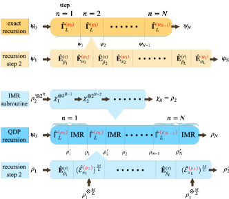
Figure 1: Illustration comparing exact and QDP implementation of nested fixed-point Grover search recursions. The top two rows describe the exact recursion. The uppermost row shows $N$ recursion steps by the unitary channel $\hat{\mathbf{\Gamma}}^{(\psi_{n-1})}_{L}$ containing $L$ memory-calls to the instruction state $\psi_{n-1}$. The resulting state of $n$th recursion step is $\psi_{n}$. The second row from the top gives a more detailed picture of each recursion step, where reflections around the fixed state $\hat{\mathbf{E}}^{(\tau)}_{\beta_{i}}$ are interlaced with memory-calls $\hat{\mathbf{E}}^{(\psi_{n-1})}_{\alpha_{i}}$. The bottom three rows represent the QDP implementation. The middle one among them outlines the overall protocol of $N$ recursions, where interferential mixedness reduction (IMR) protocols follow each dynamic implementation $\hat{\mathmybb{\Gamma}}^{(\rho_{n-1})}_{L}$ approximating $\hat{\mathbf{\Gamma}}^{(\rho_{n-1})}_{L}$. Note that the instruction state $\rho_{n-1}$ for each recursion is different from the exact instruction $\psi_{n-1}$ due to the inevitable error occurring from QDP implementation. In the lowermost row, it is shown that each memory-call $\hat{\mathbf{E}}^{(\psi_{n-1})}_{\alpha_{i}}$ is implemented by $\frac{M}{L}$ DME memory-usage queries consuming $\frac{M}{L}$ copies of the instruction state. The resulting state of the approximate channel $\hat{\mathmybb{\Gamma}}^{(\rho_{n-1})}_{L}$ is $\rho_{n}^{\prime}$, which is different from the next instructions state $\rho_{n}$. The next instruction state is prepared from $\rho_{n}^{\prime}$ using IMR protocols, described in the third row from the top. Each round of IMR protocol halves the number of copies one have, and total $R$ rounds are executed at each recursion step.

In this section, we delineate the entire protocol for the QDP implementation of nested fixed-point Grover search recursions. See Fig. 1 for the overall structure of the section. The exact recursion (two uppermost rows in the figure) is analyzed in Sec. IV.1 with the explicit formula giving the distance between the resulting state and the target state after each recursion. QDP implementation of the recursion is carried out by combining two subroutines: approximation of the recursion unitary using DME memory-usage queries (lowermost row in the figure) and the interferential mixedness reduction (IMR) subroutine (third row from the top) that maintains the mixedness of the instruction states below some threshold. Both of these subroutines are introduced in Sec. IV.2. In the rest of the section, we calculate the total cost of this implementation, namely the depth of the circuit and the number of copies needed, and show that the final state can be made arbitrarily close to the desired final state.

IV.1 Exact implementation of nested fixed-point Grover search

The analysis of the nested fixed-point Grover search, introduced in Ref. [11], involves Chebyshev polynomials of the first kind

$$T_{m}(x)=\begin{cases}\cos\bigl{(}m\arccos(x)\bigr{)},&\lvert x\rvert\leq 1\ ,\\ \cosh\bigl{(}m\operatorname{arcosh}(x)\bigr{)},&\lvert x\rvert>1\ .\end{cases}$$ (54)

We observe that if $\lvert x\rvert\leq 1$ then $\lvert T_{m}(x)\rvert\leq 1$ and $T_{l}(T_{m}(x))=T_{lm}(x)$ . Choosing $l=m^{-1}$ gives a special case

$$T_{m^{-1}}\left(T_{m}(x)\right)=T_{1}(x)=x,$$ (55)

and we will also use the property that $T_{m}(1)=1$.

We begin with $n=0$, which is to specify that we are given the initial state $|{\psi_{0}}\rangle$, and target state $|{\tau}\rangle$. In the $n$th step of the iteration, we apply a composite unitary operation with $L$ memory-calls

$$\hat{\Gamma}^{(\psi_{n-1})}_{L}=\hat{E}^{(\psi_{n-1})}_{\alpha_{L}}\hat{E}^{(\tau)}_{\beta_{L}}\cdots\hat{E}^{(\psi_{n-1})}_{\alpha_{1}}\hat{E}^{(\tau)}_{\beta_{1}}$$ (56)

to the iterated state $|{\psi_{n-1}}\rangle$ obtaining $|{\psi_{n}}\rangle=\hat{\Gamma}^{(\psi_{n-1})}_{L}|{\psi_{n-1}}\rangle$. The composite unitary operation in Eq. (56) consists of partial reflection unitaries defined as

$$\hat{E}^{(\psi)}_{s}=\mathmybb{1}-(1-e^{-is})|{\psi}\rangle\!\langle{\psi}|\ ,$$ (57)

with angle $s$, where we have adapted the notation $\psi=|{\psi}\rangle\!\langle{\psi}|$ and $\tau=|{\tau}\rangle\!\langle{\tau}|$ for pure states. When $s=\pi$, we obtain the usual reflection unitary around the state $|{\psi}\rangle$. In Eq. (56), following in the steps of  [11], we consider $L$ partial reflections around both $|{\tau}\rangle$ and $|{\psi_{n-1}}\rangle$ with angles

$$\alpha_{l}(q)=-\beta_{L-l+1}(q)=2\cot^{-1}\left(\tan\left(\frac{2\pi l}{2L+1}\right)\sqrt{1-\left[T_{1/(2L+1)}(q)\right]^{-2}}\right)\ ,$$ (58)

defined with some number $q$. The choice of the parameter $q$ determines the final distance to the target state as [11]

$$\frac{1}{2}\left\lVert\tau-\hat{\Gamma}^{(\psi)}_{L}(\psi)\left(\hat{\Gamma}^{(\psi)}_{L}\right)^{\dagger}\right\rVert_{1}=qT_{2L+1}\left(T_{1/(2L+1)}(q^{-1})\frac{1}{2}\lVert\tau-\psi\rVert_{1}\right)\ .$$ (59)

Lemma 10.

Suppose that the parameter $q$ in Eq. (58) is chosen to be $q=\delta_{n}$ for the recursion unitary $\hat{\Gamma}^{(\psi_{n-1})}_{L}$ at any $n$, where

$$\delta_{n}=\operatorname{sech}\left((2L+1)\operatorname{arcsech}\left(\delta_{n-1}\right)\right)\ ,\quad\forall n>0\ ,$$ (60)

starting from the base $\delta_{0}=\frac{1}{2}\lVert\tau-\psi_{0}\rVert_{1}$. Then $\frac{1}{2}\left\lVert\tau-\psi_{n}\right\rVert_{1}=\delta_{n}$ for all $n$, where $\psi_{n}$ is recursively defined as $|{\psi_{n}}\rangle=\hat{\Gamma}^{(\psi_{n-1})}_{L}|{\psi_{n-1}}\rangle$.

Proof.

We first observe that Eq. (60) is equivalent to

$$\delta_{n}^{-1}=T_{2L+1}\left(\delta_{n-1}^{-1}\right)\ ,$$ (61)

by recalling that ${\rm arcsech}(x)={\rm arcosh}(x^{-1})$. In particular, this also means that by applying $T_{1/(2L+1)}$ to both sides, we get

$$T_{1/(2L+1)}(\delta_{n}^{-1})=T_{1/(2L+1)}\left(T_{2L+1}\left(\delta_{n-1}^{-1}\right)\right)=\delta_{n-1}^{-1}.$$ (62)

We may now use this identity in simplifying the trace distance of interest: starting from the general relation Eq. (59) with $q=\delta_{n}$,

$$\frac{1}{2}\lVert\tau-\psi_{n}\rVert_{1}=\delta_{n}T_{2L+1}\left(T_{1/(2L+1)}\bigl{(}\delta_{n}^{-1}\bigr{)}\frac{1}{2}\lVert\tau-\psi_{n-1}\rVert_{1}\right)=\delta_{n}T_{2L+1}\left(\delta_{n-1}^{-1}\frac{1}{2}\lVert\tau-\psi_{n-1}\rVert_{1}\right)\ ,$$ (63)

where the second equality comes from applying Eqs. (62). If the Lemma is true for step $n-1$, i.e. if $\frac{1}{2}\lVert\tau-\psi_{n-1}\rVert_{1}=\delta_{n-1}$, then Eq. (63) leads to $\frac{1}{2}\lVert\tau-\psi_{n}\rVert_{1}=\delta_{n}$ using $T_{2L+1}(1)=1$. Since the base case $\frac{1}{2}\lVert\tau-\psi_{0}\rVert_{1}=\delta_{0}$ is true, the lemma holds by induction. ∎

The explicit form of the $\delta_{N}$, i.e. the distance to the target state after $N$ iterations can also be derived. From Eqs. (55) and (61), $\delta_{N}^{-1}=T_{(2L+1)^{N}}\left(\delta_{0}^{-1}\right)$, or equivalently,

$$\delta_{N}=\operatorname{sech}\left((2L+1)^{N}\operatorname{arcosh}\Bigl{(}\delta_{0}^{-1}\Bigr{)}\right)\ .$$ (64)

For large $N$, Eq. (64) asymptotically behaves as $\delta_{N}=\mathcal{O}\left(e^{-\operatorname{arcosh}\bigl{(}\delta_{0}^{-1}\bigr{)}(2L+1)^{N}}\right)\$. A typical setting of a Grover search starts from the initial fidelity $F_{0}=1-\delta_{0}^{2}\ll 1$, e.g. the initial state is a superposition of all basis states. Then the decay rate can be rewritten as

$$\operatorname{arcosh}\left(\delta_{0}^{-1}\right)=\operatorname{arcosh}((1-F_{0})^{-1/2})=\sqrt{F_{0}}+\mathcal{O}(F_{0}^{3/2})\ ,$$ (65)

by Taylor expansion. If only the leading order is taken, $\delta_{N}\sim e^{-\sqrt{F_{0}}(2L+1)^{N}}$, and thus

$$(2L+1)^{N}=\mathcal{O}\left(\log\left(\delta_{N}^{-1}\right)F_{0}^{-1/2}\right)$$ (66)

is needed for the final distance $\delta_{N}$. The circuit depth for the entire algorithm is proportional to Eq. (66) due to the unfolding implementation, and it contains the characteristic Grover scaling factor $F_{0}^{-1/2}$. If a non-recursive algorithm is applied, Eq. (64) can still be used with $N=1$. Denote the final distance as

$$\delta^{\prime}=\operatorname{sech}\left((2L^{\prime}+1)\operatorname{arcosh}\left(\delta_{0}^{-1}\right)\right),$$ (67)

when the alternation length of this algorithm is $L^{\prime}$. For $\delta^{\prime}=\delta_{N}$, the alternation length of the non-nested algorithm should satisfy $2L^{\prime}+1=(2L+1)^{N}$, resulting in exponentially many partial reflections. Note that Eq. (66) then implies $L^{\prime}\sim F_{0}^{-1/2}$, which displays the quantum advantage compared to the classical search requiring $L^{\prime}\sim F_{0}^{-1}$.

IV.2 Robustness of dynamic programming for the Grover search

In this section, we study the nested fixed-point Grover search algorithm implemented with bounded noise arising from using a dynamic programming approach. We establish the robustness of the algorithm against small implementation errors.

IV.2.1 Distance bounds after a DME implementation

In this subsection, we introduce the DME implementation of an iteration of the dynamic Grover search. We first establish (through Proposition 11 and Corollary 12) that the DME implementation still has the essential feature of the Grover search, namely all relevant states are effectively two-dimensional. Then the main results Lemma 14 and Corollary 15 provide the upper bound of a distance after one iteration of DME implemented Grover search, starting from a mixed state. In short, we observe that whenever the initially prepared state is close to being pure, then the distance to our Grover target state still follows a similar recursive relation as before, namely Eq. (83).

The ‘dynamic’ parts of the recursion unitary $\hat{\Gamma}^{(\rho)}_{L}$ are the memory-calls $\hat{E}^{(\rho)}_{\alpha}$, i.e. partial reflectors around the state $\rho$. Hence, DME (Def. 6) is the right choice of memory-usage query to use for implementing the memory-call $\hat{E}^{(\rho)}_{\alpha}$. To recap, the DME memory-usage query can be written as

$$\hat{\mathcal{E}}^{(\rho)}_{s}\left(\sigma\right)=\cos^{2}(s)\sigma-i\sin(s)\cos(s)[\rho,\sigma]+\sin^{2}(s)\rho\ ,$$ (68)

with the duration $s$ of our choice. If $M$ queries are made with $s=\frac{\alpha}{M}$, the implemented channel $(\hat{\mathcal{E}}^{(\rho)}_{s}(\sigma))^{M}$ approximates the memory-call $\hat{E}^{(\rho)}_{\alpha}$ with error $\mathcal{O}(1/M)$.

There are two key considerations in the implementation of quantum instructions via DME:

1. The implementation of a recursion step $\hat{\Gamma}^{(\psi)}_{L}$ becomes non-unitary even when the instruction state $\psi=|{\psi}\rangle\!\langle{\psi}|$ and the input state $\phi=|{\phi}\rangle\!\langle{\phi}|$ are pure. To see this, consider a special case of DME protocol with pure instruction state $\psi$ and input state $\phi$,

   $$\hat{\mathcal{E}}^{(\psi)}_{s}(\phi)=\cos^{2}(s)\phi+\sin^{2}(s)\psi-i\sin(s)\cos(s)\langle{\psi}|{\phi}\rangle|{\psi}\rangle\!\langle{\phi}|+\mathrm{h.c.}.$$ (69)

   We may directly compute the purity as

   $$\operatorname{Tr}\left[\left\{\hat{\mathcal{E}}^{(\psi)}_{s}(\phi)\right\}^{2}\right] =\cos^{4}(s)+\sin^{4}(s)+2\sin^{2}(s)\cos^{2}(s)\left(2\lvert\langle{\psi}|{\phi}\rangle\rvert^{2}-\lvert\langle{\psi}|{\phi}\rangle\rvert^{4}\right)$$ (70)

   $$=1-2\sin^{2}(s)\cos^{2}(s)\left(1-\lvert\langle{\psi}|{\phi}\rangle\rvert^{2}\right)^{2}\neq 1,$$

   hence $\rho_{n}$, the state after $n$ iterations of the Grover search recursion, is no longer pure in general.

2. Another important property to check is whether DME maps a target state supported on a two-dimensional subspace to another (now potentially mixed) state supported on the same space. In the exact algorithm, state vectors always stay in the space

   $$\mathcal{H}_{\rm rel}\coloneq\mathrm{span}\left\{|{\tau}\rangle,|{\tau^{\perp}}\rangle\coloneq\frac{|{\psi_{0}}\rangle-\langle{\tau}|{\psi_{0}}\rangle|{\tau}\rangle}{\sqrt{1-|\langle{\tau}|{\psi_{0}}\rangle|^{2}}}\right\},$$ (71)

   defined by the initial state vector $|{\psi_{0}}\rangle$ and the target state vector $|{\tau}\rangle$. This restriction is the reason that the fixed-point Grover search of [11] could utilize a $\mathrm{SU(2)}$ representation. To establish similar restriction for mixed states, we define

   $$\mathcal{S}_{\rm rel}\coloneq\left\{\rho\,|\,\rho:\text{density matrix},\ \mathrm{supp}(\rho)\subset\mathcal{H}_{\rm rel}\right\}$$ (72)

   the set of density matrices having support only in $\mathcal{H}_{\rm rel}$. Proposition 11 then rigorously shows that all relevant density operators resulting from the DME implementation stay in $\mathcal{S}_{\rm rel}$.

Proposition 11.

Suppose two states $\rho,\sigma\in\mathcal{S}_{\rm rel}$. The state after a DME channel $\sigma^{\prime}=\hat{\mathcal{E}}^{(\rho)}_{s}(\sigma)$ defined in Eq. (39) is also contained in $\mathcal{S}_{\rm rel}$. In other words, for all $s\in\mathbb{R}$, we have that $\hat{\mathcal{E}}^{(\mathcal{S}_{\mathrm{rel}})}_{s}(\mathcal{S}_{\mathrm{rel}})\subset\mathcal{S}_{\mathrm{rel}}\$.

Proof.

From direct calculation,

$$\hat{\mathcal{E}}^{(\rho)}_{s}(\sigma)|{\phi}\rangle=\cos^{2}(s)\sigma|{\phi}\rangle-i\sin(s)\cos(s)[\rho,\sigma]|{\phi}\rangle+\sin^{2}(s)\rho|{\phi}\rangle=0\ ,$$ (73)

whenever $|{\phi}\rangle\in\mathcal{H}_{\rm rel}^{\mathsf{C}}$. Therefore, $\mathrm{supp}(\hat{\mathcal{E}}^{(\rho)}_{s}(\sigma))\subset\mathcal{H}_{\rm rel}$. ∎

Noticing that DME for dynamic Grover iterations satisfies these conditions at every step of the recursion, we can be sure that the states generated by QDP in Grover search have full support in the relevant Hilbert space representation.

Corollary 12.

The QDP implementation of Grover search using DME generates a sequence of states $\rho_{n}\in\mathcal{S}_{\rm rel}$ for all $n\in\mathbb{N}$ whenever $\rho_{0}=\psi_{0}\in\mathcal{S}_{\rm rel}$.

Proof.

From Proposition 11, DME protocols map states in $\mathcal{S}_{\rm rel}$ to $\mathcal{S}_{\rm rel}$. Furthermore, reflections around the target state $\tau\in\mathcal{S}_{\rm rel}$, which is implemented by an exact unitary, not DME, also ensures that $\hat{\mathbf{E}}^{(\tau)}_{s}\left(\sigma\right)\in\mathcal{S}_{\rm rel}$ whenever $\sigma\in\mathcal{S}_{\rm rel}$. Since a recursion step of Grover search comprises the above two operations, the state after the iteration, $\rho_{n}$, also stays in $\mathcal{S}_{\rm rel}$. ∎

Corollary 12 enables a simple representation of intermediate states $\rho_{n}$. Defining the rank-$2$ projector onto $\mathcal{H}_{\rm rel}$, $\mathmybb{1}_{\rm rel}=|{\tau}\rangle\!\langle{\tau}|+|{\tau^{\perp}}\rangle\!\langle{\tau^{\perp}}|$, we note that this operator is invariant under an exact Grover recursion step with respect to any state $\phi\in\mathcal{S}_{\rm rel}$, i.e.

$$\hat{\mathbf{\Gamma}}^{(\phi)}_{L}\left(\mathmybb{1}_{\rm rel}\right)=\mathmybb{1}_{\rm rel},$$ (74)

due to unitarity of $\hat{\mathbf{\Gamma}}^{(\phi)}_{L}$. Since $\dim(\mathcal{H}_{\rm rel})=2$, we can decompose any $\rho\in\mathcal{S}_{\rm rel}$ in its eigenbasis

$$\rho=(1-a)|{\psi}\rangle\!\langle{\psi}|+a|{\psi^{\perp}}\rangle\!\langle{\psi^{\perp}}|=(1-x)|{\psi}\rangle\!\langle{\psi}|+x\frac{\mathmybb{1}_{\rm rel}}{2},$$ (75)

for $x=2a\in[0,1]$ by using the fact that $\mathmybb{1}_{\rm rel}=|{\psi}\rangle\!\langle{\psi}|+|{\psi^{\perp}}\rangle\!\langle{\psi^{\perp}}|$. We will refer to $\psi$ as the pure state associated with $\rho$ and $x$ as the mixedness parameter. Interestingly, the partial reflection around $\rho$ with angle $s$ can be rewritten using the observation that $[\psi,\mathmybb{1}_{\rm rel}]=0$:

$$\hat{E}^{(\rho)}_{s}=e^{-is\left[(1-x)\psi+x\frac{\mathmybb{1}_{\rm rel}}{2}\right]}=e^{-isx\frac{\mathmybb{1}_{\rm rel}}{2}}\hat{E}^{(\psi)}_{s(1-x)}\ ,$$ (76)

which is identical to the partial reflection around the corresponding pure state $\psi$ with the angle reduced by the factor $(1-x)$, apart from the phase factor globally acting on $\mathcal{H}_{\rm rel}$. If the mixedness parameter $x$ is known, one can effectively implement the reflection around the pure state $\psi$ using mixed states $\rho$ by adjusting the DME duration $s\mapsto s/(1-x)$.

Nevertheless, it is usually the case that only an upper bound, but not the exact amount of mixedness $x$ is known. The Proposition and the Lemma below assess the QDP implementation of a Grover search recursion step when the mixedness parameter $x$ is unknown. Instead of the exact partial reflection unitary channels $\hat{\mathbf{E}}^{(\psi)}_{s}=\hat{\mathbf{E}}^{(\rho)}_{s/(1-x)}$ around its associated pure state $\psi$, we employ DME queries $\hat{\mathcal{E}}^{(\rho)}_{s}$ as defined in Eq. (68).

Proposition 13.

Let $\rho=(1-x)\psi+x\frac{\mathmybb{1}_{\rm rel}}{2}$ be a state with an associated pure state $\psi$ and a mixedness parameter $x\in[0,\varepsilon]$ for some $0\leq\varepsilon<1$. A dynamic unitary channel

$$\hat{\mathbf{\Gamma}}^{(\rho)}_{L}=\hat{\mathbf{E}}^{(\rho)}_{\alpha_{L}}\circ\hat{\mathbf{E}}^{(\tau)}_{\beta_{L}}\circ\cdots\circ\hat{\mathbf{E}}^{(\rho)}_{\alpha_{1}}\circ\hat{\mathbf{E}}^{(\tau)}_{\beta_{1}}$$ (77)

that uses the same angles $\{\alpha_{l},\beta_{l}\}_{l}$ used in $\hat{\mathbf{\Gamma}}^{(\psi)}_{L}$ has the distance

$$\frac{1}{2}\left\lVert\hat{\mathbf{\Gamma}}^{(\psi)}_{L}-\hat{\mathbf{\Gamma}}^{(\rho)}_{L}\right\rVert_{\rm Tr}\leq\frac{L\pi\varepsilon}{2}\ ,$$ (78)

from the dynamic unitary channel constructed with the associated pure state $\psi$.

Proof.

First, observe that

$$\left\lVert\hat{\mathbf{\Gamma}}^{(\psi)}_{L}-\hat{\mathbf{\Gamma}}^{(\rho)}_{L}\right\rVert_{\rm Tr}\leq\sum_{i=1}^{L}\left\lVert\hat{\mathbf{E}}^{(\psi)}_{\alpha_{i}}-\hat{\mathbf{E}}^{(\rho)}_{\alpha_{i}}\right\rVert_{\rm Tr}\ ,$$ (79)

from the triangle inequality and the unitary invariance of the trace norm. The distance between $\hat{\mathbf{E}}^{(\rho)}_{\alpha}$ and $\hat{\mathbf{E}}^{(\psi)}_{\alpha}$ can be written as

$$\frac{1}{2}\left\lVert\hat{\mathbf{E}}^{(\psi)}_{\alpha}-\hat{\mathbf{E}}^{(\rho)}_{\alpha}\right\rVert_{\rm Tr}=\frac{1}{2}\max_{\sigma\in\mathcal{S}(\mathcal{H}_{\rm rel})}\left\lVert\hat{\mathbf{E}}^{(\psi)}_{\alpha}\left(\sigma\right)-\hat{\mathbf{E}}^{(\rho)}_{\alpha}(\sigma)\right\rVert_{1}=\frac{1}{2}\max_{\sigma\in\mathcal{S}(\mathcal{H}_{\rm rel})}\operatorname{Tr}\left\{\sqrt{\left(\hat{\mathbf{E}}^{(\psi)}_{\alpha}\left(\sigma\right)-\hat{\mathbf{E}}^{(\rho)}_{\alpha}(\sigma)\right)^{2}}\right\}\ .$$ (80)

Using the matrix notation

$$\psi=\begin{bmatrix}1&0\\ 0&0\end{bmatrix},\quad\rho=\begin{bmatrix}1-\frac{x}{2}&0\\ 0&\frac{x}{2}\end{bmatrix},\quad\sigma=\begin{bmatrix}p&q\\ q^{*}&1-p\end{bmatrix}\ ,$$ (81)

we arrive at the explicit expression

$$\left(\hat{\mathbf{E}}^{(\psi)}_{\alpha}(\sigma)-\hat{\mathbf{E}}^{(\rho)}_{\alpha}(\sigma)\right)^{2} =\begin{bmatrix}4\lvert q\rvert^{2}\sin^{2}\left(\frac{\alpha x}{2}\right)&0\\ 0&4\lvert q\rvert^{2}\sin^{2}\left(\frac{\alpha x}{2}\right)\end{bmatrix}\ .$$ (82)

The state $\sigma$ giving the maximum distance is the one having the maximal $\lvert q\rvert$. The condition that $\sigma\geq 0$ imposes $\lvert q\rvert\leq\frac{1}{2}$, and $\frac{1}{2}\lVert\hat{\mathbf{E}}^{(\psi)}_{\alpha}-\hat{\mathbf{E}}^{(\rho)}_{\alpha}\rVert_{\rm Tr}=\lvert\sin\left(\frac{\alpha x}{2}\right)\rvert$. From $\alpha\in[-\pi,\pi]$ and $\lvert\alpha\varepsilon\rvert<\pi$, we bound $\lvert\sin(\frac{\alpha x}{2})\rvert<\frac{\pi\varepsilon}{2}$ and achieve Eq. (78). ∎

Now we establish the main results of this subsection. We first define

$$\delta_{n}\coloneq\left(T_{(2L+1)}\left(\delta_{n-1}^{-1}\right)\right)^{-1}+\epsilon\ ,$$ (83)

and use it as the parameter $q=\delta_{n}$ when choosing angles Eq. (58). At the same time, we also demonstrate that $\delta_{n}$ bounds the distance to the target state, after an iteration of DME implementation with error $\epsilon$, i.e. it is the counterpart to Eq. (60) used for the exact iteration. Precise statements of this result are delineated in Lemma 14 and Corollary 15. Further analysis on Eq. (83) itself will be made in Sec. IV.3.

Lemma 14 (DME implementation subroutine).

We consider iteration $n$ of the nested Grover search algorithm. Assume that the initial state for the iteration $\rho_{n-1}=(1-x_{n-1})\psi_{n-1}+x_{n-1}\frac{\mathmybb{1}_{\rm rel}}{2}$ is unknown to us but satisfies the following:

• An associated pure state $\psi_{n-1}$ has the distance to the target state bounded by some number $\delta_{n-1}$, i.e. $\frac{1}{2}\lVert\tau-\psi_{n-1}\rVert_{1}\leq\delta_{n-1}$.

• The mixedness parameter is bounded by $x_{n-1}\leq\frac{\epsilon}{L\pi}$ for some number $\epsilon$.

Then, it is possible to prepare a state $\rho^{\prime}_{n}=(1-x_{n}^{\prime})\psi_{n}+x^{\prime}\frac{\mathmybb{1}_{\rm rel}}{2}$, such that

$$\frac{1}{2}\lVert\tau-\rho^{\prime}_{n}\rVert_{1} \leq\delta_{n}-\frac{\epsilon}{4},$$ (84)

where $\delta_{n}$ is defined in Eq. (83). The preparation requires consuming $\mathcal{O}(L^{2}\epsilon^{-1})$ copies of $\rho_{n-1}$.

Proof.

The preparation is performed by implementing nested fixed-point Grover search with DME memory-usage queries. Firstly, we choose the angles $\{\alpha_{l}(q),\beta_{l}(q)\}_{l}$ for the dynamic unitary $\hat{\mathbf{\Gamma}}^{(\psi_{n-1})}_{L}$. Following Lemma 10, we set $q=\operatorname{sech}((2L+1)\operatorname{arcsech}(\delta_{n-1}))$, or equivalently, $q=\delta_{n}-\epsilon$. Secondly, we denote the total number of DME queries $\hat{\mathcal{E}}^{(\rho_{n-1})}_{s}$ used for implementing $\hat{\mathbf{\Gamma}}^{(\psi_{n-1})}_{L}$ as $M$. Since $L$ memory-calls (partial reflections around $\rho_{n-1}$) are contained in $\hat{\mathbf{\Gamma}}^{(\psi_{n-1})}_{L}$, each memory-call employs $\frac{M}{L}$ DME memory-usage queries. The implemented channel reads

$$\hat{\mathmybb{\Gamma}}^{(\rho_{n-1})}_{L}\coloneq\left(\hat{\mathcal{E}}^{(\rho_{n-1})}_{s_{L}}\right)^{\frac{M}{L}}\circ\hat{\mathbf{E}}^{(\tau)}_{\beta_{L}}\circ\cdots\circ\left(\hat{\mathcal{E}}^{(\rho_{n-1})}_{s_{1}}\right)^{\frac{M}{L}}\circ\hat{\mathbf{E}}^{(\tau)}_{\beta_{1}}\ ,$$ (85)

with $s_{l}=\frac{\alpha_{l}L}{M}$, the angle $\alpha_{l}$ distributed equally to $\frac{M}{L}$ DME queries. The output state of the channel is

$$\rho^{\prime}_{n}:=\hat{\mathmybb{\Gamma}}^{(\rho_{n-1})}_{L}\left(\rho_{n-1}\right)=(1-x_{n}^{\prime})\psi_{n}+x_{n}^{\prime}\frac{\mathmybb{1}_{\rm rel}}{2}\ .$$ (86)

We additionally define the state after an exact unitary channel $\hat{\mathbf{\Gamma}}^{(\rho_{n-1})}_{L}$ as

$$\tilde{\rho}_{n}:=\hat{\mathbf{\Gamma}}^{(\rho_{n-1})}_{L}\left(\rho_{n-1}\right)=(1-x_{n-1})\phi_{n}+x_{n-1}\frac{\mathmybb{1}_{\rm rel}}{2}\ .$$ (87)

Since $\hat{\mathbf{\Gamma}}^{(\rho_{n-1})}_{L}$ is a unitary channel, it leaves the projector $\mathmybb{1}_{\rm rel}$ intact in Eq. (87), and the associated pure state

$$\phi_{n}=\hat{\mathbf{\Gamma}}^{(\rho_{n-1})}_{L}(\psi_{n-1})\ ,$$ (88)

while the mixedness parameter for $\tilde{\rho}_{n}$ is identical to that of $\rho_{n-1}$. We prove the Lemma starting from the triangle inequality $\lVert\tau-\rho^{\prime}_{n}\rVert_{1}\leq\lVert\tau-\phi_{n}\rVert_{1}+\lVert\phi_{n}-\rho^{\prime}_{n}\rVert_{1}$ and upper bounding each term in the RHS.

• Upper bound for $\lVert\tau-\phi_{n}\rVert_{1}$: Another triangle inequality gives

  $$\lVert\tau-\phi_{n}\rVert_{1}=\left\lVert\tau-\hat{\mathbf{\Gamma}}^{(\rho_{n-1})}_{L}(\psi_{n-1})\right\rVert_{1}\leq\left\lVert\tau-\hat{\mathbf{\Gamma}}^{(\psi_{n-1})}_{L}(\psi_{n-1})\right\rVert_{1}+\left\lVert\hat{\mathbf{\Gamma}}^{(\psi_{n-1})}_{L}(\psi_{n-1})-\hat{\mathbf{\Gamma}}^{(\rho_{n-1})}_{L}(\psi_{n-1})\right\rVert_{1}\ .$$ (89)

  The second term in the RHS is bounded by the trace norm distance of channels $\hat{\mathbf{\Gamma}}^{(\psi_{n-1})}_{L}$ and $\hat{\mathbf{\Gamma}}^{(\rho_{n-1})}_{L}$. Applying Proposition 13 and using the assumption $x_{n-1}\leq\frac{\epsilon}{L\pi}$,

  $$\left\lVert\hat{\mathbf{\Gamma}}^{(\psi_{n-1})}_{L}(\psi_{n-1})-\hat{\mathbf{\Gamma}}^{(\rho_{n-1})}_{L}(\psi_{n-1})\right\rVert_{1}\leq\left\lVert\hat{\mathbf{\Gamma}}^{(\psi_{n-1})}_{L}-\hat{\mathbf{\Gamma}}^{(\rho_{n-1})}_{L}\right\rVert_{\rm Tr}\leq\epsilon\ .$$ (90)

  The other term $\lVert\tau-\hat{\mathbf{\Gamma}}^{(\psi_{n-1})}_{L}(\psi_{n-1})\rVert_{1}$ resembles the final distance after an exact nested fixed-point Grover search in Lemma 10. However, we cannot directly apply Lemma 10, since we do not know the initial distance $\lVert\tau-\psi_{n-1}\rVert_{1}$ exactly; we only assume that it is bounded by $\delta_{n-1}$. Hence, we must start from the more general relation Eq. (59), which gives the equality

  $$\frac{1}{2}\left\lVert\tau-\hat{\mathbf{\Gamma}}^{(\psi_{n-1})}_{L}(\psi_{n-1})\right\rVert_{1}=(\delta_{n}-\epsilon)T_{2L+1}\left(T_{1/(2L+1)}\left((\delta_{n}-\epsilon)^{-1}\right)\frac{1}{2}\left\lVert\tau-\psi_{n-1}\right\rVert_{1}\right)\ ,$$ (91)

  substituting $q=\delta_{n}-\epsilon$. Recalling that $\delta_{n}-\epsilon=(T_{(2L+1)}(\delta_{n-1}^{-1}))^{-1}$ and Eq. (55), we get $T_{1/(2L+1)}((\delta_{n}-\epsilon)^{-1})=\delta_{n-1}^{-1}$. Eq. (91) then becomes

  $$\frac{1}{2}\left\lVert\tau-\hat{\mathbf{\Gamma}}^{(\psi_{n-1})}_{L}(\psi_{n-1})\right\rVert_{1}=(\delta_{n}-\epsilon)T_{2L+1}\left(\delta_{n-1}^{-1}\frac{1}{2}\left\lVert\tau-\psi_{n-1}\right\rVert_{1}\right)\ .$$ (92)

  Chebyshev polynomials follow $T_{2L+1}(x)\leq 1$ whenever $x\in[0,1]$, and the argument of $T_{2L+1}$ in the RHS, $\delta_{n-1}^{-1}\frac{1}{2}\lVert\tau-\psi_{n-1}\rVert_{1}$ is indeed smaller than or equal to $1$ from the assumption of the Lemma. Then $\frac{1}{2}\lVert\tau-\hat{\mathbf{\Gamma}}^{(\psi_{n-1})}_{L}(\psi_{n-1})\rVert_{1}\leq\delta_{n}-\epsilon$ follows, and we finally obtain the bound

  $$\frac{1}{2}\lVert\tau-\phi_{n}\rVert_{1}\leq\delta_{n}-\frac{\epsilon}{2}\ .$$ (93)

• Upper bound for $\lVert\phi_{n}-\rho^{\prime}_{n}\rVert_{1}$: Use the triangle inequality to obtain

  $$\lVert\phi_{n}-\rho^{\prime}_{n}\rVert_{1} \leq\left\lVert\phi_{n}-\hat{\mathmybb{\Gamma}}^{(\rho_{n-1})}_{L}(\psi_{n-1})\right\rVert_{1}+\left\lVert\hat{\mathmybb{\Gamma}}^{(\rho_{n-1})}_{L}(\psi_{n-1})-\rho^{\prime}_{n}\right\rVert_{1}$$

  $$=\left\lVert\hat{\mathbf{\Gamma}}^{(\rho_{n-1})}_{L}(\psi_{n-1})-\hat{\mathmybb{\Gamma}}^{(\rho_{n-1})}_{L}(\psi_{n-1})\right\rVert_{1}+\left\lVert\hat{\mathmybb{\Gamma}}^{(\rho_{n-1})}_{L}(\psi_{n-1})-\hat{\mathmybb{\Gamma}}^{(\rho_{n-1})}_{L}(\rho_{n-1})\right\rVert_{1}\ .$$ (94)

  The first term is bounded by

  $$\left\lVert\hat{\mathbf{\Gamma}}^{(\rho_{n-1})}_{L}(\psi_{n-1})-\hat{\mathmybb{\Gamma}}^{(\rho_{n-1})}_{L}(\psi_{n-1})\right\rVert_{1}\leq\left\lVert\hat{\mathbf{\Gamma}}^{(\rho_{n-1})}_{L}-\hat{\mathmybb{\Gamma}}^{(\rho_{n-1})}_{L}\right\rVert_{\rm Tr}\leq\sum_{l=1}^{L}\frac{M}{L}\left\lVert\hat{\mathbf{E}}^{(\rho_{n-1})}_{s_{l}}-\hat{\mathcal{E}}^{(\rho_{n-1})}_{s_{l}}\right\rVert_{\rm Tr}\ ,$$ (95)

  where the second inequality follows from comparing Eqs. (77) and (85). Making use of the explicit expressions in Eq. (81) again, the eigenvalues of $(\hat{\mathbf{E}}^{(\rho)}_{s}-\hat{\mathcal{E}}^{(\rho)}_{s})^{2}$ are evaulated to be degenerate and of order $\lambda=\mathcal{O}(s^{4})$. Numerical maximization over all possible values of $s_{l}$ and $\rho_{n-1}$ gives $\frac{1}{2}\lVert\hat{\mathbf{E}}^{(\rho_{n-1})}_{s_{l}}-\hat{\mathcal{E}}^{(\rho_{n-1})}_{s_{l}}\rVert_{\rm Tr}<0.71s_{l}^{2}$. Each $s_{l}$ can be bounded as $\lvert s_{l}\rvert=\lvert\frac{\alpha_{l}L}{M}\rvert\leq\frac{\pi L}{M}$, which leads to a bound

  $$\frac{1}{2}\left\lVert\hat{\mathbf{\Gamma}}^{(\rho_{n-1})}_{L}(\psi_{n-1})-\hat{\mathmybb{\Gamma}}^{(\rho_{n-1})}_{L}(\psi_{n-1})\right\rVert_{1}<\frac{7L^{2}}{M}\ .$$ (96)

  The second term of Eq. (• ‣ IV.2.1) is easier to bound; using data processing inequality,

  $$\frac{1}{2}\left\lVert\hat{\mathmybb{\Gamma}}^{(\rho_{n-1})}_{L}(\psi_{n-1})-\hat{\mathmybb{\Gamma}}^{(\rho_{n-1})}_{L}(\rho_{n-1})\right\rVert_{1}\leq\frac{1}{2}\lVert\psi_{n-1}-\rho_{n-1}\rVert_{1}=\frac{x_{n-1}}{2}\leq\frac{\epsilon}{2L\pi}\ .$$ (97)

  Therefore,

  $$\frac{1}{2}\lVert\phi_{n}-\rho^{\prime}_{n}\rVert_{1}<\frac{7L^{2}}{M}+\frac{\epsilon}{2L\pi}$$ (98)

Combining Eqs. (93) and (97), we achieve

$$\frac{1}{2}\lVert\tau-\rho^{\prime}_{n}\rVert_{1}<\delta_{n}-\frac{\epsilon}{2}+\frac{7L^{2}}{M}+\frac{\epsilon}{2L\pi}.$$ (99)

With $M=\mathcal{O}(L^{2}\epsilon^{-1})$, we can make

$$\frac{7L^{2}}{M}+\frac{\epsilon}{2L\pi}<\frac{\epsilon}{4}\ ,$$ (100)

which proves Eq. (84). The number of $\rho_{n-1}$ needed for the implementation is $M=\mathcal{O}(L^{2}\epsilon^{-1})$, which concludes the proof. ∎

Lemma 14 indicates that as long as the mixedness parameter stays low throughout the iterations, the total implementation error of the QDP Grover search can be kept bounded up to a desired accuracy. Although the mixedness parameter generally increases, we can bound the increment. Consider the distance $\frac{1}{2}\lVert\rho^{\prime}_{n}-\tilde{\rho}_{n}\rVert_{1}$: it is minimized when their associated pure states are identical, i.e.

$$\frac{1}{2}\lVert\rho^{\prime}_{n}-\tilde{\rho}_{n}\rVert_{1}\geq\frac{1}{2}\left\lVert(x^{\prime}_{n}-x_{n})\psi_{n}+(x_{n}-x^{\prime}_{n})\frac{\mathmybb{1}_{\rm rel}}{2}\right\rVert_{1}=\frac{\lvert x_{n}-x^{\prime}_{n}\rvert}{2}.$$ (101)

On the other hand,

$$\frac{1}{2}\lVert\rho^{\prime}_{n}-\tilde{\rho}_{n}\rVert_{1}\leq\frac{1}{2}\left\lVert\hat{\mathmybb{\Gamma}}^{(\rho_{n-1})}_{L}(\rho_{n-1})-\hat{\mathbf{\Gamma}}^{(\rho_{n-1})}_{L}(\rho_{n-1})\right\rVert_{\rm 1}\leq\frac{1}{2}\left\lVert\hat{\mathbf{\Gamma}}^{(\rho_{n-1})}_{L}-\hat{\mathmybb{\Gamma}}^{(\rho_{n-1})}_{L}\right\rVert_{\rm Tr}<\frac{7L^{2}}{M}\ .$$ (102)

Therefore,

$$0<x^{\prime}_{n}<x_{n-1}+\frac{7L^{2}}{M}<\frac{L\pi+2}{4L\pi}\epsilon\ ,$$ (103)

since we set $\frac{7L^{2}}{M}<\frac{L\pi-2}{4L\pi}\epsilon$ in Eq. (100).

In the next subsection, we describe a subroutine to reduce the mixedness factor $x^{\prime}_{n}$ into $x_{n}\leq\frac{\epsilon}{L\pi}$ so that we can continue the DME implementation without an accumulating error. However, if we eventually change the factor $x^{\prime}_{n}$, it is more important to get a bound for $\frac{1}{2}\lVert\tau-\psi_{n}\rVert_{1}$ corresponding to the associated pure state, rather than $\frac{1}{2}\lVert\tau-\rho^{\prime}_{n}\rVert_{1}$ as in Lemma 14.

Corollary 15.

The resulting state $\rho^{\prime}_{n}=(1-x_{n}^{\prime})\psi_{n}+x^{\prime}\frac{\mathmybb{1}_{\rm rel}}{2}$ of Lemma 14 has the associated pure state, such that

$$\frac{1}{2}\lVert\tau-\psi_{n}\rVert_{1} \leq\delta_{n}\ ,$$ (104)

where $\delta_{n}$ is defined in Eq. (83).

Proof.

The distance in Eq. (104) follows the triangle inequality $\lVert\tau-\psi_{n}\rVert_{1}\leq\lVert\tau-\rho^{\prime}_{n}\rVert_{1}+\lVert\rho^{\prime}_{n}-\psi_{n}\rVert_{1}$. The first term in the RHS is already bounded by $\delta_{n}-\frac{\epsilon}{4}$ in Lemma 14. The second term $\frac{1}{2}\lVert\rho^{\prime}_{n}-\psi_{n}\rVert_{1}=\frac{x^{\prime}_{n}}{2}$ by definition.

We then use Eq. (103) and obtain

$$\frac{1}{2}\lVert\rho^{\prime}_{n}-\psi_{n}\rVert_{1}<\frac{L\pi+2}{8L\pi}\epsilon\ .$$ (105)

Therefore, the final bound Eq. (104) can be established. ∎

IV.2.2 Mixedness reduction subroutine

In this section, we discuss a subroutine that allows us to keep the mixedness parameter $x_{n}$ low in any given step during the QDP protocol, which is the critical assumption in Lemma 14 and Corollary 15. The challenge here is that the mixedness parameter $x_{n}^{\prime}$, obtained after an iteration of QDP Grover recursion, increases from $x_{n-1}<\frac{\epsilon}{L\pi}$, whilst for the next iteration, we again need a state with mixedness parameter $x_{n}<\frac{\epsilon}{L\pi}$. Hence, we cannot directly use the state $\rho_{n}^{\prime}=\hat{\mathmybb{\Gamma}}^{(\rho_{n-1})}_{L}(\rho_{n-1})$ as an input for the next iteration.

In order to reduce $x^{\prime}_{n}$ to $x_{n}<\frac{\epsilon}{L\pi}$, we utilize a probabilistic protocol introduced in Ref. [21], which we will refer to as interferential mixedness reduction (IMR). In Lemma 16, we present the IMR protocol along with the proof, using notation that explicitly incorporates the mixedness parameter. Afterwards, in Proposition 17, we analyze the success probability of the mixedness reduction subroutine, which arises from using multiple IMR rounds.

Lemma 16 (Interferential mixedness reduction (IMR) [21]).

Let $\rho=(1-x)\psi+x\frac{\mathmybb{1}_{\rm rel}}{2}$ be a state in $\mathcal{S}_{\rm rel}$ with mixedness parameter $x\in[0,1)$. Using a controlled swap operation on the two copies of the state, i.e. $\rho^{\otimes 2}$, a purer state $\rho^{\prime}=(1-x^{\prime})\psi+x^{\prime}\frac{\mathmybb{1}_{\rm rel}}{2}$ with mixedness parameter $x^{\prime}=\frac{2+x}{4-2x+x^{2}}x\leq x$ can be prepared with success probability $(1-\frac{x}{2}+\frac{x^{2}}{4})$. This procedure is oblivious, i.e. no knowledge of the state $\psi$ or the subspace $\mathcal{H}_{\rm rel}$ is required.

Proof.

For completeness we provide a self-contained proof for this two-qubit protocol with details on symmetric subspace projection using an ancilla qubit. The presented proof adapts to our notation the original derivation found in the paragraph around Eq. (14) of Ref. [21]. We remark that Ref. [21] also contains better, yet more complicated, protocols using multiple copies of $\rho^{\otimes M}$ simultaneously.

Following [21], any two copies of a rank-2 state $\rho\in\mathcal{S}_{\rm rel}$ can be written as

$$\rho^{\otimes 2}=\frac{2x-x^{2}}{4}\Psi^{-}_{12}+\left(\frac{x^{2}}{4}\psi^{\perp}\otimes\psi^{\perp}+\frac{2x-x^{2}}{4}\Psi^{+}_{12}+\frac{(2-x)^{2}}{4}\psi\otimes\psi\right)\ ,$$ (106)

where $\psi^{\perp}\in\mathcal{S}_{\rm rel}$ is a pure state orthonormal to $\psi$ and $\Psi^{\pm}_{12}=|{\Psi^{\pm}}\rangle\!\langle{\Psi^{\pm}}|_{12}$ are Bell states, such that $|{\Psi^{\pm}}\rangle_{12}=\frac{1}{\sqrt{2}}(|{\psi\psi^{\perp}}\rangle_{12}\pm|{\psi^{\perp}\psi}\rangle_{12})$. Subscripts $1$ and $2$ denote the space each copy of $\rho$ lives in. The main protocol is to apply the projector $\frac{\mathmybb{1}_{12}+S_{12}}{2}$, where $\mathmybb{1}_{12}$ is the identity on the total space of two copies and $S_{12}$ is a swap between the first and the second copies. Note that

$$\frac{\mathmybb{1}_{12}+S_{12}}{2}=\psi^{\perp}\otimes\psi^{\perp}+\Psi^{+}_{12}+\psi\otimes\psi\ ,$$ (107)

after which $\Psi^{-}_{12}$ component will vanish from the state $\rho^{\otimes 2}$. This operation can be implemented by a linear combination of unitaries utilizing an additional ancilla qubit $|{0}\rangle_{A}$ [33], since both $\mathmybb{1}_{12}$ and $S_{12}$ are unitaries. To a state $|{0}\rangle\!\langle{0}|_{A}\otimes\rho^{\otimes 2}$ appended with ancilla, apply a unitary

$$U =\left(H_{A}\otimes\mathmybb{1}_{12}\right)\left(|{0}\rangle\!\langle{0}|_{A}\otimes\mathmybb{1}_{12}+|{1}\rangle\!\langle{1}|_{A}\otimes S_{12}\right)\left(H_{A}\otimes\mathmybb{1}_{12}\right)$$

$$=\left(|{0}\rangle\!\langle{0}|_{A}+|{1}\rangle\!\langle{1}|_{A}\right)\otimes\frac{\mathmybb{1}_{12}+S_{12}}{2}+\left(|{1}\rangle\!\langle{0}|_{A}+|{0}\rangle\!\langle{1}|_{A}\right)\otimes\frac{\mathmybb{1}_{12}-S_{12}}{2}\ ,$$ (108)

by concatenating Hadamard operators $H_{A}$ acting on the ancilla and a controlled swap operation, applying the swap $S_{12}$ between two copies conditioned on the ancilla state $|{1}\rangle$. After this operation, the ancilla plus system state becomes

$$U\left(|{0}\rangle\!\langle{0}|_{A}\otimes\rho^{\otimes 2}\right)U^{\dagger}= |{0}\rangle\!\langle{0}|_{A}\otimes\left(\frac{\mathmybb{1}_{12}+S_{12}}{2}\right)\rho^{\otimes 2}\left(\frac{\mathmybb{1}_{12}+S_{12}}{2}\right)+|{1}\rangle\!\langle{1}|_{A}\otimes\left(\frac{\mathmybb{1}_{12}-S_{12}}{2}\right)\rho^{\otimes 2}\left(\frac{\mathmybb{1}_{12}-S_{12}}{2}\right)$$

$$+\left[|{1}\rangle\!\langle{0}|_{A}\otimes\left(\frac{\mathmybb{1}_{12}-S_{12}}{2}\right)\rho^{\otimes 2}\left(\frac{\mathmybb{1}_{12}+S_{12}}{2}\right)+\mathrm{h.c.}\right]\ .$$ (109)

By measuring the ancilla in $\{|{0}\rangle_{A},|{1}\rangle_{A}\}$ basis, we effectively achieve (unnormalized) system states

$$\begin{cases}\frac{x^{2}}{4}\psi^{\perp}\otimes\psi^{\perp}+\frac{2x-x^{2}}{4}\Psi^{+}_{12}+\frac{(2-x)^{2}}{4}\psi\otimes\psi\ ,\quad&\text{if $|{0}\rangle_{A}$ is measured,}\\ \frac{2x-x^{2}}{4}\Psi^{-}_{12}\ ,\quad&\text{if $|{1}\rangle_{A}$ is measured,}\end{cases}$$ (110)

with probability given by their traces, $1-\frac{x}{2}+\frac{x^{2}}{4}$ and $\frac{2x-x^{2}}{4}$, respectively. For our purpose, the protocol is successful when $|{0}\rangle_{A}$ is measured, in which case the normalized density matrix

$$\Omega_{12}=\frac{4}{4-2x+x^{2}}\left(\frac{x^{2}}{4}\psi^{\perp}\otimes\psi^{\perp}+\frac{2x-x^{2}}{4}\Psi^{+}_{12}+\frac{(2-x)^{2}}{4}\psi\otimes\psi\right)$$ (111)

remains. The reduced state from $\Omega_{12}$ for both subsystems are the same and given as

$$\rho^{\prime}\coloneq\operatorname{Tr}_{1}\left[\Omega_{12}\right]=\operatorname{Tr}_{2}\left[\Omega_{12}\right]=(1-x^{\prime})\psi+x^{\prime}\frac{\mathmybb{1}_{\rm rel}}{2},$$ (112)

with $x^{\prime}=\frac{2+x}{4-2x+x^{2}}x<x$. The correlation between two subsystems in $\Omega_{12}$ might play a destructive role in our algorithm. Hence, we discard one of the copies and take only a single reduced state $\rho^{\prime}$. ∎

When $x\ll 1$, the success probability is close to $1$ and $x^{\prime}=\frac{x}{2}+\mathcal{O}(x^{2})$, i.e. we efficiently reduce the mixedness by just consuming copies of the same state, without changing the associated pure state $\psi$. Another potential merit of running IMR protocol is that we can estimate $x$ and thus $x^{\prime}$ by the success probability, which can be used to improve the process in Lemma 15 by modifying angles $\{s_{l}\}$ in $\hat{\mathcal{E}}^{(\rho)}_{s_{l}}$ according to the estimated value of mixedness parameter. Nevertheless, for simplicity of analysis, we restrict ourselves to the case where $x$ is completely unknown apart from its upper bound.

Lemma 17 (QDP mixedness reduction subroutine).

Let $\rho=(1-x)\psi+x\frac{\mathmybb{1}_{\rm rel}}{2}$ be a state in $\mathcal{S}_{\rm rel}$ with mixedness parameter $x\in[0,\varepsilon]$ for some $0\leq\varepsilon<\frac{1}{2}$. Given any maximum tolerable probability of failure $q_{\mathrm{th}}\geq 0$, one can choose any parameter $\mathsf{g}\in\mathbb{R}$ and prepare $M$ copies of $\rho^{\prime}=(1-x^{\prime})\psi+x^{\prime}\frac{\mathmybb{1}_{\rm rel}}{2}$, such that:

1. $x^{\prime}\in[0,\frac{\varepsilon}{\mathsf{g}}]$,

2. a number of $R=\mathcal{O}(\log(\mathsf{g}))$ IMR rounds in Lemma 16 is used,

3. a total of $M\times(\frac{2}{c})^{R}$ copies of $\rho$ is consumed, with $c\in(0,1)$ satisfying

   $$c=1-\frac{\varepsilon}{2}-M^{-\frac{1}{2}}\sqrt{\log\left(\frac{R}{q_{\rm th}}\right)}\ ,$$ (113)

4. the success probability of the entire subroutine is $q_{\rm succ}\geq 1-q_{\rm th}$.

Note that $M$ must be sufficiently large to guarantee $c>0$.

Proof.

To prove this lemma, we analyze $R$ sequential rounds of the IMR protocol, with initial and final states $\rho$ and $\rho^{\prime}$. Let us denote the intermediate states generated via the IMR protocols as $\{\chi_{j}\}_{j=0}^{R}$, where $\chi_{0}=\rho$ and $\chi_{R}=\rho^{\prime}$; and let $\{y_{j}\}_{j=0}^{R}$ be the corresponding mixedness parameter for each $\chi_{j}$ with $y_{0}=x$ and $y_{R}=x^{\prime}$. Furthermore, let us denote $M_{j}$ to be the number of copies of an intermediate state $\chi_{j}$ generated; hence, we obtain $M_{R}=M$ copies of the desired state $\rho^{\prime}$ at the end, and aim to show that $M_{0}=M\times(\frac{2}{c})^{R}$ suffices.

From Lemma 16, the mixedness parameter after $j$ rounds of the IMR protocol becomes

$$y_{j}=\frac{2+y_{j-1}}{4-2y_{j-1}+y_{j-1}^{2}}y_{j-1}\leq\left(\frac{1}{2}+\dfrac{3y_{j-1}}{5}\right)y_{j-1}\ ,$$ (114)

where the last inequality is obtained by comparing derivatives of the LHS and the RHS. The number of rounds $R$ is determined by the rate of mixedness reduction we desire. The final reduction $\frac{x^{\prime}}{x}=\frac{y_{R}}{y_{0}}\leq\mathsf{g}^{-1}$ is achievable if

$$\frac{y_{R}}{y_{0}}=\prod_{j=1}^{R}\frac{y_{j}}{y_{j-1}}\leq\prod_{j=1}^{R}\left(\frac{1}{2}+\dfrac{3y_{j-1}}{5}\right)\leq\left(\frac{1}{2}+\frac{3\varepsilon}{5}\right)^{R}\leq\mathsf{g}^{-1}\ ,$$ (115)

since $y_{j}\leq\varepsilon$ for all $j$. Therefore, $R=\mathcal{O}\left(\log(\mathsf{g})\right)$ is sufficient as claimed – note that $\log\left(\frac{1}{2}+\frac{3\varepsilon}{5}\right)$ to be $\mathcal{O}(1)$ since $\varepsilon<\frac{1}{2}$.

The parameter $c$ in the statement of the lemma can be interpreted as the ‘survival rate’ after each round of the IMR protocol. More specifically, the $j$-th round of the protocol is successful if at least $\frac{c}{2}M_{j-1}$ output states $\chi_{j}$ is prepared from $M_{j-1}$ copies of $\chi_{j-1}$. If successful, we discard all the surplus output copies and set $M_{j}=\frac{c}{2}M_{j-1}$. If not, we declare that the whole subroutine has failed. Hence, if the entire subroutine succeeds, the final number of copies $M=M_{R}$ is related to the initial number of copies as $M_{0}=(2/c)^{R}M$.

Finally, we estimate the success probability $q_{\rm succ}$ given $R,M,c,x$ and require it to be lower bounded with $(1-q_{\rm th})$. The failure probability of each round will be bounded using Hoeffding’s inequality. From Lemma 16, the success probability of preparing one copy of $\chi_{j}$ from a pair $\chi_{j-1}^{\otimes 2}$ is

$$p(y_{j-1})=1-\frac{y_{j-1}}{2}+\frac{y_{j-1}^{2}}{4}\geq 1-\frac{y_{j-1}}{2}\ .$$ (116)

At each round, $\frac{M_{j-1}}{2}$ independent trials of this IMR protocol are conducted. The probability of more than $c\frac{M_{j-1}}{2}$ attempts succeeds, i.e. the success probability of a round, is

$$q_{r}^{(j)}=1-F\left(\left\lceil\frac{cM_{j-1}}{2}-1\right\rceil;\frac{M_{j-1}}{2},p(y_{j-1})\right)\geq 1-F\left(\frac{cM_{j-1}}{2};\frac{M_{j-1}}{2},1-\frac{y_{j-1}}{2}\right)\ ,$$ (117)

where $F(k;n,q)$ is the cumulative binomial distribution function defined as

$$F(cn;n,p)=\sum_{i=0}^{\lfloor cn\rfloor}\binom{n}{i}p^{i}(1-p)^{n-i}\ .$$ (118)

Furthermore, the Hoeffding’s inequality gives $F(cn;n,p)\leq e^{-2n(p-c)^{2}}$, and consequently sets the bound

$$q_{r}^{(j)}\geq 1-e^{-M_{j}\left(1-\frac{y_{j-1}}{2}-c\right)^{2}}\ .$$ (119)

The success probability of an entire subroutine can then be bounded as

$$q_{\rm succ} =\prod_{j=1}^{R}q_{r}^{(j)}\geq\prod_{j=1}^{R}\left(1-e^{-M_{j}\left(1-\frac{y_{j-1}}{2}-c\right)^{2}}\right)>1-\sum_{j=1}^{R}e^{-M_{j}\left(1-\frac{y_{j-1}}{2}-c\right)^{2}}\ ,$$ (120)

where the last inequality uses $\prod_{j}(1-q_{j})>1-\sum_{j}q_{j}$ that holds when $q_{j}\in(0,1)$ for all $j$. Moreover, by recalling $\varepsilon\geq y_{j-1}$ and $M\leq M_{j}$ for all $j$, the final bound

$$q_{\rm succ}>1-Re^{-M\left(1-\frac{\varepsilon}{2}-c\right)^{2}}$$ (121)

is obtained. The prescribed failure threshold $q_{\rm th}$ holds when $e^{-M\left(1-\frac{\varepsilon}{2}-c\right)^{2}}=\frac{q_{\rm th}}{R}$ , or equivalently, when $M$ is sufficently large and Eq. (113) is true. ∎

Note that the upper bound for $c$ in Eq. (113) increases monotonically as $M$ increases. Hence, the process is more efficient in earlier iterations of the Grover recursion, when $M$, the number of output states required, is larger. The worst bound is achieved at the last iteration. Ideally, we want $M=1$ at the last iteration, since the goal of the Grover search algorithm is to prepare a single copy of the state $\rho_{N}$ close to the target state. However, the threshold failure probability $q_{\rm th}$ cannot be arbitrarily small in such case, even if $c=0$. To guarantee an arbitrarily small failure probability, we prepare redundant copies of $\rho_{N}$ and denote the number of these copies as $M_{r}$. If we allow the redundancy $M_{r}>1$, it is also possible to fix $c$ to be a constant. From now on, let us fix

$$c=1-\frac{\varepsilon}{2}-M_{r}^{-\frac{1}{2}}\sqrt{\log\left(\frac{R}{q_{\rm th}}\right)}=\frac{2}{3}\ ,$$ (122)

which can be achieved by modulating $M_{r}$ since $1-\frac{\varepsilon}{2}>\frac{3}{4}$.

In addition, we find $R=\mathcal{O}(\log(\mathsf{g}))$ by setting $\mathsf{g}$. In Eq. (103), the mixedness of $\rho^{\prime}_{n}$ is bounded by $\frac{L\pi+2}{4L\pi}\epsilon$, while we want a state $\rho_{n}$ whose mixedness parameter is reduced to $\frac{\epsilon}{L\pi}$. Hence, the reduction by the factor $\mathsf{g}=\frac{L\pi+2}{4}$ is needed and therefore $R=\mathcal{O}(\log(L))$. Combining all this, Eq. (122) gives the redundancy

$$M_{r}=\left(\frac{1}{3}-\frac{\varepsilon}{2}\right)^{-2}\log\left(\frac{\log(L)}{q_{\rm th}}\right)=\mathcal{O}\left(\log\left(\frac{1}{q_{\rm th}}\right)\right)\ ,$$ (123)

assuming that the subroutine succeeds almost surely, i.e. $q_{\rm th}\lesssim\frac{1}{\log(L)}$.

We assumed that $\varepsilon<\frac{1}{2}$ in Lemma 17, but this is always true for our algorithm. $\varepsilon$ is given as the mixedness parameter of $\rho^{\prime}_{n}$ after a DME implementation Lemma 14, which is bounded by $\frac{L\pi+2}{4L\pi}\epsilon<0.41\epsilon<\frac{1}{2}$, since $\epsilon<1$.

IV.3 QDP Grover search with linear circuit depth and exponential circuit width

In this subsection, we combine the results from Section IV.2 to prove a lemma describing a full QDP nested fixed-point Grover search algorithm.

Lemma 18 (QDP Grover search).

Consider the nested fixed-point Grover search with $N$ recursions and $2L$ partial reflections at each recursion step, and let

• $\tau=|{\tau}\rangle\!\langle{\tau}|$ be the target state of the search,

• $\psi_{0}=|{\psi_{0}}\rangle\!\langle{\psi_{0}}|$ be the initial state whose distance to the target $\frac{1}{2}\lVert\tau-\psi_{0}\rVert_{1}\eqcolon\delta_{0}$,

• $\epsilon\in(0,1)$ be the threshold implementation error parameter,

• $p_{\mathrm{th}}\lesssim\frac{N}{\log(L)}$ be the threshold failure probability of the algorithm.

Then, the QDP implementation of the search prepares the final state $\rho_{N}$ with

• the distance to the target state $\frac{1}{2}\lVert\tau-\rho_{N}\rVert_{1}\leq\delta_{N}+\frac{\epsilon}{2L\pi}$, where $\delta_{N}$ is defined recursively for any $n>0$ as

  $$\delta_{n}=\operatorname{sech}\left((2L+1)\operatorname{arcsech}\left(\delta_{n-1}\right)\right)+\epsilon,$$ (124)

• the success probability greater than $1-p_{\mathrm{th}}$,

• a circuit of depth $\mathcal{O}(L^{2}N\epsilon^{-1})$, and

• a number of initial state $\psi_{0}$ scaling as $L^{\mathcal{O}(N)}\epsilon^{-N}\log(p_{\rm th}^{-1})$.

In contrast, the unfolding implementation of the nested fixed-point Grover search has a circuit depth $\mathcal{O}((2L)^{N})$ and a constant width.

Proof.

The algorithm consists of $N$ iterations of the recursion step, where each iteration involves two subroutines: a DME implementation in Lemma 14 followed by a mixedness reduction subroutine in Proposition 17.

1. At a DME implementation subroutine, $\mathtt{I}_{n}$ copies of $\rho_{n-1}$ are transformed to $\mathtt{O}_{n}$ copies of $\rho_{n}^{\prime}$ deterministically. Input state

   $$\rho_{n-1}=(1-x_{n-1})\psi_{n-1}+x_{n-1}\frac{\mathmybb{1}_{\rm rel}}{2}\$$ (125)

   is assumed to satisfy $x_{n-1}<\frac{\epsilon}{L\pi}$ and $\frac{1}{2}\lVert\tau-\psi_{n-1}\rVert_{1}\leq\delta_{n-1}$, while the output state

   $$\rho_{n}^{\prime}=\hat{\mathmybb{\Gamma}}^{(\rho_{n-1})}_{L}(\rho_{n-1})=(1-x_{n}^{\prime})\psi_{n}+x_{n}^{\prime}\frac{\mathmybb{1}_{\rm rel}}{2}\ ,$$ (126)

   satisfies $x^{\prime}_{n}<\frac{L\pi+2}{4L\pi}\epsilon$ from Eq. (103), and $\lVert\tau-\psi_{n}\rVert_{1}\leq\delta_{n}$ by Corollary 15. For each channel $\hat{\mathmybb{\Gamma}}^{(\rho_{n-1})}_{L}$ implementation, $\mathcal{O}(L^{2}\epsilon^{-1})$ DME queries are made and consequently $\mathcal{O}(L^{2}\epsilon^{-1})$ copies of $\rho_{n-1}$ are consumed. Plus, $L$ partial reflections $\hat{\mathbf{E}}^{(\tau)}_{s}$ around the target state are also applied. In sum, we need

   $$\mathtt{I}_{n}=\mathcal{O}\left(\frac{L^{2}}{\epsilon}\right)\mathtt{O}_{n}$$ (127)

   copies of $\rho_{n-1}$ with depth $\mathcal{O}(\frac{L^{2}}{\epsilon})$ elementary gates for the subroutine.

2. At a mixedness reduction subroutine, described in Lemma 17, $\mathtt{O}_{n}$ copies of $\rho_{n}^{\prime}$, output from the DME implementation subroutine (Eq. (126)), are transformed into $\mathtt{I}_{n+1}$ copies of $\rho_{n}=(1-x_{n})\psi_{n}+x_{n}\frac{\mathmybb{1}_{\rm rel}}{2}$, such that $x_{n}<\frac{\epsilon}{L\pi}$, with a guarantee that the success probability $q_{\rm succ}$ is higher than $1-q_{\rm th}$ for some threshold value $q_{\rm th}$. The probability of $N$ such probabilistic subroutines to be all successful is

   $$p_{\rm succ}=q_{\rm succ}^{N}\geq\left(1-q_{\rm th}\right)^{N}\geq 1-Nq_{\rm th}\ ,$$ (128)

   where the second inequality follows from the Taylor expansion. Thus setting $q_{\rm th}=\frac{p_{\rm th}}{N}$ ensures that $p_{\rm succ}\geq 1-p_{\rm th}$ as required. Lemma 17 states $\mathtt{O}_{n}=\left(\frac{2}{c}\right)^{R}\mathtt{I}_{n+1}$ is needed, where $R$ is the number of IMR protocol rounds proportional to the $\log$ of rate of reduction $\frac{x_{n}^{\prime}}{x_{n}}$, while $c$ is the factor that decides how many transformed states survive after a round of the IMR protocol. As discussed in Eq. (122) and the following paragraph, we set $c=\frac{2}{3}$ and $R=\mathcal{O}(\log(L))$. Combining all,

   $$\mathtt{O}_{n}=3^{\mathcal{O}\left(\log(L)\right)}\mathtt{I}_{n+1}=\mathrm{poly}(L)\mathtt{I}_{n+1}\ ,$$ (129)

   and circuit depth $\mathcal{O}(R)=\mathcal{O}(\log(L))$ from $R$ repititions of interferential mixedness reduction protocols (Lemma 16) is added.

Finally, we account for the redundancy of the final number of copies $M_{r}$ in Eq. (123), introduced to guarantee high success probability. In other words, we set $I_{N}=M_{r}=\mathcal{O}(\log(Np_{\rm th}^{-1}))$. Then the initial number of copies needed

$$I_{0}=L^{\mathcal{O}(N)}\epsilon^{-N}\log(p_{\rm th}^{-1})$$ (130)

which is exponential in $N$. Furthermore, the circuit depth scales as

$$\mathcal{O}\left(\log(L)+\frac{L^{2}}{\epsilon}\right)N=\mathcal{O}\left(\frac{NL^{2}}{\epsilon}\right)\ ,$$ (131)

which is linear in $N$. ∎

IV.4 From Lemma 18 to Theorem 21

In Lemma 18, we have shown that the distance $\delta_{n}$ between the final state and the target state $\tau$ after $n$ QDP Grover search iterations follows the recursion relation Eq. (124). In this subsection, we demonstrate that for a reasonably small implementation error $\epsilon$, the sequence $\delta_{n}$ does not deviate from the sequence of distance obtained from ideal, errorless iterations. To do this, we set $\delta_{n+1}=h(\delta_{n})+\epsilon$, with the function

$$h(x)=\operatorname{sech}\left((2L+1)\operatorname{arcsech}(x)\right)\ .$$ (132)

Note that Eq. (132) gives distance recurrence relations for the exact nested fixed-point Grover search (Lemma 10), i.e. $\frac{1}{2}\lVert\tau-\psi_{n}\rVert_{1}=h(\frac{1}{2}\lVert\tau-\psi_{n-1}\rVert_{1})$ for $|{\psi_{n}}\rangle=\hat{\mathbf{\Gamma}}^{(\psi_{n-1})}_{L}|{\psi_{n-1}}\rangle$. By finding the range for fast spectral convergence (Def. 8), i.e. the range where its derivative $h^{\prime}(x)<r$ for some $r<1$ and $h(x)+\varepsilon<x$, we demonstrate that the resulting distance from $N$ iterations of the QDP implementation $\delta_{N}$ can still be arbitrarily close to that of the exact implementation.

As a first step, we establish the convexity of $h(x)$ in the range $x\in(0,1)$.

Proposition 19.

The function $h(x)$ defined as in Eq. (132) is monotonically increasing and convex in the range $x\in(0,1)$.

Proof.

Let us define $\tilde{L}\coloneq 2L+1$ for simplicity. The derivatives of $h(x)$ become

$$h^{\prime}(x) \coloneq\frac{dh(x)}{dx}=\frac{\tilde{L}\operatorname{sech}\left(\tilde{L}\operatorname{arcsech}(x)\right)\tanh\left(\tilde{L}\operatorname{arcsech}(x)\right)}{x\sqrt{1-x^{2}}}>0\ ,$$ (133)

from which the monotonicity of $h(x)$ follows. We define another variable $y\coloneq\operatorname{arcsech}\left(x\right)\in(0,\infty)$ and

$$g(y)\coloneq\frac{\tilde{L}\operatorname{sech}\left(\tilde{L}y\right)\tanh\left(\tilde{L}y\right)}{\operatorname{sech}(y)\tanh(y)}\ ,$$ (134)

satisfying $g(\operatorname{arcsech}(x))=h^{\prime}(x)$. Thus,

$$h^{\prime\prime}(x)\coloneq\frac{d^{2}h(x)}{dx^{2}}=\frac{dg(y)}{dy}\frac{dy}{dx}=-\frac{g^{\prime}(y)}{x\sqrt{1-x^{2}}}\ ,$$ (135)

and $h(x)$ is convex when $g^{\prime}(y)\coloneq\frac{dg(y)}{dy}$ is negative for $y>0$. From direct calculation

$$g^{\prime}(y)=\frac{\tilde{L}}{y}\frac{\cosh^{2}(y)\sinh(\tilde{L}y)}{\sinh(y)\cosh^{2}(\tilde{L}y)}\left[\tilde{L}y\frac{2\operatorname{sech}^{2}(\tilde{L}y)-1}{\tanh(\tilde{L}y)}-y\frac{2\operatorname{sech}^{2}(y)-1}{\tanh(y)}\right]\ .$$ (136)

Note that the sign of $g^{\prime}(y)$ is determined by terms inside the square bracket, which can be written as $f(\tilde{L}y)-f(y)$ by defining

$$f(y)\coloneq y\frac{2\operatorname{sech}^{2}(y)-1}{\tanh(y)}\ .$$ (137)

$f(y)$ is a monotonically decreasing function, hence $f(\tilde{L}y)-f(y)<0$ and $h(x)$ is convex. ∎

Due to convexity, $h^{\prime}(x)<r$ can be guaranteed whenever $x<\delta^{*}$ such that $h^{\prime}(\delta^{*})=r$. The threshold $\delta^{*}$ is the smallest when $L=1$ and grows as $L$ increases. Setting $L=1$, we numerically obtain that $\delta^{*}=0.73$ is sufficient for $h^{\prime}(x)<1$ for any $L$. With a more reasonable choice $L=5$, the threshold becomes $\delta^{*}\simeq 0.93$. Furthermore, Proposition 19 also implies that when $\epsilon$ is small, $h(x)+\epsilon=x$ has two solutions $x_{1}$ and $x_{2}$ with $x_{1}<x_{2}$ in the range $x\in(0,1)$.

Assuming $\epsilon\ll 1$, we can evaluate the approximate value of $x_{1}$ and $x_{2}$.

Proposition 20.

When $\epsilon\ll 1$, a larger solution $x_{2}$ satisfying $h(x)+\epsilon=x$ is

$$x_{2}=1-\frac{1}{4(L^{2}+L)}\epsilon+\mathcal{O}(\epsilon^{2})\ .$$ (138)

Proof.

The equation $h(x)+\epsilon=x$ can be rewritten as $\tilde{L}\operatorname{arcsech}(x)=\operatorname{arcsech}(x-\epsilon)$. Let us define $y\coloneq 1-x$ and assume that $y$ and $\epsilon$ are both small. The equation becomes

$$\tilde{L}\sqrt{2y}=\sqrt{2(y+\epsilon)}+\mathcal{O}(y^{3/2})\$$ (139)

or $y=\frac{1}{\tilde{L}^{2}-1}\epsilon+\mathcal{O}(\epsilon^{2})$, which proves the proposition. ∎

Proposition 20 indicates that for any reasonably small $\epsilon$, we have $\delta^{*}<x_{2}$. Hence, for the fast spectral convergence of the recursion, we only need to ensure that the initial distance $\delta_{0}<\delta^{*}$. Now we demonstrate that the QDP implementation of the Grover search can converge to the exact algorithm with an arbitrary error $\eta>0$.

Theorem 21 (Efficient QDP Grover search algorithm).

Consider the nested fixed-point Grover search with $N$ recursions and $2L$ partial reflections at each recursion step. Furthermore, assume that the distance between the initial state $\psi_{0}$ and the target state $\tau$ satisfies $\frac{1}{2}\lVert\tau-\psi_{0}\rVert_{1}\eqcolon\delta_{0}<\delta^{*}$, where $\delta^{*}$ is determined by $h^{\prime}(\delta^{*})=1$ with $h^{\prime}$ defined in Eq. (133). Then, QDP implementation of the algorithm can output a state $\rho_{N}$, whose distance to the target state $\tau$ is arbitrarily close to that of the $|{\psi_{N}}\rangle$, an output from the exact algorithm, i.e.

$$\frac{1}{2}\lVert\tau-\rho_{N}\rVert_{1}\leq\frac{1}{2}\lVert\tau-\psi_{N}\rVert_{1}+\eta\ ,$$ (140)

for any $\eta>0$. In addition, the success probability of the QDP implementation exceeds $1-p_{\mathrm{th}}$ for any $p_{\mathrm{th}}<\frac{N}{\log(L)}$. This implementation requires $L^{\mathcal{O}(N)}\eta^{-N}\log(p_{\rm th}^{-1})$ copies of $|{\psi_{0}}\rangle$ and a circuit of depth $\mathcal{O}(L^{2}N\eta^{-1})$.

Proof.

After $N$ iterations of the exact algorithm, output state $\psi_{N}$ satisfies

$$\frac{1}{2}\lVert\tau-\psi_{N}\rVert_{1}=\tilde{\delta}_{N},\quad\frac{1}{2}\lVert\tau-\psi_{0}\rVert_{1}=\delta_{0}\ ,$$ (141)

where $\tilde{\delta}_{N}$ is recursively defined by $\tilde{\delta}_{n+1}=h(\tilde{\delta}_{n})$ and $\tilde{\delta}_{0}=\delta_{0}$. On the other hand, the QDP implementation (Lemma 18) gives

$$\frac{1}{2}\lVert\tau-\rho_{N}\rVert_{1}\leq\delta_{N}+\frac{\epsilon}{2L\pi}\ ,$$ (142)

by using $L^{\mathcal{O}(N)}\epsilon^{-N}\log(p_{\rm th}^{-1})$ copies of the initial state $\psi_{0}$, where $\delta_{n+1}=h(\delta_{n})+\epsilon$ and $\epsilon$ is the parameter that decides circuit depth and width of the QDP algorithm.

Since $\delta_{0}<\delta^{*}$, we have $h^{\prime}(\delta_{0})<r$ for some $r<1$ and $h(\delta_{0})+\epsilon<\delta_{0}$. Then $\delta_{1}=h(\delta_{0})+\epsilon$ and $\delta_{2}=h(h(\delta_{0})+\epsilon)+\epsilon<h^{2}(\delta_{0})+(r+1)\epsilon$. Hence, we can bound $\delta_{N}$ by

$$\delta_{N}<h^{N}(\delta_{0})+\sum_{n=0}^{N-1}r^{n}\epsilon=\tilde{\delta}_{N}+\frac{1-r^{N}}{1-r}\epsilon\ .$$ (143)

Setting $\epsilon=\mathcal{O}(\eta)$, we achieve $\frac{1}{2}\lVert\tau-\rho_{N}\rVert_{1}\leq\tilde{\delta}_{N}+\eta$. In other words, by using circuit depth linear in $\eta$ and width exponential in $\eta$, QDP algorithm converges to the exact algorithm with error bounded by an arbitrary number $\eta>0$. ∎

In the unfolding implementation, the circuit depth scales as $(2L+1)^{N}\sim\log(\delta_{N}^{-1})(1-\delta_{0}^{2})^{-1/2}$ with the Grover scaling factor $(1-\delta_{0}^{2})^{-1/2}$. However, for sampling-based Grover search algorithms, i.e. if copies of the initial state $\psi_{0}$ are used instead of the oracle $\hat{E}^{(\psi_{0})}_{\alpha}$, Ref. [14] proved that at least $\mathcal{O}(L^{2N})=\mathcal{O}((1-\delta_{0}^{2})^{-1})$ copies of the initial state are needed. The QDP implementation also obeys this scaling and the number of copies in Thm. 21 must scale faster than $\mathcal{O}(L^{2N})$.

V Oblivious Schmidt decomposition using double-bracket iterations

Oblivious Schmidt decomposition (OSD) is done by diagonalizing a reduced state $\rho_{0}^{(A)}=\operatorname{Tr}_{B}[\psi_{0}]$ of the given entangled state $\psi_{0}$, without learning the state itself. For diagonalization, we use a recently-proposed quantum algorithm [12], which we call double-bracket iterations, that adapts the continuous gradient flow for matrices for discrete gate-based quantum computing models.

V.1 Double-bracket recursions

In this section, we expound on the double-bracket iteration algorithm, which can be used for scenarios beyond OSD. A double-bracket iteration step with an instruction operator $\hat{H}_{n}$ is defined as

$$\hat{H}_{n+1}=e^{s_{n}[\hat{D},\hat{H}_{n}]}\hat{H}_{n}e^{-s_{n}[\hat{D},\hat{H}_{n}]}\ .$$ (144)

In other words, this is an example of the single memory-call recursion unitary, where the memory-call is of the linear map $\mathcal{N}(\hat{H})=-is_{n}[\hat{D},\hat{H}]$. Flow duration $s_{n}$ and diagonal operator $\hat{D}$ are not part of the quantum instructions and can be chosen obliviously to $\hat{H}_{n}$, or strategically with some a priori information on $\hat{H}_{n}$.

This recursion can be understood better when considering a function

$$f\left(\hat{H}\right)\coloneq\lVert\hat{H}-\hat{D}\rVert_{2}^{2}\ .$$ (145)

The generator $\frac{d}{ds_{n}}\hat{H}_{n+1}=[[\hat{D},\hat{H}_{n}],\hat{H}_{n}]$ is shown to be $-\mathrm{grad}f(\hat{H}_{n})$ for some Riemannian metric defined on the manifold of matrices isospectral to $\hat{H}_{0}$ [24]. Hence, the iteration effectively applies the gradient flow of $f$ and we expect $f$ to reduce over the iterations towards the minimum. This is in fact true for suitable choices of $s_{n}$ and $\hat{D}$.

Lemma 22 (Theorem 4.4 in Ref. [18]).

When $\hat{D}$ is a non-degenerate diagonal matrix such that $\hat{D}=\sum_{i}\mu_{i}|{i}\rangle\!\langle{i}|$ with $\mu_{i}>\mu_{j}$ for all $i>j$ and $s_{n}=\frac{1}{4\lVert\hat{H}_{0}\rVert_{2}\lVert\hat{D}\rVert_{2}}$, the recursion Eq. (144) has a unique stable fixed-point $\hat{H}_{\infty}=\sum_{i}\lambda_{i}|{i}\rangle\!\langle{i}|$, where $\lambda_{i}$ are eigenvalues of $\hat{H}_{0}$ arranged in a non-increasing order. Furthermore, this fixed-point is locally exponentially stable.

In particular, the off-diagonal element of $\hat{H}_{k}$ is suppressed after each step

$$(\hat{H}_{k+1})_{ij}=\left[1-\frac{(\lambda_{i}-\lambda_{j})(\mu_{i}-\mu_{j})}{4\lVert\hat{H}_{0}\rVert_{2}\lVert\hat{D}\rVert_{2}}\right](\hat{H}_{k})_{ij}\ ,$$ (146)

up to the first order of $(\hat{H}_{k})_{ij}$, where the suppression factor inside the square bracket is in the range $(0,1)$. Hence, it is possible to establish the exponential suppression of the distance.

Corollary 23.

Let $\hat{H}_{\infty}$ be a fixed-point of the double-bracket iterations starting from a matrix $\hat{H}_{0}$ and let $M(\hat{H}_{0})$ be a manifold of matrices isospectral to $\hat{H}_{0}$. Then there exists $r<1$ and a neighbourhood $N$ of $\hat{H}_{\infty}$ in the manifold $M(\hat{H}_{0})$, such that

$$\lVert\hat{H}_{k+1}-\hat{H}_{\infty}\rVert_{2}<r\lVert\hat{H}_{k}-\hat{H}_{\infty}\rVert_{2}\ ,$$ (147)

for any $\hat{H}_{k}\in N$ and $\hat{H}_{k+1}$ obtained from an iteration from $\hat{H}_{k}$.

V.2 Unfolding implementation for double-bracket iterations with black box queries

We now describe the unfolding implementation of double-bracket iterations, given access to the black box queries to the evolution $e^{\pm it\hat{H}_{0}}$ by the root operator $\hat{H}_{0}$, following Ref. [12]. To implement the memory-call $e^{i\mathcal{N}(\hat{H})}=e^{s_{n}[\hat{D}_{n},\hat{H}]}$ with queries $e^{\pm it\hat{H}_{0}}$, the group commutator approximation is used.

Lemma 24 (Group commutator, [12]).

Let $\hat{A}$ and $\hat{B}$ be Hermitian operators mapping $\mathcal{H}$ to $\mathcal{H}$. For any unitarily invariant norm $\|\cdot\|$ we have

$$\left\lVert e^{-i\sqrt{s}\hat{B}}e^{-i\sqrt{s}\hat{A}}e^{i\sqrt{s}\hat{B}}e^{i\sqrt{s}\hat{A}}-e^{s[\hat{A},\hat{B}]}\right\rVert\leq s^{3/2}\left(\left\lVert[\hat{A},[\hat{A},\hat{B}]\right\rVert+\left\lVert[\hat{B},[\hat{B},\hat{A}]\right\rVert\right)\ .$$ (148)

Setting $\hat{A}=\hat{H}$ and $\hat{B}=-\hat{D}$ we obtain an locally accurate approximation to the recursion step

$$\hat{W}_{n}=\left(e^{i\sqrt{\frac{s_{n}}{M}}\hat{D}_{n}}e^{-i\sqrt{\frac{s_{n}}{M}}\hat{H}_{n}}e^{-i\sqrt{\frac{s_{n}}{M}}\hat{D}_{n}}e^{i\sqrt{\frac{s_{n}}{M}}\hat{H}_{n}}\right)^{M}$$ (149)

that approximates $e^{s_{n}[\hat{D},\hat{H}_{n}]}$ with error $\mathcal{O}(s_{n}^{3/2}M^{-1/2})$ by making $2M$ queries to the evolution. Typically, we apply this recursion to a state

$$\rho_{n}=\frac{\hat{H}_{n}+\lambda\mathmybb{1}}{\operatorname{Tr}\left[\hat{H}_{n}+\lambda\mathmybb{1}\right]}\ ,$$ (150)

encoding the matrix $\hat{H}_{n}$. The convergence of the recursion $\rho_{k+1}=\hat{W}_{k}\rho_{k}\hat{W}_{k}^{\dagger}$ to the diagonal state $\rho_{\infty}$ has been established, despite the error arising from the group commutator approximation [12].

The evolution with respect to $\hat{H}_{n}$ needed for Eq. (149) is not directly accessible to us. However, the evolution is covariant, i.e. $e^{-it\hat{H}_{n}}=\hat{W}_{n-1}e^{-it\hat{H}_{n-1}}\hat{W}_{n-1}^{\dagger}$. Unfolding then follows from replacing all evolutions in Eq. (149) by the evolution query to the root state $e^{\pm it\hat{H}_{0}}$, dressed with previous recursion steps. Suppose that the gate count for $n$ iterations is $c_{n}$; then the next iteration uses $2Mc_{n}$ gates to make queries for the evolutions $e^{\pm it\hat{H}_{n+1}}$, implying $c_{n+1}\geq 2Mc_{n}$. The total circuit depth then scales exponentially as $\mathcal{O}((2M)^{N})$ with the number of iterations $N$.

V.3 QDP implementation for double-bracket iterations

Now we analyze the QDP implementation using states $\rho_{n}$ in Eq. (150) as instructions for the recursion $e^{s_{n}[\hat{D},\hat{H}_{n}]}$. First, we establish the locally accurate implementation of a single recursion step, whose memory-call is of a linear Hermitian-preserving map $\mathcal{N}(\rho)=-is[\hat{D},\rho]$. Observe that

$$e^{s_{n}[\hat{D},\hat{H}_{n}]}=e^{i\operatorname{Tr}[\hat{H}_{0}+\lambda\mathmybb{1}]\hat{\mathcal{N}}(\rho_{n})}\ .$$ (151)

Henceforth, we rescale the flow duration $s_{n}\mapsto\operatorname{Tr}[\hat{H}_{0}+\lambda\mathmybb{1}]s_{n}$ and define our recursion as $e^{i\mathcal{N}(\rho_{n})}$.

The memory-call is then implemented by memory-usage queries to Hermitian-preserving matrix exponentiation channel $\hat{\mathcal{E}}^{(\mathcal{N},\rho_{n})}_{r}$, given as

$$\hat{\mathcal{E}}^{(\mathcal{N},\rho_{n})}_{r}(\sigma)=\operatorname{Tr}_{1}\left[e^{-ir\hat{N}}(\rho\otimes\sigma)e^{ir\hat{N}}\right]\ .$$ (152)

The fixed operation $\mathcal{Q}=e^{-ir\hat{N}}$ oblivious to $\rho_{n}$ is generated by $\hat{N}=is_{n}\sum_{jk}(\mu_{k}-\mu_{j})|{kj}\rangle\!\langle{jk}|_{12}$, where $\{\mu_{j}\}_{j}$ are the diagonal entries of $\hat{D}$. Then, $M$ queries to this channel with $r=1/M$ gives the trace distance to the exact recursion channel

$$\frac{1}{2}\left\lVert\left(\hat{\mathcal{E}}^{(\mathcal{N},\rho_{n})}_{1/M}\right)^{M}-\hat{\mathbf{E}}^{(\mathcal{N},\rho_{n})}\right\rVert_{\operatorname{Tr}}=\mathcal{O}\left(\frac{\lVert\hat{N}\rVert_{\infty}^{2}}{M}\right)\ ,$$ (153)

from Eq. (38). The flow duration is chosen to be $s_{n}=\mathcal{O}(\lVert\hat{D}\rVert^{-1})$ as in Lemma 22, which makes the error scaling independent of the rescaling of $\hat{D}$. Therefore, one can make the locally accurate implementation, by increasing the number of copies $M$.

Now we consider the error accumulation over multiple iterations. Theorem 9 is applicable in this case from the exponential convergence in Corollary 23, given that the initial state $\rho_{0}$ already has a small off-diagonal part, since $h(\delta)=r\delta$ for $r<1$ satisfies the requirement of the theorem. Consequently, QDP double-bracket iterations can be implemented with a circuit whose depth is at most quadratic to the number of iterations $N$. However, we could not find a method to curb the accumulation of non-unitary error, as opposed to the Grover search example, and thus cannot achieve linear depth and exponential width.

V.4 Oblivious Schmidt decomposition

Any bi-partite pure state $\psi$ has a Schmidt decomposition, which reads

$$|{\psi}\rangle_{AB}=\sum_{j}\sqrt{\lambda_{j}}|{\phi_{j}}\rangle_{A}|{\chi_{j}}\rangle_{B}\ ,$$ (154)

where $\{|{\phi_{j}}\rangle_{A}\}_{j}$ and $\{|{\chi_{j}}\rangle_{B}\}_{j}$ form orthonormal bases for respective Hilbert spaces $\mathcal{H}_{A}$ and $\mathcal{H}_{B}$. We will refer to such bases as Schmidt bases and (squares of) coefficients $\lambda_{j}$ as Schmidt coefficients. Schmidt coefficients, in particular, provide the full information on how entangled the state is [34]. Schmidt bases can be connected to computational bases $\{|{j}\rangle_{A}\}_{j}$ and $\{|{j}\rangle_{B}\}_{j}$ through local unitary transfornations $|{\phi_{j}}\rangle_{A}=\hat{V}_{A}^{\dagger}|{j}\rangle_{A}$ and $|{\chi_{j}}\rangle_{A}=\hat{V}_{B}^{\dagger}|{j}\rangle_{B}$, for all $j$.

The oblivious Schmidt decomposition algorithm aims to access the Schmidt coefficients and Schmidt basis of a given pure state, without learning the classical description of the state first via, e.g. state tomography. In this section, we demonstrate that this task is achievable by diagonalizing the reduced state of a given pure state $\psi$ via double-bracket iteration.

We first describe how double-bracket iterations on the reduced system can be implemented with memory-usage queries using the entire bi-partite state. Suppose that multiple copies of the instruction state $|{\psi}\rangle_{AB}$ are given. The double-bracket iteration for the Oblivious Schmidt decomposition is given as

$$e^{i\mathcal{N}(\psi_{n})}=e^{s_{n}[\hat{D},\rho_{n}^{(A)}]}\otimes\mathmybb{1}_{B}\ ,$$ (155)

where $\rho_{n}^{(A)}=\operatorname{Tr}_{B}[\psi_{n}]$. Consider the memory-usage query

$$\hat{\mathcal{E}}^{(\mathcal{N},\psi_{A_{1}B_{1}})}_{r}(\sigma_{A_{2}B_{2}})=\operatorname{Tr}_{A_{1}B_{1}}\left[e^{-ir\hat{N}}(\psi_{A_{1}B_{1}}\otimes\sigma_{A_{2}B_{2}})e^{ir\hat{N}}\right]\ ,$$ (156)

where $\hat{N}=is_{n}\sum_{jk}(\mu_{k}-\mu_{j})|{kj}\rangle\!\langle{jk}|_{A_{1}A_{2}}\otimes\mathmybb{1}_{B_{1}B_{2}}$ and $\{\mu_{j}\}_{j}$ are the diagonal entries of $\hat{D}$. Each query $\hat{\mathcal{E}}^{(\mathcal{N},\psi_{A_{1}B_{1}})}_{r}(\sigma_{A_{2}B_{2}})$ consumes a copy of $\psi_{A_{1}B_{1}}$. Furthermore, following the same calculation from the previous subsection, we obtain

$$\frac{1}{2}\left\lVert\left(\hat{\mathcal{E}}^{(\mathcal{N},\psi_{A_{1}B_{1}})}_{1/M}\right)^{M}-e^{i\mathcal{N}(\psi_{n})}\right\rVert_{\operatorname{Tr}}=\mathcal{O}\left(\frac{\lVert\hat{N}\rVert_{\infty}^{2}}{M}\right)\ ,$$ (157)

the locally accurate implementation of the recursion unitary.

If recursions are implemented with sufficiently good precision, Thm. 1 holds and we approach the fixed-point of the recursion, which is a diagonal matrix $\rho_{\infty}^{(A)}$ isospectral to the initial reduced state $\rho_{0}^{(A)}$. In other words, $\rho_{N}^{(A)}$ with some large number $N$ becomes close to the desired diagonal matrix

$$\rho_{N}\simeq\sum_{j}\lambda_{j}|{j}\rangle\!\langle{j}|_{A}\ ,$$ (158)

from which Schmidt coefficients $\{\lambda_{j}\}_{j}$ can be extracted.