MPC without Terminal Ingredients Tailored to the SEIR Compartmental Epidemic Model

Abstract

We consider the SEIR epidemic model subject to state and input constraints (a cap on the proportion of infectuous individuals and limits on the allowed social distancing and quarantining measures, respectively). We present a model predictive control (MPC) formulation tailored to this system without terminal conditions in the recursively solved finite-horizon optimal control problem. We rigorously show recursive feasibility and asymptotic stability of the disease-free equilibrium w.r.t. the MPC closed loop for suitably designed quadratic running cost and a sufficiently long prediction horizon (forecast window). Moreover, we establish the viability kernel (a.k.a. the admissible set) as domain of attraction provided that the infection numbers that are not too small at the beginning, which corresponds to infection numbers noticeable by, e.g., policy makers or the general public.

[label1]organization=Optimization-based Control Group, Institute of Mathematics, Technische Universität Ilmenau, country=Germany

[label2]organization=Automatic Control and System Dynamics, Technische Universität Chemnitz, country = Germany

1 Introduction

Compartmental models, see for example [1, 2], are very popular for describing the spread of infectious diseases. In this approach members of a population are assigned to compartments (“susceptible”, “exposed”,“infectious”, “recovered”, “vaccinated”, etc.) and their movement between them is described by ordinary differential equations. The optimal control of these models goes back to at least the 70’s. To our knowledge, some of the earliest papers on the subject include [3, 4] where optimal epidemic intervention policies are derived via dynamic programming, and [5], which presents an analysis of an epidemic model via Pontryagin’s maximum principle. Since then many papers have appeared on the optimal control of compartmental models, with the SIR (susceptible-infectious-removed) model being by far the most studied, see for example the papers [6, 7, 8, 9, 10, 11, 12, 13, 14, 15] (by no means an exhaustive list). The recent papers [16, 17, 18] consider the optimal control of stochastic compartmental models, with and without constraints.

Model predictive control (MPC), see for example [19, 20], is an approach where a finite-horizon optimal control problem (OCP) is recursively solved to produce a feedback that can be made to drive the closed-loop state to a desired equilibrium point. A well-known strength of MPC is its ability to produce closed-loop state trajectories that respect hard state and input constraints. In the case of epidemic models a desired set-point might correspond to a disease-free equilibrium point, input constraints might model maximal allowed societal interventions and state constraints might model a cap on the allowed infection numbers.

Recently, especially due to the Covid-19 pandemic, many papers have appeared where MPC is applied to the control of epidemic models. In [21] the authors derive an age-differentiated compartmental model of Covid-19 and numerically study a number of OCPs concerned with minimising testing and penalising social distancing measures subject to a hard cap on the hospital capacity. They also present a study where these OCPs are recursively solved in an MPC framework. In [22] the authors extend the model in [21] to account for vaccination and study the problem of minimising the effects of social distancing subject to a time-varying constraint on the number of vaccines. An MPC study is again presented.

In the paper [23] the authors consider an 8-compartment model of Covid-19 and study an optimal control problem where the number of fatalities is minimised over two years, without excessive social distancing measures. They then study solving this OCP recursively in an MPC framework, and present a robust MPC generalisation to take modelling and measurement uncertainty into account. The paper [24] applies MPC to a network-based epidemic model which is of susceptible-infectious-susceptible (SIS) type. In this modelling framework individuals are modelled as nodes on a graph that are either susceptible or infectious. They control the edges of the graph so as to eradicate the disease while keeping it well-connected. The paper [25] derives an SIR-type model of Covid-19 and studies an MPC problem that aims to reduce the effects of social distancing and the infectious numbers. In [26] the authors also present a new model of Covid-19 and investigate an MPC concerned with optimal vaccine rollout under constraints on healthcare and social-economic costs.

All of the so-far mentioned papers that apply MPC to epidemic models are concerned with simulation studies that provide valuable information on how best to manage epidemics. However, none of them investigate two very important aspects of an MPC controller: stability of the closed-loop system (will the closed-loop state asymptotically reach a desired controlled equilibrium point?) and recursive feasibility of the finite-horizon OCP (will there exist a solution to the OCP on the next iteration of the loop in the MPC algorithm?). To our knowledge, the only papers applying MPC to epidemics that also explicitly look at stability and recursive feasibility are [27], [28] and our recent paper, [29]. In [27] the authors model an SIS epidemic as a continuous Markov process and consider the dynamics of the mean-field approximation. They present two MPC approaches to eliminate the disease: an economic and cost-optimal MPC. Stability and recursive feasibility are guaranteed by including a suitable terminal cost in the OCP, which needs to satisfy a Lyapunov-like decrease condition. The paper [28] presents robust economic MPC of a stochastic susceptible-exposed-infected-vigilant (SEIV) model, that does not utilise the mean-field approximation. Stability of the closed-loop is guaranteed by including a stability constraint function in the finite-horizon OCP.

Our previous work, [29], considers the well-known susceptible-exposed-infectuous-removed (SEIR) model, with constraints on the state and input, and presents an MPC formulation that exploits knowledge of two important subsets of the state space: the admissible set and the maximal robust positively invariant set (MRPI), see [30, 31, 32]. We proved that from any state initiating from the admissible set there exists a constraint-satisfying input that asymptotically eliminates the disease, and that this is possible from the MRPI with any input. We showed that if one includes a subset of the MRPI as a terminal target set in the finite-horizon OCP, then under some mild assumptions there exists a sufficiently long finite horizon for which the OCP is recursively feasible and the closed loop trajectory asymptotically reaches a disease-free equilibrium from any initial state located in a suitable subset of the admissible set. The inclusion of a target set for the terminal state and a terminal cost in the cost function of the finite-horizon OCP (so-called “terminal ingredients”) is a well-known way to guarantee stability and recursive feasibility in MPC, see [19, Ch. 5] [33].

In the current paper we present an MPC formulation applied to the SEIR model that improves on the work in [29]. We show that terminal ingredients are in fact not needed in the finite-horizon OCP to have stability and recursive feasibility. Our main result states that a subset of the admissible set, where the infection numbers are not arbitrarily small, is rendered a domain of attraction of the continuum of disease-free equilibrium points under the MPC feedback, provided one uses a suitable quadratic running cost and a sufficiently long prediction horizon. Our numerical investigations also suggest that with this formulation the sufficiently long prediction horizon can be much shorter than the one required in [29]. Practically, these facts mean that the iteratively solved finite horizon OCP can be much simpler.

The outline of the paper is as follows. Section 2 presents the SEIR model under study and important subsets of the state space that we will consider throughout the paper. Section 3 first introduces the finite-horizon OCP and the MPC algorithm we apply to the SEIR model. Then it presents a number of results that are used to arrive at the main result: Theorem 2. Section 4 presents some numerics, and we conclude the paper with Section 5.

Notation

Given a vector $\mathbf{v}\in\mathbb{R}^{n}$, $\|\mathbf{v}\|=\mathbf{v}^{\top}\mathbf{v}$ denotes its Euclidean norm. Given a matrix $M\in\mathbb{R}^{n\times n}$, $\|\mathbf{v}\|_{M}^{2}:=\mathbf{v}^{\top}M\mathbf{v}$. For a positive definite matrix $M~{}\succ~{}0$, $\underline{\sigma}(M)$ (resp. $\overline{\sigma}(M)$) denotes its smallest (resp. largest) eigenvalue. A function $\eta:\mathbb{R}_{\geq 0}\rightarrow\mathbb{R}_{\geq 0}$ belongs to class $\mathcal{K}_{\infty}$ if and only if it is continuous, strictly increasing, $\eta(0)=0$, and $\lim_{r\rightarrow\infty}\eta(r)=\infty$. With $n$ and $m$ integers, $[n~{}:~{}m]:=\{n,n+1,\dots,m-1,m\}$ denotes the set all integers from $n$ to $m$.

2 Constrained SEIR Model and Sets of Interest

In this section we present the constrained system under study and introduce a number of subsets of the state space that will be important throughout the paper. In particular, we introduce the robustly invariant set, $\mathbb{X}_{\mathcal{M}}$, and the admissible set, $\mathcal{A}$. Lemma 1 says that if the state is located in $\mathbb{X}_{\mathcal{M}}$ then, regardless of societal intervention, the disease will asymptotically be eradicated and the infection cap will always be respected. If the state is located in $\mathcal{A}$, then there exists an intervention such that this is possible. These facts regarding the sets will be exploited in the following section where they appear in the MPC formulation.

2.1 Constrained SEIR Model

We consider the following model, see [1],

$$\dot{S}(t) =-\beta(t)S(t)I(t),$$

$$\dot{E}(t) =\beta(t)S(t)I(t)-\eta E(t),$$

$$\dot{I}(t) =\eta E(t)-\gamma(t)I(t),$$

$$\dot{R}(t) =\gamma(t)I(t),$$

$$(S,E,I,R)(0) =(S^{0},E^{0},I^{0},R^{0})^{\top},$$

$t\geq 0$, where the compartments $S(t)\in\mathbb{R}_{\geq 0}$, $E(t)\in\mathbb{R}_{\geq 0}$, $I(t)\in\mathbb{R}_{\geq 0}$, and $R(t)\in\mathbb{R}_{\geq 0}$ describe the proportions of the population that are susceptible, exposed (infected, but not yet infectious), infectious, or removed (recovered, vaccinated, deceased, etc.) at time $t\geq 0$ (measured in days). The parameter $\eta^{-1}\in\mathbb{R}_{\geq 0}$ denotes the disease’s average incubation time in days, whereas $\beta:\mathbb{R}_{\geq 0}\to\mathbb{R}_{>0}$ and $\gamma:\mathbb{R}_{\geq 0}\to\mathbb{R}_{>0}$ are time-varying manipulatable inputs representing social distancing and hygiene concepts, and quarantine measures, respectively. We assume that these inputs are subject to constraints, $\beta(t)\in[\beta_{\min},\beta_{\mathrm{nom}}]$, $\gamma(t)\in[\gamma_{\mathrm{nom}},\gamma_{\max}]$, for all $t\geq 0$, where $0<\beta_{\min}<\beta_{\mathrm{nom}}$ and $0<\gamma_{\mathrm{nom}}<\gamma_{\max}$. The values $\beta_{\mathrm{nom}}$ and $\gamma_{\mathrm{nom}}$ denote the “nominal values” of these inputs, (the nominal contact rate and recovery/removal rate of the disease, respectively) in the absence of societal intervention, whereas $\beta_{\min}$ and $\gamma_{\max}$ are the limits of allowed social distancing and quarantining measures, respectively.

We aim to maintain a hard infection cap via the state constraint, $I(t)\leq I_{\max}\leq 1$ for all $t\geq 0$, where $I_{\max}$ represents the maximal hospital capacity. Without loss of generality, we assume that the initial state $(S^{0},E^{0},I^{0},R^{0})^{\top}~{}\in~{}[0,1]^{4}\subset\mathbb{R}^{4}$ satisfies $S^{0}+E^{0}+I^{0}+R^{0}=1$. Noting that $\dot{S}+\dot{E}+\dot{I}+\dot{R}=0$ we see that $S(t)+E(t)+I(t)+R(t)=1$ for all $t\geq 0$ for any pair of inputs $\beta$, $\gamma$. Because the compartment $R$ has no influence on the other compartments we will ignore it and only consider the three-dimensional system involving $\dot{S}$, $\dot{E}$ and $\dot{I}$ in the sequel.

To ease our notation we write the constrained system as follows,

$t\geq 0$, where $\mathbf{x}:=(x_{1},x_{2},x_{3})^{\top}\in\mathbb{R}^{3}$ denotes the state, with $x_{1}=S$, $x_{2}=E$, $x_{3}=I$, and $\mathbf{u}:=(u_{1},u_{2})^{\top}\in\mathbb{R}^{2}$ denotes the control, with $u_{1}=\beta$, $u_{2}=\gamma$. The system equations $f:\mathbb{R}^{3}\times\mathbb{R}^{2}\rightarrow\mathbb{R}^{3}$ read,

$$f(\mathbf{x},\mathbf{u})=\left(\begin{array}[]{c}-u_{1}x_{1}x_{3}\\ u_{1}x_{1}x_{3}-\eta x_{2}\\ \eta x_{2}-u_{2}x_{3}\end{array}\right),$$ (8)

and the initial state is specified by $\mathbf{x}^{0}:=(x_{1}^{0},x_{2}^{0},x_{3}^{0})^{\top}=(S^{0},E^{0},I^{0})^{\top}~{}\in~{}[0,1]^{3}$. We define the function $g:\mathbb{R}^{3}\rightarrow\mathbb{R}$ as follows,

$$g(\mathbf{x}):=x_{3}-I_{\max},$$

and let the set $\mathbb{X}$ read,

$$\mathbb{X}:=\{\mathbf{x}\in[0,1]^{3}:\left(g(\mathbf{x})\leq 0\right)\wedge\left(x_{1}+x_{2}+x_{3}\leq 1\right)\}.$$

Finally, $\mathbb{U}$ is defined as follows,

$$\mathbb{U}:=[\beta_{\min},\beta_{\mathrm{nom}}]\times[\gamma_{\mathrm{nom}},\gamma_{\max}]\subset\mathbb{R}_{>0}\times\mathbb{R}_{>0}.$$

We let

$$\mathcal{U}_{\infty}=\mathcal{L}([0,\infty),\mathbb{U}),$$

be the set of Lebesgue measurable functions mapping $[0,\infty)$ to $\mathbb{U}$. Moreover, with $T\in\mathbb{R}_{\geq 0}$, we denote the finite horizon counterpart by,

$$\mathcal{U}_{T}=\mathcal{L}([0,T],\mathbb{U}).$$

Occasionally we will slightly abuse our notation by using $\mathbf{u}$ to indicate an element of a function space ($\mathcal{U}_{\infty}$ or $\mathcal{U}_{T}$), or the space $\mathbb{R}^{2}$, but the context should cause no confusion.

The function $f$ is smooth with respect to $\mathbf{x}$ and Lebesgue measurable with respect to $t$. Moreover, for every initial state $\mathbf{x}^{0}=(x_{1}^{0},x_{2}^{0},x_{3}^{0})^{\top}$ satisfying $x_{1}^{0}+x_{2}^{2}+x_{3}^{2}\leq 1$, the solution of the system remains in the compact set $[0,1]^{3}$ for all $t\geq 0$. Therefore, for every such $\mathbf{x}^{0}$ and every $\mathbf{u}\in\mathcal{U}_{\infty}$ there exists a unique absolutely continuous integral curve, $\mathbf{x}:\mathbb{R}_{\geq 0}\rightarrow\mathbb{R}^{3}$, that satisfies $\dot{\mathbf{x}}(t)=f(\mathbf{x}(t),\mathbf{u}(t))$ for a.e. $t\in\mathbb{R}_{\geq 0}$. See for example [34, App. A]. By $\mathbf{x}(t;\mathbf{x}^{0},\mathbf{u}):=(x_{1}(t;\mathbf{x}^{0},\mathbf{u}),x_{2}(t;\mathbf{x}^{0},\mathbf{u}),x_{3}(t;\mathbf{x}^{0},\mathbf{u}))^{\top}$ we denote this solution at time $t\in\mathbb{R}_{\geq 0}$, with input $\mathbf{u}\in\mathcal{U}_{\infty}$, initiating at $t=0$ from $\mathbf{x}^{0}\in[0,1]^{3}$.

2.2 The admissible set, disease-free equilibria, and the problem formulation

Throughout the paper we will consider the following box,

$$\mathbb{X}_{\mathcal{M}}:=\{\mathbf{x}\in\mathbb{X}:x_{1}\leq\overline{x}_{1},x_{2}\leq\overline{x}_{2}\},$$

where $\overline{x}_{1}=\frac{\gamma_{\mathrm{nom}}}{\beta_{\mathrm{nom}}}$ and $\overline{x}_{2}=\frac{\gamma_{\mathrm{nom}}I_{\max}}{\eta}$, as well as the admissible set, [30], (also known as the viability kernel, [35]),

$$\mathcal{A}:=\{\mathbf{x}^{0}\in\mathbb{X}:\exists\mathbf{u}\in\mathcal{U}_{\infty},\,\,\mathbf{x}(t;\mathbf{x}^{0},\mathbf{u})\in\mathbb{X}\,\,\forall t\geq 0\}.$$

The following lemma summarizes some important facts about these sets. It says that from the admissible set it is possible, via an input that satisfies the input constraints, to asymptotically eradicate the disease while always satisfying the state constraint. From the box $\mathbb{X}_{\mathcal{M}}$ this is possible regardless of the input (thus, $\mathbb{X}_{\mathcal{M}}$ is a robust invariant set contained in $\mathbb{X}$, see for example [31]). For an arbitrary $\mathbf{u}\in\mathcal{U}_{\infty}$ and an arbitrary $\mathbf{x}^{0}\in\mathbb{X}$, let $x_{i}^{\infty}(\mathbf{x}^{0},\mathbf{u})~{}:=~{}\lim_{t\rightarrow\infty}x_{i}(t;\mathbf{x}^{0},\mathbf{u})$, $i\in\{1,2,3\}$.

Lemma 1

The following hold:

• For any $\mathbf{x}^{0}\in\mathcal{A}$ there exists a $\mathbf{u}\in\mathcal{U}_{\infty}$ such that $\mathbf{x}(t;\mathbf{x}^{0},\mathbf{u})\in\mathbb{X}$ for all $t\geq 0$, and $x_{1}^{\infty}(\mathbf{x}^{0},\mathbf{u})\leq\frac{\gamma_{\max}}{\beta_{\min}}\in[0,1]$, $x_{2}^{\infty}(\mathbf{x}^{0},\mathbf{u})=x_{3}^{\infty}(\mathbf{x}^{0},\mathbf{u})=0$.

• For any $\mathbf{x}^{0}\in\mathbb{X}_{\mathcal{M}}$, $\mathbf{x}(t;\mathbf{x}^{0},\mathbf{u})\in\mathbb{X}_{\mathcal{M}}$ for all $t\geq 0$, for all $\mathbf{u}\in\mathcal{U}_{\infty}$, and $x_{1}^{\infty}(\mathbf{x}^{0},\mathbf{u})\leq\frac{\gamma_{\mathrm{nom}}}{\beta_{\mathrm{nom}}}\in[0,1]$, $x_{2}^{\infty}(\mathbf{x}^{0},\mathbf{u})=x_{3}^{\infty}(\mathbf{x}^{0},\mathbf{u})=0$.

Proof 1

The proof of the first bullet point follows the same arguments as those from [29, Lem. 1]. The proof of the second bullet point can be found in [29, Lem. 2].

We let $\mathcal{E}:=\{\mathbf{x}\in\mathbb{X}:x_{1}\in[0,1],x_{2}=0,x_{3}=0\}$ denote the continuum of disease-free equilibrium points, and let

$$\mathcal{E}_{\mathrm{nom}}=\Set{\mathbf{x}\in\mathcal{E}:x_{1}\leq\overline{x}_{1}},$$

denote the “nominal” equilibria. Finally, in the sequel we will consider the following subset of $\mathcal{A}$,

$$\mathcal{A}^{\prime}:=\mathcal{A}\setminus\mathcal{N}_{\varepsilon},$$

where, with $\varepsilon>0$,

$$\mathcal{N}_{\varepsilon}:=\{x\in\mathcal{A}:x_{1}\geq\bar{x}_{1}\,\land x_{3}(x_{2}+x_{3})\geq\varepsilon\}.$$

Thus, $\mathcal{A}^{\prime}$ excludes a small neighbourhood about the “non-nominal” equilibria, meaning that from $\mathcal{A}^{\prime}$ the initial infected compartments, $x_{3}^{0}$ and $x_{2}^{0}$, are not arbitrarily small. This is to ensure that the state can reach the invariant box $\mathbb{X}_{\mathcal{M}}$ in finite time, a fact we need to prove the uniform boundedness of the infinite horizon value function (Proposition 2).

Remark 1

Considering $\mathcal{A}^{\prime}$ instead of $\mathcal{A}$ in the sequel rigorously addresses a peculiarity that arises from modelling a finite number of interacting humans with a continuous state. In plain language, $\mathcal{A}^{\prime}$ excludes meaningless cases where the initial infected population consists of a fraction of a person.

We conclude this section with a formal problem statement.

Problem Statement

Specify a model predictive controller for the constrained system $\mathcal{S}$ such that the induced closed-loop control satisfies the control constraints and results in a closed-loop state trajectory that asymptotically reaches an equilibrium point $\mathbf{x}^{\mathrm{eq}}\in\mathcal{E}_{\mathrm{nom}}$ from any initial state, $\mathbf{x}^{0}\in\mathcal{A}^{\prime}$, while respecting the state constraints.

3 MPC without Terminal Ingredients

In this section we show that, under some assumptions, the problem stated above can be solved using MPC without terminal ingredients. After introducing the finite horizon optimal control problem and some notation, we summarise the main result from the paper [36]. The latter states that if three assumptions, (A1)-(A3), can be verified, then recursive feasibility of the finite horizon problem and stability of the MPC closed loop is guaranteed if the prediction horizon is sufficiently long. We then conduct an in-depth analysis of the (recursively solved) optimal control problem to show that assumptions (A1)-(A3) are indeed satisfied.

3.1 The Finite-Horizon Optimal Control Problem and MPC Algorithm

Consider the following optimal control problem, where $T\in\mathbb{R}_{\geq 0}\cup~{}\{+\infty\}$:

$$\mathrm{OCP_{T}}:\quad\min_{\mathbf{u}\in\mathcal{U}_{T}(\mathbf{x}^{0})}J_{T}(\mathbf{x}^{0},\mathbf{u}),$$

with cost functional, $J_{T}:\mathbb{R}^{3}\times\mathcal{U}_{T}\rightarrow\mathbb{R}_{\geq 0}$, given by

$$J_{T}(\mathbf{x}^{0},\mathbf{u}):=\int_{0}^{T}\ell(\mathbf{x}(s;\mathbf{x}^{0},\mathbf{u}),\mathbf{u}(s))\,\mathrm{d}s,$$

and where $\mathcal{U}_{T}(\mathbf{x}^{0})$ (resp. $\mathcal{U}_{\infty}(\mathbf{x}^{0})$) denotes all control functions $\mathbf{u}\in\mathcal{U}_{T}$ (resp. $\mathbf{u}\in\mathcal{U}_{\infty}$) for which $\mathbf{x}(t;\mathbf{x}^{0},\mathbf{u})\in\mathbb{X}$ for all $t\in[0,T]$ (resp. $t\in[0,\infty)$). The stage cost is given by $\ell:\mathbb{R}^{3}\times\mathbb{R}^{2}\to\mathbb{R}_{\geq 0}$ and we will consider the following one throughout the paper, with $\lambda\in(0,1]$,

$$\ell(\mathbf{x},\mathbf{u}):=\lambda\|\mathbf{x}\|_{Q}^{2}+(1-\lambda)\|\mathbf{u}-\mathbf{u}_{\mathrm{nom}}\|^{2},$$ (9)

where $\mathbf{u}_{\mathrm{nom}}:=(\beta_{\mathrm{nom}},\gamma_{\mathrm{nom}})^{\top}$ and $Q=\left(\begin{array}[]{ccc}0&0&0\\ 0&1&0\\ 0&0&1\end{array}\right)$. Moreover, we define,

$$\ell^{\star}(\mathbf{x}):=\min_{\mathbf{u}\in\mathbb{U}}\ell(\mathbf{x},\mathbf{u})=\lambda\|\mathbf{x}\|_{Q}^{2}.$$

Thus, the cost functional penalises deviation of the state from the continuum of disease-free equilibria as well as deviation of the control from its “nominal” value (i.e., it minimises societal intervention). The parameter $\lambda\in(0,1]$ may be used to weight the importance of these two objectives. Note that with this choice of $\ell$ we do not aim for a specific equilibrium point in $\mathcal{E}$ (because $x_{1}$ is not penalised in the cost) and that $\ell^{\star}$ is not positive definite. However, as we indicate with the next section’s main result (Theorem 2), this creates no difficulties in deducing stability of the MPC closed-loop and recursive feasibility of $\mathrm{OCP_{T}}$. For more results on MPC with indefinite stage costs we refer the interested reader to the papers [37, 38].

We indicate the value function $V_{T}:\mathbb{R}^{3}\rightarrow\mathbb{R}_{\geq 0}\cup\{+\infty\}$, $T\in\mathbb{R}_{\geq 0}~{}\cup~{}\{+\infty\}$ by,

$$V_{T}(\mathbf{x}^{0}):=\min_{\mathbf{u}\in\mathcal{U}_{T}(\mathbf{x}^{0})}J_{T}(\mathbf{x}^{0},\mathbf{u}),$$

and, with $C\in\mathbb{R}_{\geq 0}$, the sublevel sets by,

$$V_{T}^{-1}[0,C]:=\{\mathbf{x}\in\mathbb{R}^{3}:V_{T}(\mathbf{x})\leq C\}.$$

Throughout the paper we assume that if $\mathcal{U}_{T}(\mathbf{x}^{0})\neq\emptyset$ for an arbitrary $\mathbf{x}^{0}~{}\in~{}\mathbb{R}^{3}$ and $T\in\mathbb{R}_{\geq 0}\cup\{+\infty\}$, then there exists an optimal control (a global minimiser) in $\mathcal{U}_{T}(\mathbf{x}^{0})$. For existence results in optimal control we refer the reader to [39, Ch.9-Ch.16] and [40, Ch.4]. Furthermore, if $\mathcal{U}_{T}(\mathbf{x}^{0})=\emptyset$ for an arbitrary $\mathbf{x}^{0}$ and $T$, we take the convention that $V_{T}(\mathbf{x}^{0})=+\infty$.

The MPC algorithm we utilise in this paper is given in Algorithm 3.1. Note the absence of a terminal cost and terminal constraint set. Thus, starting at an initial state $\mathbf{x}^{0}\in\mathcal{A}^{\prime}$, the finite horizon problem $\mathrm{OCP_{T}}$ is solved, the first part for $t\in[0,\delta]$ is implemented, the state is updated, and $\mathrm{OCP_{T}}$ is solved again. This iteration is done for all time, producing the so-called MPC feedback, $\mu_{T,\delta}:[0,\delta)\times\mathbb{X}\rightarrow\mathbb{R}^{2}$, given by $\mu_{\delta,T}(t,\check{\mathbf{x}})=\mathbf{u}^{\star}(t)$, for $t\in[0,\delta]$. We will denote the state trajectory at $t$, associated with $\mu_{T,\delta}$, initiating from $\check{\mathbf{x}}$, by $\mathbf{x}(t;\check{\mathbf{x}},\mu_{T,\delta})$.

Algorithm 1 Continuous-time MPC without terminal ingredients

Input: control horizon, $\delta\in\mathbb{R}_{>0}$, number of steps, $N\in\mathbb{N}$, initial state,

S:&Set: prediction horizon, $T\leftarrow N\delta$, current state, $\check{\mathbf{x}}\leftarrow\mathbf{x}^{0}$.

1. Find a minimizer $\mathbf{u}^{\star}\in\mathrm{argmin}_{\mathbf{u}\in\mathcal{U}_{T}(\check{\mathbf{x}})}J_{T}(\check{\mathbf{x}},\mathbf{u})$.

2. Implement $\mathbf{u}^{\star}(\textbf{.})$, for $t\in[0,\delta]$.

3. Set $\check{\mathbf{x}}\leftarrow\mathbf{x}(\delta;\check{\mathbf{x}},\mathbf{u}^{\star})$ and go to step 1).

3.2 Recursive Feasibility and Stability

Recall from the previous subsection that we do not aim for a specific equilibrium point, which resulted in $\ell^{\star}$ not being positive definite. However, if we consider the mapping, $\tilde{\ell}:\mathbb{R}^{2}\times\mathbb{R}^{2}\rightarrow\mathbb{R}_{\geq 0}$, given by,

$$\tilde{\ell}((x_{2},x_{3})^{\top},\mathbf{u})=\lambda\|(x_{2},x_{3})^{\top}\|^{2}+(\lambda-1)\|\mathbf{u}-\mathbf{u}_{\mathrm{nom}}\|^{2},$$

then the following function,

$$\tilde{\ell}^{\star}(x_{2},x_{3}):=\min_{\mathbf{u}\in\mathbb{U}}\tilde{\ell}((x_{2},x_{3})^{\top},\mathbf{u})=\lambda\|(x_{2},x_{3})^{\top}\|^{2}$$

is positive definite, for any $\lambda\in(0,1]$. We introduce the following three assumptions.

(A1)

There exist $\mathcal{K}_{\infty}$-functions $\underline{\eta}:\mathbb{R}_{\geq 0}\rightarrow\mathbb{R}_{\geq 0}$, $\overline{\eta}:\mathbb{R}_{\geq 0}\rightarrow\mathbb{R}_{\geq 0}$ satisfying:

$$\underline{\eta}(\|(x_{2},x_{3})^{\top}\|)\leq\tilde{\ell}^{\star}(x_{2},x_{3})\leq\overline{\eta}(\|(x_{2},x_{3})^{\top}\|),$$

for all $(x_{2},x_{3})^{\top}\in[0,1]^{2}$ for which $x_{2}+x_{3}\leq 1$.

(A2)

There exists a $\rho\in\mathbb{R}_{>0}$ such that for any $\mathbf{x}^{\mathrm{eq}}\in\mathcal{E}$ the following inequality holds,

$$V_{\infty}(\mathbf{x})\leq\rho\ell^{\star}(\mathbf{x}),\mathrm{\ for\ all\ }\mathbf{x}\in\mathcal{N}(\mathbf{x}^{\mathrm{eq}})\cap\mathbb{X},$$

where $\mathcal{N}(\mathbf{x}^{\mathrm{eq}})$ is a neighbourhood of $\mathbf{x}^{\mathrm{eq}}$.

(A3)

For a given prediction horizon $T\in\mathbb{R}_{>0}$ and a constant $C^{\prime}\in\mathbb{R}_{>0}$ there exists a constant $\bar{C}\in\mathbb{R}_{>0}$ such that the following inequality holds for all $\delta\in(0,T]$:

$$\delta\ell^{\star}(\mathbf{x})\leq\bar{C}V_{\delta}(\mathbf{x}),\quad\forall\mathbf{x}\in V_{T}^{-1}[0,C^{\prime}].$$

The next theorem collects the results from [36, Thm. 1] and [36, Cor. 1]. Assumption (A1) is a very slight modification of the assumption in [36] to accommodate the positive semi-definite $\ell^{\star}$. Assumption (A2) states that local cost controllability, see for example [41], holds over the continuum of equilibrium points $\mathcal{E}$, also a slight modification of the assumption in [36]. Cost controllability can also be formulated over sets (as opposed to being satisfied locally about a controlled equilibrium point), see for example [42, 38] and [19, Ch. 6].

Theorem 1

Consider system $\mathcal{S}$ under the predictive controller as in Algorithm 3.1. Assume that Assumptions (A1) - (A3) hold. Let $M:=\inf_{\mathbf{x}\in\mathbb{X}\setminus\mathcal{N}(\mathbf{x}^{\mathrm{eq}})}\ell^{\star}(\mathbf{x})>0$. Then, for $\delta\in(0,\kappa)$, $\kappa:=\max\{\frac{C^{\prime}}{M},\rho\}$, there exists an $N\in\mathbb{Z}$ with $N\geq 1$ such that the following relaxed Lyapunov inequality holds:

$$V_{T}(\mathbf{x}(\delta;\check{\mathbf{x}},\mu_{T,\delta}))\leq V_{T}(\check{\mathbf{x}})-(1-\alpha)\int_{0}^{\delta}\ell(s)\mathrm{d}s,\,\,\forall\check{\mathbf{x}}\in V_{T}^{-1}[0,C^{\prime}],$$

where $T:=N\delta$, $\alpha\in[0,1)$ and $\ell(s):=\ell(\mathbf{x}(s;\check{\mathbf{x}},\mathbf{u}^{\star}),\mathbf{u}^{\star}(s))$.

The theorem says that if the state initiates from a bounded sublevel set of $V_{T}$ and the prediction horizon in the optimal control problem is sufficiently long, then $V_{T}$ decreases along the MPC closed loop. Thus, the state is driven to a controlled equilibrium point, $\mathbf{x}^{\mathrm{eq}}$, and the optimal control problem is recursively feasible, because $V_{T}$ remains bounded for every loop iteration in the MPC algorithm.

3.3 Verifying (A1)-(A3)

We now state a series of results regarding $\mathrm{OCP_{T}}$ that imply that (A1)-(A3) are satisfied. First, because $\tilde{\ell}^{\star}$ is quadratic and positive definite, (A1) holds with

$$\underline{\eta}(\|(x_{2},x_{3})^{\top}\|)=\underline{\sigma}(\lambda I)\|(x_{2},x_{3})^{\top}\|^{2}\text{ and }\overline{\eta}(\|(x_{2},x_{3})^{\top}\|)=\overline{\sigma}(\lambda I)\|(x_{2},x_{3})^{\top}\|^{2},$$

where $I$ denotes the $2\times 2$ identity matrix, see for example [43, Lem 4.3]. The following lemma states that, with the nominal control (i.e., with no societal intervention), the infinite horizon cost functional is uniformly bounded on the invariant box, $\mathbb{X}_{\mathcal{M}}$.

Lemma 2

There exists a $C\in\mathbb{R}_{\geq 0}$ such that,

$$J_{\infty}(\mathbf{x}^{0},\mathbf{u}_{\mathrm{nom}})\leq C,\,\,\forall\mathbf{x}^{0}\in\mathbb{X}_{\mathcal{M}}.$$

Here, $\mathbf{u}_{\mathrm{nom}}\in\mathcal{U}_{\infty}$ indicates the constant function $\mathbf{u}_{\mathrm{nom}}(t)=(\beta_{\mathrm{nom}},\gamma_{\mathrm{nom}})^{\top}$ for all $t\geq 0$.

Proof 2

The proof follows the same arguments as that of [29, Lem. 3], with only a slight generalisation to accommodate the weighting parameter $\lambda$. See the appendix for the proof.

The following proposition states that cost controllability holds over the invariant box, $\mathbb{X}_{\mathcal{M}}$. The proof uses Lemma 2.

Proposition 1

There exists a $\rho\in\mathbb{R}_{\geq 0}$ such that,

$$V_{\infty}(\mathbf{x}^{0})\leq\rho\ell^{\star}(\mathbf{x}^{0}),\,\,\forall\mathbf{x}^{0}\in\mathbb{X}_{\mathcal{M}}.$$

Proof 3

To ease our notation let $\mathbf{x}(t)=(x_{1}(t),x_{2}(t),x_{3}(t))^{\top}=\mathbf{x}(t;\mathbf{x}^{0},\mathbf{u}_{\mathrm{nom}})$ denote the “nominal” solution initiating from $\mathbf{x}^{0}=(x_{1}^{0},x_{2}^{0},x_{3}^{0})^{\top}\in\mathbb{X}_{\mathcal{M}}$. From [29, Lem. 2] we have that, for any $\mathbf{x}^{0}\in\mathbb{X}_{\mathcal{M}}$,

$$\left(\begin{array}[]{c}\dot{x}_{2}(t)\\ \dot{x}_{3}(t)\end{array}\right)\leq A\left(\begin{array}[]{c}x_{2}(t)\\ x_{3}(t)\end{array}\right),\quad\forall\,t\geq 0,\quad(x_{2}(0),x_{3}(0))^{\top}=(x_{2}^{0},x_{3}^{0})^{\top},$$

where $A$ is a Hurwitz matrix. Therefore, there exist constants, $\Gamma>0$ and $\eta>0$ such that,

$$\left\|\left(\begin{array}[]{c}x_{2}(t)\\ x_{3}(t)\end{array}\right)\right\|\leq\Gamma e^{-\eta t}\left\|\left(\begin{array}[]{c}x_{2}(0)\\ x_{3}(0)\end{array}\right)\right\|\quad\forall\,t\geq 0,\quad(x_{2}(0),x_{3}(0))^{\top}=(x_{2}^{0},x_{3}^{0})^{\top}.$$

Using the triangle inequality, $\|x_{2}+x_{3}\|\leq\|x_{2}\|+\|x_{3}\|$, the fact that $\|x_{i}\|~{}\leq~{}\left\|\left(\begin{array}[]{c}x_{2}\\ x_{3}\end{array}\right)\right\|$, $i\in[1:2]$, we see that

$$x_{2}^{2}(t)+x_{3}^{2}(t)\leq\left(2\Gamma e^{-\eta t}\left\|\left(\begin{array}[]{c}x_{2}(0)\\ x_{3}(0)\end{array}\right)\right\|\right)^{2}=\left(2\Gamma e^{-\eta t}\right)^{2}\left((x_{2}^{0})^{2}+(x_{3}^{0})^{2}\right).$$

Therefore, for all $\mathbf{x}^{0}\in\mathbb{X}_{\mathcal{M}}$,

$$V_{\infty}(\mathbf{x}^{0})\leq J_{\infty}(\mathbf{x}^{0},\mathbf{u}_{\mathrm{nom}}) =\lambda\int_{0}^{\infty}\left(x_{2}^{2}(s)+x_{3}^{2}(s)\right)\,\,\mathrm{d}s$$

$$\leq\lambda 4\Gamma^{2}\left((x_{2}^{0})^{2}+(x_{3}^{0})^{2}\right)\int_{0}^{\infty}e^{-2\eta s}\,\,\mathrm{d}s$$

$$=\frac{2\lambda\Gamma^{2}}{\eta}\left((x_{2}^{0})^{2}+(x_{3}^{0})^{2}\right)=\rho\ell^{\star}(\mathbf{x}^{0}),$$

where $\rho:=\frac{2\lambda\Gamma^{2}}{\eta}$.

Remark 2

The statement in Proposition 1 does not hold for initial states with $x_{1}^{0}>\bar{x}_{1}$. To see this, consider an equilibrium point $\mathbf{x}^{\mathrm{eq}}=(x^{\mathrm{eq}}_{1},0,0)^{\top}$ with $x^{\mathrm{eq}}_{1}>\bar{x}_{1}$ and $\varepsilon<x^{\mathrm{eq}}_{1}-\bar{x}_{1}$. Then, for all $\mathbf{x}^{0}\in\mathcal{N}_{\varepsilon}(\mathbf{x}^{\mathrm{eq}})$ with $\min\{x_{2}^{0},x_{3}^{0}\}>0$, the value $V_{\infty}(\mathbf{x}^{0})$ is positive since $x_{1}^{0}-\bar{x}_{1}$ many people have to get infected before we can switch to $\mathbf{u}_{\mathrm{nom}}$. However, $\ell^{\star}(\mathbf{x}_{0})$ tends towards 0 for $x_{2}^{0},x_{3}^{0}\to 0$, and so $\rho$ would tend to infinity.

We now show that $V_{\infty}$ is uniformly bounded on the subset of the admissible set, $\mathcal{A}^{\prime}$.

Proposition 2

There exists a $C^{\prime}\in\mathbb{R}_{\geq 0}$ such that,

$$V_{\infty}(\mathbf{x}^{0})\leq C^{\prime},\,\forall\,\mathbf{x}^{0}\in\mathcal{A}^{\prime}.$$

In other words, there exists a $C^{\prime}\in\mathbb{R}_{\geq 0}$ such that $\mathcal{A}^{\prime}\subseteq V_{\infty}^{-1}[0,C^{\prime}]\subseteq V_{T}^{-1}[0,C^{\prime}]$, $T<\infty$.

Proof 4

The idea of the proof is sketched in Figure 1. First, because the state is located in $\mathcal{A}$, we utilise an input $\tilde{\mathbf{u}}$ with which the resulting state trajectory satisfies the infection cap for all time until $x_{1}\leq\overline{x}_{1}$ and $\dot{x}_{3}=0$. We then switch to a special feedback that keeps $x_{3}$ constant until the state enters the invariant box, $\mathbb{X}_{\mathcal{M}}$, at which point we switch to the nominal input, $\mathbf{u}_{\mathrm{nom}}$, which drives the state to an equilibrium point. We argue that if $\mathbf{x}^{0}\in\mathcal{A}^{\prime}$ then $\mathbb{X}_{\mathcal{M}}$ is reached in finite time.

Figure 1: Sketch of the proof of Proposition 2.

Without loss of generality, consider an initial state $\mathbf{x}^{0}\in\mathcal{A}^{\prime}$ with $x_{1}^{0}>\underline{x}_{1}=\frac{\gamma_{\max}}{\beta_{\min}}$. Recall from Lemma 1 that there exists a $\tilde{\mathbf{u}}\in\mathcal{U}_{\infty}$ such that $g(\mathbf{x}(t;\mathbf{x}^{0},\tilde{\mathbf{u}}))\leq 0$ for all $t\geq 0$ and $x_{1}^{\infty}(\mathbf{x}^{0},\tilde{\mathbf{u}})\leq\frac{\gamma_{\max}}{\beta_{\min}}\in[0,1]$, $x_{2}^{\infty}(\mathbf{x}^{0},\tilde{\mathbf{u}})=x_{3}^{\infty}(\mathbf{x}^{0},\tilde{\mathbf{u}})=0$. To ease our notation, let $\tilde{\mathbf{u}}(t):=(\tilde{u}_{1}(t),\tilde{u}_{2}(t))^{\top}$ and $\tilde{\mathbf{x}}(t):=(\tilde{x}_{1}(t),\tilde{x}_{2}(t),\tilde{x}_{3}(t))^{\top}$, where $\tilde{x}_{i}(t):=x_{i}(t;x^{0},\tilde{\mathbf{u}})$, $i=1,2,3$. Because $\tilde{x}_{1}$ is strictly decreasing, there exists a $\tilde{t}\in\mathbb{R}_{>0}$ for which $\tilde{x}_{1}(\tilde{t})=\underline{x}_{1}>0$. If $x_{1}>\underline{x}_{1}$ then $\min_{\mathbf{u}\in\mathbb{U}}\dot{x}_{2}+\dot{x}_{3}=\left(\beta_{\min}x_{1}-\gamma_{\max}\right)x_{3}>\left(\gamma_{\max}-\gamma_{\max}\right)x_{3}=0$, thus $\tilde{x}_{2}(t)+\tilde{x}_{3}(t)$ is strictly increasing over $[0,\tilde{t}]$. Define the constant,

$$K:=\min_{t\in[0,\tilde{t}]}\frac{\tilde{x}_{3}(t)}{\tilde{x}_{2}(t)+\tilde{x}_{3}(t)},$$

from where we deduce that,

$$K(\tilde{x}_{2}(t)+\tilde{x}_{3}(t))\leq\tilde{x}_{3}(t),\quad\forall t\in[0,\tilde{t}].$$ (13)

Because $\dot{x}_{3}\geq-\gamma_{\max}x_{3}$, we have $\tilde{x}_{3}(t)\geq e^{-\gamma_{\max}t}x_{3}^{0}$ for all $t\in[0,\tilde{t}]$. Recall that $\tilde{x}_{2}(t)+\tilde{x}_{3}(t)\leq 1-\tilde{x}_{1}(t)\leq 1-\underline{x}_{1}$, $t\in[0,\tilde{t}]$. Thus,

$$K\geq\frac{e^{-\gamma_{\max}\tilde{t}}x_{3}^{0}}{1-\underline{x}_{1}}.$$

Using Equation (13), and the fact that $\tilde{x}_{2}(t)+\tilde{x}_{3}(t)$ is strictly increasing, we see that $\dot{\tilde{x}}_{1}(t)=-\tilde{u}_{1}(t)\tilde{x}_{1}(t)\tilde{x}_{3}(t)\leq-\beta_{\min}K(\tilde{x}_{2}(t)+\tilde{x}_{3}(t))\tilde{x}_{1}(t)\leq-\beta_{\min}K(x_{2}^{0}+x_{3}^{0})\tilde{x}_{1}(t)\leq-\tilde{K}\tilde{x}_{1}(t)$, where we have defined,

$$\tilde{K}:=\beta_{\min}\frac{e^{-\gamma_{\max}\tilde{t}}x_{3}^{0}}{1-\underline{x}_{1}}(x_{2}^{0}+x_{3}^{0}).$$

Because $\mathbf{x}^{0}\in\mathcal{A}^{\prime}$ we have $x_{3}^{0}(x_{2}^{0}+x_{3}^{0})\geq\varepsilon>0$, thus $\tilde{K}\geq\beta_{\min}\frac{e^{-\gamma_{\max}\tilde{t}}}{1-\underline{x}_{1}}\varepsilon>0$. Thus, from $\tilde{x}_{1}(t)\leq e^{-\tilde{K}t}x_{1}^{0}$, we see that $\tilde{t}$ is finite.

Because $x_{3}^{\infty}(\mathbf{x}^{0},\tilde{\mathbf{u}})=0$ there exists an interval $[\tilde{t},\hat{t}]$, with $\hat{t}>\tilde{t}$, over which $\tilde{x}_{3}$ is strictly increasing, and $\dot{\tilde{x}}_{3}(\hat{t})=0$. The time $\hat{t}$ must be finite, for otherwise $x_{3}^{\infty}(\mathbf{x}^{0},\tilde{\mathbf{u}})\neq 0$, which is a contradiction. At $t=\hat{t}$, $\dot{\tilde{x}}_{3}(\hat{t})=0$, which implies $\eta\tilde{x}_{2}(\hat{t})-\tilde{u}_{2}(\hat{t})\tilde{x}_{3}(\hat{t})=0$. Thus, $\tilde{x}_{2}(\hat{t})=\frac{\tilde{u}_{2}(\hat{t})\tilde{x}_{3}(\hat{t})}{\eta}\leq\frac{\gamma_{\max}I_{\max}}{\eta}$. Thus, at $t=\hat{t}$ the state has reached the box $\mathbb{X}_{\mathcal{A}}:=[0,\frac{\gamma_{\max}}{\beta_{\min}}]\times[0,\frac{\gamma_{\max}I_{\max}}{\eta}]\times[0,I_{\max}]$. Now, for all $t\in[\hat{t},\infty)$ switch to the feedback $\hat{\mathbf{u}}(\mathbf{x}(t)):=(\hat{u}_{1}(\mathbf{x}(t)),\hat{u}_{2}(\mathbf{x}(t)))^{\top}$,

$$\hat{u}_{1}(\mathbf{x}(t)):=\mathsf{sat}\left(\frac{\eta x_{2}(t)}{x_{1}(t)x_{3}(t)},\beta_{\min},\beta_{\mathrm{nom}}\right),\hat{u}_{2}(\mathbf{x}(t)):=\mathsf{sat}\left(\frac{\eta x_{2}(t)}{x_{3}(t)},\gamma_{\mathrm{nom}},\gamma_{\max}\right)$$

To ease our notation we will drop $\hat{\mathbf{u}}$’s dependence on the state and let $\hat{\mathbf{x}}(t):=(\hat{x}_{1}(t),\hat{x}_{2}(t),\hat{x}_{3}(t))^{\top}$, where $\hat{x}_{i}(t):=x_{i}(t;\tilde{\mathbf{x}}(\hat{t}),\hat{\mathbf{u}})$, $t\in[\hat{t},\infty)$, $i=1,2,3$, denotes the closed loop solution with feedback $\hat{\mathbf{u}}$, from $\tilde{\mathbf{x}}(\hat{t})$. Thus, $\tilde{\mathbf{x}}(\hat{t})=\hat{\mathbf{x}}(\hat{t})$. Recall that $\dot{\hat{x}}_{3}(\hat{t})=\dot{\tilde{x}}_{3}(\hat{t})=0$, so there exists a $u_{2}\in[\gamma_{\mathrm{nom}},\gamma_{\max}]$ such that $\dot{x}_{3}(\hat{t})=0$ and we can thus deduce that $\frac{\eta x_{2}(\hat{t})}{x_{3}(\hat{t})}\in[\gamma_{\mathrm{nom}},\gamma_{\max}]$. Moreover, because $\dot{x}_{3}(\hat{t})=0$, $\min_{(u_{1},u_{2})\in\mathbb{U}}\dot{x}_{2}(\hat{t})=\min_{(u_{1},u_{2})\in\mathbb{U}}\dot{x}_{2}(\hat{t})+\dot{x}_{3}(\hat{t})=(\beta_{\min}\hat{x}_{1}(\hat{t})-\gamma_{\max})\hat{x}_{3}(\hat{t})\leq 0$ because $\hat{x}_{1}(\hat{t})\leq\frac{\gamma_{\max}}{\beta_{\min}}$. Thus, $\frac{\eta x_{2}(\hat{t})}{x_{1}(\hat{t})x_{3}(\hat{t})}\in[\beta_{\min},\beta_{\mathrm{nom}}]$.

Now, there exists a time interval, $[\hat{t},\hat{t}_{1}]$, over which $\hat{x}_{2}$ and $\hat{x}_{3}$ remain constant while $\hat{x}_{1}$ is still decreasing, and therefore $\hat{u}_{1}$ increases and $\hat{u}_{2}$ remains constant. Let $\hat{t}_{1}$ be the time for which $\hat{u}_{1}(\hat{t})=\beta_{\mathrm{nom}}$. We see that $\hat{x}_{1}(\hat{t}_{1})=\frac{\eta\hat{x}_{2}(\hat{t})}{\beta_{\mathrm{nom}}\hat{x}_{3}(\hat{t})}>0$. Because $\hat{x}_{3}$ remains constant on this interval, and because $x_{3}$ was strictly increasing before $\hat{t}$, we have the estimates,

$$\hat{x}_{1}(t)\leq e^{-\beta_{\min}\hat{x}_{3}(\hat{t})(t-\hat{t})}\hat{x}_{1}(\hat{t}),\quad t\in[\hat{t},\hat{t}_{1}],$$

and

$$\hat{x}_{3}(\hat{t})\geq e^{-\gamma_{\max}\hat{t}}x_{3}^{0}.$$

Moreover, because $\mathbf{x}^{0}\in\mathcal{A}^{\prime}$, we have $x_{3}^{0}(x_{2}^{0}+x_{3}^{0})\geq\varepsilon$, and therefore, $x_{3}^{0}\geq\frac{\sqrt{\varepsilon}-1}{2}>0$. Therefore, $\beta_{\min}\hat{x}_{3}(\hat{t})\geq\beta_{\min}e^{-\gamma_{\max}\hat{t}}x_{3}^{0}\geq\beta_{\min}e^{-\gamma_{\max}\hat{t}}\frac{\sqrt{\varepsilon}-1}{2}>0$. Thus, $\hat{t}_{1}$ is finite.

Next, there exists an interval, $[\hat{t}_{1},\hat{t}_{2}]$, over which $\hat{u}_{1}\equiv\beta_{\mathrm{nom}}$, and thus $\max_{u_{1}\in[\beta_{\min},\beta_{\mathrm{nom}}]}\dot{x}_{2}(t)=\beta_{\mathrm{nom}}x_{1}(t)x_{3}(t)-\eta x_{2}(t)\leq\frac{\eta\hat{x}_{2}(\hat{t})}{\hat{x}_{3}(\hat{t})}x_{3}(\hat{t})-\eta x_{2}(t)=\eta(\hat{x}_{2}(\hat{t})-x_{2}(t))\leq 0$ for all $t\in[\hat{t}_{1},\hat{t}_{2}]$. Thus, over $[\hat{t}_{1},\hat{t}_{2}]$, $\hat{x}_{2}$ is decreasing, $\hat{x}_{3}$ is constant, and $\hat{u}_{2}$ is decreasing. At $\hat{t}_{2}$, $\hat{u}_{2}(\hat{t}_{2})=\gamma_{\mathrm{nom}}$, and we can again estimate this time using the bound on $\hat{x}_{1}$,

$$\hat{x}_{1}(t)\leq e^{-\beta_{\min}\hat{x}_{3}(\hat{t})(t-\hat{t}_{1})}\hat{x}_{1}(\hat{t}_{1}),\quad t\in[\hat{t}_{1},\hat{t}_{2}],$$

By exactly the same argument as before, $\hat{t}_{2}$ is finite.

At $\hat{t}_{2}$ we have $\dot{\hat{x}}_{2}(\hat{t}_{2})+\dot{\hat{x}}_{3}(\hat{t}_{2})=\beta_{\mathrm{nom}}\hat{x}_{1}(\hat{t}_{2})\hat{x}_{3}(\hat{t}_{2})-\gamma_{\mathrm{nom}}\hat{x}_{3}(\hat{t}_{2})$, and $\dot{\hat{x}}_{2}(\hat{t}_{2})+\dot{\hat{x}}_{3}(\hat{t}_{2})\leq 0$. Thus, $\beta_{\mathrm{nom}}\hat{x}_{1}(\hat{t}_{2})\hat{x}_{3}(\hat{t}_{2})-\gamma_{\mathrm{nom}}\hat{x}_{3}(\hat{t}_{2})\leq 0$, which implies $\hat{x}_{1}(\hat{t}_{2})\leq\frac{\gamma_{\mathrm{nom}}}{\beta_{\mathrm{nom}}}=\overline{x}_{1}$. Moreover, because $\dot{\hat{x}}_{3}(\hat{t}_{2})=\eta\hat{x}_{2}(\hat{t}_{2})-\gamma_{\mathrm{nom}}\hat{x}_{3}(\hat{t}_{2})=0$ and $\hat{x}_{3}(\hat{t}_{2})\leq I_{\max}$, $\hat{x}_{2}(\hat{t}_{2})\leq\frac{\gamma_{\mathrm{nom}}I_{\max}}{\beta_{\mathrm{nom}}}=\overline{x}_{2}$. Thus, $\mathbf{x}(\hat{t}_{2})\in\mathbb{X}_{\mathcal{M}}$. Finally, we use the control $\mathbb{u}_{\mathrm{nom}}$ for all $t\in[\hat{t}_{2},\infty)$, which asymptotically drives the state to an equilibrium point.

Thus, we have constructed an input that drives the state into the invariant box $\mathbb{X}_{\mathcal{M}}$ in finite time, from any initial point in $\mathcal{A}^{\prime}$. The integral of the continuous running cost, $\ell$, over the interval $[0,\hat{t}_{2}]$ is finite, and the cost $J_{\infty}(\mathbf{x}(\hat{t}_{2}))$ is finite, from Lemma 2. Thus, there exists a $\bar{C}<\infty$ such that $V_{\infty}(\mathbf{x}^{0})\leq\bar{C}$ for all $\mathbf{x}^{0}\in\mathcal{A}^{\prime}$, which completes the proof.

Finally, we can state the paper’s main result.

Theorem 2

There exists a finite horizon length $T=N\delta<\infty$, $N\in\mathbb{N}$ with $N>1$, such that the following relaxed Lyapunov inequality holds:

$$V_{T}(\mathbf{x}(\delta;\hat{\mathbf{x}},\mathbf{u}^{\star}))\leq V_{T}(\hat{\mathbf{x}})-(1-\alpha)\int_{0}^{\delta}\ell(\mathbf{x}(s;\hat{\mathbf{x}},\mathbf{u}^{\star}),\mathbf{u}^{\star}(s))\,\,\mathrm{d}s,\,\,\forall\hat{\mathbf{x}}\in\mathcal{A}^{\prime},$$

where $\alpha\in(0,1)$.

The proof argues that the preceding propositions imply Assumptions (A1)-(A3) hold, and the result then follows from Theorem 1.

Proof 5

Recall that (A1) is true because $\tilde{\ell}^{\star}$ is positive definite. With Proposition 1, and noting that $\mathcal{E}_{\mathrm{nom}}\subseteq\mathbb{X}_{\mathcal{M}}$, we immediately see that, for all $\mathbf{x}^{\mathrm{eq}}\in\mathcal{E}_{\mathrm{nom}}\setminus\{(\overline{x}_{1},0,0)^{\top}\}$,

$$V_{\infty}(\mathbf{x})\leq\rho\ell^{\star}(\mathbf{x}),\,\,\forall\mathbf{x}\in\mathcal{N}(\mathbf{x}^{\mathrm{eq}})\cap\mathbb{X},$$

where $\mathcal{N}(\mathbf{x}^{\mathrm{eq}})$ is a neighbourhood of $\mathbf{x}^{\mathrm{eq}}$, and $\rho$ is as defined in the proposition. Thus, (A2) holds. To show that (A3) holds, consider an arbitrary $T>0$ and $\mathbf{x}^{0}\in\mathcal{A}^{\prime}$, and recall that

$$\dot{x}_{2}(t)\; =\;\beta(t)x_{1}(t)x_{3}(t)-\eta x_{2}(t)\;\geq\;-\eta x_{2}(t),$$

$$\dot{x}_{3}(t)\; =\;\eta x_{2}(t)-\gamma(t)x_{3}(t)\;\geq\;-\gamma_{\mathrm{max}}x_{3}(t).$$

Thus, from Grönwall’s lemma,

$$V_{\delta}(\mathbf{x}^{0})\; =\;\min_{\mathbf{u}\in\mathcal{U}_{\delta}(\mathbf{x}^{0})}\int_{0}^{\delta}\|\mathbf{x}(s;\mathbf{x}^{0},\mathbf{u})\|_{Q}^{2}+\|\mathbf{u}(s)-\mathbf{u}_{\mathrm{nom}}\|_{R}^{2}\,\,\mathrm{d}s\;$$

$$\geq\;\int_{0}^{\delta}e^{-2\eta s}(x_{2}^{0})^{2}+e^{-2\gamma_{\mathrm{max}}s}(x_{3}^{0})^{2}\,\mathrm{d}s$$

$$\geq\;\mathrm{e}^{-2\eta\delta}\int_{0}^{\delta}(x_{2}^{0})^{2}+\mathrm{e}^{-2\gamma_{\mathrm{max}}\delta}\int_{0}^{\delta}(x_{3}^{0})^{2}\,\mathrm{d}s$$

$$\geq\;\mathrm{e}^{-2\delta\max\{\eta,\gamma_{\mathrm{max}}\}}\delta\ell^{\star}(\mathbf{x}^{0}).$$

Or, equivalently,

$$\bar{C}V_{\delta}(\mathbf{x}^{0})\;\geq\;\delta\ell^{\star}(\mathbf{x}^{0}),\quad\forall\mathbf{x}^{0}\in\mathcal{A}^{\prime},$$

with $\bar{C}:=\max_{\delta\in(0,T]}\mathrm{e}^{2\delta\max\{\eta,\gamma_{\mathrm{max}}\}}=\mathrm{e}^{2T\max\{\eta,\gamma_{\mathrm{max}}\}}$. Now, choose the constant $C^{\prime}$ in Proposition 2 such that $\mathcal{A}^{\prime}\subseteq V_{T}^{-1}[0,C^{\prime}]$, which then established that (A3) holds. We have verified that (A1)-(A3) are satisfied, which completes the proof.

Theorem 2 says that if the finite prediction horizon in $\mathrm{OCP_{T}}$ is sufficiently long, then for any $\mathbf{x}^{0}\in\mathcal{A}^{\prime}$, $\mathrm{OCP_{T}}$ is guaranteed to be recursively feasible, and the MPC closed-loop is guaranteed to be stable, in the sense that the state is asymptotically driven to a disease-free equilibrium on $\mathcal{E}_{\mathrm{nom}}$. Thus, the MPC closed-loop renders $\mathcal{A}^{\prime}$ a domain of attraction of $\mathcal{E}_{\mathrm{nom}}$.

4 Numerical simulation

We consider the constrained SEIR system, $\mathcal{S}$, where $f$ is specified in (8), with the following parameters, $\beta_{\mathrm{nom}}=0.44$, $\gamma_{\mathrm{nom}}=1/6.5$, $\beta_{\min}=0.22$, $\gamma_{\max}=0.5$, $\eta=1/4.6$ and $I_{\max}=0.05$. These are the same constants considered in the numerics of [29]. We solve $\mathrm{OCP_{T}}$ on every iteration of the loop in Algorithm 3.1 via a direct approach. That is, we discretise the dynamics via the explicit Euler scheme, see for example [44], with a step size of $h=0.25$ days and solve the associated nonlinear programme with the interior-point method of Matlab’s $\mathsf{fmincon}$ function. By using the Euler scheme the solution of the optimisation problem could be sped up considerably. Moreover, the error in integration of the dynamics between the Euler scheme with $h=0.25$ and the Runge-Kutta 4 scheme with very small constant step size was acceptably small.

Figure 2 shows the closed loop trajectories produced via Algorithm 3.1 with initial state $\mathbf{x}^{0}=(0.5,0.18,0.01)^{\top}\in\mathcal{A}^{\prime}$, control horizon $\delta=1$ day, prediction horizon $T=20$ days, and $\lambda=0.99$ (cyan), $\lambda=0.7$ (magenta), $\lambda=0.5$ (green), $\lambda=0.2$ (dark blue) and $\lambda=0.01$ (red). The blue dots, produced via the analysis in [32], are on the so-called barrier, labelled $[\partial\mathcal{A}]_{-}:=\partial\mathcal{A}\cap\mathrm{int}(\mathbb{X})$. This is the part of the boundary of the admissible set that is also in the interior of $\mathbb{X}$. The grey box indicates the box $\mathbb{X}_{\mathcal{M}}$, and the blue plane indicates the set $\{\mathbf{x}\in\mathbb{R}^{3}:x_{1}+x_{2}+x_{3}=1\}$. We terminate the simulation once $\max\{x_{2}(t),x_{3}(t)\}\leq 10^{-8}$ (in a population of 100 million people, this corresponds to no one being infected).

Figures 3 and 4 show the closed-loop exposed and infected compartments, respectively, as a function of time, whereas Figures 5 and 6 show the closed-loop control inputs, $\beta$ and $\gamma$, as a function of time. As clearly seen in Figures 2-6, larger values for $\lambda$ result in fewer total infectuous and exposed individuals during the epidemic, but with the requirement of stricter societal interventions. However, perhaps counter to intuition, larger values for $\lambda$ (which penalises deviation of the state from equilibrium points) also result in the pandemic lasting longer, see Table 1.

It is worth noting that, with $\lambda=\frac{1}{2}$, the shortest horizon for which $\mathrm{OCP_{T}}$ was recursively feasible and for which the closed loop was driven to an equilibrium point was $T=2$ days. Compare this to the longer horizon of $T=25$ days that was required in the MPC scheme with terminal ingredients in [29]. The reason for this is that the value function of $\mathrm{OCP_{T}}$ (i.e. the problem without terminal ingredients) experiences the Lyapunov-like decrease in Theorem 2 well before the state reaches the invariant box, $\mathbb{X}_{\mathcal{M}}$, which is the target set in the MPC scheme from [29].

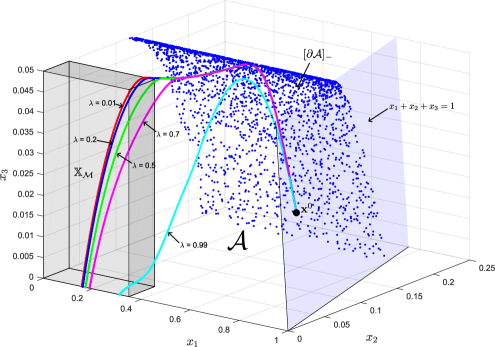
Figure 2: Closed-loop state trajectories of the constrained SEIR system, $\mathcal{S}$, produced by the MPC algorithm without terminal ingredients, Algorithm 3.1, with varying values for $\lambda$ (0.99 cyan, 0.7 magenta, 0.5 green, 0.2 dark blue, 0.01 red). The blue points indicate the boundary of the admissible set, $[\partial\mathcal{A}]_{-}:=\partial\mathcal{A}\cap\mathrm{int}(\mathbb{X})$; the grey box indicates the invariant box, $\mathbb{X}_{\mathcal{M}}$; and the blue plane indicates the set $\{\mathbf{x}\in\mathbb{R}^{3}:x_{1}+x_{2}+x_{3}=1\}$.

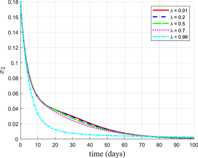
Figure 3: Closed-loop behaviour of the exposed compartment under the MPC feedback with varying $\lambda$ (first 100 days).

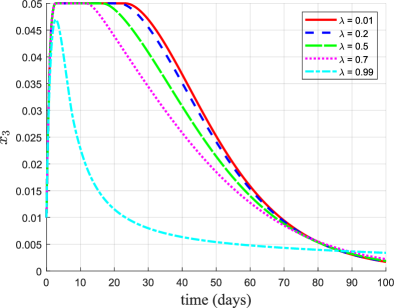
Figure 4: Closed-loop behaviour of the infectuous compartment under the MPC feedback with varying $\lambda$ (first 100 days).

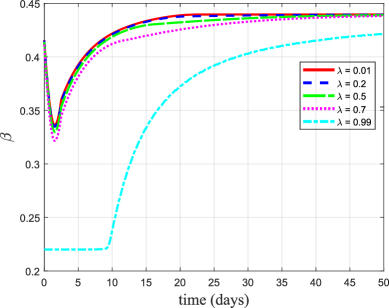
Figure 5: Closed-loop behaviour of $\beta$ with varying $\lambda$ (first 50 days).

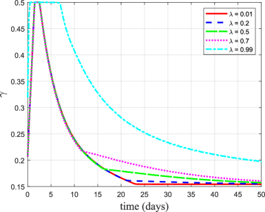
Figure 6: Closed-loop behaviour of $\gamma$ with varying $\lambda$ (first 50 days).

Table 1: The effect of $\lambda$ on the lifetime of the epidemic.

	Days until $\max\{x_{2}(t),x_{3}(t)\}<\mathrm{val}$
$\lambda$	$\mathrm{val}=10^{-5}$	$\mathrm{val}=10^{-6}$	$\mathrm{val}=10^{-7}$	$\mathrm{val}=10^{-8}$
0.01	186.5	225	263.75	302
0.2	188.75	228	267.5	306.5
0.5	196.75	239	281.25	323.75
0.7	212.25	260	307.5	355.25
0.99	612	801.25	988	1175

5 Conclusions an Perspectives

Drawing on results from [36], we rigorously showed that an SEIR epidemic can be eliminated via MPC without terminal ingredients provided that the state initiates from a suitable subset of the admissible set, one uses a suitable quadratic running cost, and the prediction horizon in the finite-horizon OCP is sufficiently long. Numerics suggest that this prediction horizon may be much shorter than the one required in MPC with terminal ingredients. Moreover, they showed that higher values of $\lambda$ in the cost functional, which penalise deviation from equilibrium points, result in fewer infected individuals but longer epidemics.

Future research could generalise the results to the case where the running cost, (9), is more elaborate, allowing certain state variables or intervention measures to carry more weight than others. We note that the use of a general quadratic cost (that is, one of the form $\ell(\mathbf{x},\mathbf{u})=\|\mathbf{x}\|_{Q}^{2}+\|\mathbf{u}-\mathbf{u}_{\mathrm{nom}}\|_{R}^{2}$ with $Q\succeq 0$ and $R\succ 0$) introduces cross terms, which make the proofs of some of the results more difficult.

Future research could also focus on generalisations of the paper’s results to more elaborate epidemic models. In particular, models where reinfection is possible (modelled, for example, as a flow from the removed compartment, $R$, to the susceptible compartment, $S$) are interesting for diseases like Covid-19. The main challenge introduced by such models is the fact that the susceptible compartment is not strictly decreasing over time, a fact we used extensively in deriving the results in this paper.

Appendix A Proof of Lemma 2

Proof 6

To ease notation throughout the proof, let $\mathbf{x}(t)=(x_{1}(t),x_{2}(t),x_{3}(t))^{\top}=\mathbf{x}(t;\mathbf{x}^{0},\mathbf{u}_{\mathrm{nom}})$ denote the “nominal” solution, and let $x_{i}^{\infty}=x_{i}^{\infty}(\mathbf{x}^{0},\mathbf{u}_{\mathrm{nom}})$, $i\in{1,2,3}$. Because $\mathbf{x}^{0}\in\mathbb{X}_{\mathcal{M}}$, by Lemma 1, we have that $\mathbf{x}(t)\in\mathbb{X}$ for all $t\geq 0$, with $x_{1}^{\infty}\in[0,1]$, and $x_{2}^{\infty}=x_{3}^{\infty}=0$. Therefore, noting that,

$$\int_{0}^{\infty}\beta_{\mathrm{nom}}x_{1}(t)x_{3}(t)\,\mathrm{d}t=-\int_{0}^{\infty}\dot{x}_{1}(t)\,\mathrm{d}t=x_{1}^{0}-x_{1}^{\infty}\in[0,1],$$

we see that,

$$\int_{0}^{\infty}x_{2}(t)\,\mathrm{d}t =\frac{1}{\eta}\left(\int_{0}^{\infty}\beta_{\mathrm{nom}}x_{1}(t)x_{3}(t)\,\mathrm{d}t-\int_{0}^{\infty}\dot{x}_{2}(t)\right)\,\mathrm{d}t$$

$$=\frac{1}{\eta}(x_{1}^{0}-x_{1}^{\infty}+x_{2}^{0})<\infty.$$

Similarly,

$$\int_{0}^{\infty}x_{3}(t)\,\mathrm{d}t =\frac{1}{\gamma_{\mathrm{nom}}}\left(\int_{0}^{\infty}\eta x_{2}(t)\,\mathrm{d}t-\int_{0}^{\infty}\dot{x}_{3}(t)\,\mathrm{d}t\right)$$

$$=\frac{1}{\gamma_{\mathrm{nom}}}\left(\eta\frac{1}{\eta}(x_{1}^{0}-x_{1}^{\infty}+x_{2}^{0})+x_{3}^{0}\right)<\infty.$$

Let $C:=\lambda\left(\frac{1}{\eta}(x_{1}^{0}-x_{1}^{\infty}+x_{2}^{0})+\frac{1}{\gamma_{\mathrm{nom}}}(x_{1}^{0}-x_{1}^{\infty}+x_{2}^{0}+x_{3}^{0})\right)<\infty$. Then, because $x_{2}(t),x_{3}(t)\in[0,1]$ for all $t\geq 0$, we see that,

$$J_{\infty}(\mathbf{x}^{0},\mathbf{u}_{\mathrm{nom}}) =\lambda\int_{0}^{\infty}\left(x_{2}^{2}(t)+x_{3}^{2}(t)\right)\,\mathrm{d}t$$

$$\leq\lambda\int_{0}^{\infty}\left(x_{2}(t)+x_{3}(t)\right)\ \mathrm{d}t$$

$$\leq C,\quad\forall\mathbf{x}^{0}\in\mathbb{X}_{\mathcal{M}}.$$

References

- [1] H. W. Hethcote, The mathematics of infectious diseases, SIAM Review 42 (4) (2000) 599–653.
- [2] F. Brauer, C. Castillo-Chavez, Z. Feng, Mathematical models in epidemiology, Springer, 2019.
- [3] J. L. Sanders, Quantitative guidelines for communicable disease control programs, Biometrics (1971) 883–893.
- [4] H. W. Hethcote, P. Waltman, Optimal vaccination schedules in a deterministic epidemic model, Mathematical Biosciences 18 (3-4) (1973) 365–381.
- [5] N. Gupta, R. Rink, Optimum control of epidemics, Mathematical Biosciences 18 (3-4) (1973) 383–396.
- [6] D. Kirschner, S. Lenhart, S. Serbin, Optimal control of the chemotherapy of HIV, Journal of Mathematical Biology 35 (7) (1997) 775–792.
- [7] H. Behncke, Optimal control of deterministic epidemics, Optimal Control Applications and Methods 21 (2000) 269–285.
- [8] E. Hansen, T. Day, Optimal control of epidemics with limited resources, Journal of Mathematical Biology 62 (2011) 423–451.
- [9] K. Kandhway, J. Kuri, How to run a campaign: Optimal control of SIS and SIR information epidemics, Applied Mathematics and Computation 231 (2014) 79–92.
- [10] F. B. Agusto, I. M. ELmojtaba, Optimal control and cost-effective analysis of malaria/visceral leishmaniasis co-infection, PLoS ONE 12 (2) (2017) e0171102.
- [11] L. Bolzoni, E. Bonacini, C. Soresina, M. Groppi, Time-optimal control strategies in SIR epidemic models, Mathematical Biosciences 292 (2017) 86–96.
- [12] P. Godara, S. Herminghaus, K. M. Heidemann, A control theory approach to optimal pandemic mitigation, PloS ONE 16 (2) (2021) e0247445.
- [13] V. S. Borkar, D. Manjunath, Revisiting SIR in the age of COVID-19: Explicit solutions and control problems, SIAM Journal on Control and Optimization 60 (2) (2022) S370–S395.
- [14] L. Chang, W. Gong, Z. Jin, G.-Q. Sun, Sparse optimal control of pattern formations for an SIR reaction-diffusion epidemic model, SIAM Journal on Applied Mathematics 82 (5) (2022) 1764–1790.
- [15] T. Britton, L. Leskelä, Optimal intervention strategies for minimizing total incidence during an epidemic, SIAM Journal on Applied Mathematics 83 (2) (2023) 354–373.
- [16] D. Goreac, J. Li, B. Xu, A stochastic jump model for epidemics with demography, and confinement and vaccination controls: Safety zones and algorithms, in: 2022 13th Asian Control Conference (ASCC), IEEE, 2022, pp. 197–202.
- [17] L. Freddi, D. Goreac, J. Li, B. Xu, SIR epidemics with state-dependent costs and ICU constraints: a Hamilton–Jacobi verification argument and dual LP algorithms, Applied Mathematics & Optimization 86 (2) (2022) 23.
- [18] F. Avram, L. Freddi, D. Goreac, Optimal control of a SIR epidemic with ICU constraints and target objectives, Applied Mathematics and Computation 418 (2022) 126816.
- [19] L. Grüne, J. Pannek, Nonlinear model predictive control: Theory and algorithms, 2nd Edition, Springer, 2017.
- [20] J. B. Rawlings, D. Q. Mayne, M. Diehl, Model predictive control: Theory, computation, and design, Nob Hill Publishing, 2017.
- [21] S. Grundel, S. Heyder, T. Hotz, T. K. Ritschel, P. Sauerteig, K. Worthmann, How much testing and social distancing is required to control COVID-19? Some insight based on an age-differentiated compartmental model, SIAM Journal on Control and Optimization 60 (2) (2022) S145–S169.
- [22] S. Grundel, S. Heyder, T. Hotz, T. K. S. Ritschel, P. Sauerteig, K. Worthmann, How to Coordinate Vaccination and Social Distancing to Mitigate SARS-CoV-2 Outbreaks, SIAM Journal on Applied Dynamical Systems 20 (2) (2021) 1135–1157.
- [23] J. Köhler, L. Schwenkel, A. Koch, J. Berberich, P. Pauli, F. Allgöwer, Robust and optimal predictive control of the COVID-19 outbreak, Annu. Rev. Control (2020).
- [24] F. Sélley, Á. Besenyei, I. Z. Kiss, P. L. Simon, Dynamic control of modern, network-based epidemic models, SIAM Journal on Applied Dynamical Systems 14 (1) (2015) 168–187.
- [25] M. M. Morato, S. B. Bastos, D. O. Cajueiro, J. E. Normey-Rico, An optimal predictive control strategy for COVID-19 (SARS-CoV-2) social distancing policies in Brazil, Annual reviews in control 50 (2020) 417–431.
- [26] F. Parino, L. Zino, G. C. Calafiore, A. Rizzo, A model predictive control approach to optimally devise a two-dose vaccination rollout: A case study on COVID-19 in Italy, International Journal of Robust and Nonlinear Control (2021).
- [27] J. Köhler, C. Enyioha, F. Allgöwer, Dynamic resource allocation to control epidemic outbreaks a model predictive control approach, in: 2018 Annual American Control Conference (ACC), IEEE, 2018, pp. 1546–1551.
- [28] N. J. Watkins, C. Nowzari, G. J. Pappas, Robust economic model predictive control of continuous-time epidemic processes, IEEE Transactions on Automatic Control 65 (3) (2020) 1116–1131.
- [29] P. Sauerteig, W. Esterhuizen, M. Wilson, T. K. Ritschel, K. Worthmann, S. Streif, Model predictive control tailored to epidemic models, in: European Control Conference (ECC), IEEE, 2022, pp. 743–748.
- [30] J. A. De Dona, J. Lévine, On barriers in state and input constrained nonlinear systems, SIAM Journal on Control and Optimization 51 (4) (2013) 3208–3234.
- [31] W. Esterhuizen, T. Aschenbruck, S. Streif, On maximal robust positively invariant sets in constrained nonlinear systems, Automatica 119 (2020) 109044.
- [32] W. Esterhuizen, J. Lévine, S. Streif, Epidemic management with admissible and robust invariant sets, PLoS ONE 16 (9) (2021) e0257598.
- [33] D. Q. Mayne, Model predictive control: Recent developments and future promise, Automatica 50 (12) (2014) 2967–2986.
- [34] E. D. Sontag, Mathematical control theory: Deterministic finite dimensional systems, Springer Science & Business Media, 2013.
- [35] J.-P. Aubin, A. M. Bayen, P. Saint-Pierre, Viability theory: New directions, Springer Science & Business Media, 2011.
- [36] W. Esterhuizen, K. Worthmann, S. Streif, Recursive feasibility of continuous-time model predictive control without stabilising constraints, IEEE Control Systems Letters 5 (1) (2020) 265–270.
- [37] J. Berberich, J. Köhler, F. Allgöwer, M. A. Müller, Indefinite linear quadratic optimal control: Strict dissipativity and turnpike properties, IEEE Control Systems Letters 2 (3) (2018) 399–404.
- [38] J. Köhler, M. N. Zeilinger, L. Grüne, Stability and performance analysis of NMPC: Detectable stage costs and general terminal costs, IEEE Transactions on Automatic Control 68 (10) (2023).
- [39] L. Cesari, Optimization—theory and applications: Problems with ordinary differential equations, Springer Science & Business Media, 2012.
- [40] J. Macki, A. Strauss, Introduction to optimal control theory, Springer Science & Business Media, 2012.
- [41] J.-M. Coron, L. Gruüne, K. Worthmann, Model predictive control, cost controllability, and homogeneity, SIAM Journal on Control and Optimization 58 (5) (2020) 2979–2996.
- [42] L. Grüne, J. Pannek, M. Seehafer, K. Worthmann, Analysis of unconstrained nonlinear MPC schemes with time varying control horizon, SIAM Journal on Control and Optimization 48 (8) (2010) 4938–4962.
- [43] H. K. Khalil, Nonlinear systems, 3rd Edition, Prentice Haill, 2002.
- [44] M. Gerdts, Optimal control of ODEs and DAEs, De Gruyter, 2012.