Gated Chemical Units

Abstract

We introduce Gated Chemical Units (GCUs), a new type of gated recurrent cells which provide fresh insights into the commonly-used gated recurrent units, and bridge their gap to biologically-plausible neural models. We systematically derive GCUs from Electrical Equivalent Circuits (EECs), a widely adopted ordinary-differential-equations model in neuroscience for biological neurons with both electrical and chemical synapses. We focus on saturated EECs, as they are more stable, and chemical synapses, as they are more expressive. To define GCUs, we introduce a new kind of gate, we call a time gate (TG), in the associated difference-equations model of the EECs. The TG learns for each neuron the optimal time step to be used in a simple Euler integration scheme, and leads to a very efficient gated unit. By observing that the TG corresponds to the forget gate (FG) in traditional gated recurrent units, we provide a new formulation of these units as neural ODEs. We also show that in GCUs, the FG is in fact its liquid time constant. Finally, we demonstrate that GCUs not only explain the elusive nature of gates in traditional recurrent units, but also represent a very competitive alternative to these units.

1 Introduction

In this paper we introduce Gated Chemical Units (GCUs), a new type of gated recurrent units, which we formally derive from Electrical Equivalent Circuits (EECs), the main neuron model of neuroscience (Kandel et al., 2000; Wicks et al., 1996). This way, we connect the true biological nature of neurons to gated recurrent neural networks, for the first time.

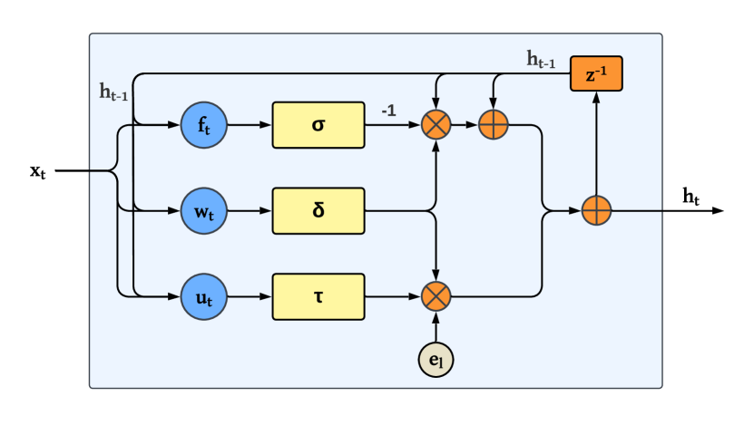
Figure 1: Architecture of a Gated Chemical Unit (GCU), with a sigmoidal forget gate $\sigma(f_{t})$, with a hyperbolic-tangent update $\tau(u_{t})$, and with a sigmoidal (a)symmetric time gate $\delta(w_{t})$.

Achieving a tight balance between biological relevance, efficiency, and interpretability, is a challenging research area in the development of neural-network architectures. Gated Recurrent Neural Networks (RNNs), which are computational models with a loose connection to biological processes, are widely used in time-series tasks in a variety of fields including communication, finance, and control engineering, thanks to their design of appropriate gating mechanisms. To apply them to safety-critical problems, there is a strong need for a formal underpinning, interpretability, and robustness.

Gated RNNs have various forms, which often came about from empirical evaluations that lack fundamental principles of why they work well. Long Short-Term Memory (LSTMs) (Hochreiter & Schmidhuber, 1997) were the first type of gated RNNs, designed to model long-term dependencies in sequential data, by using three gating mechanisms. Several attempts have been made to understand and further simplify their structure, with systematic evaluations of 8 variants of them in Greff et al. (2016). Gated Recurrent Units (GRUs) (Cho et al., 2014) employ a simplified structure with fewer parameters, reduced to two gates, thus providing computational efficiency compared to the more complex LSTMs. Similarly to LSTMs, new variants of GRUs have been tested to understand the significance of their components (Józefowicz et al., 2015). In particular, Minimal Gated Units (MGUs) (Zhou et al., 2016), further decrease the number of gates to one, but interestingly, they have a comparable performance to LSTMs and GRUs.

To capture the electrical behavior of biological neurons in a formal mathematical fashion, neuro-scientists use ordinary-differential-equations models (ODEs), called EECs (Kandel et al., 2000; Wicks et al., 1996). Chemical synapses are also called Liquid Time Constant Neural Networks (LTCs) in Lechner et al. (2019); Hasani et al. (2020); Lechner et al. (2020), due to the state-and-input dependent nature of their time constant. These neural-ODE models are biologically plausible by construction, but solving them is most often very challenging. This is due to the stiff, nonlinear nature of the ODEs, which is characterized by solutions with widely varying timescales. Consequently, adaptive numerical-integration methods, balancing between accuracy and efficiency, are often computationally expensive.

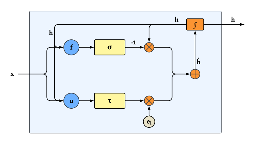
Figure 2: Architecture of the saturated Electrical-Equivalent Circuits (EECs) for biological neurons with chemical synapses.

The stiffness of EECs can be slightly reduced as shown in Farsang et al. (2023), by saturating the EEC (extended) conductances to range between -1 and 1, a normalization approach inspired by the various regulation mechanisms present in biological neurons. However, solving saturated EECs still remained very challenging, and the choice of the solver thus significantly impacted the learning efficiency.

In this paper, we show that a surprisingly simple but unorthodox approach, can be used to tame the stiffness of saturated chemical-synapse EECs, within a simple Euler integration scheme. The main idea is to use a gate, which we call a Time Gate (TG), in order to learn the optimal time step, for every neuron and every integration step. We call the resulting cells, Gated Chemical Units (GCUs). Our approach not only leads to a very efficient recurrent biological unit, but also elucidates the elusive role of the Forget Gate (FG) in traditional gated recurrent units. Moreover, restating the FG as a TG in these units, allows us to provide a fresh and new look at them, in form of Neural ODEs. In the context of GCUs, we also show that the true nature of the FG is their liquid time constant. Finally, by employing the standard benchmarks developed for gated RNNs, we demonstrate that GCUs provide a very competitive alternative, that has a robust, interpretable, and formal biological underpinning.

In summary, the main results of our paper are as follows:

• We introduce Gated Chemical Units (GCUs), which establish the formal connection between biological-neuron models and gated RNNs, for the first time.

• We systematically derive GCUs from chemical-synapse EECs, an ODEs model used in neuro-science, by considering saturation and adding a new time gate.

• We provide a novel view of traditional gated RNNs as various instances of neural ODEs, by identifying their forget gate with our newly-introduced time gate.

• We show that in the context of GCUs, the forget gate actually corresponds to a separate and distinct gate, capturing the liquid time constant of the GCUs.

• Our experimental results on a wide range of benchmarks, demonstrate that GCUs achieve very competitive results, compared to traditional gated RNNs.

The rest of this paper is organized as follows. In Section 2 we review saturated, chemical-synapse EECs. In Section 3 we discuss EECs integration and introduce the time gate. In Section 4 we give a fresh view of gated recurrent units as Neural ODEs. In Section 5 we provide our experimental results. Finally, in Section 6 we discuss our conclusions.

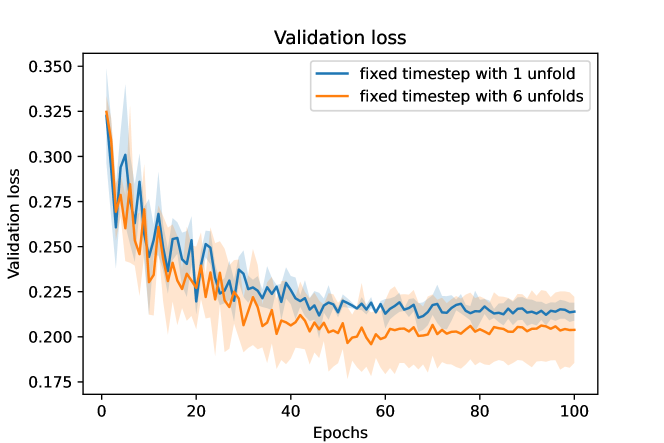
Figure 3: Validation loss of saturated, chemical EECs for the Lane-Keeping Task with a fixed time step, using either a single unfolding step (blue) or 6 unfoldings, by dividing the time step by 6 (orange).

2 Background on Saturated EECs

EECs capture the relation between the membrane potentials (states) of pre- and post-synaptic neurons, respectively, for either electrical or chemical synapses (Kandel et al., 2000; Wicks et al., 1996). Previous work showed that a saturated variant of chemical-synapse EECs with $m$ states and $n$ inputs, is described by the ODEs below (Farsang et al., 2023):

$$\begin{array}[]{c}\dot{h}_{i}=-\sigma(f_{i})\,h_{i}+\tau(u_{i})\,e_{li}\\[8.53581pt] f_{i}=\sum_{j=1}^{m+n}g_{ji}\sigma(a_{ji}y_{j}+b_{ji})+g_{li}\\[5.69054pt] u_{i}=\sum_{j=1}^{m+n}k_{ji}\sigma(a_{ji}y_{j}+b_{ji})+g_{li}\end{array}$$ (1)

The architecture of the EECs in Equations (1) is given in Figure 2. They state that the rate of change of the membrane potential $h_{i}$ of neuron $i$, is the sum of its negative forget current $-\sigma(f_{i})\,h_{i}$ and its update current $\tau(u_{i})\,e_{li}$. Hence, the conductance $\sigma(f_{i})$, is the liquid time constant of $h_{i}$. In the rest of the paper, we call $\sigma(f_{i})$, the Forget Gate (FG) of the EECs, and $\tau(u_{i})$, the update part of the EECs.

The sigmoid $\sigma$ enclosing the forget conductance $f_{i}$ of neuron $i$, saturates it to range within $[0,1]$. This depends on the state $h_{j}$ of presynaptic neurons $j$, and inputs $x_{j}$, and thus on $y\,{=}\,[h,x]$. Here, $g_{ji}$ is the maximum conductance of neuron $i$ synaptic channels, and $a_{ji},b_{ji}$ are parameters controlling the sigmoidal probability of these channels to be open. Finally, $g_{li}$ is the membrane’s leaking conductance.

The hyperbolic tangent $\tau$ enclosing the signed state-input dependent update conductance $u_{i}$, saturates it to range within $[-1,1]$. Here, $k_{ji}\,{=}\,g_{ji}{/}e_{ji}$ takes the sign of $e_{ji}$, which is the channels’ reversal potential, that is, the membrane potential at which there is no net flow through the channels.

Solving saturated, chemical-synapse EECs with popular ODE-integration techniques, is still computationally expensive. A hybrid forward-backward Euler method (Lechner et al., 2020) for example, takes multiple unfolding rounds for a given input, to achieve a good approximation of the solution. In Figure 3 we show the validation loss of saturated EECs, for the Lane-Keeping Task (Lechner et al., 2022), where the state of the neurons is computed with a fixed integration step $\delta_{t}$. Diving this into 6 equidistant time steps $\delta_{t}{/}6$ within one update step, results in a considerably better model, but at a higher cost of 622s versus 241s per epoch. This results in a $2.6\times$ longer computation time.

3 Integration Step as a Time Gate

Given the saturated, chemical-synapse EECs in Equation 1, and assuming the use of a simple, Euler integration scheme with a time-varying step $\delta_{i,t}$ for each neuron, we can rewrite the EECs as a set of ordinary difference equations as below:

$$\begin{array}[]{c}h_{i,t}=(1-\sigma(f_{i,t})\,\delta_{i,t})\,h_{i,t-1}+\tau(u_{i,t})\,\delta_{i,t}\,e_{li}\\[8.53581pt] f_{i,t}=\sum_{j=1}^{m+n}g_{ji}\sigma(a_{ji}y_{j,t}+b_{ji})+g_{li}\\[5.69054pt] u_{i,t}=\sum_{j=1}^{m+n}k_{ji}\sigma(a_{ji}y_{j,t}+b_{ji})+g_{li}\end{array}$$ (2)

We regard Equations (2), as the model of a recurrent controller (including state estimation), and the inputs $x$ as observations of its environment. We thus define $y_{t}\,{=}\,[h_{t-1},x_{t}]$ in the forget and update conductances. This way, $y_{t}$ contains the current, instead of the previous observation, respectively.

The first question this paper now asks, and solves in a surprisingly simple way, is how to compute $\delta_{i,t}$ such that we obtain a very efficient and fast-converging integration scheme?

One simple technique, known to physicists for a long time, and discussed in Shampine & Witt (1995), is to keep the change of $dh_{i,t}$ in $\dot{h}_{i,t}\,{=}\,dh_{i,t}/dt$, fixed to a constant $c_{i}$. This technique results in a first approximation of $\delta_{i,t}$ as $w_{i,t}\,{=}\,c_{i}/(|\dot{h}_{i,t}|\,{+}\,\epsilon_{i})$, where a small $\epsilon_{i}$ is used to avoid division by zero. Let us further scale $w_{i,t}$ to range between $[0,1]$, symmetrically with regards to $\dot{h}$, with either a hyperbolic tangent or a difference of sigmoids, respectively. Finally, if the time interval $\Delta_{t}$ between two successive inputs in the time series $x$ is available, and it is different from unit $1$, we use this to multiply $w_{i,t}$ as in Equations (4-5). They are the first approximations of our Time Gate (TG):

$$w_{i,t}\,{=}\,c_{i}/(|\dot{h}_{i,t}|\,{+}\,\epsilon_{i})\vspace*{-1mm}$$ (3)

$$\delta_{i,t}=\tau(w_{i,t}\,\Delta_{t})\vspace*{-1mm}$$ (4)

$$\delta_{i,t}=\sigma(w_{i,t}\Delta_{t}+k_{i})-\sigma(-w_{i,t}\Delta_{t}+k_{i})$$ (5)

In general, it is hard to find the adequate values for $c_{i}$, $\epsilon_{i}$, and $k_{i}$. We solve this problem, by simply learning them. This is memory efficient, as it only requires $3m$ parameters.

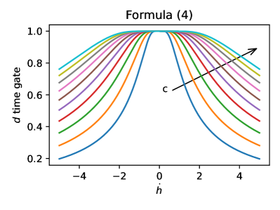
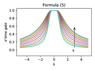
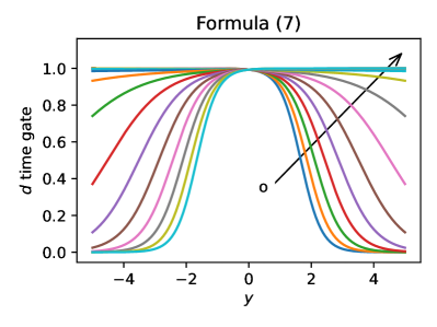
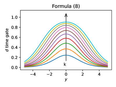
Figure 4: The shape of the various time-gates proposed for GCUs, using Formulas (3-5) on the top, and Formulas (6-8) on the bottom.

We found however, that a TG learned from scratch, and scaled with regard to $y$, either asymmetrically, with one sigmoid, or symmetrically, with a difference of sigmoids, leads to considerably better results in terms of accuracy and convergence speed. Define the first approximation of the time step as $w_{i,t}\,{=}\,\sum_{j=1}^{m+n}o_{ji}y_{j,t}\,{+}\,p_{j}$. Then the asymmetric and symmetric TGs learned from scratch, respectively, are given by the Equations (7-8). While these solutions are more costly in terms of parameters, as one has to learn the matrix $o$ and the vectors $p,k$, the cost is clearly worth it.

$$\begin{array}[]{c}w_{i,t}=\sum_{j=1}^{m+n}o_{ji}y_{j,t}+p_{j}\end{array}$$ (6)

$$\delta_{i,t}=\sigma(w_{{i,t}}\Delta_{t})\\ \vspace*{-1mm}$$ (7)

$$\delta_{i,t}=\sigma(w_{i,t}\Delta_{t}+k_{i})-\sigma(w_{i,t}\Delta_{t}-k_{i})$$ (8)

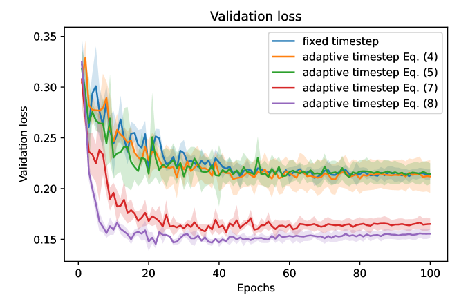
Figure 5: Validation loss of the RNN for the Lane-Keeping Task with a fixed time step, and the four time steps of Equations (3-8). The results for the TGs in Equations (4-5) are rather disappointing. However, the results for the TGs in Equations (7-8) are very encouraging, both in terms of accuracy and convergence speed.

In Figure 5, we compare the validation loss of the RNN defined by Equations (2), for the Lane-Keeping Task, where we compute the time step $\delta_{i,t}$ in five different ways. In the first, as a baseline, we use a constant time-step of size $1$. In the next two, we use Equations (4-5), where we learn the parameters $c$, $\epsilon$, and $k$. Finally, in the last two, we use Equations (7-8), where we learn the parameters $o$, $p$, and $k$.

The results for the TGs defined by Equations (4-5) are rather disappointing, as they do not visibly improve baseline’s accuracy and convergence speed. While each neuron adapts its time step in accordance with its current derivative $\dot{h}_{i,t}$, it still keeps its change of state $dh_{i,t}$ fixed to a learned constant value $c_{i}$. One can generalize this TG by replacing constant $c_{i}$ with a function $c_{i,t}\,{=}\,c_{i}(y_{i,t})$, which similarly to $\dot{h}_{i,t}$ depends on $y_{i,t}$, resulting in a nonlinear time step $w_{i,t}=c_{i,t}\,/\,(|\dot{h}_{i,t}|+\epsilon_{i})$. This time step however, can be learned directly, as the scaled (a)symmetric TGs of Equations (7-8). Using these TGs leads to a considerably faster convergence, with a much smaller loss. In particular, the symmetric TG achieves the best results, by essentially converging in less than 10 epochs, to a loss of about 0.15. The baseline instead, converges in about 60 epochs, at a loss of 0.22.

From now on, we will refer to the RNN defined by the Equations (2,7-8), as a Gated Chemical Unit (GCU) employing either an (7) asymmetric, or a (8) symmetric TG, respectively. The architecture of the GCU is provided in Figure 1.

4 Gated Recurrent Units as Neural ODEs

Starting from the Neural-ODEs model of saturated biological neurons with chemical synapses (the saturated EECs), we have shown that by first discretizing the ODEs in the form of ordinary difference equations, and then by learning their optimal-integration time step with a TG, leads to a very accurate and efficient gated RNN, which we called a GCU.

For a linear ODE with state $h$, it is common practice to call the constant, linearly multiplying the state, the time constant of the ODE. This constant determines the rate at which the ODE forgets its initial state. In GCUs, the time constant becomes liquid, as it is a function of the state and the input.

In the following, we call this liquid time constant, the Forget Gate (FG) of the GCU, as it is responsible for forgetting in the associated EEC, and thus in the formally derived GCU.

Once GCUs are formally derived, it is naturally to ask how do they relate to the popular gated RNNs? As mentioned in Zhou et al. (2016), the most important gate of these RNNs is their FG. This however, appears in the same parts of the RNNs, and in the same form, as our asymmetric, sigmoidal TG. This is very intriguing and requires further scrutiny.

The second question we thus ask in this paper, and answer in a positive fashion, is whether the commonly-used gated RNNs are in fact discretized forms of Neural ODEs, too?

In order to answer this question, we first identify a particular gate in the GRU, MGU, and LSTM architectures, with the asymmetric TG of GCUs. We then investigate what would be in this case their associated Neural ODEs. We first analyse GRUs, then continue with MGUs, as they can be seen as a simplification of GRUs, and conclude with LSTMs, as they are the most sophisticated. Finally, we compare these simpler Neural-ODE versions to biological EECs.

Gated recurrent units (GRUs).

The general form of a GRU is defined as below in Cho et al. (2014):

$$\begin{array}[]{c}h_{i,t}=(1-\sigma(f_{i,t}))\,h_{i,t-1}+\sigma(f_{i,t})\,\tau(u_{i,t})\\[8.53581pt] f_{i,t}=\sum_{j=1}^{m+n}a^{f}_{ji}\,y_{j,t}+b^{f}_{j}\\[5.69054pt] r_{i,t}=\sum_{j=1}^{m+n}a^{r}_{ji}\,y_{j,t}+b^{r}_{j}\\[5.69054pt] u_{i,t}=\sum_{j=1}^{m+n}a^{u}_{ji}\,y^{\prime}_{j,t}+b^{u}_{j}\end{array}$$ (9)

Here the vector $y_{t}$ occurring in functions $f_{i,t}$ and $r_{i,t}$, is defined as before, as $y_{t}\,{=}\,[h_{t-1},x_{t}]$. However, the vector $y^{\prime}_{t}$ occurring in $u_{i,t}$ is defined as $y^{\prime}_{t}\,{=}\,[\sigma(r_{t})\odot{}h_{t-1},x_{t}]$.

In other words, the previous state $h_{t-1}$ used in the update part $\tau(u_{i,t})$ of the GRU, is pointwise scaled with a nonlinear state-and-input dependent function $\sigma(r_{i,t})$, whose parameters are to be learned. This function is called in GRUs a Reset Gate (RG). Moreover, the state-and-input dependent function $\sigma(f_{i,t})$ is called in GRUs an Update Gate (UG).

The RG determines how the previous state $h_{t-1}$ has to be used in the update $\tau(u_{i,t})$. The UG $\sigma(f_{i,t})$ controls the amount $(1-\sigma(f_{i,t}))$ of the previous state $h_{i,t-1}$, to be remembered in the next state. However, this UG also controls the amount of the update $\tau(u_{i,t})$ to be considered in the next state, by using it to multiply the update.

This affine combination of previous state and update with respect to GRU’s UG, remains quite elusive, until one identifies the GRU’s UG with the GCU’s TG. Indeed, if no information about the time intervals within the input $x$ is available, and thus if $\Delta_{t}$ is 1, the GRU’s UG $\sigma(f_{i,t})$, is identical to the GCU’s TG. Moreover, as a time step in the ordinary difference equation associated to an ODE, the affine occurrence of the GRU’s UG makes perfectly sense.

Given the above discussion, GRUs can also be understood as the ordinary difference equations associated to the Neural ODEs below, where the optimal time steps are learned:

$$\begin{array}[]{c}\dot{h}_{i}=-h_{i}+\tau(u_{i})\\[5.69054pt] r_{i}=\sum_{j=1}^{m+n}a^{r}_{ji}\,y_{j}+b^{r}_{j}\\[5.69054pt] u_{i}=\sum_{j=1}^{m+n}a^{u}_{ji}\,y^{\prime}_{j}+b^{u}_{j}\end{array}$$ (10)

Here the vector $y\,{=}\,[h,x]$ is defined as before, and vector $y^{\prime}\,{=}\,[\sigma(r)\odot{}h,x]$. The RG occurring in $y^{\prime}$ determines how to use state $h$ in the update part $\tau(u_{i})$ of the ODE.

The time constant of the GRU’s neural ODEs however, is simply taken to be 1. In other words, the GRU discards the fixed information $h$ from the next state. As a consequence, GRUs are less expressive compared to GCUs, where the time constant is liquid, and thus, the amount of previous state discarded depends on both the input $x$ and the state $h$.

Minimal gated units (MGUs).

The general form of an MGU is defined as below in (Zhou et al., 2016):

$$\begin{array}[]{c}h_{i,t}=(1-\sigma(f_{i,t}))\,h_{i,t-1}+\sigma(f_{i,t})\,\tau(u_{i,t})\\[8.53581pt] f_{i,t}=\sum_{j=1}^{m+n}a^{f}_{ji}\,y_{j,t}+b^{f}_{j}\\[5.69054pt] u_{i,t}=\sum_{j=1}^{m+n}a^{u}_{ji}\,y^{\prime}_{j,t}+b^{u}_{j}\end{array}$$ (11)

Here, vector $y_{t}$ is defined as before as $y_{t}\,{=}\,[h_{t-1},x_{t}]$, and $y^{\prime}_{t}$ is defined as $y^{\prime}_{t}\,{=}\,[\sigma(f_{t})\odot{}h_{t-1},x_{t}]$, that is, the previous state $h_{t-1}$ is pointwise multiplied with the function $\sigma(f_{t})$.

As one can see from Equations (11), the MGU definition simplifies the GRU definition, by insisting that the RG $\sigma(r_{t})$ and the UG $\sigma(f_{t})$ of the GRUs should be identified as one and the same gate $\sigma(f_{t})$ in MGUs. This gate is is called a Forget Gate (FG) in MGUs, as it controls the amount $(1-\sigma(f_{i,t}))$ of the previous state $h_{i,t-1}$, to be remembered in the next state. However, as already mentioned, this FG also controls the amount of update $\tau(u_{i,t})$ to be considered in the next state, by multiplying the update. As a consequence we identify the FG of MGUs, with the TG of GCUs.

Given the above considerations, the MGU can be understood as the ordinary difference equations associated to the Neural ODEs below, where the optimal time step is learned:

$$\begin{array}[]{c}\dot{h}_{i}=-h_{i}+\tau(u_{i})\\[5.69054pt] u_{i}=\sum_{j=1}^{m+n}k_{ji}y^{\prime}_{j}+l_{j}\end{array}$$ (12)

Here $y^{\prime}\,{=}\,[dt\odot{}h,x]$. This is a somewhat tricky ODE, where the term $dt$ in $dt\odot{}h$ can be understood as a quite refined hint to the ODE integrator, to scale the previous state $h$ within the update part $\tau(u_{i})$ of the ODEs, with the same TG as the one used for the time step. Since this identification works well, $dt$ might indeed be the proper gate for multiplying $h$.

As for the GRUs, the time constant of the Neural ODEs associated to the MGUs, is 1. As a consequence, the control of forgetfulness in MGUs, is considerably less expressive compared to GCUs, where the time constant is liquid.

Long Short-Term Memory (LSTM).

These RNNs are the most complex of the examined gated RNNs. They are defined as follows (Hochreiter & Schmidhuber, 1997):

$$\begin{array}[]{c}c_{i,t}=\sigma(f_{i,t})\,c_{i,t-1}+\sigma(i_{i,t})\,\tau(u_{i,t})\\[2.84526pt] h_{i,t}=\sigma(o_{i,t})\,\tau(c_{i,t})\\[8.53581pt] f_{i,t}=\sum_{j=1}^{m+n}a^{f}_{ji}\,y_{j,t}+b^{f}_{j}\\[5.69054pt] i_{i,t}=\sum_{j=1}^{m+n}a^{i}_{ji}\,y_{j,t}+b^{i}_{j}\\[5.69054pt] o_{i,t}=\sum_{j=1}^{m+n}a^{o}_{ji}\,y_{j,t}+b^{o}_{j}\\[5.69054pt] u_{i,t}=\sum_{j=1}^{m+n}a^{u}_{ji}\,y_{j,t}+b^{u}_{j}\end{array}$$ (13)

An LSTM distinguishes between a recurrent cell state $c_{i,t}$ and an algebraic hidden state $h_{i,t}$. These states are related to each other, by defining the hidden state $h_{i,t}$ as the pointwise product of the Output Gate (OG) $\sigma(o_{i,t})$ with the scaled cell state $\tau(c_{i,t})$. The two other gates are called the Forget Gate (FG) $\sigma(f_{i,t})$ and the Input Gate (IG) $\sigma(i_{i,t})$. They determine the next cell’s state, by forgetting part of the previous cell’s state and adapting the update information, respectively. Finally the state-and-input vector equals $y_{t}\,{=}\,[h_{t-1},x_{t}]$.

In order to derive the Neural ODEs associated to an LSTM one has the following complication: the next cell state $c_{i,t}$ of the LSTM is not an affine combination of the previous cell state $c_{i,t-1}$ and the update $\tau(u_{i,t})$, with respect to a given gate. Instead, the previous cell state $c_{i,t-1}$ is multiplied by the FG, and the update $\tau(u_{i,t})$ is multiplied by the IG. One can however obtain the desired affine combination, in two steps. First, by using the identity $\sigma(-i_{i,t})=1-\sigma(i_{i,t})$. Second, by relating the gates with $\sigma(f_{i,t})=\sigma(-i_{i,t})$. Using this approach, one obtains the following ODEs:

$$\begin{array}[]{c}\dot{c}_{i}=-c_{i}+\tau(u_{i})\\[2.84526pt] h_{i}=\sigma(o_{i})\,\tau(c_{i})\\[5.69054pt] o_{i,}=\sum_{j=1}^{m+n}a^{o}_{ji}\,y_{j}+b^{o}_{j}\\[5.69054pt] u_{i}=\sum_{j=1}^{m+n}a^{u}_{ji}\,y_{j}+b^{u}_{j}\end{array}$$ (14)

where the vector $y\,{=}\,[h,x]$ and $\sigma(f)+\sigma(i)=1$. If the latter equality holds, one essentially obtains the Neural ODE of the GRUs. If it does not, one can still derive a Neural ODE, by using the identity $\sigma(f_{i})=1-\sigma(-f_{i})$ and by replacing the differential equation above in the following way:

$$\vspace*{-3mm}\begin{array}[]{c}\dot{c}_{i}=-c_{i}+\frac{\sigma(i_{i})}{dt}\,\tau(u_{i})\\[2.84526pt] i_{i}=\sum_{j=1}^{m+n}a^{i}_{ji}\,y_{j}+b^{i}_{j}\\ \end{array}$$ (15)

The differential Equations (15), together with the three algebraic equations of the ODEs defined in (14), give the most general form of the Neural ODEs associated to LSTMs. As it was the case for MGUs, the $dt$ term occurring in above equations, can be understood as hint to the integrator, to divide the IG $\sigma(i_{i})$ of the update, with the TG $\sigma(-f_{i})$. This makes perfectly sense, as one divides in principle two TGs.

Table 1: Accuracy results for the irregularly sampled person activity classification dataset. To achieve a somewhat similar number of trainable parameters, we employed 64 cells for GCUs and 100 cells in the other models. We repeated the experiments 5 times.

Model	Accuracy	No. of param.
LSTM	$82.90\%\pm 0.31\%$	40k
GRU	$82.76\%\pm 0.41\%$	30k
MGU	$83.35\%\pm 0.30\%$	20k
GCU-STG	$\mathbf{84.99\%\pm 0.59\%}$	20k
GCU-ATG	$84.96\%\pm 0.40\%$	20k

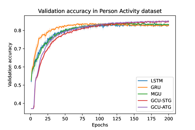
Figure 6: Validation accuracy for the irregularly sampled person activity dataset. GCUs converge a bit slower, yet they surpass the validation accuracy of the other models after 100 epochs.

Relationship among GCUs, GRUs, MGUs, and LSTMs.

As discussed in the previous paragraph, the general differential equation of LSTMs given in (15), simplifies to the one of GRUs and MGUs, if the LSTM’s IG and FG sum up to 1.

Moreover, in these gated RNNs, the time constant of the associated Neural ODEs is 1. This is less expressive compared to the GCUs, as GCUs have instead a liquid time constant, that is, a function which depends on both the input and the state. We argued that this function is a proper FG, as it determines the rate at which the previous state of the ODEs is forgotten. The FG of the other RNNs is thus trivial.

LSTMs multiply the scaled cell state with the output gate in the vector $y\,{=}\,[\sigma(o)\odot\tau(c),x]$ when computing both the IG $\sigma(i)$ and the update $\tau(u)$. In GRUs, the update $\tau(u)$ also scales the state with the RG, that is, $y\,{=}\,[\sigma(r)\odot{}h,x]$, but the UG of the GRU uses the simpler version $y\,{=}\,[h,x]$. Finally, in MGUs, the FG gate uses $y\,{=}\,[h,x]$, but the update $\tau(u)$ uses $y\,{=}\,[dt\odot{}h,x]$. GCUs have in this respect the simplest update $\tau(u)\,e_{l}$, where $u$ is computed using $y\,{=}\,[h,x]$.

In conclusion, GCUs, LSTMs, GRUs, and MGUs, all employ a sigmoidal TG, to compute the optimal time step, when integrating their associated Neural ODEs. GCUs also propose a symmetric form of TG, as a difference of sigmoids. GCUs are the only ones to possess a proper FG, in form of their liquid time constant. The FG of the other is trivial, and equal to 1. LSTMs, GRUs, and MGUs however, compensate for the lack of a proper FG, by using a gate to scale the state used in the update part of the Neural ODEs.

Table 2: Accuracy results for the IMDB sentiment classification problem. We used 64 cells in the GCUs and 100 cells in the other models. Note that, the total number of parameters is influenced by input and output, too. All the results are averaged over 3 runs.

Model	Accuracy	No. of param.
LSTM	$86.56\%\pm 0.49\%$	70k
GRU	$86.32\%\pm 0.51\%$	50k
MGU	$85.18\%\pm 0.85\%$	35k
GCU-STG	$85.73\%\pm 0.41\%$	40k
GCU-ATG	$\mathbf{87.00\%\pm 0.53\%}$	40k

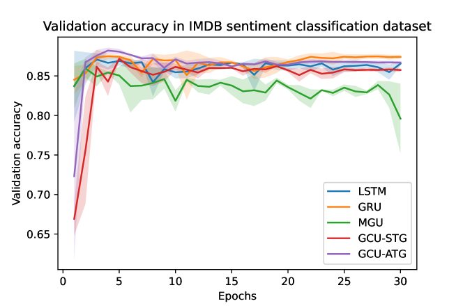
Figure 7: Validation accuracy for the IMDB sentiment classification problem. The GCU-ATG achieves the highest accuracy after only 5 epochs, even though this decreases a bit over time.

Synaptic versus neural activation in GCUs.

In the EECs describing the behavior of biological neurons with chemical synapses, each synapse has its own sigmoidal activation, which corresponds to the probability of its synaptic channels to be open. This is reflected in the parameters $a_{ji}$ and $b_{ji}$ of the sigmoids. Consequently, EECs have more parameters. If one assumes however, that all the outgoing synapses of a neuron behave the same way, one can simplify the EECs by computing the activation only once per neuron, as it is customary in artificial neural networks. This leads to EECs:

$$\begin{array}[]{c}\dot{h}_{i}=-\sigma(f_{i})\,h_{i}+\tau(u_{i})\,e_{li}\\[8.53581pt] f_{i}=\sum_{j=1}^{m+n}g_{ji}\sigma(a_{j}y_{j}+b_{j})+g_{li}\\[5.69054pt] u_{i}=\sum_{j=1}^{m+n}k_{ji}\sigma(a_{j}y_{j}+b_{j})+g_{li}\end{array}$$ (16)

The additional flexibility of the synaptic activation, which is motivated by the behavior of biological neurons, not only improves the accuracy of the resulting GCUs (even when one considers the same number of parameters in the synaptic and neural-activation models, respectively), but also increases the interpretability of the learned GCUs. We therefore use GCUs with synaptic activation in all of our experiments.

5 Experimental Results

In the previous sections we defined GCUs, as a new type of gated RNNs possessing a biological underpinning, and showed how they relate to commonly used gated RNNs.

The third question we now ask, and answer favourably, is whether GCUs are competitive with respect to accuracy and convergence speed, compared to the popular gated RNNs.

Table 3: Experimental results for the permuted sequential MNIST classification task. The GCUs architecture uses 64 neurons, whereas the architecture of the traditionally-used gated units uses 100 neurons, each. All gated-RNN models were run for 3 seeds.

Model	Accuracy	No. of param.
LSTM	$91.20\%\pm 0.10\%$	40k
GRU	$90.20\%\pm 0.44\%$	30k
MGU	$87.78\%\pm 0.82\%$	20k
GCU-STG	$\mathbf{91.74\%\pm 0.41}$%	20k
GCU-ATG	$91.31\%\pm 0.33$%	20k

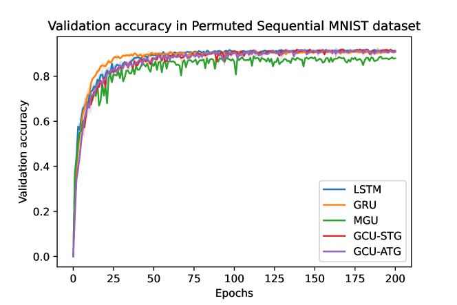
Figure 8: Validation accuracy in the permuted sequential MNIST dataset. GCUs demonstrate a sligtly better validation accuracy when compared to GRUs and LSTMs in this challenging task.

To answer this question we conduct experiments on a wide range of time-series modeling applications, including the classification of activities based on irregularly sampled localization data, IMDB movie reviews, and permuted sequential MNIST task. To achieve a somewhat similar number of parameters, we use 64 cells for GCUs, and 100 cells for the other. The total number of parameters in a model also depends on the number of inputs and outputs of the tasks considered. Finally, we also conduct experiments in a relatively complex and high-dimensional, image-based regression task for lane keeping in autonomous vehicles.

5.1 Localization Data for Person Activity

The localization data for the Person Activity dataset given in Vidulin et al. (2010), captures the recordings of five individuals, which engage in various activities. Each person wore four sensors at the left and the right ankle, at the chest, and at the belt, while repeating the same activity five times.

The associated task, is to classify their activity based on the irregularly sampled time-series. This task is a classification problem, adapted from (Lechner & Hasani, 2020).

In Table 1 we present the experimental results for the accuracy of the classification, for LSTMs, GRUs, MGUs, and GCUs. The experiments for the GCUs were done with both the asymmetric sigmoidal TG (GCU-ATG), and the symmetric, difference of sigmoids TG (GCU-STG). As one can see from the table, both GCUs considerably outperformed the traditional gated RNNs. In particular, the GCU-STG performed best, achieving an accuracy of 84.99% being slightly better than the GCU-ATG.

In Figure 6 we show the validation accuracy for the considered models. While the GCUs converge somewhat slower, they both surpass the other models after 100 epochs.

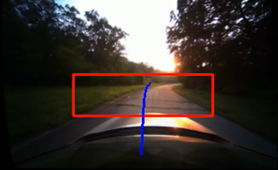
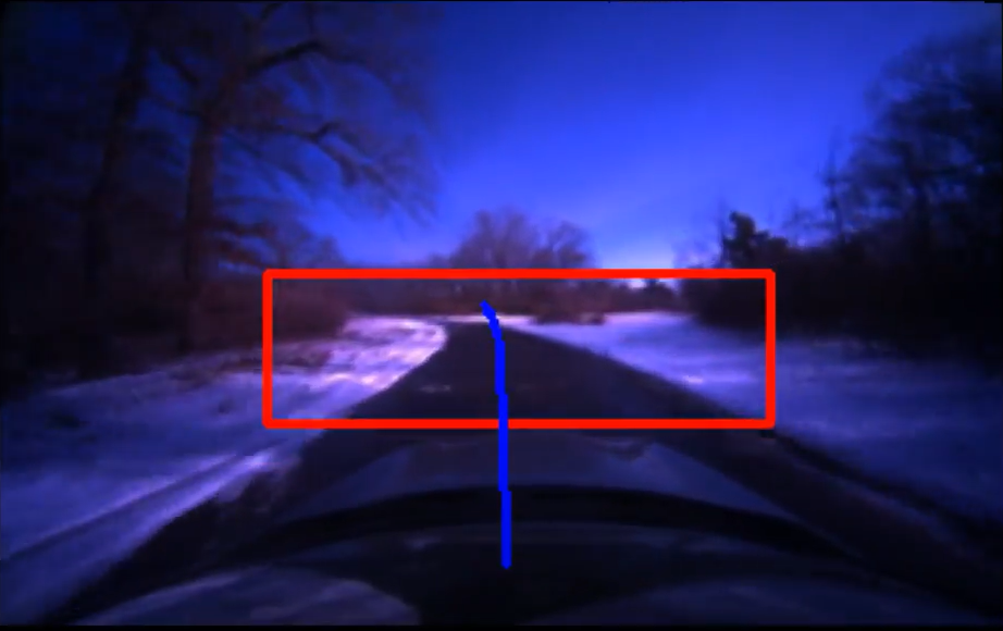
Figure 9: Lane-Keeping task. Red rectangle indicates the input and blue line shows the predicted steering angle of the network. Left is shown summer condition, and right is shown winter condition.

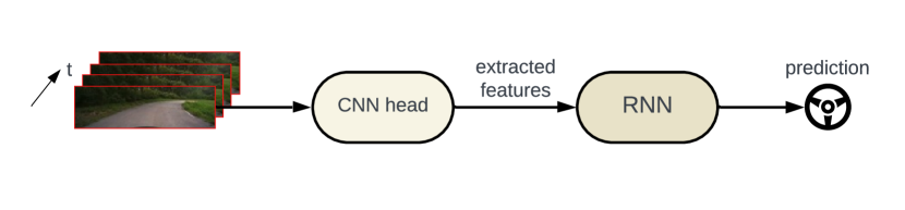
Figure 10: The overall network architecture for the Lane-Keeping task. The CNN head extracts the input features of a video stream. They are passed to the recurrent policy, responsible for steering.

5.2 IMDB Movie Sentiment Classification

The IMDB movie-review sentiment classification dataset, also known as the Large Movie Review Dataset (Maas et al., 2011), is designed for binary sentiment classification. It includes 25,000 movie reviews for both training and testing. Each review is labeled with a positive or negative sentiment.

In Table 2, we present our experimental results, comparing the accuracy the LSTMs, GRUs, MGUs, and GCUs. While the GCU-STG achieved a performance which was comparable to the one of the traditional RNNs, the GCU-ATG had the best performance, by achieving an accuracy of 87%.

In Figure 7, we show the validation accuracy for the considered models. GCU-ATG achieves the highest accuracy after only 5 epochs, even though this decreases a bit over time.

5.3 Permuted Sequential MNIST

The Permuted Sequential MNIST dataset, is a variant of the MNIST digits classification dataset, designed to evaluate recurrent neural networks, adapted from Le et al. (2015). In this task, the 784 pixels (originally $28{\times}28$ images) of digits are presented sequentially to the network. The challenge lies in predicting the digit category only after all pixels are observed. This task tests the network’s ability to handle long-range dependencies. To make the task more complex, a fixed random permutation of the pixels is applied.

In Table 3, we present our experimental results, comparing the accuracy the LSTMs, GRUs, MGUs, and GCUs. As before, both GCUs surpass the accuracy of the other models. In particular, the GCU-STG achieves the best results.

In Figure 8, we show the validation accuracy for the considered models. The GCUs achieve a slightly better validation accuracy when compared to GRUs and LSTMs on this task.

5.4 Lane-Keeping Task

In the Lane-Keeping Task, the agent is provided with the front-camera input, consisting of $48{\times}160$ pixels of RGB channels, and required to autonomously navigate and maintain its position within the road, by predicting its curvature. The predicted road curvature corresponds to the steering action necessary for lane-keeping, and holds the advantage of being vehicle-independent, as the actual steering angle depends on the type of car used. The dataset for this task is obtained from human-driving recordings, captured under various weather conditions (Lechner et al., 2022), as illustrated in Figure 9.

Table 4: Accuracy results for the Lane-Keeping task, averaged over 3 seeds. The total number of parameters of the recurrent part is 8k, where the number of neurons used for LSTMs, GRUs, MGUs, GCU-STG, and GCU-ATG are 23, 28, 38, 19, and 19 respectively.

Model	Validation Loss	Weighted Val. Loss
LSTM	$\mathbf{0.139\pm 0.008}$	$0.013\pm 0.001$
GRU	$0.145\pm 0.006$	$0.013\pm 0.001$
MGU	$\mathbf{0.139\pm 0.007}$	$0.012\pm 0.001$
GCU-STG	$0.142\pm 0.004$	$\mathbf{0.011\pm 0.001}$
GCU-ATG	$0.154\pm 0.005$	$\mathbf{0.010\pm 0.0003}$

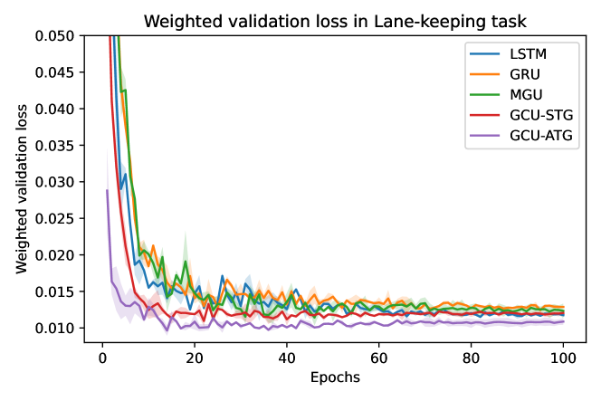
Figure 11: Weighted validation loss for the Lane-Keeping regression task. GCUs converge faster and to lower weighted validation losses. The GCU with asymmetric time gate performs best, by essentially converging after only $10$ epochs, and to a loss of $0.01$.

The network architecture contains a CNN-head for extracting features from the camera input that we feed into the gated recurrent models for the sequential-regression prediction. This network architecture is illustrated in Figure 10. This setup is adapted from Farsang et al. (2023).

In Table 4, we report the losses of the models on the Lane-Keeping task. As before, both GCUs obtain comparable validation losses, with GCU-ATG achieving the best weighted-validation loss, which is arguably the more important one.

In Figure 11 we show the weighted validation loss for the considered models. Both GCUs converge faster and to a lower loss, compared to the traditionally used gated RNNs.

6 Conclusion

In this paper we connected neuro-science to gated RNNs for the first time, by introducing GCUs. The latter constitute the first formal derivation of a gated RNN, from saturated Electrical Equivalent Circuits (EECs), which describe the behavior of biological neurons with chemical synapses as a set of neural ordinary differential equations (Neural ODEs).

GCUs make the integration of the Neural ODEs associated to the saturated EECs finally practicable, with an excellent convergence and accuracy, by introducing a time gate (TG), learning the optimal time step for every neuron and every integration step. In GCUs we also identify the forget gate (FG) with the liquid time constant of the GCUs, as this determines the rate of forgetting the previous state in EECs.

By identifying the FG of GCUs with a particular gate in the commonly-used gated RNNs, we are also able to shed new light into the inner workings of these RNNs, by showing that they can all be understood as instances of Neural ODEs. These ODE instances posses a trivial FG, as their time constant is 1. However, they use a more sophisticated mechanism (one more gate) to adjust the state in the update.

Finally, we experimentally showed that GCUs perform as well or better than their gated recurrent counterparts, on a comprehensive set of tasks used to assess gated RNNs. For future work, there might still be a better way of learning the TG, which would make GCUs even more powerful. From a wider perspective, this neuroscience-based gated RNN can also serve as a new computational building block for more sophisticated networks, in challenging time-series problems.

Appendix A Experiment Details

A.1 Localization Data for Person Activity

Considering that this is an irregularly sampled dataset, including separate extra timestep information per input, traditionally used gated units need further modification when dealing with this task. For LSTMs, GRUs and MGUs we concatenate this timestep information directly with the input features. This time step is used as the $\Delta_{t}$ value of the Time Gate in GCUs. LSTM, GRU and MGU networks contain 100 units, while GCUs have 100 units.

Table 5: Hyperparameters of the Localization Data for Person Activity experiment.

Variable	Value
Learning rate	$10^{-3}$
Optimizer	RMSprop (Tieleman & Hinton, 2017)
Batch size	$128$
Training sequence length	$32$
Epochs	$100$

A.2 IMDB Movie Sentiment Classification

In the IMDB review dataset we keep the 20,000 most frequent words and truncate the sequences up to 256 characters. Token embeddings of size 64 are used. LSTM, GRU and MGU have 100 units, while GCU variants have 100 cells in the networks.

Table 6: Hyperparameters of the IMDB Movie Sentiment Classification task.

Variable	Value
Learning rate	$10^{-3}$
Optimizer	Adam (Kingma & Ba, 2017)
Batch size	$64$
Training sequence length	$256$
Epochs	$30$

A.3 Permuted Sequential MNIST

As in the other classification tasks, traditionally used gated networks, such as LSTMs, GRUs and MGUs, have 100 units, and the proposed GCUs contain 64 units.

Table 7: Hyperparameters of the Permuted Sequential MNIST experiment.

Variable	Value
Learning rate	$10^{-3}$
Optimizer	RMSprop (Tieleman & Hinton, 2017)
Batch size	$64$
Training sequence length	$784$
Epochs	$200$

During the training of this task, the computed loss values of MGUs became NaNs in 2 out of the 3 runs in the middle of the experiments. Thus, for plotting the validation accuracy in Figure 8, we included only one full successful run for them.

A.4 Lane-Keeping Task

For the Lane-Keeping task, we built up the networks from 23, 28, 38 and 19 units of LSTMs, GRUs, MGUs and GCUs, respectively.

Table 8: Layers in the convolutional head in the Lane-Keeping task. Settings are adapted from Farsang et al. (2023).

Layer Type	Settings
Input	Input shape: (48, 160, 3)
Image-Norm.	Mean: 0, Variance: 1
Conv2D	Filters: 24, Kernel size: 5, Stride: 2, Activ.: ReLU
Conv2D	Filters: 36, Kernel size: 5, Stride: 1, Activ.: ReLU
MaxPool2D	Pool size: 2, Stride: 2
Conv2D	Filters: 48, Kernel size: 3, Stride: 1, Activ.: ReLU
MaxPool2D	Pool size: 2, Stride: 2
Conv2D	Filters: 64, Kernel size: 3, Stride: 1, Activ.: ReLU
MaxPool2D	Pool size: 2, Stride: 2
Conv2D	Filters: 64, Kernel size: 3, Stride: 1, Activ.: ReLU
Flatten	-
Dense	Units: 64

Table 9: Hyperparameters of the Lane-Keeping experiment.

Variable	Value
Learning rate	cosine decay, $5\cdot 10^{-4}$
Optimizer	AdamW (Loshchilov & Hutter, 2017)
Weight decay	$10^{-6}$
Batch size	$32$
Training sequence length	$32$
Epochs	$100$

References

- Cho et al. (2014) Cho, K., Van Merriënboer, B., Gulcehre, C., Bahdanau, D., Bougares, F., Schwenk, H., and Bengio, Y. Learning phrase representations using rnn encoder-decoder for statistical machine translation. arXiv preprint arXiv:1406.1078, 2014.
- Farsang et al. (2023) Farsang, M., Lechner, M., Lung, D., Hasani, R., Rus, D., and Grosu, R. Learning with chemical versus electrical synapses – does it make a difference? arXiv preprint arXiv:2401.08602, 2023.
- Greff et al. (2016) Greff, K., Srivastava, R. K., Koutník, J., Steunebrink, B. R., and Schmidhuber, J. Lstm: A search space odyssey. IEEE transactions on neural networks and learning systems, 28(10):2222–2232, 2016.
- Hasani et al. (2020) Hasani, R. M., Lechner, M., Amini, A., Rus, D., and Grosu, R. Liquid time-constant networks. In AAAI Conference on Artificial Intelligence, 2020.
- Hochreiter & Schmidhuber (1997) Hochreiter, S. and Schmidhuber, J. Long short-term memory. Neural Comput., 9(8):1735–1780, nov 1997. ISSN 0899-7667. doi: 10.1162/neco.1997.9.8.1735. URL https://doi.org/10.1162/neco.1997.9.8.1735.
- Józefowicz et al. (2015) Józefowicz, R., Zaremba, W., and Sutskever, I. An empirical exploration of recurrent network architectures. In International Conference on Machine Learning, 2015. URL https://api.semanticscholar.org/CorpusID:9668607.
- Kandel et al. (2000) Kandel, E. R., Schwartz, J. H., Jessell, T. M., Siegelbaum, S., Hudspeth, A. J., Mack, S., et al. Principles of neural science, volume 4. McGraw-hill New York, 2000.
- Kingma & Ba (2017) Kingma, D. P. and Ba, J. Adam: A method for stochastic optimization, 2017.
- Le et al. (2015) Le, Q. V., Jaitly, N., and Hinton, G. E. A simple way to initialize recurrent networks of rectified linear units. arXiv preprint arXiv:1504.00941, 2015.
- Lechner & Hasani (2020) Lechner, M. and Hasani, R. Learning long-term dependencies in irregularly-sampled time series. arXiv preprint arXiv:2006.04418, 2020.
- Lechner et al. (2019) Lechner, M., Hasani, R., Zimmer, M., Henzinger, T. A., and Grosu, R. Designing worm-inspired neural networks for interpretable robotic control. In 2019 International Conference on Robotics and Automation (ICRA), pp. 87–94, 2019. doi: 10.1109/ICRA.2019.8793840.
- Lechner et al. (2020) Lechner, M., Hasani, R. M., Amini, A., Henzinger, T. A., Rus, D., and Grosu, R. Neural circuit policies enabling auditable autonomy. Nature Machine Intelligence, 2:642–652, 2020.
- Lechner et al. (2022) Lechner, M., Hasani, R., Amini, A., Wang, T.-H., Henzinger, T. A., and Rus, D. Are all vision models created equal? a study of the open-loop to closed-loop causality gap. arXiv preprint arXiv:2210.04303, 2022.
- Loshchilov & Hutter (2017) Loshchilov, I. and Hutter, F. Fixing weight decay regularization in adam. ArXiv, abs/1711.05101, 2017. URL https://api.semanticscholar.org/CorpusID:3312944.
- Maas et al. (2011) Maas, A. L., Daly, R. E., Pham, P. T., Huang, D., Ng, A. Y., and Potts, C. Learning word vectors for sentiment analysis. In Lin, D., Matsumoto, Y., and Mihalcea, R. (eds.), Proceedings of the 49th Annual Meeting of the Association for Computational Linguistics: Human Language Technologies, pp. 142–150, Portland, Oregon, USA, June 2011. Association for Computational Linguistics. URL https://aclanthology.org/P11-1015.
- Shampine & Witt (1995) Shampine, L. and Witt, A. A simple step size selection algorithm for ode codes. Journal of Computational and Applied Mathematics, 58(3):345–354, 1995. ISSN 0377-0427. doi: https://doi.org/10.1016/0377-0427(94)00007-N. URL https://www.sciencedirect.com/science/article/pii/037704279400007N.
- Tieleman & Hinton (2017) Tieleman, T. and Hinton, G. Divide the gradient by a running average of its recent magnitude. coursera: Neural networks for machine learning. Technical report, 2017.
- Vidulin et al. (2010) Vidulin, V., Lustrek, M., Kaluza, B., Piltaver, R., and Krivec, J. Localization Data for Person Activity. UCI Machine Learning Repository, 2010. DOI: https://doi.org/10.24432/C57G8X.
- Wicks et al. (1996) Wicks, S. R., Roehrig, C. J., and Rankin, C. H. A dynamic network simulation of the nematode tap withdrawal circuit: predictions concerning synaptic function using behavioral criteria. Journal of Neuroscience, 16(12):4017–4031, 1996.
- Zhou et al. (2016) Zhou, G.-B., Wu, J., Zhang, C.-L., and Zhou, Z.-H. Minimal gated unit for recurrent neural networks. International Journal of Automation and Computing, 13(3):226–234, 2016.