Using Sequential Runtime Distributions for the Parallel Speedup Prediction of SAT Local Search

Abstract

This paper presents a detailed analysis of the scalability and parallelization of local search algorithms for the Satisfiability problem. We propose a framework to estimate the parallel performance of a given algorithm by analyzing the runtime behavior of its sequential version. Indeed, by approximating the runtime distribution of the sequential process with statistical methods, the runtime behavior of the parallel process can be predicted by a model based on order statistics. We apply this approach to study the parallel performance of two SAT local search solvers, namely Sparrow and CCASAT, and compare the predicted performances to the results of an actual experimentation on parallel hardware up to 384 cores. We show that the model is accurate and predicts performance close to the empirical data. Moreover, as we study different types of instances (random and crafted), we observe that the local search solvers exhibit different behaviors and that their runtime distributions can be approximated by two types of distributions: exponential (shifted and non-shifted) and lognormal.

1 Introduction

Nowadays, SAT solvers are very effective to solve problems in a wide variety of domains ranging from software verification to computational biology and automated planning. Broadly speaking, there are two main categories of SAT solvers: complete and incomplete. Complete solvers combine tree-based search with unit propagation, conflict-clause learning, and intelligent backtracking. Incomplete solvers start with an initial assignment for the variables (usually random); then the solver iteratively moves in the search space until a given stopping criteria is met. These solvers are very good at tackling large and difficult (random) instances.

Research on parallel SAT solvers have been rapidly increasing in the last decade, thanks to the the development and increasing availability of parallel hardware, such as multi-core architectures, GPGPUs, grids, cloud systems, and massively parallel supercomputers. A well-known approach for parallel SAT solving is search-space splitting; it consists in dividing the problem space into several sub-spaces and exploring them in parallel. Another approach consists in building a parallel portfolio solver in which several algorithms compete and cooperate to solve a given problem instance. Motivated by the results of the recent SAT competitions, most researchers currently focus their attention on the development of parallel portfolios for multi-core architectures. The computational benefit of the parallel portfolio is observed in both capacity solving and speedup factor. Capacity solving, or Solution Count Ranking [Van Gelder (2011)], refers to the ability of improving the total number of solved instances within a given timelimit, while speedup refers to the ability of reducing the runtime (w.r.t. the sequential solver) to solve individual instances. Previous work has been mainly focused on studying the capacity solving of complete parallel SAT solvers, see [Martins et al. (2012)] for a recent survey.

Up to now, most parallel SAT solvers have been designed for multi-core machines or small clusters with a few tens of processors. A key question is therefore to know if these approaches could scale up to massively parallel systems, i.e., with thousands or tens of thousands of cores. To investigate this exiting new field of endeavor, we studied in this paper the parallel performance of several SAT solvers up to several hundreds of cores. Moreover, we propose a probabilistic model to estimate the parallel performance of local search algorithms for SAT, using a simple scheme for parallelization. By analyzing the sequential runtime, we can predict the parallel behavior and quantify the expected parallel speedup. More precisely, we first approximate the empirical sequential runtime distribution by a well-known statistical distribution (e.g. exponential or lognormal) and then derive the runtime distribution of the parallel version of the solver. Our model is related to order statistics, a rather new domain of statistics [David and Nagaraja (2003)], which is the statistics of sorted random draws. This makes it possible to predict the parallel runtime of a given algorithm for any number of cores.

The main contributions of this paper are as follows. First, we present the application of a statistical model to predict and evaluate the performance of parallel local search algorithms for SAT. Moreover, extensive experimental results (up to 384 cores) using state-of-the-art local search solvers showed that the predicted execution times and speedups accurately match the empirical data and performance. Second, we provide an understanding of the different speedups of parallel algorithms for SAT from a theoretical and empirical point of view for two different families of benchmarks.

This paper is organized as follows. After a brief presentation of parallel local search for SAT in Section 2, Section 3 describes the framework of runtime distributions and formally defines the probabilistic model used to predict the parallel performance of local search algorithms. Section 4 details extensive experimental results performed to evaluate the model. Section 5 presents concluding remarks and future research directions.

2 Parallel Local Search for SAT

Parallel implementation of local search methods for combinatorial problems has been studied since the early 1990s, when parallel machines started to become widely available [Pardalos et al. (1995), Verhoeven and Aarts (1995)]. Apart from domain-decomposition methods and population-based method (e.g., genetic algorithms), [Verhoeven and Aarts (1995)] distinguishes between single-walk and multi-walk methods for Local Search. Single-walk methods consist in using parallelism inside a single search process, e.g., for parallelizing the exploration of the neighborhood. Multi-walk methods (parallel execution of multi-start methods) consist in developing concurrent explorations of the search space, either independently or cooperatively with some communication between processes.

It is now currently admitted that an easy and effective manner to parallelize local search solvers consists in executing in parallel multiple copies of a given solvers with or without cooperation. The non-cooperative approach has been used in the past to solve SAT and MaxSAT instances. gNovelty+ [Pham and Gretton (2007)] executes multiple copies of gNovelty without cooperation until a solution is obtained or a given timeout is reached; and [Pardalos et al. (1996)] executes multiple copies of GRASP until an assignment which satisfies a given number of clauses is obtained. Strategies to exploit cooperation between parallel SAT local search solvers have been studied in [Arbelaez and Hamadi (2011)] in the context of multi-core architectures with shared memory and in [Arbelaez and Codognet (2012)] in massively parallel systems with distributed memory.

The analysis proposed in this paper for predicting performance on massively parallel systems is set in the framework of independent multi-walk parallelism, as it seems to be the most promising way to deal with large-scale parallelism. Cooperative algorithms might perform well on shared-memory machines with a few tens of cores, but are difficult to extend efficiently to distributed hardware.

3 Analysis using runtime distributions

Most papers on the performance of stochastic local search algorithms focus on the average execution time in order to measure the performance of both sequential and parallel executions. However, a more detailed analysis of the runtime behavior could be done by looking at the execution time of the algorithm (e.g., cpu-time or number of iterations) as a random variable and performing a statistical analysis of its probability distribution.

3.1 Approximating Runtime Behaviors

The notion of runtime distribution has been introduced by [Hoos and Stützle (1998)] to characterize the cumulative distribution function of the execution time of stochastic algorithms. Indeed, Stochastic Local Search [Hoos and Stütze (2005)] can be considered in the larger framework of Las Vegas algorithms, introduced a few decades ago by [Babai (1979)], i.e. randomized algorithms whose runtime might vary from one execution to another, even with the same input. It has been applied to study random 3-SAT problems with the Walk-SAT solver [Hoos and Stützle (1999)], combinatorial optimization problems with the GRASP metaheuristics [Aiex et al. (2002)] and path-planning problems with state-graph search algorithms (e.g., A*) [Munoz et al. (2012)]. The study of the runtime behavior of parallel extensions of Las Vegas algorithm in the framework of (independent) multi-walk processes has been proposed by [Truchet et al. (2013)], which presents a model for predicting the parallel performance of a given Las Vegas algorithm by the statistical analysis of its sequential version. The runtime distribution has also been used to define optimal restart strategies in sequential and parallel algorithms in [Shylo et al. (2011)] and to provide bounds on the parallel expectation by [Luby et al. (1993)]. However, in this paper we are using it to predict the parallel speedup in a multi-walk scheme from the study of the initial sequential problem distribution.

Indeed, since [Verhoeven and Aarts (1995), Verhoeven (1996)], it is believed that combinatorial problems can enjoy a linear speedup when implemented in parallel by independent multi-walks. However, this has been proven only under the assumption that the probability of finding a solution in a given time $t$ follows an exponential law, that is, if the runtime behavior follows a (non-shifted) exponential distribution. This behavior has been conjectured for SAT local search solvers in [Hoos and Stützle (1999)], and confirmed experimentally for the GRASP metaheuristics solver on some other classical combinatorial problems [Aiex et al. (2002)]. The latter authors have also developed, in the context of combinatorial optimization, a simple tool (tttplot) to study the adequation of a given runtime behavior with an exponential distribution [Aiex et al. (2007)]. The classical explanation for an exponential runtime behavior is the fact that the solutions are uniformly distributed in the search space, (and not regrouped in solution clusters [Maneva and Sinclair (2008)]) and that the random search algorithm is able to sample the search space in a uniform manner. However, [Truchet et al. (2013)] shows that the runtime distribution of local search solvers for combinatorial problems can be not only exponential but also sometimes lognormal or shifted exponential, in which cases the parallel speedup cannot be linear and is asymptotically bounded. Indeed, not all combinatorial problems show a perfect exponential behavior, and we will see in this paper how this applies to SAT.

3.2 Min Distribution and Parallel Speed-up

A general statistical model for studying the performance of Las Vegas algorithms and predicting the parallel performance of their parallel multi-walk extensions has been recently proposed in [Truchet et al. (2013)]. We will now present a brief summary of this model, which will be used in the rest of the paper to study the behavior of two local search solvers on a variety of SAT instances.

Let $Y$ be the runtime of a Local Search algorithm on a given problem instance. It can be considered as a random variable with values in $\mathbb{N}$ (number of iterations), or in $\mathbb{Q}$ (cpu-time). In general, it is more convenient to consider distributions with values in $\mathbb{R}$ because calculations are easier. $Y$ can be studied through its cumulative distribution, which is by definition, the function $\mathcal{F}_{Y}$ s.t. $\mathcal{F}_{Y}(x)=Pr(Y\leq x)$. By definition, the distribution of $Y$ is the derivative of $\mathcal{F}_{Y}$: $f_{Y}=\mathcal{F}_{Y}^{\prime}$. The expectation of $Y$ is defined as $\mathbb{E}[Y]=\int_{0}^{\infty}tf_{Y}(t)dt$

Assume that $n$ copies of the base algorithm are running in parallel on $n$ cores. The first process finding a solution kills all others, and the overall parallel algorithm terminates. The $i$-th process corresponds to a draw of a random variable $X_{i}$, following the distribution $f_{Y}$. The variables $X_{i}$ are thus independent and identically distributed (i.i.d.). The computation time of the whole parallel process is also a random variable, let $Z^{(n)}$, with a distribution $f_{Z^{(n)}}$ that depends both on $n$ and on $f_{Y}$. Since all the $X_{i}$ are i.i.d., the cumulative distribution $\mathcal{F}_{Z^{(n)}}$ and the distribution $f_{Z^{(n)}}$ can be computed as follows:

$$\begin{array}[]{ccccc}\@add@centering\centering\mathcal{F}_{Z^{(n)}}&=&Pr(Z^{(n)}\leq x)&=&\leavevmode\nobreak\ \leavevmode\nobreak\ Pr(\exists i\in\{1...n\},X_{i}\leq x)\\ &=&\leavevmode\nobreak\ \leavevmode\nobreak\ 1-Pr(\forall i\in\{1...n\},X_{i}>x)\nobreak\leavevmode\nobreak\leavevmode&=&1-\left(1-\mathcal{F}_{Y}(x)\right)^{n}\\ f_{Z^{(n)}}&=&\lx@intercol\left(1-(1-\mathcal{F}_{Y}\right)^{n})^{\prime}=nf_{Y}(1-\mathcal{F}_{Y})^{n-1}\hfil\lx@intercol\\ \end{array}$$

Thus, knowing the distribution for the base algorithm $Y$, one can calculate the distribution for $Z^{(n)}$. The formula shows that the parallel algorithm favors short runs, by killing slower processes. Thus, compared to the distribution of $Y$, the distribution of $Z^{(n)}$ moves toward the origin and is more peaked.

We can also compute the expectation $\mathbb{E}[Z^{(n)}]$ for the parallel process, from which we derive the expected speed-up $\mathcal{G}_{n}$ of the parallel algorithm versus the sequential one:

$$\mathbb{E}[Z^{(n)}] = n\int_{0}^{\infty}tf_{Y}(t)(1-\mathcal{F}_{Y}(t))^{n-1}dt$$

$$\mathcal{G}_{n} = \mathbb{E}[Y]/\mathbb{E}[Z^{(n)}]$$

Again, no explicit general formula can be computed and the expression of the speed-up will depend on the distribution of $Y$. We will thus study in the following different specific distributions. This computation of the speed-up is actually related to a field of statistics called order statistics, see [David and Nagaraja (2003)] for a detailed presentation. Order statistics are the statistics of sorted random draws. For instance, the first order statistics of a distribution is its minimal value. For predicting the speedup, we are indeed interested in computing the expectation of the distribution of the minimum draw. As the above formula suggests, this may lead to heavy calculations, but recent studies such as [Nadarajah (2008)] give explicit formulas defining this quantity for several classical probability distributions.

3.3 Exponential and Lognormal Distributions

Assume that $Y$ has a shifted exponential distribution, as would be the case for an ideal randomized algorithm. The minimum distribution can be computed by a direct integration: $f_{Y}(t)$=$\lambda e^{-\lambda(t-x_{0})}$ for t$>$ 0; $\mathbb{E}[Y]$=$x_{0}+1/\lambda$; and $f_{Z^{(n)}}(t)$=$n$$\lambda e^{-n\lambda(t-x_{0})}$ for $t>0$.

In case of a non-shifted exponential, $x_{0}=0$ and the speed-up is thus equal to the number of cores $n$, up to infinity. This case has already been studied by [Verhoeven and Aarts (1995)]. However for $x_{0}>0$, the speed-up admits a finite limit, even when $n$ tends to infinity, which is $\frac{x_{0}+\frac{1}{\lambda}}{x_{0}}=1+\frac{1}{x_{0}\lambda}$. The closer to zero $x_{0}$ is, the higher the limit.

Other distributions can be considered, depending on the behavior of the base algorithm. We will study the case of a lognormal distribution, which is the log of a gaussian distribution, because it will appear in the following experiments for some instances. The lognormal distribution has two parameters, the mean $\mu$ and the standard deviation $\sigma$. Formally, a (non-shifted) lognormal distribution is defined as: $f_{Y}(t)=\frac{e^{-\frac{(-\mu+log(t))^{2}}{2\sigma^{2}}}}{\sqrt{2\pi}(t)\sigma}$

The formulas for the distribution of $Z^{(n)}$, its expectation and the theoretical speed-up are quite complicated to compute, but [Nadarajah (2008)] gives an explicit formula for all the moments of lognormal order statistics with only a numerical integration step, from which we can derive a computation of the speed-up. As for the shifted exponential, it can be shown that the speed-up curve of the lognormal distribution admits a finite limit.

4 Experimental Settings and Results

This section describes the benchmark instances used for tests, and we focus our attention on two well-known problem families: random and crafted instances. Moreover, we consider the two best local search solvers from the previous SAT competition: CCASAT [Cai et al. (2012)] and Sparrow [Balint and Fröhlich (2010)]. Both solvers were used with their default parameters and with a timeout of 3 hours for each experiments. All the experiments were performed on the Grid’5000 platform, the French national grid for research. We used a 44-node cluster with 24 cores (2 AMD Opteron 6164 HE processors at 1.7 Ghz) and 44 GB of RAM per node. We experimented with 10 random instances (6 around the phase transition) and 10 crafted instances (see the appendix for a complete presentation of the instances).

In order to obtain the empirical data for the theoretical distribution (predicted by our model from the sequential runtime distribution), we performed 500 runs of the sequential algorithm. The Mathematica software [Wolfram (2003)], version 8.0, was used to estimate the parameters of the theoretical distributions and to integrate numerically the formulas of the lognormal distribution. In order to evaluate the accuracy of the learned statistical model, we performed 50 runs of the multi-walk parallel algorithms. The empirical speedup for a given parallel algorithm is calculated against the mean performance of its sequential version as follows: $Speedup=\frac{\textit{Mean}(Solver\leavevmode\nobreak\ on\leavevmode\nobreak\ 1\textit{ core})}{\textit{Mean}(Solver\leavevmode\nobreak\ on\leavevmode\nobreak\ \textit{N cores})}$

4.1 Experimental results

In this section, we start by presenting the empirical and estimated results for random and crafted instances; then we present a general analysis of the results.

We start our analysis with Table 1, which presents initial statistics for the sequential version of Sparrow and CCASAT. We present the minimum, maximum, and mean runtime values, as well as the outcome of the Kolmogorov-Smirnov (KS) test for two types of distributions: shifted exponential and lognormal. In the following tables, bold numbers indicate the distribution chosen to predict the performance of a given solver.

Instance	Alg	Min	Max	Mean	p-value
					Shifted exp. dist.	Lognormal dist.
Rand-1	Sparrow	98.0	4860.0	793.9	5.6$\cdot 10^{-19}$	0.76
	CCASAT	103.6	1340.1	458.5	8.4$\cdot 10^{-55}$	0.96
Rand-2	Sparrow	91.8	5447.0	1007.5	1.8$\cdot 10^{-20}$	0.91
	CCASAT	108.8	1652.9	497.9	5.1$\cdot 10^{-58}$	0.71
Rand-3	Sparrow	104.8	3693.7	797.0	2.9$\cdot 10^{-26}$	0.64
	CCASAT	126.48	1125.4	359.6	2.3$\cdot 10^{-108}$	0.90
Rand-4	Sparrow	162.4	3037.8	781.5	1.6$\cdot 10^{-38}$	0.03
	CCASAT	132.5	980.9	382.0	1.5$\cdot 10^{-117}$	0.92
Rand-5	Sparrow	164.0	7946.3	952.4	1.8$\cdot 10^{-31}$	0.16
	CCASAT	158.6	1177.9	403.1	5.1$\cdot 10^{-134}$	0.20
Rand-6	Sparrow	142.0	4955.8	763.5	1.6$\cdot 10^{-31}$	0.64
	CCASAT	142.9	890.9	354.1	9.6$\cdot 10^{-137}$	0.46
Rand-7	Sparrow	35.5	10637.4	3464.2	0.01	1.5$\cdot 10^{-4}$
	CCASAT	61.6	6419.1	1801.0	1.0$\cdot 10^{-5}$	0.13
Rand-8	Sparrow	23.2	10738.0	3412.9	0.05	4.7$\cdot 10^{-4}$
	CCASAT	35.9	10443.7	2007.6	0.50	0.03
Rand-9	Sparrow	6.8	5935.8	1028.2	0.23	3.7$\cdot 10^{-3}$
	CCASAT	18.1	2830.4	476.8	7.0$\cdot 10^{-3}$	0.03
Rand-10	Sparrow	19.0	10800.0	1726.3	0.65	0.15
	CCASAT	19.8	4854.5	758.4	7.6$\cdot 10^{-10}$	0.18

Table 1: Performance of sequential algorithms on random instances

The KS test compares a set of empirical measures to a given theoretical distribution. Its outcome is a p-value, indicating how likely it is that the measures admits the theoretical distribution. The classical threshold for the p-value is 0.05. For greater p-values, the KS test succeeds (more precisely, the null hypothesis is not rejected), and the empirical distribution can be approximated by the theoretical one with good confidence.

The results presented in this table are consistent with the results of the previous SAT competition (random category) where CCASAT greatly outperformed Sparrow. For this set of instances, we choose the shifted exponential distribution in lieu of the exponential distribution as the Min runtime value for the reference solvers is not negligible compared to its mean value across 500 executions (about 100 times smaller in the best case).

As can be seen from the table, both solvers report a tendency which indicates that the empirical data for instances around the phase transition are better approximated by a lognormal distribution; all these instances pass the KS test with a confidence level (p-value) above 0.05, except for Sparrow on rand-4.

For instances outside the phase transition, Sparrow reports enough statistical evidence to infer that the shifted exponential distribution fits better the empirical data. For CCASAT, 3 out of 4 instances outside the phase transition are better characterized with a lognormal distribution and the remaining instance pass the KS test for the shifted exponential distribution.

Instance		Sparrow - Runtime on $k$ cores				CCASAT - Runtime on $k$ cores
		48	96	192	384	48	96	192	384
Rand-1	Actual	163.8	140.4	125.2	113.7	160.0	143.0	122.8	112.0
	Predicted	133.8	110.5	92.7	78.8	137.7	120.6	106.7	95.3
Rand-2	Actual	213.2	191.4	166.2	142.5	186.8	169.3	159.3	142.8
	Predicted	183.5	152.8	129.2	110.6	153.4	134.7	119.6	107.1
Rand-3	Actual	175.9	151.2	135.8	123.5	166.7	155.6	143.5	132.2
	Predicted	183.5	152.8	129.2	110.6	153.4	134.7	119.6	107.1
Rand-4	Actual	202.3	179.2	159.5	141.8	193.1	176.0	169.4	158.7
	Predicted	175.7	149.5	128.9	112.4	170.6	155.9	143.5	132.8
Rand-5	Actual	219.6	201.0	182.5	161.9	212.2	191.3	176.8	165.8
	Predicted	185.0	155.3	132.3	114.0	179.8	164.3	151.2	140.0
Rand-6	Actual	185.5	167.1	150.3	137.5	190.9	179.3	168.4	153.4
	Predicted	158.3	133.6	114.4	99.1	160.6	147.0	135.4	125.6
Rand-7	Actual	151.2	102.7	63.8	51.1	22.9	33.7	54.3	67.8
	Predicted	195.8	143.0	107.3	82.3	182.8	142.6	113.7	92.2
Rand-8	Actual	126.6	81.9	51.1	30.9	131.8	83.9	64.8	39.7
	Predicted	93.8	58.5	40.8	32.0	76.9	56.4	46.1	41.0
Rand-9	Actual	33.9	18.4	13.1	9.0	45.0	31.0	22.7	16.3
	Predicted	28.1	17.4	12.1	9.4	38.5	29.4	23.0	18.3
Rand-10	Actual	63.4	48.9	40.7	30.9	113.8	94.7	72.9	54.2
	Predicted	54.6	36.8	27.9	23.4	105.6	85.3	70.2	58.6

Table 2: Runtimes for random instances up to 384 cores

Let’s now look at the parallel performance of the solvers. Table 2 (resp. Table 3) shows the empirical and predicted runtime (resp. speedup) for both Sparrow and CCASAT on all instances using 48, 96, 192, and 384 cores. In Table 3, we observe an important difference in the speedup factor between the two solvers which suggest that in general Sparrow scales better than CCASAT.

Instance		Sparrow - Speedup on $k$ cores				CCASAT - Speedup on $k$ cores
		48	96	192	384	48	96	192	384
Rand-1	Actual	4.8	5.6	6.3	6.9	2.8	3.2	3.7	4.0
	Predicted	5.9	7.1	8.5	10.0	3.3	3.8	4.3	4.8
Rand-2	Actual	4.7	5.2	6.0	7.0	2.6	2.9	3.1	3.4
	Predicted	5.4	6.5	7.7	9.0	3.2	3.6	4.1	4.6
Rand-3	Actual	4.5	5.2	5.8	6.4	2.1	2.3	2.5	2.7
	Predicted	5.4	6.5	7.7	9.0	3.2	3.6	4.1	4.6
Rand-4	Actual	3.8	4.3	4.8	5.5	1.9	2.1	2.2	2.4
	Predicted	4.4	5.1	6.0	6.9	2.2	2.4	2.6	2.8
Rand-5	Actual	4.3	4.7	5.2	5.8	1.9	2.1	2.2	2.4
	Predicted	5.0	6.0	7.0	8.1	2.2	2.4	2.6	2.8
Rand-6	Actual	4.1	4.5	5.0	5.5	1.8	1.9	2.1	2.3
	Predicted	4.7	5.6	6.6	7.6	2.2	2.4	2.6	2.8
Rand-7	Actual	22.9	33.7	54.3	67.8	9.5	13.7	18.5	22.7
	Predicted	32.3	48.5	64.8	77.8	10.5	13.4	16.9	20.8
Rand-8	Actual	26.9	41.7	66.8	110.6	15.2	23.9	30.9	50.5
	Predicted	36.3	58.3	83.5	106.5	26.0	35.5	43.4	48.9
Rand-9	Actual	30.3	55.8	78.1	114.2	10.5	15.3	20.9	29.1
	Predicted	36.5	58.8	84.6	108.3	13.2	17.3	22.2	27.9
Rand-10	Actual	27.2	35.2	42.3	55.7	6.6	8.0	10.3	13.9
	Predicted	31.6	46.8	61.7	73.4	7.3	9.1	11.1	13.3

Table 3: Speedup for random instances up to 384 cores

Figure 1 shows a performance summary of the reference solvers to tackle an instance on the phase transition (rand-4) and another instance outside the phase transition (rand-7). The y-axis gives the probability ($Pr(Y\leq x)$) of finding a solution in a time less or equal to $x$ and the x-axis gives the runtime in seconds. From now on, in all figures ‘Emp’ stands for Empirical distribution, ‘LN’ stands for lognormal distribution, and ‘SExp’ stands for shifted exponential distribution. As expected CCASAT dominates the performance on one core. For example to solve rand-4, CCASAT reports $Pr(\textit{Y}\leq\textit{16-mins})$ $\approx$ 1.0, while Sparrow reports $Pr(\textit{Y}\leq\textit{16-mins})$ $\approx$ 0.75. Figures 1(c) and 1(f) show that for CCASAT increasing the number of cores does not significantly improve the solving time. Consequently, Sparrow becomes more effective for a large number of cores. Therefore, Figures 1(b) and 1(e) show that Sparrow is better than CCASAT when using 384 cores. Interestingly, the same pattern is observed for other random instances (see Table 2).

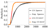
(a) Empirical CDF vs. theoretical CDF (rand-4)

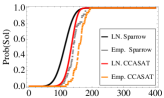
(b) Empirical CDF vs. predicted CDF using 384 cores (rand-4)

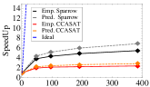
(c) Speedup (rand-4)

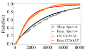
(d) Empirical CDF vs. theoretical CDF (rand-7)

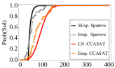
(e) Empirical CDF vs. predicted CDF using 384 cores (rand-7)

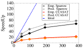
(f) Speedup (rand-7)

Figure 1: Performance summary to solve rand-4 and rand-7

To illustrate the power of the predicted model, in Figure 1(c) we present the predicted and empirical speedup curves for CCASAT and Sparrow. Here it can be observed that in both cases the predicted curve follows the same shape as the empirical one. Moreover, It is also important to note that the speedup factor of the reference solvers for this problem family is far from linear (ideal), a phenomenon described by the predicted model.

Finally, it can also be observed that random instances around the phase transition exhibit a lower speedup factor than the remaining random instances. For instance, the best empirical speedup factor obtained for instances in the phase transition is 7.0 for Sparrow and 3.4 for CCASAT; and the best speedup factor obtained for instances outside the phase transition is 114.2 for Sparrow and 50.5 for CCASAT.

Let’s switch our attention now to crafted instances, for which we have to treat differently CCASAT and Sparrow. For CCASAT, we were unable to find a theoretical distribution which fits the empirical data. It should be also noticed that CCASAT has been mainly designed and tuned to handle random instances. Let us look for instance at Figure 2(a), which depicts the cumulative runtime distribution of CCASAT to solve Crafted-1 using the two reference distributions detailed in this paper (lognormal and exponential) and two extra distributions (Weibull and beta-prime). None of the theoretical distributions seems to be a good approximation of the empirical data. More precisely, the KS test reported a p-value of 2.7$\cdot 10^{-7}$ (lognormal); 7.0$\cdot 10^{-24}$ (exponential); 2.4$\cdot 10^{-6}$ (Weibull); and 6.9$\cdot 10^{-15}$ (beta-prime). Therefore, none of the theoretical distributions pass KS test with a high-enough p-value. We also experimented with other instances and observed a similar behavior.

Instance	Alg	Min	Max	Mean	p-value
					Exp. dist.	Lognormal dist.
Crafted-1	Sparrow	9.9	10800.0	3440.3	0.02	1.2$\cdot 10^{-4}$
Crafted-2	Sparrow	1.0	10800.0	2711.2	0.57	1.4$\cdot 10^{-4}$
Crafted-3	Sparrow	8.7	10800.0	3432.7	0.14	1.1$\cdot 10^{-3}$
Crafted-4	Sparrow	2.2	10800.0	2701.6	0.11	9.6$\cdot 10^{-3}$
Crafted-5	Sparrow	4.1	10800.0	1564.1	0.95	9.2$\cdot 10^{-4}$
Crafted-6	Sparrow	2.9	10800.0	3599.6	0.01	1.0$\cdot 10^{-5}$
Crafted-7	Sparrow	4.4	10800.0	3598.7	0.01	7.8$\cdot 10^{-6}$
Crafted-8	Sparrow	3.5	5456.0	972.046	0.67	0.17
Crafted-9	Sparrow	1.9	7876.5	1298.24	0.97	7.0$\cdot 10^{-3}$

Table 4: Sequential performance of Sparrow on crafted instances

For Sparrow on all crafted instances, the KS test shows a much better p-value for the exponential distribution than for the lognormal one, see Table 4. The confidence level is quite high for the instances Crafted-2,-3,-4,-5,-8,-9, with p-value up to 0.97, while the p-value is between 0.01 and 0.02 for Crafted-1,-6,-7. Also, as the minimum runtime is much smaller than the mean (at least 300 times smaller), we can approximate the empirical data by a non-shifted exponential distribution [Truchet et al. (2013)].

As can be seen in Table 5 the multi-walk parallel approach scales well for Sparrow on crafted instances as the number of cores increases. Indeed a nearly linear speedup is obtained for nearly all the instances. As expected, the speedup predicted by our model is optimal, and this result is consistent with those obtained in [Hoos and Stützle (1999)].

Instance		Runtime on $k$ cores				Speedup ok $k$ cores
		48	96	192	384	48	96	192	384
Crafted-1	Actual	97.7	43.7	19.1	9.8	35.1	78.6	179.6	349.8
	Predicted	71.6	35.8	17.9	8.9	48.0	96.0	192.0	384.0
Crafted-2	Actual	67.8	36.4	17.5	7.2	39.9	74.4	154.7	375.2
	Predicted	56.4	28.2	14.1	7.0	48.0	96.0	192.0	384.0
Crafted-3	Actual	94.8	49.3	23.2	11.9	36.1	69.6	147.6	286.1
	Predicted	71.5	35.7	17.8	8.9	48.0	96.0	192.0	384.0
Crafted-4	Actual	87.5	42.0	17.3	9.7	30.8	64.2	155.4	277.8
	Predicted	56.2	28.1	14.0	7.0	48.0	96.0	192.0	384.0
Crafted-5	Actual	33.7	15.1	7.6	4.2	46.3	103.2	204.1	371.6
	Predicted	32.5	16.2	8.1	4.0	48.0	96.0	192.0	384.0
Crafted-6	Actual	130.0	69.8	25.6	12.8	27.6	51.5	140.5	279.5
	Predicted	74.9	37.4	18.7	9.3	48.0	96.0	192.0	384.0
Crafted-7	Actual	95.0	51.3	28.4	11.6	37.8	70.0	126.3	308.0
	Predicted	74.9	37.4	18.7	9.3	48.0	96.0	192.0	384.0
Crafted-8	Actual	17.2	10.8	5.3	2.6	56.4	89.6	181.1	363.6
	Predicted	20.2	10.1	5.0	2.5	48.0	96.0	192.0	384.0
Crafted-9	Actual	27.2	12.1	5.9	3.6	47.5	106.6	217.3	358.0
	Predicted	27.0	13.5	6.7	3.3	48.0	96.0	192.0	384.0

Table 5: Parallel performance of Sparrow on crafted instances

Figure 2 shows the empirical and predicted performance of Sparrow to solve the instance Crafted-1. In particular, we would like to point out that the exponential distribution fits well the empirical data on 384 cores (Figure 2(c)). On the other hand, Figure 2(d) shows, as expected, the predicted (ideal) linear speedup, and the speedup of the empirical data is also linear but with a slightly lower slope. In addition, the same behavior can be observed for the remaining instances, see Table 5 for complete results.

4.2 Analysis

Several works have been devoted to the experimental study of parallel multi-walk extensions of local search algorithms [Arbelaez and Codognet (2012), Arbelaez and Codognet (2013), Hoos and Stütze (2005)], but we presented in this paper the first approach (to our knowledge) which applies order statistics in order to predict the parallel performance of local search algorithms for SAT. Although most of the literature on runtime distributions uses the exponential distribution to estimate the theoretical performance of the parallel algorithm, results in Section 4.1 show that it is sometimes more suitable to characterize the empirical runtime distribution by a lognormal or a shifted exponential distribution.

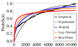
(a) Empirical CDF vs. theoretical CDDs (CCASAT)

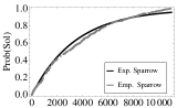
(b) Empirical CDF vs. theoretical CDF (Sparrow)

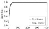
(c) Empirical CDF vs. predicted CDF using 384 cores (Sparrow)

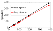
(d) Speedup (Sparrow)

Figure 2: Performance summary on crafted-1

Interestingly, the phase transition point also seems to have important consequences in the parallel performance of local search algorithms. For Sparrow at least, which is the solver with an overall better speedup factor, the instances in the phase transition region are lognormally distributed, while instances outside the phase transition are shifted-exponentially distributed. Another interesting aspect is that in theory the probability of returning a solution in no iterations is non-null because of the (uniform) random initialization. However, in practice a minimum number of steps is in general required to reach a solution cf. [Hoos and Stützle (1999), Ribeiro et al. (2012)] for the sequential case, and therefore experimental data may be better approximated by a shifted distribution with $x_{0}>0$, as it is the case in the random instances. This leads to a non-linear speedup with a finite limit, even in the case of an exponential distribution. Indeed, the experimental speedup for both CCASAT and Sparrow on random instances is far from linear. On the contrary, Sparrow on crafted instances has a linear speedup which could be explained by the fact that the minimal runtime is negligible w.r.t. the mean time (i.e., $1/\lambda$ for an exponential distribution). Therefore, the statistical test succeed for $x_{0}\simeq 0$. This suggests that, in general, the comparison between the minimal time and the mean time is a key element for the study of the parallel behavior.

We do not discard that other parameters for the reference solvers would lead to other theoretical distributions (e.g. exponential distribution for random instances). In [Kroc et al. (2010)] the authors showed that a well-tuned version of WalkSAT is exponentially distributed for instances in the phase transition region. However, we experimented by increasing the ps (smoothing probability) parameter of Sparrow and still obtained the same theoretical distribution. In addition, when ps is too high the solver was unable to solve the instances within the 3 hour time limit. Unfortunately, CCASAT is only available in binary form, and it is not possible to experiment with other parameters for the solver.

We expect this work to have significant implications in the area of automatic parameter tuning to devise scalable local search algorithms. Currently, most parameter tuning tools (e.g. [Hutter et al. (2009), Ansótegui et al. (2009)]) are designed to improve the expected mean (or median) runtime, however as observed in this paper, unless the algorithms exhibit a non-shifted exponential distribution, their parallel performance is far from linear and varies from algorithm to algorithm.

5 Conclusions and Future Work

This paper has presented a model to estimate and evaluate the performance of parallel local search algorithms for SAT. This model, based on order statistics, predicts the parallel runtime execution of a given local search algorithm by analyzing the runtime distribution of its sequential version. Interestingly, we have observed that, for the two different algorithms and the variety of instances considered in this study, the runtime distribution can be characterized using two types of distributions: exponential (shifted and non-shifted) and lognormal.

Extensive experimental results using the best local search solvers from the previous SAT competition, indicate that the model accurately matches the parallel performance of the empirical experiments up to 384 cores. Moreover, the theoretical model confirms the empirical results reported in the literature for local search algorithms [Arbelaez and Codognet (2013), Shylo et al. (2011)] in showing that the best sequential local search solver is not always the best one in parallel settings.

A natural extension of this work would consist in estimating the parallel performance of a given algorithm for unseen instances, even without full sequential execution. To this end, we plan to combine the statistical model presented in this paper with the extensive literature for predicting the runtime a of a given sequential algorithm (see [Xu et al. (2008)]). In addition, we also plan to investigate the application of more (complex) distributions to characterize the distribution of other local search algorithms (e.g. CCASAT for crafted instances).

References

- Aiex et al. (2002) Aiex, R., Resende, M., and Ribeiro, C. 2002. Probability Distribution of Solution Time in GRASP: An Experimental Investigation. Journal of Heuristics 8, 343–373.
- Aiex et al. (2007) Aiex, R., Resende, M., and Ribeiro, C. 2007. TTT Plots: A Perl Program to Create Time-to-Target Plots. Optimization Letters 1, 355–366.
- Ansótegui et al. (2009) Ansótegui, C., Sellmann, M., and Tierney, K. 2009. A Gender-Based Genetic Algorithm for the Automatic Configuration of Algorithms. In 15th International Conference on Principles and Practice of Constraint Programming, I. P. Gent, Ed. LNCS, vol. 5732. Springer, Lisbon, Portugal, 142–157.
- Arbelaez and Codognet (2012) Arbelaez, A. and Codognet, P. 2012. Massivelly Parallel Local Search for SAT. In ICTAI’12. IEEE Computer Society, Athens, Greece, 57–64.
- Arbelaez and Codognet (2013) Arbelaez, A. and Codognet, P. 2013. From Sequential to Parallel Local Search for SAT. In 13th European Conference on Evolutionary Computation in Combinatorial Optimisation (EvoCOP’13). To appear.
- Arbelaez and Hamadi (2011) Arbelaez, A. and Hamadi, Y. 2011. Improving Parallel Local Search for SAT. In Learning and Intelligent Optimization, 5th International Conference, LION’11, C. A. C. Coello, Ed. LNCS, vol. 6683. Springer, 46–60.
- Babai (1979) Babai, L. 1979. Monte-Carlo Algorithms in Graph Isomorphism Testing. Research Report D.M.S. No. 79-10, Université de Montréal.
- Balint and Fröhlich (2010) Balint, A. and Fröhlich, A. 2010. Improving Stochastic Local Search for SAT with a New Probability Distribution. In SAT’10, O. Strichman and S. Szeider, Eds. LNCS, vol. 6175. Springer, Edinburgh, UK, 10–15.
- Cai et al. (2012) Cai, S., Luo, C., and Su, K. 2012. CCASAT: Solver description. In SAT Challenge 2012: Solver and Benchmark Descriptions. Vol. B-2012-2 of Department of Computer Science Series of Publications B. University of Helsinki, 13–14.
- David and Nagaraja (2003) David, H. and Nagaraja, H. 2003. Order Statistics. Wiley series in probability and mathematical statistics. Probability and mathematical statistics. John Wiley.
- Hoos and Stütze (2005) Hoos, H. and Stütze, T. 2005. Stochastic Local Search: Foundations and Applications. Morgan Kaufmann.
- Hoos and Stützle (1998) Hoos, H. H. and Stützle, T. 1998. Evaluating Las Vegas Algorithms: Pitfalls and Remedies. In Proceedings of the Fourteenth Conference on Uncertainty in Artificial Intelligence, UAI’98. Morgan Kaufmann, 238–245.
- Hoos and Stützle (1999) Hoos, H. H. and Stützle, T. 1999. Towards a Characterisation of the Behaviour of Stochastic Local Search Algorithms for SAT. Artif. Intell. 112, 1-2, 213–232.
- Hutter et al. (2009) Hutter, F., Hoos, H. H., Leyton-Brown, K., and Stützle, T. 2009. ParamILS: An Automatic Algorithm Configuration Framework. Journal of Artificial Intelligence Research 36, 267–306.
- Kroc et al. (2010) Kroc, L., Sabharwal, A., and Selman, B. 2010. An Empirical Study of Optimal Noise and Runtime Distributions in Local Search. In SAT’10, O. Strichman and S. Szeider, Eds. LNCS, vol. 6175. Springer, Edinburgh, UK, 346–351.
- Luby et al. (1993) Luby, M., Sinclair, A., and Zuckerman, D. 1993. Optimal speedup of las vegas algorithms. In ISTCS. 128–133.
- Maneva and Sinclair (2008) Maneva, E. and Sinclair, A. 2008. On the Satisfiability Threshold and Clustering of Solutions of Random 3-SAT Formulas. Theoretical Computer Science 407, 1-3, 359–369.
- Martins et al. (2012) Martins, R., Manquinho, V., and Lynce, I. 2012. An Overview of Parallel SAT Solving. Constraints 17, 304–347.
- Munoz et al. (2012) Munoz, P., Barrero, D., and Moreno, M. 2012. Run-Time Analysis of Classical Path-Planning Algorithms. In Proceedings of SGAI 2012, Research and Development in Intelligent Systems XXIX. Springer Verlag, 137–148.
- Nadarajah (2008) Nadarajah, S. 2008. Explicit Expressions for Moments of Order Statistics. Statistics & Probability Letters 78, 2 (Feb.), 196–205.
- Pardalos et al. (1995) Pardalos, P. M., Pitsoulis, L. S., Mavridou, T. D., and Resende, M. G. C. 1995. Parallel Search for Combinatorial Optimization: Genetic Algorithms, Simulated Annealing, Tabu Search and GRASP. In Parallel Algorithms for Irregularly Structured Problems (IRREGULAR). 317–331.
- Pardalos et al. (1996) Pardalos, P. M., Pitsoulis, L. S., and Resende, M. G. C. 1996. A Parallel Grasp for MAX-SAT Problems. In 3rd International Workshop on Applied Parallel Computing, Industrial Computation and Optimization, J. Wasniewski, J. Dongarra, K. Madsen, and D. Olesen, Eds. LNCS. Springer, Lyngby, Denmark.
- Pham and Gretton (2007) Pham, D. N. and Gretton, C. 2007. gNovelty+. In Solver description, SAT competition 2007.
- Ribeiro et al. (2012) Ribeiro, C., Rosseti, I., and Vallejos, R. 2012. Exploiting Run Time Distributions to Compare Sequential and Parallel Stochastic Local Search Algorithms. Journal of Global Optimization 54, 405–429.
- Shylo et al. (2011) Shylo, O. V., Middelkoop, T., and Pardalos, P. M. 2011. Restart strategies in Optimization: Parallel and Serial Cases. Parallel Computing 37, 1, 60–68.
- Truchet et al. (2013) Truchet, C., Richoux, F., and Codognet, P. 2013. Prediction of Parallel Speed-ups for Las Vegas Algorithms. In Proceedings of ICPP-2013, 42nd International Conference on Parallel Processing, J. Dongarra and Y. Robert, Eds. IEEE Press.
- Van Gelder (2011) Van Gelder, A. 2011. Careful Ranking of Multiple Solvers with Timeouts and Ties. In SAT’11, K. Sakallah and L. Simon, Eds. Lecture Notes in Computer Science, vol. 6695. Springer, Ann Arbor, MI, USA, 317–328.
- Verhoeven and Aarts (1995) Verhoeven, M. and Aarts, E. 1995. Parallel Local Search. Journal of Heuristics 1, 1, 43–65.
- Verhoeven (1996) Verhoeven, M. G. A. 1996. Parallel local search. Ph.D. thesis, University of Eindhoven, Eindhoven, Netherlands.
- Wolfram (2003) Wolfram, S. 2003. The Mathematica Book, 5th edition. Wolfram Media.
- Xu et al. (2008) Xu, L., Hutter, F., Hoos, H. H., and Leyton-Brown, K. 2008. Satzilla: Portfolio-based algorithm selection for sat. Journal of Artificial Intelligence Research 32, 565–606.