Verifix: Post-Training Correction to Improve Label Noise Robustness with Verified Samples

Abstract

Label corruption, where training samples have incorrect labels, can significantly degrade the performance of machine learning models. This corruption often arises from non-expert labeling or adversarial attacks. Acquiring large, perfectly labeled datasets is costly, and retraining large models from scratch when a clean dataset becomes available is computationally expensive. To address this challenge, we propose Post-Training Correction, a new paradigm that adjusts model parameters after initial training to mitigate label noise, eliminating the need for retraining. We introduce Verifix, a novel Singular Value Decomposition (SVD) based algorithm that leverages a small, verified dataset to correct the model weights using a single update. Verifix uses SVD to estimate a Clean Activation Space and then projects the model’s weights onto this space to suppress activations corresponding to corrupted data. We demonstrate Verifix’s effectiveness on both synthetic and real-world label noise. Experiments on the CIFAR dataset with $25\%$ synthetic corruption show $7.36\%$ generalization improvements on average. Additionally, we observe generalization improvements of up to $2.63\%$ on naturally corrupted datasets like WebVision1.0 and Clothing1M. Find our code at https://github.com/sangamesh-kodge/Verifix.git.

1 Introduction

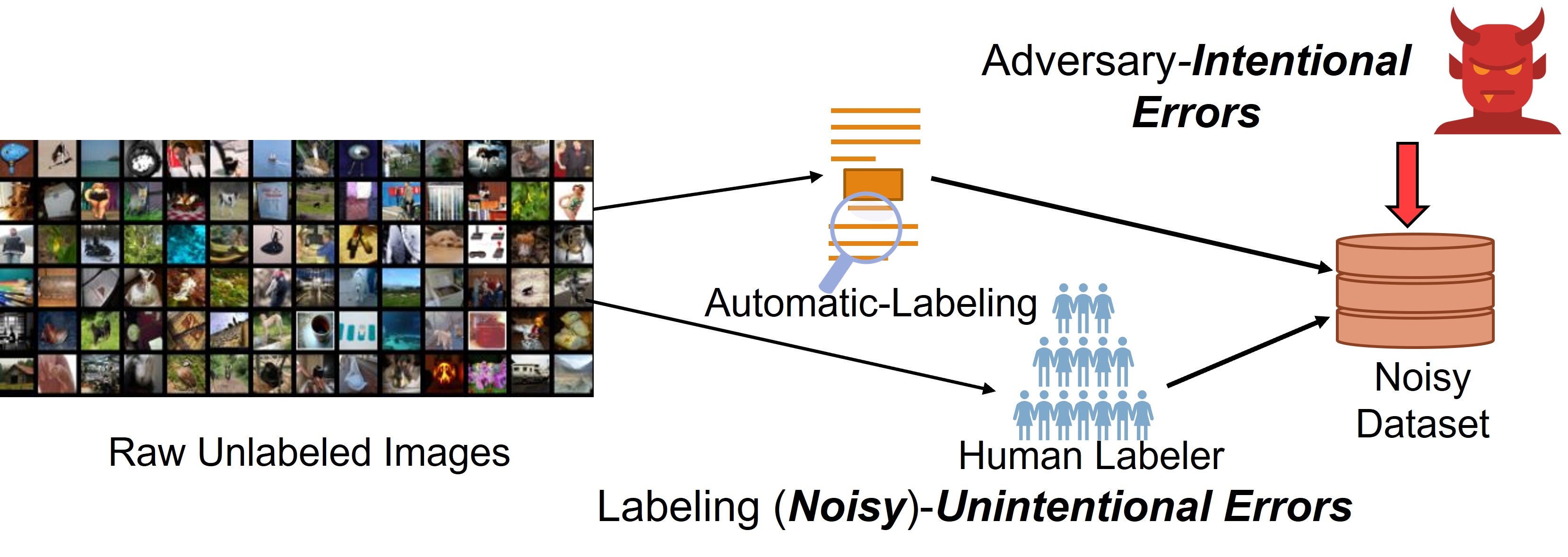
(a) Errors in Dataset Creation.

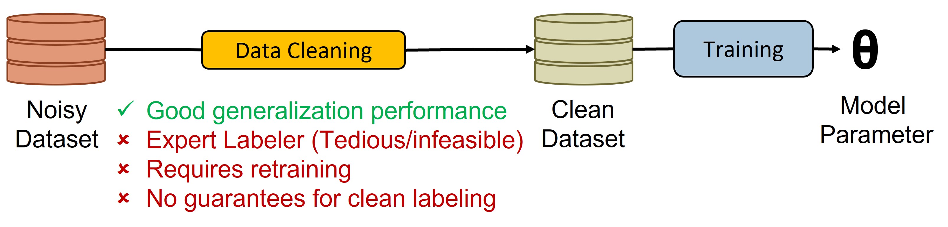
(b) Domain 1 - Dataset cleaning

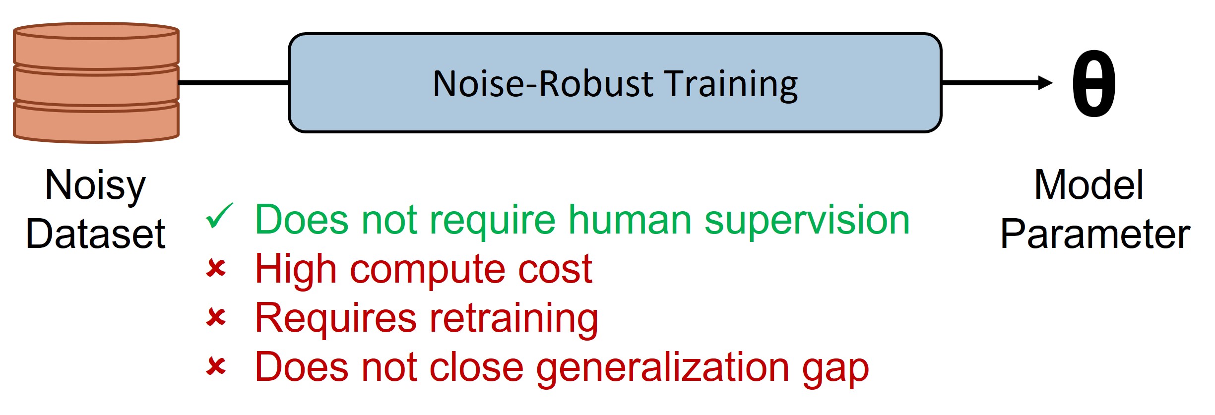
(c) Domain 2 - Noise-Robust Training

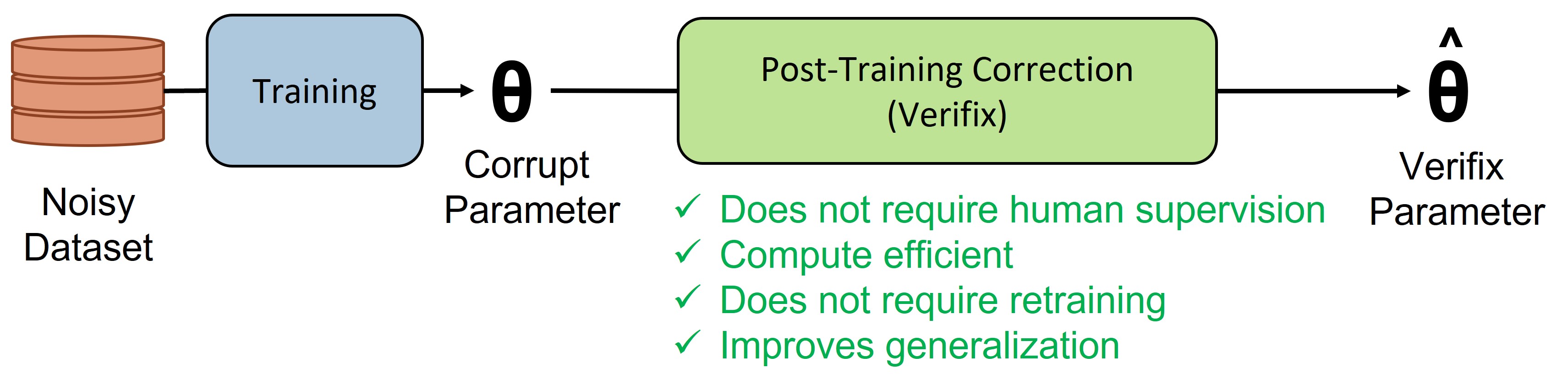
(d) Proposed - Post-Training Correction

Figure 1: Overview of Label Noise Handling Components. (a) Illustrates the various sources of label noise - Intentional and Unintentional Errors, (b) Explores Data Cleaning approaches [30, 29, 10], (c) Presents Noise-Robust Training methods [9, 47], and (d) shows the proposed Post-Training Correction paradigm.

Deep learning has consistently showcased cutting-edge performance across a spectrum of learning tasks, spanning domains such as natural language processing and computer vision. These achievements largely stem from the substantial increase in available data, enabling more effective model training. However, the sheer size of these datasets poses challenges in ensuring accurate labeling. Recent studies such as [31], have revealed the prevalence of labeling errors in widely used benchmark datasets. These labeling errors can originate from various sources and fall into two broad categories: intentional and unintentional errors (Figure 1(a)). Intentional errors, often associated with data poisoning attacks[36], include label-flipping attacks where an adversary maliciously corrupts the training labels. These attacks aim to (1) compromise the model’s performance [1, 16], affecting the usability of the model for the desired application; (2) gain unauthorized access to circumvent the system of a safety-critical application through a backdoor attack [4]; or (3) render models more susceptible to membership inference attacks [5], unethically obtaining access to training data. Another source of label errors, called Unintentional errors, arises from the labeling process itself. For instance, crowd-sourcing and auto-labeling are inherently error-prone [35], and errors persist even when efforts are made to control them [22, 48]. While deep learning models exhibit robustness to a certain degree of label noise [33, 12], they are not immune to label noise, as demonstrated in [39].

To enhance label noise robustness, researchers have primarily concentrated on two research domains. Domain 1 (Figure 1(b)), focuses on dataset cleaning to ensure trustworthy model training by identifying and correcting mislabeled samples before learning. The naive approach of manual re-labeling by experts is infeasible for large datasets and also shown to be error-prone [35]. Hence, the majority of works focus on automated detection of corrupt samples [30, 29, 10]. However, many automated label corruption detection approaches leverage learning dynamics, incurring significant computational overhead. Domain 2 (Figure 1(c)) focuses on developing noise-robust algorithms to tackle label noise, this includes Sharpness-Aware Minimization (SAM)[9], MixUp[47], MentorMix[17], and dropout regularization [19]. Some of these approaches use compute-intensive training pipelines to counter the effect of label corruption in the training data. Despite these efforts, both domains have limitations: they can be computationally expensive, may not fully eliminate performance gaps compared to clean data training, and often necessitate complete retraining if label noise is discovered later. This presents a significant obstacle for large models trained on large datasets. To address the aforementioned challenges, we introduce a novel domain depicted in Figure 1(d)—Post-Training Correction. This proposed domain focuses on adjusting model parameters after the training process, thereby eliminating the computational expense associated with full retraining.

In this work, we present Verifix, a novel Post-Training Correction algorithm that compensates for the effects of label noise using a small subset of verified clean training samples. Below, we outline the three essential components of Verifix (as depicted in Figure 2):

• Trusted Data Estimation (Section 4.2) - Verifix leverages input curvature scores [10, 32] to automatically identify a subset of correctly labeled samples, $\mathcal{D}_{Trust}$, from a pre-trained model. Our emphasis on low-curvature samples yields up to a $1.06\%$ improvement in generalization scores compared to random sampling from clean training data.

• Activation Alignment (Section 4.3) - Verifix performs Singular Value Decomposition (SVD) on the trusted dataset, $\mathcal{D}_{Trust}$, to decompose it into principal components. The left singular matrix ($U$) forms the basis directions of activation patterns associated with clean (trusted) data. We obtain the scaled basis vectors, where the basis directions $U$ are scaled according to the explained variance using the importance scaling $\Lambda$. This gives us the Activation Alignment Matrix.

• Weight Update (Section 4.1) - Verifix leverages the Activation Alignment Space to update model weights, selectively reducing the influence of activations likely associated with corrupted data.

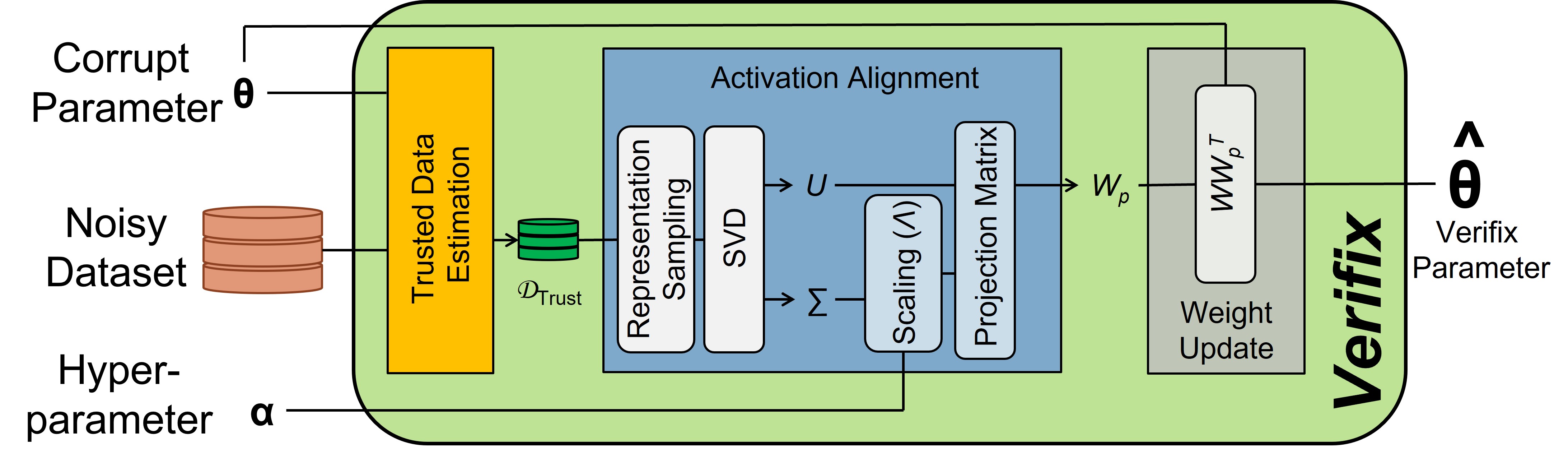
Figure 2: Overview of the proposed Verifix algorithm. Here, $\theta$ denotes the model weights which comprises of the layer weights represented by $W$.

We demonstrate the effectiveness of Verifix on both synthetically corrupted and real-world datasets. First, we present results for synthetically corrupted data by manually introducing noise into the CIFAR10/100 dataset [23]. When evaluating Verifix on ResNet18 [15] and VGG11 [37] network architectures, we observe significant improvement in generalization of $7.36\%$ under $25\%$ label corruption. Additionally, we test our algorithm on the Mini-WebVision [17], WebVision1.0[25], and Clothing1M [46] datasets, which contain naturally occurring noisy labels. On these real-world datasets, Verifix achieves up to $2.63\%$ generalization improvement on average despite the presence of natural label noise.

In summary, the contributions of this paper are:

1. We propose Post-Training Correction (Figure 1(d)), a label noise correction paradigm designed to improve model generalization. This paradigm focuses compute efficient post-training model parameter adjustments avoiding model retraining.

2. We propose Verifix, a Singular Value Decomposition (SVD) based technique, which establishes a new baseline to improve the generalization performance of the model trained with noisy labels Post-Training. Verifix automates the selection of trusted samples using curvature scores and updates model weights in a single step, offering significant computational savings over standard retraining approaches.

3. We empirically validate the performance of our method for both synthetically and naturally corrupted datasets, and show a generalization improvement up to $10.19\%$ (for $25\%$ corruption) and $2.63\%$, respectively.

2 Related Work

We survey existing works in two key domains of label noise research:

2.0.1 Data Cleaning (Domain 1) :

This direction of research focuses on detecting and correcting or removing mislabeled samples within the training dataset, ensuring the model only learns from accurately labeled data. The naive human (expert) in the loop relabeling is tedious and often error-prone [35]. In response, the research in this domain primarily focuses on the automatic detection of mislabeled samples. Several works [8, 2, 41, 14, 38, 50, 20] train an ensemble of models to filter out the incorrectly labeled samples. A major limitation of these ensemble-based approaches is their computational expense, especially for large datasets where training multiple models can be infeasible. To address this challenge, several studies have focused on leveraging training dynamics to identify label noise, including methods such as using cross-validation on noisy splits [3], learning time [26, 45], forgetting time [29], train-set confidence [30] or thorough input loss curvature [10, 32]. While these approaches reduce computational overheads compared to ensemble-based methods, a remaining challenge lies in distinguishing between truly difficult examples and those that are mislabeled [10]. Additionally, approaches in this domain still necessitate retraining models on the filtered dataset, failing to fully leverage the models learned on the initial noisy data. In contrast, our proposed Post-Training Correction paradigm seeks computationally efficient ways to directly adjust the corrupted model. This approach is crucial for large datasets and models where retraining might be computationally intractable.

2.0.2 Noise-Robust Training (Domain 2) :

This domain of algorithms tackles the challenge of label noise through the development of training techniques and loss functions that are inherently less sensitive to mislabeled data. Regularization techniques, such as dropout [19] (which introduces randomness during training) and label smoothing [28, 44] (which softens target labels), help prevent overfitting and improve label noise robustness. Robust loss functions like symmetric cross-entropy [43] and Mean Absolute Error (MAE) reduce the impact of noisy labels compared to standard cross-entropy loss. Optimization methods like Sharpness-Aware Minimization (SAM) [9] promote flatter loss landscapes, which are associated with better generalization under label noise. Additionally, curriculum and self-paced learning [18, 49] gradually increase the difficulty of training examples, helping the model learn robust features before encountering noise. Data augmentation and mixup techniques (e.g., MixUp [47], DivideMix [24], MentorMix[17]) smooth training distributions, encouraging less abrupt decision boundaries and further enhancing robustness. While these robust algorithms offer improvement over standard training, they still have limitations. Some can be computationally expensive to implement or may reduce performance on clean datasets. Additionally, they often underperform compared to models trained with perfectly labeled data. Our proposed algorithm is orthogonal to these techniques and can be used in combination to further close this generalization gap.

3 Background

3.1 Singular Value Decomposition

A rectangular matrix $A$ in $\mathbb{R}^{d\times n}$ can be decomposed with Singular Value Decomposition (SVD) [7] as

$$A=U\Sigma V^{T}.$$ (1)

Here, $U\in\mathbb{R}^{d\times d}$ and $V\in\mathbb{R}^{n\times n}$ are orthogonal matrices and are called left singular matrix and right singular matrix, respectively. $\Sigma\in\mathbb{R}^{d\times n}$ is a diagonal matrix comprising singular values. Each column vector of $U$ is $d$-dimensional and these vectors form the basis of the column space of $A$. The amount of variance explained by the $i^{th}$ vector of $U$, $u_{i}$, having singular value of $\sigma_{i}$ is proportional to $\sigma_{i}^{2}$ and hence the fraction variance explained is given by

$$\widetilde{\sigma}_{i}=\sigma_{i}^{2}/(\sum_{j=1}^{d}(\sigma_{j}^{2})).$$ (2)

3.2 Problem Formulation

Let the training dataset be defined as $\mathcal{D}_{Tr}=\{(x_{i},y_{i})\}_{i=1}^{N_{Tr}}$, where $N_{Tr}$ represents the total number of training samples. Here, $x_{i}$ denotes the input features with the corresponding label $y_{i}$. The validation dataset is represented as $\mathcal{D}_{Val}=\{(x_{i},y_{i})\}_{i=1}^{N_{Val}}$, and the test dataset is denoted as $\mathcal{D}_{Te}=\{(x_{i},y_{i})\}_{i=1}^{N_{Te}}$, where $N_{Val}$ and $N_{Te}$ signify the number of validation samples and test samples, respectively. Consider a deep neural network that approximates the mapping from input data $x_{i}$ to the corresponding label $y_{i}$ through the function $y=f(\theta,x_{i})$, where $\theta$ denotes the network’s weights or parameters. These parameters are trained through gradient descent-based optimization on the samples from the training dataset $\mathcal{D}_{Tr}$, and the validation dataset $\mathcal{D}_{Val}$ is used for tuning the hyperparameters. For a network with strong generalization performance, we expect that the relationship $y_{i}=f(\theta,x_{i})$ holds true for a substantial number of samples $(x_{i},y_{i})\in\mathcal{D}_{Te}$. Since network parameters are trained to minimize the empirical risk or loss $\mathcal{L}(y_{i},f(\theta,x_{i}))$ on the samples from $\mathcal{D}_{Tr}$, the presence of label corruption or noise in a portion of the training dataset can hamper network’s generalization ability thus decreasing the performance.

$$\begin{split}\text{Given : }&\theta_{*}=\text{{train}}(\mathcal{D}_{Tr})\\ \text{Obtain : }&\hat{\theta}_{*}=\text{{post\_training\_correction}}(\theta_{*},\mathcal{D}_{Tr})\\ \text{ s.t. }&y_{i}\approx f(\hat{\theta}_{*},x_{i})\approx f(\theta_{*}^{cln},x_{i})\\ \text{ where }&(x_{i},y_{i})\in\mathcal{D}_{Val}\text{ and }\theta_{*}^{cln}=\text{{train}}(\mathcal{D}_{Tr}^{cln})\end{split}$$ (3)

The objective of a label noise correction algorithm is to enhance the generalization performance of a network trained on data, $\mathcal{D}_{Tr}$ containing noisy/corrupted labels. This essentially involves removing the influence of corrupted samples from the network parameters $\theta_{*}$ trained on corrupted data. Such an algorithm is expected to produce parameters $\hat{\theta}_{*}$ that closely matches the functionality of the model with parameters $\theta_{*}^{cln}$, which were trained on $\mathcal{D}_{Tr}^{cln}\subset\mathcal{D}_{Tr}$, a subset comprising correctly labeled samples. This objective be formally expressed as Equation 3.

4 Verifix

A network trained on a dataset $\mathcal{D}_{Tr}$ with corrupted labels is prone to overfit on the incorrect samples within the training data. Such a network is likely to produce spurious intermediate activations to incorporate the incorrect sample-label mapping. Our label correction approach (Figure 2), outlined in Algorithm 1, aims to align these intermediate activations with representative or trusted activations. In the next Subsection, we explain our weight update mechanism which enables us to modify the model weights to remove the influence of corrupt data.

4.1 Weight Update

Consider a linear layer with parameters $W$ that generates the output activation $a_{out}$, given by $a_{out}=a_{in}W^{T}$. We align the input activations of this layer with the trusted activations by projecting the activations $a_{in}$ onto a strategically constructed projection matrix $W_{p}$, also known as the Activation Alignment matrix. This projection would suppress the noisy activation as shown in Figure 3(c). This results in updating the output activation as $\widehat{a}_{out}=(a_{in}W_{p})W^{T}$. We rewrite this equation to absorb the alignment matrix $W_{p}$ into the layer weights, effectively updating the weights as $\widehat{W}=WW_{p}^{T}$, as detailed in Equation 4. This weight update rule explains the update_parameter procedure in line 7 of Algorithm 1. In the rest of this Section, our focus is on obtaining the alignment matrix $W_{p}$.

$$\widehat{a}_{out}=\underbrace{(a_{in}W_{p})}_{\text{Activation Projection}}W^{T}=a_{in}(\underbrace{WW_{p}^{T}}_{\text{Weight Update}})^{T}=a_{in}\widehat{W}^{T}$$ (4)

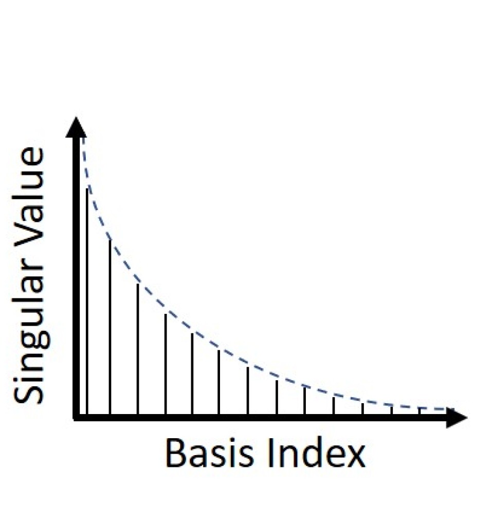
(a) Singular Values

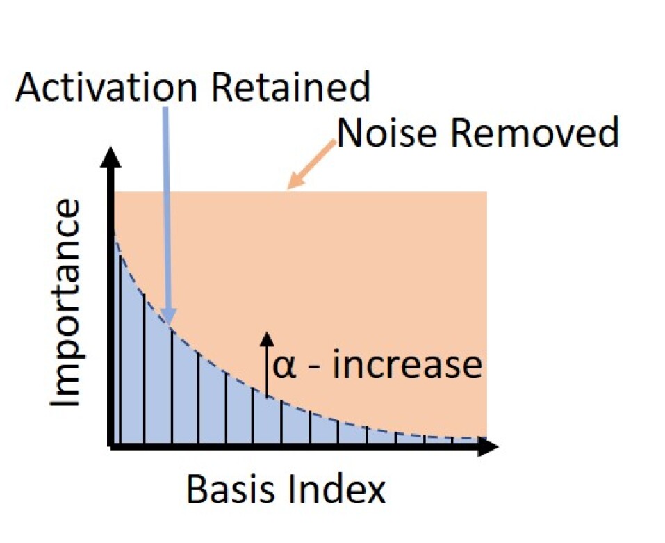
(b) Importance Scaling

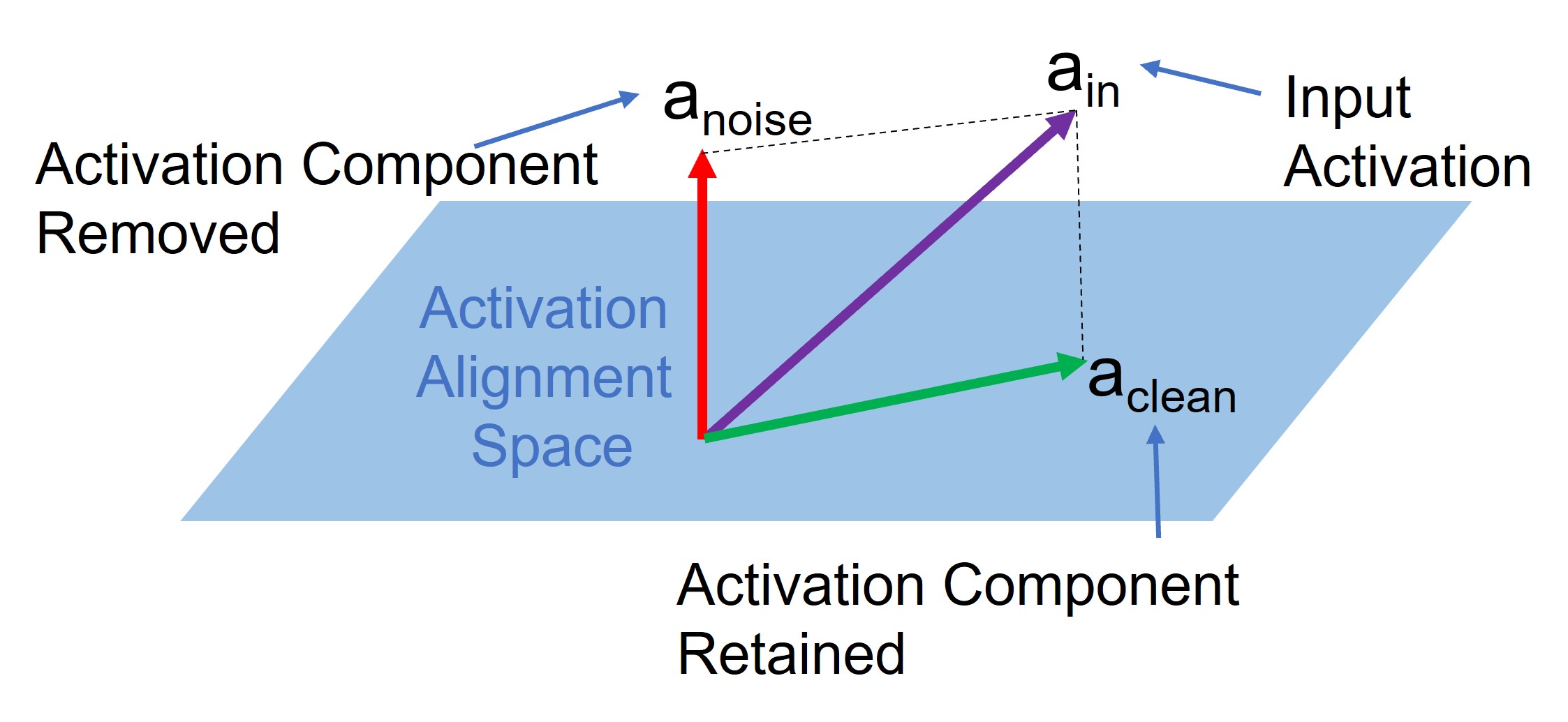
(c) Activation Alignment

Figure 3: (a) Singular value distribution obtained through SVD on the Representative activations. (b) Effect of $\alpha$ in importance scaling Equation 8 and (c) the projection of noisy activation on Activation Alignment Space to obtain clean activations.

Input: $\theta_{*}$ is the parameters of the original model; $\mathcal{D}_{Tr}$ is the training dataset with corrupt labels, and $\alpha$ is a hyperparameter called scaling coefficient.

procedure post_training_correction( $\theta_{*}$, $\mathcal{D}_{Tr}$, $\alpha$)
1. $\mathcal{D}_{Trust}$ = get_trusted($\theta_{*}$, $\mathcal{D}_{Tr}$) // Section 4.2
2. $R$ = representation($\theta_{*}$, $\mathcal{D}_{Trust}$) // Eqn. 6, 7
3. for each layer with parameter $W^{l}_{*}$ $\in\theta_{*}$ do
4.     $U^{l}$, $\Sigma^{l}$ = SVD($R^{l}$) // Eqn. 1
5.     $\Lambda^{l}$ = scale_importance($\Sigma^{l}$, $\alpha$ ) // Eqn. 8
6.     $W_{p}^{l}$ = $U^{l}\Lambda^{l}(U^{l})^{T}$ // Eqn. 9
7.     $\widehat{W}^{l}_{*}=$ update_parameter($W_{p}^{l}$, $W^{l}_{*}$ ) // Eqn. 4
8. return $\hat{\theta}_{*}$ // where $\hat{\theta}_{*}$ is updated parameters

Algorithm 1 Verifix algorithm.

Obtaining a high-quality alignment matrix requires access to representative activations for ‘trusted’ samples or the samples in $\mathcal{D}_{Tr}$ with correct labels. We, therefore, divide the step of obtaining $W_{p}$ into two parts: (1) estimating a few correctly labeled or ‘trusted’ samples from $\mathcal{D}_{Tr}$, as presented in Section 4.2, and (2) obtaining the Activation Alignment Matrix using these samples outlined in Section 4.3.

4.2 Trusted Data Estimation

We define the trusted dataset, $\mathcal{D}_{Trust}=\{(x_{i},y_{i})\}_{i=1}^{N_{Trust}}$, as a subset of $\mathcal{D}_{Tr}$ containing a few ($N_{Trust}$) correctly labeled samples. This can be obtained by employing human expert labelers. Instead, in this paper we propose an automatic approach using the curvature scores [11, 10] of the training samples to identify samples that are correctly labeled. Note we use the curvature at the last epoch rather than the average curvature over all the training epochs [32]. This score is given by Equation 5

$$Curv(x_{i},y_{i})=\frac{1}{n}\sum_{j=0}^{n}\left\lVert\frac{\partial(L(x_{i}+hv_{j},y_{i})-L(x_{i},y_{i}))}{\partial x_{i}}\right\rVert_{2}^{2}$$ (5)

Where $n$ is the number of Rademacher variables $v_{j}$ to average over. Using low curvature input samples is a good way to obtain trusted data. It was shown in [10, 11] that curvature performs well when compared to other mislabeling detection methods since it captures network memorization [32]. We compute curvature scores for all the samples in $\mathcal{D}_{Tr}$ and select the $N_{Trust}$ samples with the lowest curvature scores to obtain the trusted datasets $\mathcal{D}_{Trust}$. These samples are used to obtain the Activation Alignment Matrix in the next Subsection.

4.3 Activation Alignment

To estimate the activation basis for the clean samples, we gather the input activations of linear and convolutional layers, as detailed below.

4.3.1 Representation Sampling :

For the $l^{th}$ linear or convolutional layer of the network, we collect the input activation $a_{in}$ and store these activation in a representation matrix $R^{l}$. This matrix captures representative information from the trusted samples in the input activations. It is utilized to estimate the trusted activation basis. Next, we elaborate on the details of this representation matrix [34] for each type of layer.

1. Linear Layer - For a linear layer, the representation matrix, as given by Equation 6, stores the input activations for all the samples in $\mathcal{D}_{Trust}$.

   $$R_{linear}=[(a_{in}^{i})_{i=1}^{N_{Trust}}]$$ (6)

   Here, $a_{in}$ is the input activation for the linear layer.

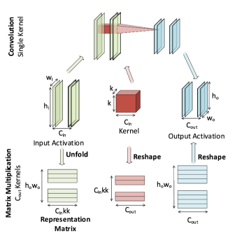
Figure 9: Representing convolution as matrix multiplication to enable weight update for unlearning. Each convolution kernel operates on patches of size $C_{in}\times k\times k$ in a sliding window fashion to produce an output map of size $h_{o}\times w_{o}$. The total number of patches is hence $n_{p}=h_{o}w_{o}$ for each pixel in the output activation map. The Unfold operation reshapes all these input patches for each sliding window to give a matrix of size $h_{o}w_{o}\times C_{in}kk$. Unfolding the input activation and reshaping the weight kernel mathematically converts convolution into matrix multiplication operation as shown in the figure. The Unfolded input activations are collected as Representation Matrix for estimating Spaces using SVD.

2. Convolutional Layer - For the convolutional layer, we express the convolution operation as matrix multiplication to apply the weight update rule proposed in Equation 4. This is achieved through the unfold [27] operation where the convolution operation is represented as matrix multiplication. Let the kernel size of the convolutional layer be $C_{out}\times C_{in}\times k\times k$, where $C_{in}$ represents the number of input channels, $C_{out}$ denotes the number of output channels and $k$ is the kernel size. The unfold operation would flatten all the patches in the input activations on which this kernel operates in a sliding window fashion, which gives us a matrix of size $n_{p}\times C_{in}kk$. Here, $n_{p}$ represents the number of patches in the activation $a_{in}^{i}$ of the $i^{th}$ sample in $\mathcal{D}_{Trust}$. This process allows us to represent convolution as matrix multiplication between the reshaped weights of size $C_{out}\times{C_{in}kk}$ and the unfolded activation of $a^{i}_{in}$ of size $n_{p}\times{C_{in}kk}$. Figure 9 in Appendix details the conversion of the convolution operation into the matrix multiplication operation. The unfolded activations of all the samples are concatenated and stored in the representation matrix as represented by Equation 7. We use the reshaped convolutions parameters to update the parameters as given in Equation 4.

   $$R_{conv}=[(\texttt{unfold}(a_{in}^{i})^{T})_{i=1}^{N_{Trust}}]$$ (7)

   The representation procedure in line 2 of Algorithm 1 obtains a list of these representation matrices $R$. The $l^{th}$ element of this list, $R^{l}$, is the representation matrix of the $l^{th}$ linear or convolutional layer of the network.

4.3.2 SVD on Representations :

We perform Singular Value Decomposition (SVD), as given in Equation 1, on the representation matrices $R^{l}$ for the $l^{th}$ layer, as shown in line 4 of Algorithm 1. The SVD procedure provides us with the basis vectors $U$ and the singular values $\Sigma$ for the trusted samples. The $j^{th}$ vector in $U$, $u_{j}$, is a vector having a unit norm and does not capture the importance of this vector. We scale these vectors in proportion to the variance explained by these vectors.

4.3.3 Importance Scaling :

We formulate a diagonal importance matrix $\Lambda$ with the $j^{th}$ diagonal component $\lambda_{j}$ given by Equation 8 [21]. Here, $\widetilde{\sigma}_{j}$ represents the normalized $j^{th}$ singular value, as defined in Equation 2. The effect of such scaling on singular values is shown in Figure 3. The parameter $\alpha\in(0,\infty)$, known as the scaling coefficient, serves as a hyperparameter controlling the scaling of the basis vectors. When $\alpha$ is set to 1, the basis vectors are scaled by the amount of variance they explain. Figure 3(b) shows the effect of changing $\alpha$ on the scaling of the basis vectors. As $\alpha$ increases, the importance score for each basis vector increases and approaches 1 as $\alpha\to\infty$. Conversely, a decrease in $\alpha$ diminishes the importance of the basis vectors, approaching 0 as $\alpha\to 0$. The scale_parameter procedure in line 5 of Algorithm 1 corresponds to this importance-based scaling.

$$\lambda_{i}=\frac{\alpha\widetilde{\sigma}_{i}}{(\alpha-1)\widetilde{\sigma}_{i}+1}$$ (8)

4.3.4 Projection Matrix :

The Activation Alignment Matrix $W_{p}$ is obtained in line 6 of Algorithm 1 using the basis vectors $U$ and the scaled importance matrix $\Lambda$ by Equation 9. This matrix projects the input activation into the activations spanned by the trusted samples effectively removing the noise due to the corrupted labels from the training dataset.

$$W_{p}=U\Lambda(U)^{T}$$ (9)

5 Experiments

5.1 Toy Illustration

(a) Clean Dataset.

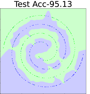
(b) Corrupt Dataset

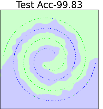
(c) Verifix applied to (b).

Figure 4: Decision boundaries for a network trained the 2D spiral data (a) with full Clean data, (b) with $10\%$ corrupt data and (c) label correction algorithm applied to network trained on corrupt data.

In order to demonstrate our algorithm, we trained a network for binary classification task on clean training data and data where $10\%$ labels were flipped (corrupted) from 2D spiral dataset [42]. Figure 4(a) and 4(b) show the decision boundary of the model for the former and later cases respectively. We observe that, with label corruption, the test accuracy of the model drops by $4.8\%$ from the model trained without any label corruption. The model trained on noisy data(Figure 4(b)) has a more complex and rough decision boundary which indicates memorization of the corrupt data points leading to a loss in generalization. When Verifix is applied to the model trained on corrupt data (Figure 4(c)), we observe the decision boundary smoothness and we recover the generalization performance.

5.2 Synthetic Noise

We evaluate our algorithm on the CIFAR[23] dataset with synthetic noise, using modified ResNet18 [15] and VGG11 (with BatchNorm) [37] architectures. We introduce random label corruption to $x\%$ of the training data $\mathcal{D}_{Tr}$, creating a corrupted dataset $\mathcal{D}^{cpt}_{Tr}$. This corrupted dataset is further split into Validation ($10\%$) and Training ($90\%$) sets. A subset of the corrupt dataset with correctly labeled samples is called a clean subset of the corrupt dataset and is denoted by $\mathcal{D}^{cln}_{Tr}$. We use the Validation set to tune the hyperparameter $\alpha$ and report test accuracy results in Table 1. Training details are provided in Appendix 0.B.

5.2.1 Benchmarks :

We compare the following models in Table 1: (1) Ideal - Model trained with Stochastic Gradient Descent (SGD) on $\mathcal{D}_{Tr}$, entire dataset with clean labels; (2) Retrain - Model trained with SGD on $\mathcal{D}^{cln}_{Tr}$, clean partition of corrupt dataset; (3) Vanilla - Model trained with SGD on $\mathcal{D}^{cpt}_{Tr}$, entire corrupt dataset; (4)SAM - Model trained with Sharpness-Aware Minimization (SAM) [9] on $\mathcal{D}^{cpt}_{Tr}$; (5)Finetune - Vanilla model further finetuned on a small, randomly selected clean subset of $\mathcal{D}^{cln}_{Tr}$; (6) Verifix_Vanilla - Our method applied to the (pre-trained) Vanilla model; and (7) Verifix_SAM - Our method applied to the SAM model.

5.2.2 Results :

Our results in Table 1 show the Retrain models perform closely match the Ideal model, indicating that mildly reducing dataset size has minimal impact on model generalization [13]. In contrast, the Vanilla model experiences a significant drop in test accuracy, especially at higher noise levels. We observe a $15-20\%$ drop with $25\%$ corruption level for both CIFAR10 and CIFAR100. This highlights the severe impact of label noise on performance. Finetuning the Vanilla model on a small set of trusted samples (1000 for 50 epochs) consistently improves performance. Notably, finetuning on just 1000 samples can boost performance by approximately $8\%$ for a VGG11 model trained on CIFAR10 with $25\%$ corruption (see Finetune in Table 1). Applying our method to the Vanilla model (Verifix_Vanilla) leads to significant improvements on both CIFAR10 and CIFAR100 datasets. With a $25\%$ corruption rate, we observe gains of $11.19\%$ (VGG11) and $6.97\%$ (ResNet18) on CIFAR10, and $7.78\%$ (VGG11) and $3.5\%$ (ResNet18) on CIFAR100.

Table 1: Test Accuracy for label noise removal on CIFAR10 and CIFAR100 datasets trained on VGG11 and ResNet18 architectures with $10\%$ and $25\%$ label corruption. We report the mean and standard deviation across three randomly chosen seeds. Verifix and Finetune methods use 1000 trusted samples. See Appendix 0.C for a lower level of synthetic noise.

	Method	VGG11_BN		ResNet18
		Percentage Mislabeled Samples		Percentage Mislabeled Samples
		10%	25%	10%	25%
CIFAR10	Ideal	$91.18\pm 0.17$		$94.23\pm 0.06$
	Retrain	$90.73\pm 0.15$	$89.60\pm 0.21$	$93.77\pm 0.25$	$93.08\pm 0.21$
	Vanilla	$85.01\pm 0.38$	$72.19\pm 0.33$	$88.66\pm 0.38$	$78.37\pm 0.18$
	SAM	$\textbf{89.96}\pm\textbf{0.1}$	$87.05\pm 0.28$	$90.80\pm 0.13$	$83.76\pm 0.11$
	Finetune	$87.03\pm 0.42$	$81.82\pm 0.25$	$89.49\pm 0.2$	$82.82\pm 0.70$
	VerfixVanilla	$87.78\pm 0.18$	$83.38\pm 0.47$	$90.46\pm 0.10$	$86.96\pm 0.14$
	VerfixSAM	$89.95\pm 0.11$	$\textbf{87.17}\pm\textbf{0.38}$	$\textbf{91.42}\pm\textbf{0.14}$	$\textbf{87.74}\pm\textbf{0.38}$
CIFAR100	Ideal	$67.44\pm 0.18$		$75.34\pm 0.06$
	Retrain	$65.99\pm 0.43$	$63.73\pm 0.52$	$73.89\pm 0.16$	$72.13\pm 0.36$
	Vanilla	$60.66\pm 0.23$	$49.03\pm 0.69$	$68.16\pm 0.40$	$57.60\pm 0.17$
	SAM	$62.58\pm 0.52$	$54.31\pm 0.21$	$69.64\pm 0.18$	$58.82\pm 0.76$
	Finetune	$60.68\pm 0.23$	$49.01\pm 0.70$	$68.42\pm 0.53$	$58.67\pm 0.17$
	VerfixVanilla	$63.10\pm 0.40$	$56.81\pm 0.37$	$69.16\pm 0.16$	$61.42\pm 0.46$
	VerfixSAM	$\textbf{63.80}\pm\textbf{0.50}$	$\textbf{58.33}\pm\textbf{0.11}$	$\textbf{70.21}\pm\textbf{0.16}$	$\textbf{62.19}\pm\textbf{0.66}$

We compare our approach to SAM [9], which is a training technique more robust to label noise but requires double the resources of standard SGD. While SAM s more robust to label noise over the Vanilla model, our method applied to the Vanilla model (Verifix_Vanilla in Table 3) outperforms SAM in most cases with $25\%$ corruption and remains competitive at $10\%$ corruption. The only exception is VGG11 on CIFAR10, where SAM shows slightly higher gains ($2.18\%$ at $10\%$ corruption, $3.67\%$ at $25\%$). Importantly, Verfix_Vanilla demonstrates an average improvement of $0.58\%$ over SAM, highlighting its effectiveness while requiring significantly fewer computational resources. Additionally, applying our method to SAM-trained models (Verifix_SAM in Table 1) further boosts accuracy up to $4.02\%$, achieving the best results in Table 1. This highlights that our method is complementary to existing noise-robust training techniques, offering additional generalization improvements.

Figure 5: Effect of sampling strategy on CIFAR100 dataset for model trained with $25\%$ corrupt labels.

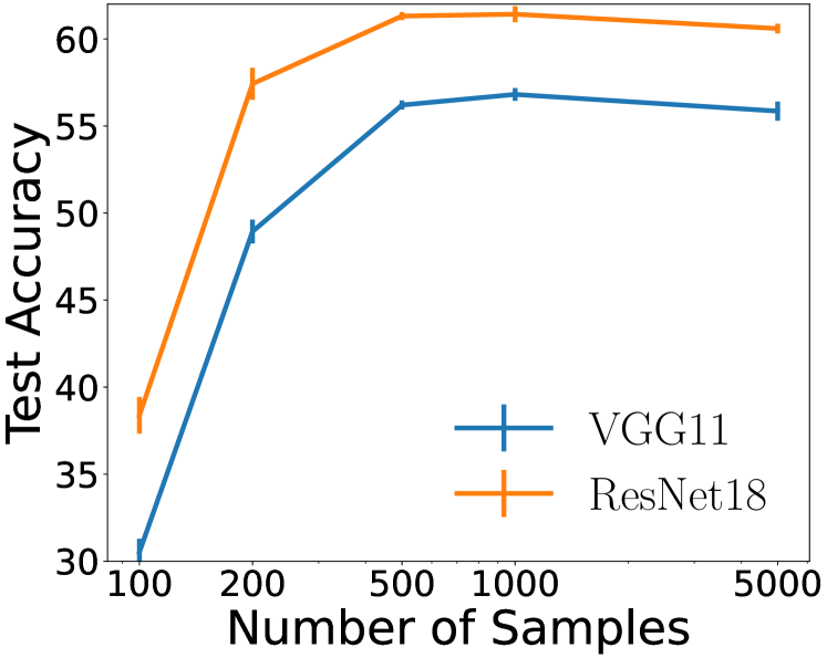
Figure 6: Effect of trusted sample size on CIFAR100 dataset for model trained with $25\%$ corrupt labels.

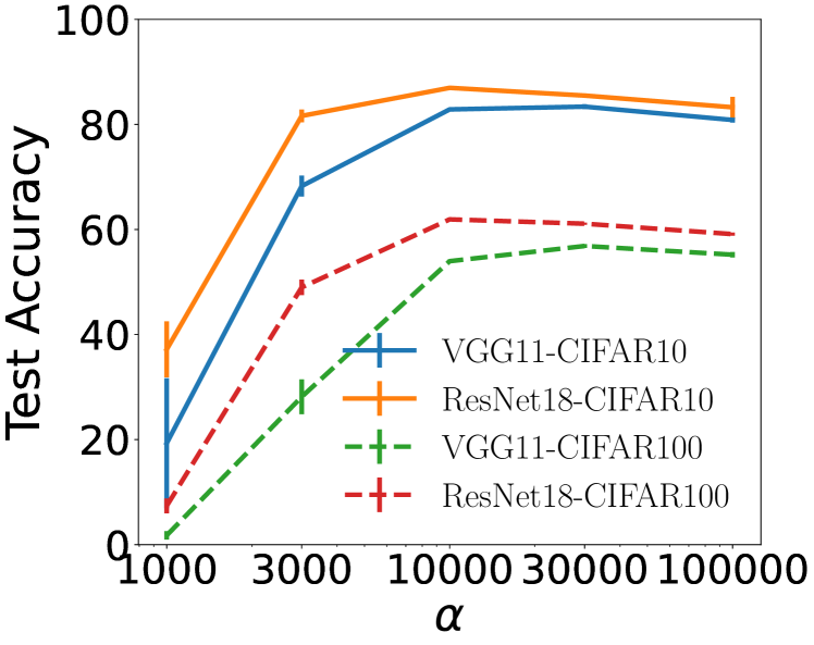
Figure 7: Effect of $\alpha$ for model trained with $25\%$ corrupt labels.

5.3 Analyses

5.3.1 Selecting samples with low curvature improves generalization :

Our approach uses a few trusted samples from the clean portion of the training dataset ($\mathcal{D}^{cln}_{Tr}$). We explored six different sampling strategies in Figure 7. The Expert strategy provides 1000 correctly labeled samples from $\mathcal{D}^{cln}_{Tr}$, requiring access to ground-truth labels. Alternatively, we use curvature scores (Equation 5) to identify likely clean samples from the corrupted dataset $\mathcal{D}^{cpt}_{Tr}$. We sort samples by ascending curvature and select 1000 based on percentile scores (0%, 10%, 25%, 50% strategy) or random sampling from the lower 50% percentile samples (Uniform strategy). By x% sampling strategy, we mean selecting 1000 images after the $x^{th}$ percentile of low-curvature samples. Interestingly, selecting the 1000 lowest curvature samples (0% sampling) consistently outperforms other strategies, suggesting these samples are most beneficial for our method. For CIFAR100 dataset with 0% sampling, we achieve $56.85\%$ and $61.1\%$ test accuracy on VGG11 and ResNet18 model, respectively. We observe that performance decreases as we sample from higher curvature percentiles, with steeper declines for VGG11. Our experiments show an curvature based sampling improves the generalization up to $1.06\%$ for 0% strategy when compared to Expert. Additionally, the Expert sampling strategy gives similar performance to Unifrom strategy ($\sim 55.8\%$ for VGG11 and $\sim 60.55\%$ for ResNet18 on CIFAR100).

5.3.2 Increasing Trusted Sample Size yields diminishing returns in performance :

We study how the number of trusted samples impacts our method’s performance and computational cost. Since representation calculations and SVD are performed on the trusted set, the sample size directly affects compute requirements. Figure 7 shows how test accuracy varies with the number of trusted samples. We observe that increasing the sample size improves accuracy up to 1000 samples, after which there are no significant gains. Therefore, we use 1000 samples in our experiments to balance performance and computational efficiency.

5.3.3 Finding the optimal scaling hyperparameter ($\alpha$) is key to maximizing performance gains :

Figure 7 demonstrates how the scaling factor ($\alpha$) influences test accuracy for models trained on datasets with $25\%$ label corruption. We observe that increasing $\alpha$ generally improves test accuracy up to a certain point, after which accuracy gradually declines. Importantly, we find that $\alpha=30000$ consistently yields strong results across different datasets, models, and corruption levels.

Figure 8: Compute comparisons for several methods for ResNet18 model trained on CIFAR100 dataset.

Table 2: Generalization benefits of applying our algorithm in synergy with noise-robust training approaches on real-world datasets including Mini-WebVision[17], WebVision1.0[25], and Clothing1M[46]. Metrics: Validation accuracy for Mini-WebVision and WebVision1.0, Test accuracy for Clothing1M.

Dataset (Network)	Method	Baseline	Verifix Accuracy
		Accuracy	(Improvements)
	Vanilla	$63.81\pm 0.38$	$64.96\pm 0.53$ ($+1.15$)
Mini-WebVision [17]	MixUp[47]	$65.02\pm 0.40$	$\textbf{66.21}\pm\textbf{0.58 (+1.2)}$
(InceptionResNetV2)	MentorMix[17]	$65.34\pm 0.65$	$65.76\pm 0.88$ ($+0.88$)
	SAM[9]	$65.68\pm 0.57$	$66.10\pm 0.46$ ($+0.46$)
WebVision1.0 [25]	Vanilla	$64.86\pm 0.53$	$\textbf{65.26}\pm\textbf{0.49 (+0.40)}$
(InceptionResNetV2)
Clothing1M [46]	Vanilla	$67.48\pm 0.63$	$\textbf{70.11}\pm\textbf{0.76 (+2.63)}$
(ResNet50)	MixUp	$67.89\pm 0.63$	$69.84\pm 1.16$ ($+1.94$)
Average		$65.73$	66.85 ($+1.13$)

5.3.4 Verifix achieves SAM-level performance at a fraction of the computational cost :

We analytically evaluate the computational cost of different methods in Figure 8. In our evaluations, we only consider the convolution and linear layers and ignore the compute for normalization, pooling, and non-linearities in the network. Compute of forward pass for linear layer is $n_{sample}f_{in}f_{out}$, where $n_{sample}$ is the number of samples, $f_{in}$ is the input dimension of linear layer and $f_{out}$ is the output dimension. For a convolutional layer with a kernel of size $C_{in}\times k\times k\times C_{out}$ producing an output map of size $h_{o}\times w_{o}$ requires compute of $n_{sample}h_{o}w_{o}C_{in}k^{2}C_{out}$ for the forward pass. The backward pass cost is approximated as twice the forward pass cost. Note, here $n_{samples}$ is the effective number of samples seen during the training or finetuning. If a model is trained for 50 epochs with 1000 samples in each epoch, then the value for $n_{sample}$ is 50000. This explains the analytical compute costs for Finetune, Retrain, and Ideal baselines, which use standard SGD. SAM, requiring two forward and backward passes per iteration, has its compute cost approximated by doubling the SGD cost.

We decompose Verifix’s computation into five steps: Trusted sample Estimation, Representation Sampling, SVD, Space Estimation, and Weight Projection. Trusted Sample Estimation involves a few gradient computation epochs ( $\sim 10$) over $\mathcal{D}_{Tr}^{cpt}$ using curvature estimation [10]. Representation Sampling requires a forward pass on the trusted sample set. SVD cost for an m×n matrix (where $m>n$) is approximately $mn^{2}$ [6]. Space Estimation and weight projection primarily involve matrix multiplications, where the cost for multiplying an $m\times n$ matrix with an $n\times p$ matrix is $mnp$. This analytical framework, including the previously discussed forward pass and matrix multiplication costs, explains the compute estimates in Figure 8. The bar plot in Figure 8 displays these analytical compute estimates on a log scale, with bar labels indicating normalized compute values relative to Verifix. Verifix demonstrates performance competitive to SAM (see Table 1) while requiring significantly lower computational resources (Figure 8). Particularly, the total compute requirement for Verifix applied to a Vanilla model is less than $\sim 51.5\%$ (calculated as $100\times(34.7+1)/69.4$) of the compute needed by SAM. This highlights Verifix’s efficiency advantage without compromising accuracy.

5.4 Real World Noise

To demonstrate our method’s effectiveness in real-world noise scenarios, we present experiments on Mini-WebVision [17], WebVision1.0 [25], and Clothing1M [46] datasets. Mini-WebVision and WebVision1.0 utilize the InceptionResNetV2 [40] architecture, while Clothing1M employs ResNet50 [15]. Comprehensive training and hyperparameter details are provided in Appendix 0.B. In Table 2, we establish several baselines for these datasets including Vanilla, MixUp [47], MentorMix [17], and SAM [9]. Following previous works, we report validation accuracy for Mini-WebVision and WebVision, and test accuracy for Clothing1M.

5.4.1 Results :

As shown in Table 2, applying Verifix in conjunction with each of the noise-robust training methods consistently yields generalization improvements. These results demonstrate an average improvement of $1.13\%$, highlighting Verifix’s ability to complement existing approaches while maintaining computational efficiency. Importantly, our success with such larger datasets (containing millions of images), underscores the scalability of our method.

6 Discussion and Conclusion

This paper introduces Post-Training Correction, a novel paradigm for addressing label corruption. Unlike data cleaning or noise-robust training methods, our approach directly modifies model weights after training, offering a superior trade-off between generalization and compute. Data cleaning incurs compute overheads to pinpoint mislabeled samples, while noise-robust training can be computationally expensive and may necessitate retraining. Importantly, these existing approaches don’t fully close the generalization gap caused by noisy labels. We propose Verifix, a Post-Training Correction algorithm that complements existing methods and effectively bridges this gap, demonstrating a $1.13\%$ generalization improvement on real-world corrupted datasets while maintaining computational efficiency.

Verifix’s efficiency stems from its focus on a small set of trusted samples, reducing the computation for representation sampling and SVD. The layer-wise independence of SVD enables parallelization for further speed gains. Crucially, Verifix utilizes only correctly labeled samples, which are significantly easier to obtain than identifying corrupt data.

While Verifix offers significant advancements, we believe the Post-Training Correction domain holds the potential for even greater generalization improvements. Our experiments highlight the impact of sampling strategies, suggesting value in exploring computationally efficient methods for selecting trusted data. We invite the research community to address these exciting challenges: developing Post-Training Correction algorithms to close the performance gap, exploring efficient trusted data sampling strategies, and evaluating Verifix on several datasets and network architectures.

Appendix 0.A Representation Matrix for convolution layer

Appendix 0.B Training and Hyperparameter Details

0.B.1 Sythetic Noise with CIFAR Dataset

For our experiments on CIFAR10 and CIFAR100, we use modified versions of ResNet18 and VGG11 with BatchNorm. All the hyperparameters are kept identical for both datasets. Below we present the hyperparameter details for several baselines.

0.B.1.1 Vanilla Baseline :

We train our models using Stochastic Gradient Descent (SGD) with an initial learning rate of $0.01$. We employ a weight decay of $5\times 10^{-4}$ with Nesterov accelerated momentum with the value of $0.9$. Our experiments on these datasets use a batch size of 64.

0.B.1.2 Finetune Baseline:

We randomly sample 1000 data points from the clean partition of the dataset ($\mathcal{D}_{Tr}^{cln}$) to finetune the Vanilla model using the Post-Training Correction paradigm. For this fine-tuning baseline, we use SGD algorithm for 50 epochs and tune the learning rate using three values [0.005, 0.001, 0.0005]. We also tried using our curvature-based sampling technique for finetuning, however, we found choosing low curvature samples catastrophically decreases the generalization performance of the model.

0.B.1.3 SAM:

All the hyperparameters for the Vanilla baseline are kept the same. We set the $\rho$ parameter to $0.05$ in our experiments.

0.B.1.4 Verifix:

We introduce the scaling hyperparameter $\alpha$ (Equation 8) and perform a search within the range [ 10000, 30000, 100000].

0.B.2 Real World Noise

For our experiments on Mini-WebVision and WebVision1.0, we use InceptionResNetV2. Experiments on Clothing1M are presented on ResNet50 architecture. Below we present the hyperparameter details for several baselines.

0.B.2.1 Vanilla :

We train our models using Stochastic Gradient Descent (SGD) with an initial learning rate of $0.01$. We employ a weight decay of $4\times 10^{-5}$ with Nesterov accelerated momentum with the value of $0.9$. Our experiments on these datasets use a batch size of 64 for Mini-WebVision, 512 for WebVision1.0, and Clothing1M. We randomly initialize the network and train the networks for 200 and 60 epochs for Mini-WebVision and WebVision1.0, respectively. For Clothing1M we initialized the network with Pytorch ResNet50 model pretrained on ImageNet1k. We keep these hyperparameters the same for the rest of the baselines.

0.B.2.2 MixUp :

MixUp introduces a hyperparameter $\alpha$ controlling the mixing of images. We tune the hyperparameter in [0.1, 0.2, 0.4, and 0.8 ]. We find $\alpha=0.2$ works the best for both datasets.

0.B.2.3 MentorMix :

We tune the hyperparameter $\gamma_{p}$ in [0.3, 0.6, 0.7, 0.85] and find $\gamma_{p}=0.85$ works the best. We use $\alpha=0.2$ for MentorMix.

0.B.2.4 SAM :

We tune the hyperparameter $\rho$ for SAM in [0.05, 0.1] and found $0.05$ gave better results.

0.B.2.5 Verifix :

We introduce the scaling hyperparameter $\alpha$ (Equation 8) and perform a search within the range [ 10000, 30000, 100000].

Appendix 0.C Experiments with low-level synthetic noise

We conduct experiments with varying degrees of label corruption on the CIFAR10 and CIFAR100 datasets, as presented in Table 3.

Table 3: Test Accuracy for label noise correction on CIFAR10 and CIFAR100 datasets trained on VGG11 and ResNet18 architectures with varying amounts of label corruption. Finetuning and Our method assumes access to 1000 trusted or expert-verified samples.

	Method	VGG11_BN				ResNet18
		Percentage Mislabeled Samples				Percentage Mislabeled Samples
		2%	5%	10%	25%	2%	5%	10%	25%
CIFAR10	Ideal	$91.18\pm 0.17$				$94.23\pm 0.06$
	Retrain	$90.93\pm 0.12$	$91.0\pm 0.21$	$90.73\pm 0.15$	$89.6\pm 0.21$	$93.96\pm 0.02$	$94.07\pm 0.12$	$93.77\pm 0.25$	$93.08\pm 0.21$
	Vanilla	$89.89\pm 0.12$	$88.16\pm 0.14$	$85.01\pm 0.38$	$72.19\pm 0.33$	$93.13\pm 0.15$	$91.54\pm 0.17$	$88.66\pm 0.38$	$78.37\pm 0.18$
	Finetune	$90.07\pm 0.09$	$88.79\pm 0.20$	$87.03\pm 0.42$	$81.82\pm 0.25$	$93.23\pm 0.10$	$91.84\pm 0.18$	$89.49\pm 0.2$	$82.82\pm 0.70$
	Verifix	$\textbf{90.11}\pm\textbf{0.23}$	$\textbf{89.21}\pm\textbf{0.04}$	$\textbf{87.78}\pm\textbf{0.18}$	$\textbf{83.38}\pm\textbf{0.47}$	$\textbf{93.26}\pm\textbf{0.13}$	$\textbf{92.16}\pm\textbf{0.15}$	$\textbf{90.46}\pm\textbf{0.10}$	$\textbf{86.96}\pm\textbf{0.14}$
CIFAR100	Ideal	$67.44\pm 0.18$				$75.34\pm 0.06$
	Retrain	$66.85\pm 0.49$	$67.05\pm 0.13$	$65.99\pm 0.43$	$63.73\pm 0.52$	$74.69\pm 0.4$	$74.65\pm 0.29$	$73.89\pm 0.16$	$72.13\pm 0.36$
	Vanilla	$66.02\pm 0.5$	$63.75\pm 0.55$	$60.66\pm 0.23$	$49.03\pm 0.69$	$74.19\pm 0.33$	$71.79\pm 0.46$	$68.16\pm 0.40$	$57.60\pm 0.17$
	Finetune	$66.02\pm 0.50$	$63.76\pm 0.56$	$60.68\pm 0.23$	$49.01\pm 0.70$	$\textbf{74.20}\pm\textbf{0.23}$	$71.86\pm 0.50$	$68.42\pm 0.53$	$58.67\pm 0.17$
	Verifix	$\textbf{66.57}\pm\textbf{0.40}$	$\textbf{65.09}\pm\textbf{0.56}$	$\textbf{63.10}\pm\textbf{0.40}$	$\textbf{56.81}\pm\textbf{0.37}$	$74.18\pm 0.31$	$\textbf{72.03}\pm\textbf{0.42}$	$\textbf{69.16}\pm\textbf{0.16}$	$\textbf{61.42}\pm\textbf{0.46}$

References

- [1] Biggio, B., Nelson, B., Laskov, P.: Poisoning attacks against support vector machines. In: Proceedings of the 29th International Coference on International Conference on Machine Learning. p. 1467–1474. ICML’12, Omnipress, Madison, WI, USA (2012)
- [2] Brodley, C.E., Friedl, M.A.: Identifying mislabeled training data. Journal of artificial intelligence research 11, 131–167 (1999)
- [3] Chen, P., Liao, B.B., Chen, G., Zhang, S.: Understanding and utilizing deep neural networks trained with noisy labels. In: International Conference on Machine Learning. pp. 1062–1070. PMLR (2019)
- [4] Chen, X., Liu, C., Li, B., Lu, K., Song, D.: Targeted backdoor attacks on deep learning systems using data poisoning. arXiv preprint arXiv:1712.05526 (2017)
- [5] Chen, Y., Shen, C., Shen, Y., Wang, C., Zhang, Y.: Amplifying membership exposure via data poisoning. Advances in Neural Information Processing Systems 35, 29830–29844 (2022)
- [6] Cline, A.K., Dhillon, I.S.: Computation of the singular value decomposition. In: Handbook of linear algebra, pp. 45–1. Chapman and Hall/CRC (2006)
- [7] Deisenroth, M.P., Faisal, A.A., Ong, C.S.: Mathematics for Machine Learning. Cambridge University Press (2020)
- [8] Feng, W., Quan, Y., Dauphin, G.: Label noise cleaning with an adaptive ensemble method based on noise detection metric. Sensors 20(23), 6718 (2020)
- [9] Foret, P., Kleiner, A., Mobahi, H., Neyshabur, B.: Sharpness-aware minimization for efficiently improving generalization. In: International Conference on Learning Representations (2021), https://openreview.net/forum?id=6Tm1mposlrM
- [10] Garg, I., Ravikumar, D., Roy, K.: Memorization through the lens of curvature of loss function around samples. arXiv preprint arXiv:2307.05831 (2023)
- [11] Garg, I., Roy, K.: Samples with low loss curvature improve data efficiency. In: Proceedings of the IEEE/CVF Conference on Computer Vision and Pattern Recognition. pp. 20290–20300 (2023)
- [12] Girshick, R., Mahajan, D., Ramanathan, V., He, K., Paluri, M., Li, Y., et al.: Exploring the limits of weakly supervised pretraining. In: Proc. European Conference on Computer Vision (ECCV). Springer (2018)
- [13] Guo, C., Zhao, B., Bai, Y.: Deepcore: A comprehensive library for coreset selection in deep learning. In: International Conference on Database and Expert Systems Applications. pp. 181–195. Springer (2022)
- [14] Guo, L., Boukir, S.: Ensemble margin framework for image classification. In: 2014 IEEE international conference on image processing (ICIP). pp. 4231–4235. IEEE (2014)
- [15] He, K., Zhang, X., Ren, S., Sun, J.: Deep residual learning for image recognition. In: Proceedings of the IEEE conference on computer vision and pattern recognition. pp. 770–778 (2016)
- [16] Jagielski, M., Oprea, A., Biggio, B., Liu, C., Nita-Rotaru, C., Li, B.: Manipulating machine learning: Poisoning attacks and countermeasures for regression learning. In: 2018 IEEE symposium on security and privacy (SP). pp. 19–35. IEEE (2018)
- [17] Jiang, L., Huang, D., Liu, M., Yang, W.: Beyond synthetic noise: Deep learning on controlled noisy labels. In: International conference on machine learning. pp. 4804–4815. PMLR (2020)
- [18] Jiang, L., Zhou, Z., Leung, T., Li, L.J., Fei-Fei, L.: Mentornet: Learning data-driven curriculum for very deep neural networks on corrupted labels. In: International conference on machine learning. pp. 2304–2313. PMLR (2018)
- [19] Jindal, I., Nokleby, M., Chen, X.: Learning deep networks from noisy labels with dropout regularization. In: 2016 IEEE 16th International Conference on Data Mining (ICDM). pp. 967–972. IEEE (2016)
- [20] Khoshgoftaar, T.M., Zhong, S., Joshi, V.: Enhancing software quality estimation using ensemble-classifier based noise filtering. Intelligent Data Analysis 9(1), 3–27 (2005)
- [21] Kodge, S., Saha, G., Roy, K.: Deep unlearning: Fast and efficient training-free approach to controlled forgetting (2023)
- [22] Kremer, J., Sha, F., Igel, C.: Robust active label correction. In: International conference on artificial intelligence and statistics. pp. 308–316. PMLR (2018)
- [23] Krizhevsky, A., Hinton, G., et al.: Learning multiple layers of features from tiny images. CIFAR (2009)
- [24] Li, J., Socher, R., Hoi, S.C.: Dividemix: Learning with noisy labels as semi-supervised learning. In: International Conference on Learning Representations (2020), https://openreview.net/forum?id=HJgExaVtwr
- [25] Li, W., Wang, L., Li, W., Agustsson, E., Van Gool, L.: Webvision database: Visual learning and understanding from web data. arXiv preprint arXiv:1708.02862 (2017)
- [26] Liu, S., Niles-Weed, J., Razavian, N., Fernandez-Granda, C.: Early-learning regularization prevents memorization of noisy labels. Advances in neural information processing systems 33, 20331–20342 (2020)
- [27] Liu, Z., Xu, J., Peng, X., Xiong, R.: Frequency-domain dynamic pruning for convolutional neural networks. Advances in neural information processing systems 31 (2018)
- [28] Lukasik, M., Bhojanapalli, S., Menon, A., Kumar, S.: Does label smoothing mitigate label noise? In: International Conference on Machine Learning. pp. 6448–6458. PMLR (2020)
- [29] Maini, P., Garg, S., Lipton, Z., Kolter, J.Z.: Characterizing datapoints via second-split forgetting. Advances in Neural Information Processing Systems 35, 30044–30057 (2022)
- [30] Northcutt, C., Jiang, L., Chuang, I.: Confident learning: Estimating uncertainty in dataset labels. Journal of Artificial Intelligence Research 70, 1373–1411 (2021)
- [31] Northcutt, C.G., Athalye, A., Mueller, J.: Pervasive label errors in test sets destabilize machine learning benchmarks. In: Thirty-fifth Conference on Neural Information Processing Systems Datasets and Benchmarks Track (Round 1) (2021), https://openreview.net/forum?id=XccDXrDNLek
- [32] Ravikumar, D., Soufleri, E., Hashemi, A., Roy, K.: Unveiling privacy, memorization, and input curvature links. arXiv preprint arXiv:2402.18726 (2024)
- [33] Rolnick, D., Veit, A., Belongie, S., Shavit, N.: Deep learning is robust to massive label noise. arXiv preprint arXiv:1705.10694 (2017)
- [34] Saha, G., Garg, I., Roy, K.: Gradient projection memory for continual learning. In: International Conference on Learning Representations (2021), https://openreview.net/forum?id=3AOj0RCNC2
- [35] Sambasivan, N., Kapania, S., Highfill, H., Akrong, D., Paritosh, P., Aroyo, L.M.: “everyone wants to do the model work, not the data work”: Data cascades in high-stakes ai. In: proceedings of the 2021 CHI Conference on Human Factors in Computing Systems. pp. 1–15 (2021)
- [36] Schwarzschild, A., Goldblum, M., Gupta, A., Dickerson, J.P., Goldstein, T.: Just how toxic is data poisoning? a unified benchmark for backdoor and data poisoning attacks. In: International Conference on Machine Learning. pp. 9389–9398. PMLR (2021)
- [37] Simonyan, K., Zisserman, A.: Very deep convolutional networks for large-scale image recognition. arXiv preprint arXiv:1409.1556 (2014)
- [38] Sluban, B., Gamberger, D., Lavrač, N.: Ensemble-based noise detection: noise ranking and visual performance evaluation. Data mining and knowledge discovery 28, 265–303 (2014)
- [39] Steinhardt, J., Koh, P.W.W., Liang, P.S.: Certified defenses for data poisoning attacks. Advances in neural information processing systems 30 (2017)
- [40] Szegedy, C., Ioffe, S., Vanhoucke, V., Alemi, A.: Inception-v4, inception-resnet and the impact of residual connections on learning. In: Proceedings of the AAAI conference on artificial intelligence. vol. 31-1 (2017)
- [41] Verbaeten, S., Van Assche, A.: Ensemble methods for noise elimination in classification problems. In: Multiple Classifier Systems: 4th International Workshop, MCS 2003 Guildford, UK, June 11–13, 2003 Proceedings 4. pp. 317–325. Springer (2003)
- [42] Verma, V., Lamb, A., Beckham, C., Najafi, A., Mitliagkas, I., Lopez-Paz, D., Bengio, Y.: Manifold mixup: Better representations by interpolating hidden states. In: International conference on machine learning. pp. 6438–6447. PMLR (2019)
- [43] Wang, Y., Ma, X., Chen, Z., Luo, Y., Yi, J., Bailey, J.: Symmetric cross entropy for robust learning with noisy labels (2019)
- [44] Wei, J., Liu, H., Liu, T., Niu, G., Sugiyama, M., Liu, Y.: To smooth or not? when label smoothing meets noisy labels. arXiv preprint arXiv:2106.04149 (2021)
- [45] Xia, X., Liu, T., Han, B., Gong, C., Wang, N., Ge, Z., Chang, Y.: Robust early-learning: Hindering the memorization of noisy labels. In: International conference on learning representations (2020)
- [46] Xiao, T., Xia, T., Yang, Y., Huang, C., Wang, X.: Learning from massive noisy labeled data for image classification. In: Proceedings of the IEEE conference on computer vision and pattern recognition. pp. 2691–2699 (2015)
- [47] Zhang, H., Cisse, M., Dauphin, Y.N., Lopez-Paz, D.: mixup: Beyond empirical risk minimization. arXiv preprint arXiv:1710.09412 (2017)
- [48] Zhang, J., Sheng, V.S., Li, T., Wu, X.: Improving crowdsourced label quality using noise correction. IEEE Transactions on Neural Networks and Learning Systems 29(5), 1675–1688 (2018). https://doi.org/10.1109/TNNLS.2017.2677468
- [49] Zhang, Z., Sabuncu, M.: Generalized cross entropy loss for training deep neural networks with noisy labels. Advances in neural information processing systems 31 (2018)
- [50] Zhu, X., Wu, X., Chen, Q.: Eliminating class noise in large datasets. In: Proceedings of the 20th International Conference on Machine Learning (ICML-03). pp. 920–927 (2003)