A semidefinite programming characterization of the Crawford number

Abstract.

We give a semidefinite programming characterization of the Crawford number. We show that the computation of the Crawford number within $\varepsilon$ precision is computable in polynomial time in the data and $|\log\varepsilon|$.

1. Introduction

The numerical range of an $n\times n$ complex valued matrix $C$ is defined to be

$$\mathcal{W}(C)=\{\mathbf{x}^{*}C\mathbf{x}\ \text{ s.t. }\ \mathbf{x}\in\mathbb{C}^{n},\|\mathbf{x}\|=1\}$$

The classical result of Hausdorff-Töplitz states that $\mathcal{W}(C)$ is a compact convex subset of $\mathbb{C}\cong\mathbb{R}^{2}$. The numerical radius of $C$ is $r(C)=\max\{|\mathbf{x}^{*}C\mathbf{x}|\text{ s.t. }\mathbf{x}\in\mathbb{C}^{n},\|\mathbf{x}\|=1\}$, which gives a vector norm on $\mathbb{C}^{n\times n}$.

The Crawford number of $c\in\mathbb{C}$ is defined as the distance of $c$ to $\mathcal{W}(C)$:

$$\kappa(c,C)=\min\left\{|z-c|\text{ s.t. }z\in\mathcal{W}(C)\right\}.$$

It is straightforward to check that $\kappa(c,C)=\kappa(0,C-cI_{n})$, where $I_{n}$ denotes the identity matrix in $\mathbb{C}^{n\times n}$. Thus we restrict to the case $c=0$ and define

(1.1) $$\kappa(C)=\kappa(0,C)=\min\left\{|z|\text{ s.t. }z\in\mathcal{W}(C)\right\}.$$

The aim of this paper to give a semidefinite programming (SDP) characterization of $\kappa(C)$:

Theorem 1.1.

Let $C=A+\mathbbm{i}B\in\mathbb{C}^{n\times n}$ where $A$, $B$ are Hermitian. Then

(1.2) $$\kappa(C)\ \ =\ \ \min\ \frac{1}{2}(u+w)\ \ {\rm{s.t.}}\ \ \frac{1}{2}(u-w)-\langle A,X\rangle =0,$$

$$v-\langle B,X\rangle =0,$$

$$\langle I_{n},X\rangle =1,$$

$$X\succeq 0,\begin{bmatrix}u&v\\ v&w\end{bmatrix} \succeq 0.$$

Here $X$ is an $n\times n$ Hermitian matrix variable and $u,v,w$ are variable real numbers.

We prove this in Section 2.1. This characterization yields that the computation of the Crawford number within $\varepsilon$ precision is polynomially-time computable in the data and $|\log\varepsilon|$. See Section 2.3 for details.

1.1. Notation

We use $\mathbb{Z}$, $\mathbb{Q}$, $\mathbb{Z}[\mathbbm{i}]=\mathbb{Z}+\mathbbm{i}\mathbb{Z}$, and $\mathbb{Q}[\mathbbm{i}]$ denote the sets of integers, rationals, Gaussian integers and Gaussian rationals respectively.

Throughout the paper, $\mathbb{F}$ denotes the field of real or complex numbers, $\mathbb{R}$ or $\mathbb{C}$, respectively. We use $\mathbb{F}^{n\times m}$ to denote the space of $n\times m$ matrices with entries in $\mathbb{F}$. The Frobenius norm of $F\in\mathbb{F}^{n\times n}$ is $\|F\|_{F}=\sqrt{\operatorname{Tr}(F^{*}F)}$. We identify $\mathbb{F}^{n\times 1}$ with $\mathbb{F}^{n}$-the space of column vectors $\mathbf{x}=(x_{1},\ldots,x_{n})^{\top}$. Then $\|\mathbf{x}\|=\sqrt{\mathbf{x}^{*}\mathbf{x}}$. Denote by $\mathbb{F}^{n\times n}\oplus\mathbb{F}^{m\times m}$ the space of the block diagonal matrices $\operatorname{diag}(F,G)\in\mathbb{F}^{(n+m)\times(n+m)}$ where $F\in\mathbb{F}^{n\times n},G\in\mathbb{F}^{m\times m}$.

Let $\mathrm{H}_{n}(\mathbb{F})$ denote the real vector space of self-adjoint $n\times n$ matrices over $\mathbb{F}$. This is an inner product space with $\langle F,G\rangle=\operatorname{Tr}(FG)$. All of the eigenvalues of a matrix $A\in\mathrm{H}_{n}(\mathbb{F})$ are real. We call $A$ positive semidefinite or positive definite, denoted $A\succeq 0$ and $A\succ 0$, if all of its eigenvalues are nonnegative or positive, respectively. Given $A,B\in\mathrm{H}_{n}(\mathbb{F})$, $A\succeq B$ and $A\succ B$ mean $A-B\succeq 0$ and $A-B\succ 0$, respectively. We use $\mathrm{H}_{n,+}(\mathbb{F})$ to denote the convex cone of positive semidefinite matrices in $\mathrm{H}_{n}(\mathbb{F})$. We use $\lambda_{n}(A)\leq\cdots\leq\lambda_{1}(A)$ to denote the eigenvalues of $A$. Let $[n]=\{1,\ldots,n\}$ for $n\in\mathbb{N}$.

We use the following two decompositions of a matrix $C\in\mathbb{C}^{n\times n}$:

(1.3) $$C =\Re(C)+\mathbbm{i}\Im(C)\ \ \Re(C) =\frac{C+\overline{C}}{2}, \Im(C) =\frac{C-\overline{C}}{2\mathbbm{i}}\in\mathbb{R}^{n\times n},\text{ and }$$ where

$$C =A+\mathbbm{i}B\ \ A =\frac{C+C^{*}}{2}, B =\frac{C-C^{*}}{2\mathbbm{i}}\in\mathrm{H}_{n}(\mathbb{C}).$$ where

A semidefinite program (SDP) is the problem can be stated as follows (see [15]):

$$p^{*}=\inf\{\langle F_{0},X\rangle\text{ s.t. }X\in\mathrm{H}_{m,+}(\mathbb{R}),\langle F_{i},X\rangle=b_{i}\text{ for }i\in[k]\}$$

where $F_{0},\ldots,F_{k}\in\mathrm{H}_{m}(\mathbb{R}),b_{1},\ldots,b_{k}\in\mathbb{R}$. This is the problem of minimizing a linear function over the intersection of the positive semidefinite cone with the affine linear subspace

$$\mathcal{L}(F_{1},b_{1},\ldots,F_{k},b_{k}):=\{X\in\mathrm{H}_{m}(\mathbb{R})\ \text{ s.t. }\ \langle F_{i},R\rangle=b_{i}\text{ for all }i\in[k]\}.$$

With this notation, the SDP above can be rewritten

(1.4) $$p^{*}=\inf\{\langle F_{0},X\rangle\text{ s.t. }X\in\mathcal{L}(F_{1},b_{1},\ldots,F_{k},b_{k})\cap\mathrm{H}_{m,+}(\mathbb{R})\}.$$

The set $\mathcal{F}=\mathcal{L}(F_{1},b_{1},\ldots,F_{k},b_{k})\cap\mathrm{H}_{m,+}(\mathbb{R})$ is called the feasible region of this SDP.

2. SDP characterization and polynomial computability of $\kappa(C)$

2.1. Proof of Theorem 1.1

We start with the following simple lemma:

Lemma 2.1.

Let $z=x+\mathbbm{i}y\in\mathbb{C}$ where $x,y\in\mathbb{R}$. Then

(2.1) $$|z|=\min\left\{r\ \ \rm{s.t.}\ \ \begin{bmatrix}r+x&y\\ y&r-x\end{bmatrix}\succeq 0\right\}.$$

Proof.

This $2\times 2$ matrix is positive semidefinite if and only if its diagonal entries $r\pm x$ and determinant $r^{2}-x^{2}-y^{2}$ are nonnegative. This happens if and only if $r\geq\sqrt{x^{2}+y^{2}}$. The minimum such $r$ is exactly $\sqrt{x^{2}+y^{2}}$. ∎

Proof of Theorem 1.1..

We recall that the numerical range has an SDP representation:

$$\mathcal{W}(C)=\{\langle C,X\rangle=\langle A,X\rangle+\mathbbm{i}\langle B,X\rangle\textrm{ s.t. }X\in\mathrm{H}_{n,+}(\mathbb{C}),\langle I_{n},X\rangle=1\}.$$

See, for example, [6, Lemma 1]. This shows that $z=x+\mathbbm{i}y\in\mathcal{W}(C)$ if and only if there exists $X\in\mathrm{H}_{n,+}(\mathbb{C})$ with $x=\langle A,X\rangle$, $y=\langle B,X\rangle$ and $\langle I_{n},X\rangle=1$.

For such a choice of $x,y,X$, let $u=r+x$, $v=y$, and $w=r-x$ where $r\in\mathbb{R}$. Note that $r=\frac{1}{2}(u+w)$, $x=\frac{1}{2}(u-w)$. By Lemma 2.1, $\operatorname{diag}\left(X,\begin{bmatrix}u&v\\ v&w\end{bmatrix}\right)$ is feasible for (1.2) if and only if $r\geq|z|$. The minimum such $r=\frac{1}{2}(u+w)$ is $|z|$. ∎

2.2. Reformulation as a real symmetric SDP

We now show that Theorem 1.1 can be stated as a standard SDP problem over $\mathrm{H}_{2n+2}(\mathbb{R})$. We repeat briefly some of the arguments in [4, Section 2]. For any $C\in\mathbb{C}^{n\times n}$, we define

(2.2) $$\widehat{C}=\begin{bmatrix}\Re(C)&-\Im(C)\\ \Im(C)&\Re(C)\end{bmatrix}\in\mathbb{R}^{(2n)\times(2n)}.$$

It is straightforward to check $C$ is Hermitian if and only $\widehat{C}$ is real symmetric and that, in this case, $C$ is positive semidefinite if and only if $\widehat{C}$ is. That is, $C\in\mathrm{H}_{n}(\mathbb{C})$ if and only if $\widehat{C}\in\mathrm{H}_{2n}(\mathbb{R})$ and $C\in\mathrm{H}_{n,+}(\mathbb{C})$ if and only if $\widehat{C}\in\mathrm{H}_{n,+}(\mathbb{R})$. Moreover $\langle C,D\rangle=\frac{1}{2}\langle\widehat{C},\widehat{D}\rangle$ for any $C,D\in\mathrm{H}_{n}(\mathbb{C})$. Let

(2.3) $$\widehat{\mathrm{H}}_{n}(\mathbb{C}) =\{\widehat{C}\text{ s.t. }C\in\mathrm{H}_{n}(\mathbb{C})\}\subset\mathrm{H}_{2n}(\mathbb{R})\ \text{ and }$$

$$\widehat{\mathrm{H}}_{n,+}(\mathbb{C}) =\{\widehat{C}\text{ s.t. }C\in\mathrm{H}_{n,+}(\mathbb{C})\}\subset\mathrm{H}_{2n,+}(\mathbb{R}).$$

The problem (1.2) is therefore equivalent to

(2.4) $$\kappa(C)\ \ =\ \ \min\ \frac{1}{2}(u+w)\ \ {\rm{s.t.}}\ \ (u-w)-\langle\widehat{A},Y\rangle=0,2v-\langle\widehat{B},Y\rangle=0,\langle I_{2n},Y\rangle=2,$$

$$\operatorname{diag}\left(Y,\begin{bmatrix}u&v\\ v&w\end{bmatrix}\right)\in\widehat{\mathrm{H}}_{n,+}(\mathbb{C})\oplus\mathrm{H}_{2,+}(\mathbb{R}).$$

The feasible region of this optimization problem is unbounded, as we can replace $u,w$ by $u+s,w+s$ for $s\geq 0$. As in [4], we replace this the following closely related problem. We add an additional variable $t$ and constraints that $t\geq 0$ and $u+w+2t=2(\lceil\|C\|_{F}\rceil+2)$.

Theorem 2.2.

Let $C=A+\mathbbm{i}B\in\mathbb{C}^{n\times n}$ where $A$, $B$ are Hermitian. Then

(2.5) $$\kappa(C)\ \ =\ \ \min\ \frac{1}{2}(u+w)\ \ {\rm{s.t.}}\ \ (u-w)-\langle\widehat{A},Y\rangle =0,$$

$$2v-\langle\widehat{B},Y\rangle =0,$$

$$\langle I_{2n},Y\rangle =2,$$

$$u+w+2t =2(\lceil\|C\|_{F}\rceil+2)$$

$$\operatorname{diag}\left(Y,\begin{bmatrix}u&v\\ v&w\end{bmatrix},t\right) \in\widehat{\mathrm{H}}_{n,+}(\mathbb{C})\oplus\mathrm{H}_{2,+}(\mathbb{R})\oplus\mathrm{H}_{1,+}(\mathbb{R}).$$

This is equivalent to a standard SDP of the form

(2.6) $$\min\ \langle F_{0},Z\rangle \text{ s.t. }\ \ Z\in\mathcal{F}\ \ \text{ where }$$

$$\mathcal{F}=\mathcal{L}(F_{1},0,\ldots,F_{N+2},0,F_{N+3},2,F_{N+4},2(\lceil\|C\|_{F}\rceil+2))\cap\mathrm{H}_{2n+3,+}(\mathbb{R})$$

for $N=n^{2}+7n+2$ and some $F_{0},\ldots,F_{N+4}\in\mathrm{H}_{2n+3}(\mathbb{R})$. Moreover, if $C$ has entries in $\mathbb{Q}[\mathbbm{i}]$, then the entries of $F_{j}$ can be chosen in $\mathbb{Q}$.

Proof.

Let $p^{\star}$ denote the optimal value of (2.5). The optimal value of (2.4) is $\kappa(C)$. All constraints of (2.4) are constraints of (2.5), showing that $\kappa(C)\leq p^{\star}$. Conversely, let $\operatorname{diag}\left(Y^{\star},\begin{bmatrix}u^{\star}&v^{\star}\\ v^{\star}&w^{\star}\end{bmatrix}\right)$ be a feasible solution of (2.4) with $\frac{1}{2}(u^{\star}+w^{\star})=\kappa(C)+\varepsilon$. Such a solution exists for all sufficiently small $\varepsilon\geq 0$. In particular, we can assume $\varepsilon<2$ and let

$$t^{\star}=\lceil\|C\|_{F}\rceil+2-\frac{1}{2}(u^{\star}+w^{\star})=\lceil\|C\|_{F}\rceil+2-\kappa(C)-\varepsilon>0.$$

Here we use that $\kappa(C)\leq r(C)\leq\|C\|_{F}$. Then $\operatorname{diag}\left(Y^{\star},\begin{bmatrix}u^{\star}&v^{\star}\\ v^{\star}&w^{\star}\end{bmatrix},t^{\star}\right)$ is feasible for (2.5) with $\frac{1}{2}(u^{\star}+w^{\star})=\kappa(C)+\varepsilon$. Therefore $p^{\star}\leq\kappa(C)+\varepsilon$. This holds for all sufficiently small $\varepsilon\geq 0$, showing that $p^{\star}\leq\kappa(C)$ and thus $p^{\star}=\kappa(C)$.

Since $C\mapsto\widehat{C}$ gives a linear isomorphism between the real vector spaces $\mathrm{H}_{n}(\mathbb{C})$ and $\widehat{\mathrm{H}}_{n}(\mathbb{C})$, $\widehat{\mathrm{H}}_{n}(\mathbb{C})$ is a subspace of dimension $n^{2}$ in $\mathrm{H}_{2n}(\mathbb{R})$. Therefore $\widehat{\mathrm{H}}_{n}(\mathbb{C})\oplus\mathrm{H}_{2}(\mathbb{R})\oplus\mathrm{H}_{1}(\mathbb{R})$ is a subspace of dimension $n^{2}+4$ in $\mathrm{H}_{2n+3}(\mathbb{R})$, whose dimension is $(n+2)(2n+3)$. Let

$$N=\textrm{codim}\,(\widehat{\mathrm{H}}_{n}(\mathbb{C})\oplus\mathrm{H}_{2}(\mathbb{R})\oplus\mathrm{H}_{1}(\mathbb{R}))=(n+2)(2n+3)-(n^{2}+4)=n^{2}+7n+2.$$

It follows that for some linearly independent $F_{1},\ldots,F_{N}\in\mathrm{H}_{2n+3}(\mathbb{R})$,

$$\widehat{\mathrm{H}}_{n}(\mathbb{C})\oplus\mathrm{H}_{2}(\mathbb{R})\oplus\mathrm{H}_{1}(\mathbb{R})=\mathcal{L}(F_{1},0,\ldots,F_{N},0)\subset\mathrm{H}_{2n+3}(\mathbb{R}).$$

One can take $F_{1},\ldots,F_{N}$ to have entries in $\{-1,0,1\}$. Furthermore, for an element $Z=\operatorname{diag}\left(Y,\begin{bmatrix}u&v\\ v&w\end{bmatrix},t\right)$ in $\widehat{\mathrm{H}}_{n}(\mathbb{C})\oplus\mathrm{H}_{2}(\mathbb{R})\oplus\mathrm{H}_{1}(\mathbb{R})$, we have

$$\tfrac{1}{2}(u+w) =\langle F_{0},Z\rangle F_{0} =\operatorname{diag}\left({\bf 0}_{(2n)\times(2n)},\tfrac{1}{2},\tfrac{1}{2},0\right)$$ where

$$(u-w)-\langle\widehat{A},Y\rangle =\langle F_{N+1},Z\rangle F_{N+1} =\operatorname{diag}(-\widehat{A},1,-1,0),$$ where

$$2v-\langle\widehat{B},Y\rangle =\langle F_{N+2},Z\rangle F_{N+2} =\operatorname{diag}\left(-\widehat{B},\begin{bmatrix}0&1\\ 1&0\end{bmatrix},0\right),$$ where

$$\langle I_{2n},Y\rangle =\langle F_{N+3},Z\rangle F_{N+3} =\operatorname{diag}(I_{2n},0,0,0),$$ where

$$u+w+2t =\langle F_{N+4},Z\rangle F_{N+4} =\operatorname{diag}\left({\bf 0}_{(2n)\times(2n)},1,1,2\right).$$ where

This shows the equivalence of (2.5) and (2.6). If $C$ has entries in $\mathbb{Q}[\mathbbm{i}]$, then $\widehat{A}$, $\widehat{B}\in\mathbb{Q}^{(2n)\times(2n)}$, showing that the entries of $F_{N+1}$ and $F_{N+2}$ are in $\mathbb{Q}$. The entries of all other $F_{j}$ can be chosen to belong to $\{-1,0,\frac{1}{2},1,2\}\subset\mathbb{Q}$. ∎

Example 2.3 ($n=2$).

Consider the $2\times 2$ matrix $\tilde{C}=\begin{bmatrix}0&-4\mathbbm{i}\\ 2&0\end{bmatrix}$ and $c=-3-\mathbbm{i}$. To compute $\kappa(c,\tilde{C})$, we compute $\kappa(C)$ for $C=\tilde{C}-cI_{2}=\begin{bmatrix}3+\mathbbm{i}&-4\mathbbm{i}\\ 2&3+\mathbbm{i}\end{bmatrix}$. This can be written as $A+\mathbbm{i}B$ where $A$, $B$ are the Hermitian. Specifically this gives:

$${\small A=\begin{bmatrix}3&1-2\mathbbm{i}\\ 1+2\mathbbm{i}&3\end{bmatrix}\!\!,\ B=\begin{bmatrix}1&\!-2+\mathbbm{i}\\ \!-2-\mathbbm{i}\!&1\end{bmatrix}\!\!,\ \widehat{A}=\begin{bmatrix}3&1&0&2\\ 1&3&-2&0\\ 0&-2&3&1\\ 2&0&1&3\end{bmatrix}\!\!,\ \widehat{B}=\begin{bmatrix}1&\!-2\!&0&-1\\ \!-2\!&1&1&0\\ 0&1&1&\!-2\!\\ -1&0&\!-2\!&1\end{bmatrix}\!.}$$

The computation of $\kappa(C)$ in (2.5) is a SDP over $\mathrm{H}_{7}(\mathbb{R})$. The subspace $\widehat{\mathrm{H}}_{2}(\mathbb{C})\oplus\mathrm{H}_{2}(\mathbb{R})\oplus\mathrm{H}_{1}(\mathbb{R})$ of $\mathrm{H}_{7}(\mathbb{R})$ has dimension $8$ and codimension $N=20$. Let $E_{ij}\in\mathrm{H}_{7}(\mathbb{R})$ denote the matrix with $(i,j)$th and $(j,i)$th entries equal one and all other entries equal zero. We can write $\widehat{\mathrm{H}}_{2}(\mathbb{C})\oplus\mathrm{H}_{2}(\mathbb{R})\oplus\mathrm{H}_{1}(\mathbb{R})$ as $\mathcal{L}(F_{1},0,\ldots,F_{20},0)$ for

$$\{F_{1},\ldots,F_{20}\}= \{E_{ij}:1\leq i\leq 4,5\leq j\leq 7\}\cup\{E_{i7}:5\leq i\leq 6\}\cup\{E_{i(2+i)}:i=1,2\}$$

$$\cup\{E_{14}+E_{23}\}\cup\{E_{ij}-E_{(2+i)(2+j)}:1\leq i\leq 2,i\leq j\leq 2\}.$$

We can then take $F_{0}$, $F_{21},\ldots,F_{24}\in\mathrm{H}_{7}(\mathbb{R})$ as in the proof of Theorem 2.2, all of which will have entries in $\{0,\frac{1}{2},\pm 1,\pm 2,\pm 3\}$. The semidefinite program given in (2.5) then computes $\kappa(C)\approx 1.923$. The numerical range of $C$ and unique point $z\in\mathcal{W}(C)$ with $|z|=\kappa(C)$ are shown in Figure 1.

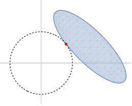
Figure 1. The numerical range from Example 2.3 and $z\in\mathcal{W}(C)$ minimizing $|z|$.

2.3. Complexity results for the Crawford number

A polynomial-time bit complexity (Turing complexity) of the SDP problem (1.4) using the ellipsoid method was shown by Grötschel-Lovász-Schrijver [5], under certain conditions, that are stated below. It used the ellipsoid method of Yudin-Nemirovski [16], and was inspired by the earlier proof of Khachiyan [9] of the polynomial-time solvability of linear programming.

Let $\mathrm{B}(G,r)=\{Y\in\mathbb{R}^{m\times m}:\|Y-G\|_{F}\leq r\}$ denote the ball of radius $r\geq 0$ centered at $G\in\mathbb{R}^{m\times m}$. The assumptions of Grötschel-Lovász-Schrijver [5] for the SDP (1.4) are:

(2.7) (1) $$F_{0},\ldots,F_{k}\in\mathbb{Q}^{m\times m},\ b_{1},\ldots,b_{k}\in\mathbb{Q}$$

(2) There exists $$G\in\mathcal{F}\cap\mathbb{Q}^{m\times m} G\succ 0 0<r\leq R$$ with and such that

$$\mathrm{B}(G,r)\cap\mathcal{L}(F_{1},b_{1},\ldots,F_{k},b_{k})\subseteq\mathcal{F}\subseteq\mathrm{B}(G,R)\cap\mathcal{L}(F_{1},b_{1},\ldots,F_{k},b_{k}).$$

Then the ellipsoid algorithm finds $X\in\mathcal{F}\cap\mathbb{Q}^{m\times m}$, such that $\langle F_{0},X\rangle\leq p^{\star}+\varepsilon$ [1, Theorem 1.1]. The complexity of the ellipsoid algorithm is polynomial in the bit sizes of $G,F_{0},\ldots,F_{k}$, $|\log\varepsilon|$ and $\log\frac{R}{r}$. Hence, for polynomial-time complexity of $\kappa(C)$ we need to assume that $C\in\mathbb{Q}[\mathbbm{i}]^{n\times n}$, which occurs if and only if $\widehat{C}\in\mathbb{Q}^{(2n)\times(2n)}.$

It was shown by Karmakar [8] that an IPM is superior to the ellipsoid method for linear programming problems. de Klerk-Vallentin [1, Theorem 7.1] showed polynomial-time complexity for an SDP problem using IPM method by applying the short step primal interior point method combined with Diophantine approximation under the above conditions.

Clearly, if $C$ is the zero matrix, then $\kappa(C)=0$. Hence we can assume that $n\geq 2$ and $C\neq 0$. We claim that we can assume that $\widehat{C}\in\mathbb{Z}^{(2n)\times(2n)}\setminus\{0\}$, i.e., $C\in\mathbb{Z}[\mathbbm{i}]$. Indeed, let $\ell\geq 1$ be the products of all denominators (viewed as positive integers) of the rational entries of $\widehat{C}\neq 0$. Let $\tilde{C}=\ell\widehat{C}$. Then $\kappa(\widehat{C})=\frac{1}{\ell}\kappa(\tilde{C})$. The following theorem gives an SDP characterization for which we can apply the poynomial-time complexity of $\kappa(C)$.

Theorem 2.4.

Let $C\in\mathbb{Q}[\mathbbm{i}]^{n\times n}\setminus\{0\}$ and $n\geq 2$. Let $(1/n)\operatorname{Tr}(C)=x+\mathbbm{i}y$ where $x,y\in\mathbb{R}$. The SDP (2.6) computing $\kappa(C)$ satisfies (2.7) with $r=1/n$, $R=12+4\lceil\|C\|_{F}\rceil$ and

(2.8) $$G=\operatorname{diag}\left(\tfrac{1}{n}I_{2n},S,1\right)\text{ where }S=\begin{bmatrix}\lceil\|C\|_{F}\rceil+1+x&y\\ y&\lceil\|C\|_{F}\rceil+1-x\end{bmatrix}.$$

In particular, if $C\in\mathbb{Z}[\mathbbm{i}]^{n\times n}$ then the ellipsoid method, or the IPM using the short step primal interior point method combined with Diophantine approximation, imply that the Turing complexity of $\varepsilon$-approximation of $\kappa(C)$ is polynomial in $n$, the bit sizes of the entries of $C$, and $|\log\varepsilon|$.

Proof.

We write $C=A+\mathbbm{i}B\in\mathbb{Q}[\mathbbm{i}]^{n\times n}$ where $A,B$ are Hermitian. The entries of $A,B$ also belong to $\mathbb{Q}[\mathbbm{i}]$ and the entries of $\widehat{A},\widehat{B}$ belong to $\mathbb{Q}$. Since the entries of $F_{1},\ldots,F_{N}$ were chosen to have entries in $\{-1,0,1\}$, all of the matrices $F_{0},\ldots,F_{N+4}$ used in (2.6) belong to $\mathbb{Q}^{(2n+3)\times(2n+3)}$, showing that assumption (1) of (2.7) is satisfied.

We take $x$, $y$, $r$, $R$, $S$, and $G$ as in the statement of the theorem and let

$$\mathcal{L}=\mathcal{L}(F_{1},0,\ldots,F_{N+2},0,F_{N+3},2,F_{N+4},2(\lceil\|C\|_{F}\rceil+2))$$

denote the affine linear subspace from (2.6).

First we claim that $G\succ 0$. For this, it suffices to show that $S\succ 0$. Note that $X=\frac{1}{n}I_{n}$ is positive definite and satisfies $\langle I_{n},X\rangle=1$. Therefore $x+\mathbbm{i}y=\frac{1}{n}\operatorname{Tr}C=\langle C,X\rangle\in\mathcal{W}(C)$. It follows that $|x+\mathbbm{i}y|\leq r(C)\leq\|C\|_{F}$. In particular, $\|C\|_{F}\pm x\geq 0$ and $x^{2}+y^{2}\leq\|C\|_{F}^{2}$, showing that the diagonal entries and determinant of $S-I_{2}$ are nonnegative. It follows that $S-I_{2}\succeq 0$ and thus $S\succeq I_{2}\succ 0$.

We next show that $\mathrm{B}(G,\frac{1}{n})\cap\mathcal{L}\subset\mathcal{F}$. Let $Z\in\mathrm{B}(G,\frac{1}{n})\cap\mathcal{L}$. It suffices to show that $Z\succeq 0$. Since $\mathcal{L}\subset\mathrm{H}_{2n}(\mathbb{R})\oplus\mathrm{H}_{2}(\mathbb{R})\oplus\mathrm{H}_{1}(\mathbb{R})$,

(2.9) $$Z=G+W \text{ where }W=\operatorname{diag}(W_{1},W_{2},W_{3})\in\mathrm{H}_{2n}(\mathbb{R})\oplus\mathrm{H}_{2}(\mathbb{R})\oplus\mathrm{H}_{1}(\mathbb{R})$$

$$\text{ with }\|W\|_{F}^{2}=\|W_{1}\|_{F}^{2}+\|W_{2}\|_{F}^{2}+\|W_{3}\|_{F}^{2}\leq(1/n)^{2}.$$

In particular $\|W_{j}\|_{F}\leq 1/n$ for each $j=1,2,3$. Note that the block diagonal matrix $Z$ is positive semidefinite if and only if each of its blocks, $\frac{1}{n}I_{2n}+W_{1}$, $S+W_{2}$ and $1+W_{3}$, are.

For any matrix $M\in\mathrm{H}_{m}(\mathbb{R})$, the Frobenius norm $\|M\|_{F}$ bounds the magnitude of all eigenvalues of $M$. In particular, if $\|M\|_{F}\leq\mu$, then $\mu I_{m}+M\succeq 0$. It follows that

$$\tfrac{1}{n}I_{2n}+W_{1}\succeq 0,\ \ S+W_{2}\succeq I_{2}+W_{2}\succeq 0,\ \text{ and }\ 1+W_{3}\succeq 0.$$

For the second inequality, we use that $S\succeq I_{2}$ as shown above. Thus $Z\succeq 0$.

We now show that $\mathcal{F}\subseteq\mathrm{B}(G,R)$. To do this, we use the trace of a positive semidefinite matrix to bound its Frobenius norm. For any matrix $M\in\mathrm{H}_{m,+}(\mathbb{R})$ and $\operatorname{Tr}(M)=\sum_{i=1}^{m}\lambda_{i}(M)$. Since $\|M\|_{F}^{2}=\sum_{i=1}^{m}\lambda_{i}^{2}(M)$ and $\lambda_{i}(M)\geq 0$ we find that

$$(\operatorname{Tr}(M))^{2}-\|M\|_{F}^{2}=\sum_{i\neq j}\lambda_{i}(M)\lambda_{j}(M)\geq 0.$$

In particular, $\|M\|_{F}\leq\operatorname{Tr}(M)$. Now suppose that $Z=\operatorname{diag}\left(Y,\begin{bmatrix}u&v\\ v&w\end{bmatrix},t\right)\in\mathcal{F}$. Then

$$\operatorname{Tr}(Z)=\operatorname{Tr}(Y)+u+w+t\leq 2+u+w+2t=6+2\lceil\|C\|_{F}\rceil.$$

Here we use the constraints $\operatorname{Tr}(Y)=\langle I_{n},Y\rangle=2$, $t\geq 0$ and $u+w+2t=2(\lceil\|C\|_{F}\rceil+2)$. By the arguments above, $\|Z\|_{F}\leq 6+2\lceil\|C\|_{F}\rceil$. Similarly, $G\in\mathcal{F}$ and so $\|G\|_{F}\leq 6+2\lceil\|C\|_{F}\rceil$. Then by the triangle inequality

$$\|Z-G\|_{F}\leq\|Z\|_{F}+\|G\|_{F}\leq 12+4\lceil\|C\|_{F}\rceil=R.$$

Therefore $\mathcal{F}\subset\mathrm{B}(G,R)$.

Assume that $C\in\mathbb{Z}[\mathbbm{i}]$. Clearly, $\frac{1}{n}\operatorname{Tr}C\in\mathbb{Q}[\mathbbm{i}]$. Hence, $G\in\mathbb{Q}^{(2n)\times(2n)}.$ The ellipsoid method, or the IPM using the short step primal interior point method combined with Diophantine approximation, imply that the Turing complexity of $\varepsilon$-approximation of $\kappa(C)$ is polynomial in $n$, the bit sizes of the entries of $C$, and $|\log\varepsilon|$. ∎

This theorem shows that $\kappa(C)$ can be computed using the standard software for SDP problems. This is also the case for the numerical radius and its dual norm, as pointed out in [4]. In numerical simulations in [12] it was shown that the known numerical methods for computing $r(A)$ are faster then the SDP methods. We suspect that the recent numerical methods in [11] for computing the Crawford number are superior to the SDP methods applied to the characterizations of the Crawford number discussed in this paper.

References

- [1] E. de Klerk and F. Vallentin, On the Turing model complexity of interior point methods for semidefinite programming, SIAM J. Optim. 26 (3), 2016, 1944–1961.
- [2] S. Friedland, Matrices: Algebra, Analysis and Applications, World Scientific, 596 pp., 2015, Singapore, http://www2.math.uic.edu/friedlan/bookm.pdf
- [3] S. Friedland, On semidefinite programming characterizations of the numerical radius and its dual norm for quaternionic matrices, arXiv:2311.01629, 2023.
- [4] S. Friedland and C.-K. Li, On a semidefinite programming characterizations of the numerical radius and its dual norm, arXiv:2308.07287, 2023.
- [5] M. Grötschel, L. Lovász and A. Schrijver, The ellipsoid method and its consequences in combinatorial optimization, Combinatorica 1 (1981), no. 2, 169-197.
- [6] D. Henrion, Semidefinite geometry of the numerical range, Electron. J. Linear Algebra 20 (2010), 322–332.
- [7] R. A. Horn and C. R. Johnson, Topics in Matrix Analysis, Cambridge University Press, Cambridge, UK, 1991.
- [8] N. Karmarkar, A new polynomial-time algorithm for linear programming, Combinatorica 4 (4) (1984), 373-395.
- [9] L. Khachiyan, A polynomial time algorithm in linear programming, Soviet Math. Dokl., 20 (1979), 191-194.
- [10] R. Kippenhahn, Über den Wertevorrat einer Matrix, Math. Nachr., 6:193-228, 1951.
- [11] D. Kressner, D. Lu, and B. Vandereycken, Subspace acceleration for the Crawford number and related eigenvalue optimization problems, SIAM J. Matrix Anal. Appl. 39 (2018), no. 2, 961-982.
- [12] T. Mitchell and M. L. Overton, An Experimental Comparison of Methods for Computing the Numerical Radius, arXiv:2310.04646.
- [13] Yu. Nesterov and A. S. Nemirovski, Interior-Point Polynomial Algorithms in Convex Programming, Stud. Appl. Math., SIAM, Philadelphia, 1994.
- [14] J. Renegar, A Mathematical View of Interior-Point Methods, in Convex Optimization, MOS-SIAM Ser. Optim., SIAM, Philadelphia, 2001.
- [15] L. Vandenberghe and S. Boyd, Semidefinite Programming, SIAM Review 38, March 1996, pp. 49-95.
- [16] D. Yudin and A. S. Nemirovski, Informational complexity and effective methods of solution of convex extremal problems, Econom. Math. Methods, 12 (1976), 357-369.