Actor-Critic Physics-informed Neural Lyapunov Control

Abstract

Designing control policies for stabilization tasks with provable guarantees is a long-standing problem in nonlinear control. A crucial performance metric is the size of the resulting region of attraction, which essentially serves as a robustness “margin” of the closed-loop system against uncertainties. In this paper, we propose a new method to train a stabilizing neural network controller along with its corresponding Lyapunov certificate, aiming to maximize the resulting region of attraction while respecting the actuation constraints. Crucial to our approach is the use of Zubov’s Partial Differential Equation (PDE), which precisely characterizes the true region of attraction of a given control policy. Our framework follows an actor-critic pattern where we alternate between improving the control policy (actor) and learning a Zubov function (critic). Finally, we compute the largest certifiable region of attraction by invoking an SMT solver after the training procedure. Our numerical experiments on several design problems show consistent and significant improvements in the size of the resulting region of attraction.

I Introduction

Neural network control policies have shown great promise in model-based control and outperformed existing design methods or even humans, owing to their capability to capture intricate nonlinear policies [1] [2] [3] [4]. For example, neural network control policies trained with reinforcement learning algorithms have been able to outperform human champions in drone racing [4]. Despite the outstanding empirical performance, the application of neural network policies in physical systems is of concern due to a lack of stability and safety guarantees.

Certificate functions such as Lyapunov functions provide a general framework to design nonlinear control policies with provable guarantees. For example, a quadratic Lyapunov function can be found with Linear Quadratic Regulator (LQR) [5] for a linear system, and a polynomial Lyapunov function can be found with Sum-of-Square (SoS) optimization [6] for a polynomial system. However, there is generally no universal way to construct these certificates for general nonlinear systems as it usually requires a predefined function form derived from the structure of the dynamical system.

Along with the development of neural networks as universal function approximators, there have been learning-based methods to construct Lyapunov functions represented by neural networks. The main focus is on either learning a Lyapunov function for an autonomous system [7][8][9] or co-learning a neural network control policy together with a neural Lyapunov function [10] [11] [12]. In these learning-based methods, a typical approach is to minimize the empirical violation of the Lyapunov conditions over the parameters of the controller and/or the certificate. Compared to optimization-based methods such as LQR and SoS, learning-based methods can be applied to more general non-linear systems beyond linear and polynomial systems.

However, in these learning-based methods, the Lyapunov conditions are only guaranteed at the sampled states. Thus there must be a verification procedure after the learning process to certify that the Lyapunov conditions are satisfied over a region. This verification is typically done by using Satisfiability Modulo Theories (SMT) solvers [13]. If the Lyapunov conditions are satisfied over a sub-level set of the neural Lyapunov function, then the learned function is a valid Lyapunov function over the sub-level set and the sub-level set is a domain of attraction (DoA). This brings us to another problem: how to learn a neural network control policy such that the certified region is maximized. Existing learning-based methods usually fail to obtain a large DoA as the loss function is not informed of this objective explicitly, leading to a shape mismatch between the level sets of the learned neural Lyapunov function and that of the true DoA.

Our Contribution

In this paper, we propose an algorithmic framework for learning a neural network control policy and a neural network Lyapunov function for actuation-constrained nonlinear systems. Our starting point is to use a physics-informed loss function based on Zubov’s Partial Differential Equation (PDE), the solution of which (the Zubov function) characterizes the true DoA. The framework follows an actor-critic pattern where we switch between learning a Zubov function and improving the control policy by minimizing its time derivative. By minimizing the PDE residual, the Our numerical experiments on several stabilization tasks show that our approach can enlarge the DoA significantly compared to the state-of-the-art approaches. The source code is available at https://github.com/bstars/ZubovControl

I-A Related Work

Learning Lyapunov Functions

There is a large body of work on learning Lyapunov functions for autonomous systems [7] [8] [9] [14]. In the work of Abate et al [7], they proposed a counter-example guided framework to learn a neural Lyapunov function. The algorithm switches between minimizing the violation of Lyapunov conditions at some sampled points and using an SMT solver to either verify the Lyapunov conditions or falsify them by counter-examples that are added to the training set. A common feature of these methods is that the level set of the learned Lyapunov function does not match the true DoA, leading to a conservative estimation of the DoA despite using neural networks. To capture the maximum region of attraction, Liu et al [15] mapped an easily constructed Lyapunov function, the time integration of the norm of the state along a trajectory, which is a true Lyapunov function in nature, to a Zubov function and learned a neural Zubov function with a physics-informed neural network. The result showed that this method approximately captures the maximum region of attraction. Our method also utilizes Zubov’s equation to co-learn the control policy and the stability certificate.

Co-learning Lyapunov Functions and Policies

This work is also built upon existing works on co-learning Lyapunov functions and control policies. Chang et al [10] proposed a counter-example guided method similar to [7] to co-learn a Lyapunov function and a control policy that jointly satisfy the Lyapunov conditions for nonlinear systems. In their work, they add a regularizer to the loss function to enlarge the DoA. The method in [10] has also been extended to safety certificates [11], unknown nonlinear systems [12] and discrete-time systems [16]. In our method, a regularizer is unnecessary as the Zubov equation itself captures the true DoA.

Actor-critic and Policy Iteration

Our framework is also inspired by the actor-critic method [17] [18] in reinforcement learning. Actor-critic methods consist of a control policy and a critic that evaluates the value function of the policy. Then the algorithm switches between evaluating the current policy and improving the policy by maximizing the value function.

Actor-critic methods can be seen as an approximation of policy iteration [18]. There have also been works that combine neural Lyapunov functions with policy iteration to learn formally verifiable control policies. In the work of [19], they use policy iteration to learn a control policy for a control-affine system. The policy evaluation part is done by representing the value function by a physics-informed neural network and minimizing the violation of the Generalized Hamilton-Jacobi-Bellman equation [20], and the policy improvement is done by minimizing the value function. Our method also follows a policy-evaluation-policy-improvement paradigm as in actor-critic method and policy iteration.

The rest of the paper is organized as follows. In $\S$II, we will provide background and formally state the problem. In $\S$III, we describe how to co-learn a control policy and a Lyapunov function with a physics-informed neural network and the verification procedure after training. In $\S$IV, we provide numerical experiments.

I-B Notation

We denote $n$-dimensional real vectors as $\mathbb{R}^{n}$. For $x\in\mathbb{R}^{n}$, $\|x\|$ denotes the Euclidean norm. $[x_{1},...,x_{n}]$ represents a matrix with columns $x_{1},...,x_{n}$. For a set $\mathcal{A}$, $\partial\mathcal{A}$ denotes the boundary of $\mathcal{A}$ and $\mathcal{A}\setminus\{0\}$ denotes the set $\mathcal{A}$ excluding the single point $0$. For a vector $x\in\mathbb{R}^{n}$, we use the notation $(x)_{+}=\max(x,0)$. $\mathbf{sg}(\cdot)$ stands for “stop gradient”, meaning that the argument in $\mathbf{sg}(\cdot)$ operator is treated as constant. (e.g., $\frac{d}{dx}(x\cdot\mathbf{sg}(ax))=ax$.

II Background and Problem Statement

II-A Lyapunov Certificates

Consider the autonomous nonlinear continuous-time dynamical system

$$\dot{x}=f(x)$$ (1)

where $x\in\mathcal{D}\subseteq\mathbb{R}^{n}$ is the state and $f\colon\mathcal{D}\to\mathbb{R}^{n}$ is a Lipschitz continuous function. For an initial condition $x_{0}\in\mathcal{D}$, we denote the unique solution by $x(t;x_{0})$, which we assume exists for all $t\geq 0$. Without loss of generality, we assume that the origin is an equilibrium of the system, $f(0)=0$.

Definition 1 (Asymptotic Stability[21])

The zero solution $x(t)=0$ to (1) is (locally) asymptotically stable if there exists a $\delta>0$ such that if $\|x_{0}\|<\delta$, then $\lim_{t\to\infty}x(t;x_{0})=0$

Definition 2 (Domain of Attraction [21])

If the solution $x(t)=0$ to (1) is asymptotically stable, then the domain of attraction (DoA) is given by

$$\mathcal{A}:=\big{\{}x_{0}\in\mathcal{D}:\lim_{t\to\infty}\|x(t;x_{0})\|=0\big{\}}$$

A common way to certify the stability of an equilibrium and estimate the DoA is via Lyapunov functions.

Theorem 1 (Lyapunov Stability)

Consider the nonlinear dynamical system in (1). If there exists a continuously differentiable function $V\colon\mathcal{D}\rightarrow\mathbb{R}$ satisfying the following conditions

$$V(0)=0$$ (2a)

$$V(x)>0~{}\forall~{}x\in\mathcal{D}\setminus\{0\}$$ (2b)

$$\nabla V(x)^{\top}f(x)<0~{}\forall x\in\mathcal{D}\setminus\{0\}$$ (2c)

then $x(t)=0$ is asymptotically stable. Furthermore, any sub-level set $\mathcal{D}_{\beta}=\{x:V(x)\leq\beta\}\subseteq\mathcal{D}$ containing the origin is a subset of the domain of attraction [21].

To find the maximum estimate of the domain of attraction, one must find the maximum $\beta$ such that $\mathcal{D}_{\beta}\subseteq\mathcal{D}$.

II-B Problem Statement

Consider the nonlinear continuous-time dynamical system

$$\dot{x}=f(x,u)$$ (3)

where $x\in\mathcal{D}\subseteq\mathbb{R}^{n}$ is the state, $u\in\mathcal{U}$ is the control input, $\mathcal{U}\subseteq\mathbb{R}^{m}$ is the actuation constraint set, and $f\colon\mathcal{D}\times\mathcal{U}\to\mathbb{R}^{n}$ is a Lipschitz continuous function. In this paper, we assume that $\mathcal{U}$ is a convex polyhedron.

Given a locally-Lipschitz control policy $\pi(\cdot)$ and an initial condition $x_{0}\in\mathbb{R}^{n}$, we denote the solution of the closed-loop system $\dot{x}=f(x,\pi(x))=f_{cl}(x)$ at time $t\geq 0$ by $x(t,x_{0};\pi)$.

In this paper, we are interested in learning a nonlinear control policy $\pi_{\gamma}(\cdot)$, parameterized by a neural network with trainable parameters $\gamma$, with the following desiderata:

• The control policy respects the actuation constraints, $\pi_{\gamma}(x)\in\mathcal{U}~{}\forall~{}x\in\mathcal{D}$;

• The zero solution of the closed-loop system $\dot{x}=f(x,\pi_{\gamma}(x))$ is asymptotically stable; and

• The domain of attraction of the equilibrium is maximized.

II-C Neural Lyapunov Control

A typical learning-enabled approach to designing stabilizing controllers is to parameterize the Lyapunov function candidate $V_{\theta}$ and the controller $\pi_{\gamma}$ with neural networks and aim to minimize the expected violation of Lyapunov conditions (2), i.e.,

$$\min_{\theta,\gamma}\!E_{x\sim\rho}\!\big{[}V_{\theta}(0)^{2}\!+\!(-V_{\theta}(x))_{+}\!+\!\big{(}\nabla_{x}V_{\theta}(x)^{\top}f(x,\pi_{\gamma}(x))\big{)}_{+}\big{]}$$ (4)

where $\rho$ is a predefined sampling distribution with support on $\mathcal{D}$ [10].

There are potentially infinitely many Lyapunov function candidates that minimize the expected loss, including the shortcut solution $V_{\theta}(x)=0~{}\forall x$. To avoid this shortcut and promote large domains of attractions, we must use regularization, e.g., $(\|x\|_{2}-\alpha V_{\theta}(x))^{2}$ [10]. However, poorly chosen regularizers can lead to a mismatch between the shape of level sets of the learned Lyapunov function and the true DoA. Motivated by this drawback, we will design a physics-informed loss function to directly capture the true DoA.

III Physics-Informed Actor-Critic Learning

III-A Maximal Lyapunov Functions and Zubov’s Method

To characterize the domain of attraction exactly, we can use a variation of the Lyapunov function, called the maximal Lyapunov function [22].

Theorem 2 (Maximal Lyapunov Function)

Suppose there exists a set $\mathcal{A}\subseteq\mathcal{D}$ containing the origin in its interior, a continuously differentiable function $V\colon\mathcal{A}\rightarrow\mathbb{R}$, and a positive definite function $\Phi$ satisfying the following conditions

$$V(0)=0,V(x)>0~{}\forall x\in\mathcal{A}\setminus\{0\}$$ (5a)

$$\nabla V(x)^{\top}f(x)=-\Phi(x)~{}\forall x\in\mathcal{A}$$ (5b)

$$V(x)\to\infty\text{ as }x\to\partial\mathcal{A}\text{ or }\|x\|\to\infty$$ (5c)

Then $\mathcal{A}$ is the domain of attraction.

One can verify that the function

$$V(x)=\begin{cases}\int_{0}^{\infty}\|x(t;x_{0})\|dt&\text{if the integral converges}\\ \infty&\text{otherwise}\end{cases}$$ (6)

satisfies the conditions of Theorem 2 with $\Phi(x)=\|x\|$ [22].

Due to the presence of infinity, the maximal Lyapunov function is hard to represent by function approximators such as neural networks. Another way to build a Lyapunov function and characterize the domain of attraction is using Zubov’s Theorem [21] [23].

Theorem 3 (Zubov’s Theorem [23])

Consider the nonlinear dynamical system in (1) with $f(0)=0$. Let $\mathcal{A}\subseteq\mathcal{D}$ and assume there exists a continuously differentiable function $W\colon\mathcal{A}\rightarrow\mathbb{R}$ and a positive definite function $\Psi:\mathbb{R}^{n}\rightarrow\mathbb{R}$ satisfying the following conditions,

$$W(0)=0$$ (7a)

$$0<W(x)<1~{}\forall x\in\mathcal{A}\setminus\{0\}$$ (7b)

$$W(x)\to 1\text{ as }x\to\partial\mathcal{A}$$ (7c)

$$\nabla W(x)^{\top}f(x)=-\Psi(x)(1-W(x)).$$ (7d)

Then the zero solution $x(t)=0$ is asymptotically stable with domain of attraction $\mathcal{A}$.

Intuitively, the Zubov PDE (7d) ensures that the Lie derivative of $W$ on the boundary of $\mathcal{A}$ is zero, a property which precisely renders $\mathcal{A}$ the domain of attraction–see Figure 1 for an illustration.

We note that the $V(\cdot)$ function in Theorem 2 and the $W(\cdot)$ function in Theorem 3 can be related by [24]

$$W(x) =\mathrm{tanh}(\alpha V(x))$$ (8a)

$$V(x) =\frac{1}{2\alpha}\log\big{(}\frac{1+W(x)}{1-W(x)}\big{)}$$ (8b)

$$\Psi(x) =\alpha(1+W(x))\Phi(x)$$ (8c)

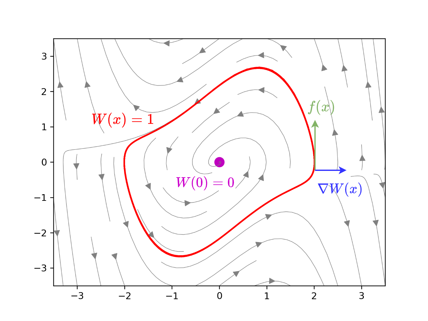
Figure 1: The level set $\{x:W(x)=1\}$ obtained by the Zubov PDE characterizes the boundary of the true DoA.

III-B Learning the Zubov Function (Critic)

Suppose we have a fixed policy $\pi_{\gamma}(\cdot)$ and the corresponding closed-loop system $\dot{x}=f(x,\pi_{\gamma}(x))$. Let $V(\cdot)$ be chosen as in (6). The relationship (8a), combined with (7d), enables us to learn the neural Zubov function $W_{\theta}(x)\approx\mathrm{tanh}(\alpha V(x))$, which can be interpreted as an evaluation of the policy $\pi_{\gamma}$. To this end, we use the following loss function

$$L(\theta)=L_{z}(\theta)+L_{r}(\theta)+L_{p}(\theta)$$ (9)

where

$$L_{z}(\theta) =W_{\theta}(0)^{2}$$ (10a)

$$L_{r}(\theta) =\frac{1}{M}\sum_{i=1}^{M}\big{(}W_{\theta}(x_{i})-\mathrm{tanh}(\alpha V(x_{i})\big{)}^{2}$$ (10b)

$$L_{p}(\theta) =\frac{1}{K}\sum_{i=1}^{K}\bigg{[}\nabla_{x}W_{\theta}(x_{i})^{\top}f(x_{i},\pi(x_{i}))+$$ (10c)

$$\qquad\qquad\alpha(1-W_{\theta}(x_{i}))(1+W_{\theta}(x_{i}))\Phi(x)\bigg{]}^{2}$$

Here $W_{\theta}(\cdot)$ is a neural network with $\mathrm{tanh}$ activation functions at the output layer [25] such that $W_{\theta}(x)\in(0,1)\forall x\in\mathcal{D}$. The first term $L_{z}(\theta)$ penalizes the violation of the condition (7a). The second term $L_{r}(\theta)$ penalizes the violation of the relationship (8a). To evaluate $V(\cdot)$ that appears in this loss, we must simulate the closed-loop system from the initial conditions $\{x_{i}\}_{i=1}^{M}$. Finally, the third term $L_{p}(\theta)$ is the physic-informed part to minimize the residual of the Zubov PDE in (7d).

III-C Policy Improvement (Actor)

Given a policy $\pi_{\gamma}(\cdot)$, the corresponding Zubov function is $W(x)=\tanh(\alpha V^{\pi_{\gamma}}(x))$ where $V^{\pi_{\gamma}}(x)$ is defined as in (6). We can improve the policy to drive the state to $x=0$ by minimizing the time derivative $\dot{W}(x)$. However, since we cannot differentiate $W(x)$ with respect to $x$, we use $W_{\theta}(\cdot)$ as a proxy of the true $W$, which results in the following loss function

$$L_{c}(\gamma)=\frac{1}{K}\sum_{i=1}^{K}\bigg{[}\frac{\nabla_{x}W_{\theta}(x_{i})^{\top}}{\|\nabla_{x}W_{\theta}(x_{i})\|}f(x_{i},\pi_{\gamma}(x_{i}))\bigg{]}$$

Here we normalize the gradient $\nabla_{x}W_{\theta}(x)$ so that the training samples are equally weighted in both the steep regions and flat regions of $W_{\theta}(\cdot)$.

III-D Actor-Critic Learning

We now combine the critic of $\S$III-B and the actor of $\S$III-C to co-learn the controller and the Zubov function. We first define $R_{1}\subseteq\mathcal{D}$ to be the region from which we sample $\{x_{i}\}$ and define the region $R_{2}=\{ax:x\in R_{1}\}$ ($a>0$) as the region of interest. Since the controller is randomly initialized, the sampled trajectories might diverge. To prevent this, we add a barrier-like loss function [26] as follows,

$$L_{b}(\theta)=\frac{1}{K}\sum_{x^{\prime}_{i}\in\partial R_{2},i=1,...,K}\big{|}W_{\theta}(x^{\prime}_{i})-1\big{|}$$

This loss function stabilizes the training at the beginning.

Combining policy evaluation and policy improvement, we can co-learn a controller and a Zubov function in an actor-critic fashion by minimizing the following loss function

$$L(\theta,\gamma) =\lambda_{0}W_{\theta}(0)^{2}$$ (11)

$$~{}~{}+\frac{1}{M}\sum_{x_{i}\in R_{1},i=1,..,M}\big{(}W_{\theta}(x_{i})-\mathrm{tanh}(\alpha V(x_{i})\big{)}^{2}$$

$$~{}~{}+\frac{1}{K}\sum_{x_{i}\in R_{1},i=1,..,K}\bigg{[}\nabla_{x}W_{\theta}(x_{i})^{\top}f(x_{i},\mathbf{sg}(\pi_{\gamma}(x_{i}))$$

$$~{}~{}~{}~{}~{}~{}~{}~{}~{}~{}~{}~{}~{}~{}~{}~{}~{}~{}+\alpha(1-W_{\theta}(x_{i}))(1+W_{\theta}(x_{i}))\Phi(x)\bigg{]}^{2}$$

$$~{}~{}+\frac{\lambda_{c}}{K}\sum_{x_{i}\in R_{1},i=1,..,K}\bigg{[}\mathbf{sg}(\frac{\nabla_{x}W_{\theta}(x_{i})^{\top}}{\|\nabla_{x}W_{\theta}(x_{i})\|})f(x_{i},\pi_{\gamma}(x_{i}))\bigg{]}$$

$$~{}~{}+\frac{\lambda_{b}}{K}\sum_{x^{\prime}_{j}\in\partial R_{2},j=1,...,K}\big{|}W_{\theta}(x^{\prime}_{j})-1\big{|}$$

where $M$ is the number of trajectories sampled at each iteration, $K$ is the batch size. Note that rather than alternating between updating $W_{\theta}(\cdot)$ and $\pi_{\gamma}(\cdot)$ with the other one fixed, are use the $\mathbf{sg(\cdot)}$ operator to enable a simultaneous update of $W_{\theta}(\cdot)$ and $\pi_{\gamma}(\cdot)$. We outline the overall method in 1.

Algorithm 1 Physics-Informed Neural Lyapunov Control

Randomly initialize $W_{\theta}$ and $\pi_{\gamma}$

for $n=1,...,T$ do

     Randomly sample $x_{1},...,x_{K}$ from $R_{1}$

     Randomly sample $x^{\prime}_{1},...x^{\prime}_{K}$ from $\partial R_{2}$

     Simulate trajectories $x(t,x_{i};\pi_{\gamma})$ (with RK-4 integrator)

     Estimate $V(x_{i})\approx\int_{t}\|x(t,x_{i};\pi)\|dt$

     Take a gradient step to minimize $L(\theta,\gamma)$ in (11)

end for

III-E Actuation Constraints

To respect actuation constraints, one approach is to append a Euclidean projection layer to a generic neural network $u_{\gamma}(\cdot)$, resulting in the control policy

$$\pi_{\gamma}(x)=\mathrm{Proj}_{\mathcal{U}}[u_{\gamma}(x)]=\mathrm{argmin}_{u^{\prime}\in\mathcal{U}}\|u^{\prime}-u_{\gamma}(x)\|_{2}^{2}$$ (12)

For convex $\mathcal{U}$, we can compute the derivative $D_{\gamma}u_{\gamma}(x)$, which is needed to learn $\gamma$, using differentiable convex optimization layers [27]. This approach is particularly efficient for box constraint sets, $\mathcal{U}=\{u:\underline{u}\leq u\leq\bar{u}\}$, for which the projection can be computed in closed form. However, for general convex polyhedrons, the projection has to be solved numerically. To avoid this, our innovative solution is to span the actuation constraint set $\mathcal{U}$ using a convex combination of its vertices. Formally, suppose $V=[v_{1}\ \cdots v_{M}]$ is the matrix of vertices of $\mathcal{U}$. We then parameterize the control policy as

$$\pi_{\gamma}(x)\!=\!V\cdot\mathrm{softmax}(u_{\gamma}(x))\!=\!\sum_{i=1}^{M}V_{i}\cdot\mathrm{softmax}(u_{\gamma}(x))_{i}$$ (13)

where the vector-valued softmax function simply generates the coefficients of the convex combination of columns of $V$ and $u_{\gamma}(\cdot)$ is a neural network. In contrast to (12), this parameterization eliminates the need to compute any numerical optimization sub-routine.

III-F Verification

By minimizing the empirical loss over the sampled states, the learned controller is not guaranteed to be stabilizing, thus we need to formally verify the learned certificate function.

Let $c$ be a real number between $0$ and $1$, we attempt to verify the following three conditions

$$\begin{cases}W_{\theta}(x)>W_{\theta}(0)~{}\forall x\in R_{2},W_{\theta}(x)<c,\|x\|\geq\epsilon\\ \dot{W}_{\theta}(x)<0~{}\forall x\in R_{2},W_{\theta}(x)<c,\|x\|\geq\epsilon\\ W_{\theta}(x)>c~{}\forall x\in\partial R_{2}\end{cases}$$ (14)

Because of the complexity of neural network functions, a sublevel set may consist of multiple disjoint sets, we only consider the sublevel set in the region of interest. The first and second conditions verify the Lyapunov condition on the set $\mathcal{D}=R_{2}\cap\{x:W_{\theta}(x)<c\}$. We ignore a smaller neighbor around the origin to avoid numerical errors. However, the first two conditions do not imply that $\mathcal{D}$ is the domain of attraction. We also need to verify the third condition, which implies that the set $\mathcal{D}$ is strictly contained in $R_{2}$ so that a trajectory does not leave $R_{2}$ with negative $\dot{W}_{\theta}$ along the trajectory. If these two conditions are satisfied, then the function $W_{\theta}(x)-W_{\theta}(0)$ is a Lyapunov function in the region $R_{2}\cap\{x:W_{\theta}(x)<c\}$.

IV Numerical Experiments

We demonstrate the effectiveness of our method on various nonlinear control problems. We first run our method on Double Integrator and Van der Pol and compare the verified DoA obtained by our method with that of the LQR controller. We then test our method on Inverted Pendulum and Bicycle Tracking and compare it to both LQR and Neural Lyapunov Control [10]. Across all examples, we use the same hyperparameter $M=8,K=64,\lambda_{0}=5,\lambda_{c}=0.5$, and $\lambda_{b}=5$ for the loss function. Other hyperparameters can be found in Table I. In all experiments, we assumed that the actuation constraint is $u\in\mathcal{U}=\{u|~{}\|u\|_{\infty}\leq 1\}$ and the learned controller satisfies this constraint by using $\mathrm{tanh}$ as the activation function in the output layer.

To find the DoA of LQR under actuation constraints, we first solve the Riccati equation of the linearized system with $Q=I,R=I$ to obtain the solution $P$ and control matrix $K$, and then we verify the following conditions

$$x^{\top}P\dot{x}<0\text{ and }\|Kx\|_{\infty}\leq 1~{}\forall x^{\top}Px<c_{lqr},\|x\|\geq\epsilon$$ (15)

by an SMT solver, where $\dot{x}$ is given by the nonlinear closed-loop dynamics. To find the largest DoA, we perform bisection to find the largest $c_{lqr}$ such that both conditions are satisfied.

We used the SMT solver dReal [28] to verify the conditions (14) for the neural network controller and (15) for the LQR controller.

IV-A Double Integrator

We first consider the double integrator dynamics,

$$\begin{bmatrix}\dot{x}_{1}\\ \dot{x}_{2}\end{bmatrix}=\begin{bmatrix}x_{2}\\ u\end{bmatrix}$$

The learned Lyapunov function is shown in Figure 2(a). The verified DoA and the vector field induced by the learned controller are shown in Figure 2(b).

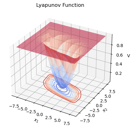
(a) $W_{\theta}(x)$ learned for double integrator system

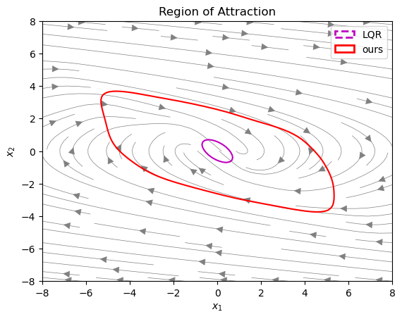
(b) Verified DoA and vector field $\dot{x}=f(x,\pi_{\gamma}(x))$

Figure 2: Double integrator system

IV-B Van der Pol

Consider the Van der Pol system

$$\begin{bmatrix}\dot{x}_{1}\\ \dot{x}_{2}\end{bmatrix}=\begin{bmatrix}x_{2}\\ x_{1}-\mu(1-x_{1}^{2})x_{2}+u\end{bmatrix}$$

The learned Lyapunov function is shown in Figure 3(a). The verified DoA and the vector field induced by the learned controller are shown in Figure 3(b).

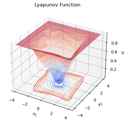
(a) $W_{\theta}(x)$ learned for Van der Pol system

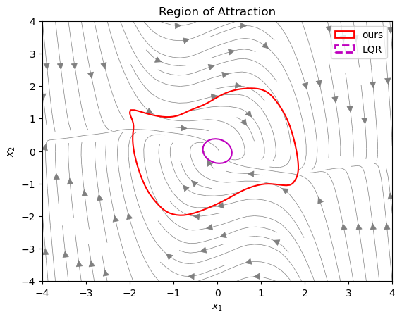
(b) Verified DoA and vector field $\dot{x}=f(x,\pi_{\gamma}(x))$

Figure 3: Van der Pol system

IV-C Inverted Pendulum

The inverted pendulum system has two states, the angular position $\theta$, angular velocity $\dot{\theta}$ and control input $u$. The dynamical system of inverted pendulum is

$$\begin{bmatrix}\dot{\theta}\\ \ddot{\theta}\end{bmatrix}=\begin{bmatrix}\dot{\theta}\\ \frac{g}{l}\sin(\theta)-\frac{b\dot{\theta}}{ml^{2}}+\frac{u}{ml^{2}}\end{bmatrix}$$

The learned Lyapunov function is shown in Figure 4(a). The verified DoA and the vector field induced by the learned controller are shown in Figure 4(b).

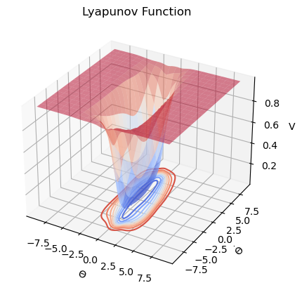
(a) $W_{\theta}(x)$ learned for inverted pendulum system

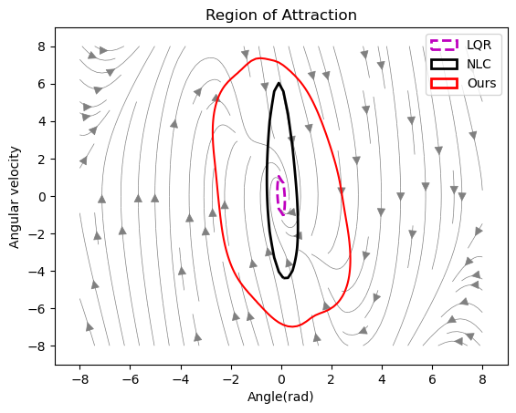
(b) Verified DoA and vector field $\dot{x}=f(x,\pi_{\gamma}(x))$

Figure 4: Inverted Pendulum system

IV-D Bicycle Tracking

The bicycle tracking system has two states, the distance $d_{e}$, angle error $\theta_{e}$, and control input $u$. The dynamical system for the tracking problem is

$$\begin{bmatrix}\dot{d}_{e}\\ \dot{\theta}_{e}\end{bmatrix}=\begin{bmatrix}v\sin(\theta_{e})\\ v\frac{\tan(u)}{l}-\frac{\cos(\theta_{e})}{1-d_{e}}\end{bmatrix}$$

The learned Lyapunov function is shown in Figure 5(a). The verified DoA and the vector field induced by the learned controller are shown in Figure 5(b).

(a) $W_{\theta}(x)$ learned for bicycle tracking system

(b) Verified DoA and vector field $\dot{x}=f(x,\pi_{\gamma}(x))$

Figure 5: Bicycle tracking system

All the experiments show that the verified DoA obtained by our method is 2$\sim$4 times larger than all other methods.

Dynamical System	$W_{\theta}$ dimension	$\pi_{\gamma}$ dimension	$\alpha$	$c$
Double Integrator	[2,20,20,1]	[2, 10, 10, 1]	0.05	0.7
Van der Pol	[2,30,30,1]	[2, 30, 30, 1]	0.1	0.5
Inverted Pendulum	[2, 20, 20, 1]	[2, 5, 5, 1]	0.2	0.7
Bicycle Tracking	[2, 20, 20, 1]	[2, 10, 10, 1]	1.5	0.4

TABLE I: Hyperparameters for each experiment

V CONCLUSIONS

In this paper, we developed an actor-critic framework to jointly train a neural network control policy and the corresponding stability certificate, with the explicit goal of maximizing the induced region of attraction. To this end, we leveraged Zubov’s partial differential equation to inform the loss function of the shape of the boundary of the true domain of attraction. Our numerical experiments on several nonlinear benchmark examples corroborate the superiority of the proposed method over competitive approaches in enlarging the domain of attraction. For future work, we will incorporate robustness to model uncertainty in our loss function. We will also investigate the extension of the proposed method to discrete-time systems [16].

References

- [1] S. Li, E. Öztürk, C. De Wagter, G. C. De Croon, and D. Izzo, “Aggressive online control of a quadrotor via deep network representations of optimality principles,” in 2020 IEEE International Conference on Robotics and Automation (ICRA), pp. 6282–6287, IEEE, 2020.
- [2] X. Yang, D. Liu, and Y. Huang, “Neural-network-based online optimal control for uncertain non-linear continuous-time systems with control constraints,” IET Control Theory & Applications, vol. 7, no. 17, pp. 2037–2047, 2013.
- [3] J. Zhang, Q. Zhu, and W. Lin, “Neural stochastic control,” Advances in Neural Information Processing Systems, vol. 35, pp. 9098–9110, 2022.
- [4] E. Kaufmann, L. Bauersfeld, A. Loquercio, M. Müller, V. Koltun, and D. Scaramuzza, “Champion-level drone racing using deep reinforcement learning,” Nature, vol. 620, no. 7976, pp. 982–987, 2023.
- [5] H. Kwakernaak and R. Sivan, Linear optimal control systems, vol. 1. Wiley-interscience New York, 1972.
- [6] A. A. Ahmadi and A. Majumdar, “Some applications of polynomial optimization in operations research and real-time decision making,” Optimization Letters, vol. 10, pp. 709–729, 2016.
- [7] A. Abate, D. Ahmed, M. Giacobbe, and A. Peruffo, “Formal synthesis of lyapunov neural networks,” IEEE Control Systems Letters, vol. 5, no. 3, pp. 773–778, 2020.
- [8] N. Gaby, F. Zhang, and X. Ye, “Lyapunov-net: A deep neural network architecture for lyapunov function approximation,” in 2022 IEEE 61st Conference on Decision and Control (CDC), pp. 2091–2096, IEEE, 2022.
- [9] L. Grüne, “Computing lyapunov functions using deep neural networks,” arXiv preprint arXiv:2005.08965, 2020.
- [10] Y.-C. Chang, N. Roohi, and S. Gao, “Neural lyapunov control,” Advances in neural information processing systems, vol. 32, 2019.
- [11] W. Jin, Z. Wang, Z. Yang, and S. Mou, “Neural certificates for safe control policies,” arXiv preprint arXiv:2006.08465, 2020.
- [12] R. Zhou, T. Quartz, H. D. Sterck, and J. Liu, “Neural lyapunov control of unknown nonlinear systems with stability guarantees,” 2022.
- [13] C. Barrett and C. Tinelli, Satisfiability modulo theories. Springer, 2018.
- [14] N. Boffi, S. Tu, N. Matni, J.-J. Slotine, and V. Sindhwani, “Learning stability certificates from data,” in Conference on Robot Learning, pp. 1341–1350, PMLR, 2021.
- [15] M. Raissi, P. Perdikaris, and G. E. Karniadakis, “Physics-informed neural networks: A deep learning framework for solving forward and inverse problems involving nonlinear partial differential equations,” Journal of Computational physics, vol. 378, pp. 686–707, 2019.
- [16] J. Wu, A. Clark, Y. Kantaros, and Y. Vorobeychik, “Neural lyapunov control for discrete-time systems,” Advances in Neural Information Processing Systems, vol. 36, 2024.
- [17] V. Konda and J. Tsitsiklis, “Actor-critic algorithms,” Advances in neural information processing systems, vol. 12, 1999.
- [18] R. S. Sutton, A. G. Barto, et al., “Introduction to reinforcement learning. vol. 135,” 1998.
- [19] Y. Meng, R. Zhou, A. Mukherjee, M. Fitzsimmons, C. Song, and J. Liu, “Physics-informed neural network policy iteration: Algorithms, convergence, and verification,” arXiv preprint arXiv:2402.10119, 2024.
- [20] R. Leake and R.-W. Liu, “Construction of suboptimal control sequences,” SIAM Journal on Control, vol. 5, no. 1, pp. 54–63, 1967.
- [21] W. M. Haddad and V. Chellaboina, Nonlinear Dynamical Systems and control: A Lyapunov-based approach. Princeton University, 2008.
- [22] A. Vannelli and M. Vidyasagar, “Maximal lyapunov functions and domains of attraction for autonomous nonlinear systems,” Automatica, vol. 21, no. 1, pp. 69–80, 1985.
- [23] V. I. Zubov, Methods of AM Lyapunov and their application, vol. 4439. US Atomic Energy Commission, 1961.
- [24] W. Kang, K. Sun, and L. Xu, “Data-driven computational methods for the domain of attraction and zubov’s equation,” IEEE Transactions on Automatic Control, 2023.
- [25] J. Liu, Y. Meng, M. Fitzsimmons, and R. Zhou, “Physics-informed neural network lyapunov functions: Pde characterization, learning, and verification,” arXiv preprint arXiv:2312.09131, 2023.
- [26] A. D. Ames, X. Xu, J. W. Grizzle, and P. Tabuada, “Control barrier function based quadratic programs for safety critical systems,” IEEE Transactions on Automatic Control, vol. 62, no. 8, pp. 3861–3876, 2016.
- [27] A. Agrawal, B. Amos, S. Barratt, S. Boyd, S. Diamond, and J. Z. Kolter, “Differentiable convex optimization layers,” Advances in neural information processing systems, vol. 32, 2019.
- [28] S. Gao, S. Kong, and E. M. Clarke, “dreal: An smt solver for nonlinear theories over the reals,” in Automated Deduction–CADE-24: 24th International Conference on Automated Deduction, Lake Placid, NY, USA, June 9-14, 2013. Proceedings 24, pp. 208–214, Springer, 2013.