How motility drives the glassy dynamics in confluent epithelial monolayers?
Abstract
As wounds heal, embryos develop, cancer spreads, or asthma progresses, the cellular monolayer undergoes a glass transition from a solid-like jammed to a fluid-like flowing state. Two primary characteristics of these systems, confluency, and self-propulsion, make them distinct from particulate systems. Are the glassy dynamics in these biological systems and equilibrium particulate systems different? Despite the biological significance of glassiness in these systems, no analytical framework, which is indispensable for deeper insights, exists. Here, we extend one of the most popular theories of equilibrium glasses, the random first-order transition (RFOT) theory, for confluent systems with self-propulsion. One crucial result of this work is that, unlike in particulate systems, the confluency affects the effective persistence time-scale of the active force, described by its rotational diffusion . Unlike in particulate systems, this value differs from the bare rotational diffusion of the active propulsion force due to cell shape dynamics which acts to rectify the force dynamics: is equal to when is small, and saturates when is large. We present simulation results for the glassy dynamics in active confluent models and find that the results are consistent with existing experimental data, and conform remarkably well with our theory. In addition, we show that the theoretical predictions agree nicely with and explain previously published simulation results. Our analytical theory provides a foundation for rationalizing and a quantitative understanding of various glassy characteristics of these biological systems.
I Introduction
The glassy nature of collective cellular dynamics in epithelial monolayers is crucial for many biological processes, such as embryogenesis Tambe et al. (2011); Friedl and Gilmour (2009); Malmi-Kakkada et al. (2018); Schötz et al. (2013), wound healing Poujade et al. (2007); Das et al. (2015); Brugués et al. (2014); Malinverno et al. (2017), cancer progression Streitberger et al. (2020); Friedl and Wolf (2003). One defining feature of glassiness is the rapid growth of relaxation time by several orders of magnitude, with a modest change in the control parameter Berthier and Biroli (2011); Pareek et al. (2023). This enormous dynamical slow-down does not seem to accompany any apparent structural change in the static properties. However, there are several dynamical signatures, such as complex non-exponential relaxation Angelini et al. (2011); Park et al. (2015), dynamical heterogeneity Nnetu et al. (2012); Park et al. (2015), caging Szabó et al. (2006), non-Gaussian particle displacements Trepat et al. (2009); Giavazzi et al. (2018); Atia et al. (2021). Although most of these glassy characteristics in biological systems are similar to those of non-living systems, there are crucial differences Paul et al. (2021, 2023). These systems are active, that is, driven out of equilibrium. Activity has many different forms; for example, the constituents of such systems can divide and die Prost et al. (2015); Ranft et al. (2010); Matoz-Fernandez et al. (2017), differentiate Alvarado and Yamanaka (2014), be confluent Farhadifar et al. (2007); Garcia et al. (2015), be motile and self-propel Ramaswamy (2010); Marchetti et al. (2013), etc. These properties are distinctive from those of non-living glassy systems and provide opportunities for fascinating discoveries and challenging theoretical directions.
The effects of motility on the glassy dynamics of particulate systems are relatively well-understood Janssen (2019); Berthier et al. (2019); Paoluzzi et al. (2022). These systems comprise self-propelled particles (SPPs) with a self-propulsion force, , that has characteristic persistence time, Ramaswamy (2010); Marchetti et al. (2013). The force persistence time leads to a separation of time scales between the thermal and active dynamics. When is not too large, an equilibrium-like description with an extended fluctuation-dissipation relation applies Palacci et al. (2010); Szamel (2014); Han et al. (2017); Fodor et al. (2016); Parisi (2005). Due to the inherent complexities of these systems, simulation studies Berthier (2014); Mandal et al. (2016); Flenner et al. (2016); Ni et al. (2013) and experiments on synthetic systems Klongvessa et al. (2019a, b); Arora et al. (2022) have provided crucial insights. Theories of equilibrium glasses, such as the mode-coupling theory (MCT) Berthier and Kurchan (2013); Szamel (2016); Flenner et al. (2016); Liluashvili et al. (2017); Feng and Hou (2017); Nandi and Gov (2017) or random first-order transition (RFOT) theory Nandi et al. (2018); Mandal et al. (2022), have been extended for active SPP systems. Surprisingly, many of the equilibrium glass properties survive in the presence of activity Berthier and Kurchan (2013); Berthier et al. (2019); Nandi and Gov (2017); Paul et al. (2023), and the relaxation dynamics remain equilibrium-like at an effective temperature when is not high. However, cellular monolayers and epithelial tissues, the systems of interest in this work, have a crucial difference from the particulate systems; they are confluent, that is, the particles fill the entire space and to date, no theory exists for the effect of motility on the glassy dynamics in such systems. Here, we develop a theoretical framework to understand how motility drives the glassy dynamics in confluent systems.
Several computational models exist to study the static and dynamical properties of confluent epithelial monolayers: for example, the cellular Potts model (CPM) Graner and Glazier (1992); Glazier and Graner (1993); Hogeweg (2000); Hirashima et al. (2017); Chiang and Marenduzzo (2016); Sadhukhan and Nandi (2021), the Vertex model Farhadifar et al. (2007); Honda and Eguchi (1980); Marder (1987); Fletcher et al. (2014), the Voronoi model Bi et al. (2016); Li et al. (2021); Czajkowski et al. (2019), the phase-field model Nonomura (2012); Palmieri et al. (2015); Loewe et al. (2020), etc. These models essentially vary in the details of implementations. Recent works have shown that all these models are similar from the perspective of the glassy dynamics, exhibiting a jamming transition from fluid-like fast dynamics to solid-like slow dynamics Bi et al. (2014, 2016); Sussman et al. (2018); Li et al. (2021); Sadhukhan and Nandi (2021). Note that this ‘jamming transition’ is distinct from the zero-temperature zero-activity jamming transition found in the physics of disordered systems Berthier et al. (2019); Atia et al. (2021); Sadhukhan and Nandi (2022) since here the jamming phenomenon essentially refers to the appearance of glassy dynamics. In confluent systems, the glassy dynamics have several unusual properties.
Compared to most particulate systems, confluent systems readily show sub-Arrhenius relaxation dynamics Sussman et al. (2018); Li et al. (2021); Sadhukhan and Nandi (2021), and cellular shape is a crucial control parameter for these systems Bi et al. (2016); Sadhukhan and Nandi (2022). These unusual properties make a theoretical description of the glassy properties in these systems challenging. In a recent work, some of us have phenomenologically extended one of the most popular theories of glassy dynamics, the random first-order transition (RFOT) theory Lubchenko and Wolynes (2007); Kirkpatrick and Thirumalai (2015); Biroli and Bouchaud (2012), for a confluent monolayer of cells (lacking self-propulsion) Sadhukhan and Nandi (2021). The theoretical predictions agree well with the simulation results of equilibrium CPM in the absence of motility. However, cells are inherently out of equilibrium, and motility is crucial for cellular dynamics. In a seminal work, Bi et al have studied a minimal self-propelled Voronoi model Bi et al. (2016) and showed that , and the typical cell shape crucially affect the glassy behavior in these systems Bi et al. (2016). Thus, including motility within the analytical RFOT-inspired framework for confluent systems is essential. Crucially, as we show below, confluency has non-trivial effect on self-propulsion leading to novel phenomenology for the relaxation dynamics.
In this work, we extend the RFOT theory framework to understand how motility affects the glassy dynamics in confluent epithelial monolayers. The main results of the work are as follows: (1) We show that confluency has a non-trivial effect on the self-propulsion; specifically, it modifies the effective persistence time of the active forces, such that they differ from the intrinsic . This is described by the modified rotational diffusivity arising from the coupling between shape and active force relaxation. (2) We extend the RFOT theory for confluent systems by adding the effects of self-propulsion and show that the theory agrees with our simulation results of active Vertex model. (3) We demonstrate that our extended RFOT theory rationalizes the existing simulation results for the active confluent systems and agrees quite well in determining the phase diagrams governing the glass transition from the solid-like jammed to fluid-like flowing state. These results illustrate that the effect of confluency on the self-propulsion is crucial for understanding how motility affects the glassy dynamics in confluent systems.
II Models for confluent cell monolayer
To set the notations, we first briefly describe the confluent models representing an epithelial monolayer. Experiments show that the height of a monolayer remains nearly constant Farhadifar et al. (2007). Thus, a two-dimensional description, representing cells as polygons, is possible Marder (1987); Weaire and Hutzler (2001); Albert and Schwarz (2016). The computational models have two parts: the energy function and the way in which cells are defined in the model. The energy function, , describing a cellular monolayer is
| (1) |
where is the total number of cells in the monolayer, and are the target area and target perimeter, respectively. and are the instantaneous area and perimeter of the th cell. and are area and perimeter moduli; they determine the strength with which the area and perimeter constraints in Eq. (1) are satisfied. The physical motivation behind the energy function, , is the following: We can treat the cell cytoplasm as an incompressible fluid Prost et al. (2015); therefore, the total cell volume is constant. Since the cellular heights in the monolayer remain nearly the same, cells want to have a preferred area, . can vary for different cells, but we have assumed it to be uniform for simplicity. On the other hand, is a coarse-grained variable containing several effects. For most practical purposes, a thin layer of cytoplasm known as the cellular cortex determines the mechanical properties of a cell. Moreover, various junctional proteins, such as E-Cadherin, -Catenin, -Catenin, tight-junction proteins, etc, determine cell-cell adhesion Farhadifar et al. (2007); Barton et al. (2017); Prost et al. (2015). The properties of all these different proteins and the effect of the cell cortex lead to the perimeter term with a preferred perimeter, which is a balance of cortical contractility and cellular adhesion.
Multiplying the Hamiltonian with a constant does not affect any system property. Therefore, we can rescale length by , and write Eq. (1) as
| (2) |
where , , , , and . is the average area when we consider poly-disperse systems. One can also have a temperature that represents various active processes as well as the equilibrium Sadhukhan and Nandi (2022) (see Appendix E for the details of implementation). and are the main control parameters of the system. In this work, we have used and study the athermal self-propelled system.
Using the energy function , we can calculate the force on a cell, (see Appendix E for more details of the implementation). For self-propulsion, we assign a polarity vector, , where is the angle with the -axis. We obtain the active force, . We have set the friction coefficient to unity. performs rotational diffusion and is governed by the equation Bi et al. (2016),
| (3) |
where is a Gaussian white noise, with zero mean and a correlation and we have set the rotational friction coefficient to unity. is the rotational diffusion coefficient that is related to a persistence time, , for the motility director of the cells.
Theoretical studies of the confluent cellular monolayers comprise analyzing the evolution of the system, with or without self-propulsion via various confluent models, either at zero or non-zero . Some of the models are lattice-based discrete models, such as the Cellular Potts Model (CPM) Glazier and Graner (1993); Graner and Glazier (1992); Hogeweg (2000), others are continuum models, such as the Vertex Honda and Eguchi (1980); Farhadifar et al. (2007); Fletcher et al. (2014); Barton et al. (2017) or the Voronoi model Yang et al. (2017); Bi et al. (2016); Li et al. (2021), and then there are models which have some elements of both, for example, the phase field models Nonomura (2012); Palmieri et al. (2015). One cellular process, the transition, is crucial for dynamics in these systems. In a transition, two neighboring cells move away, and other two cells become neighbors. It is also known as the “neighbor-switching” process Farhadifar et al. (2007); Fletcher et al. (2014); Bi et al. (2014). In this work, we have simulated the Vertex model and the Voronoi model to test the theoretical predictions.
The Vertex model: Within the Vertex model, the vertices of the polygons representing the cells are the degrees of freedom Farhadifar et al. (2007); Fletcher et al. (2014). The cell perimeter connecting adjacent vertices is a line, either straight or with a constant curvature. One can simulate the model via either molecular dynamics (MD) Farhadifar et al. (2007); Fletcher et al. (2014); Barton et al. (2017) or Monte Carlo (MC) Wolff et al. (2019); we have used MD in this work (see Appendix E for details). Within the Vertex model, transition is implemented externally: when an edge length becomes smaller than a predefined cutoff value, , a T1 transition is performed Fletcher et al. (2014); Bi et al. (2014). After a successful T1 transition, we increase the new length to times such that the same edge does not undergo immediate T1 transition. We have used . Unless otherwise mentioned, for the results presented in this work, we have used a binary system, and , with a ratio such that the average area remains , . We start with a random initial configuration of cells and equilibrate the system for times before collecting the data. We averaged each curve for time origins and ensembles.
Voronoi model: In the Voronoi model, the degrees of freedom are the Voronoi centers of the polygons Bi et al. (2016); Yang et al. (2017); Sussman et al. (2018). The tessellation of these Voronoi centers gives the polygons representing the cells. The T1 transitions naturally occur in the Voronoi model, just like the CPM. We can use both MD and MC for the dynamics of the model; we have used the MC algorithm in this work Paoluzzi et al. (2021). The cell centers are moved stochastically by an amount via the MC algorithm using Eq. (2). We perform the Voronoi tessellation at each time to construct the cells and calculate the updated area and perimeter. These updated values give the energy for the next step. Unless otherwise specified, we have used cells, , and a random initial configuration. We equilibrate the system for time steps before collecting data. We averaged each curve over time origins and ensembles.
III Results
III.1 Effects of confluency on rotational diffusivity of self-propulsion
In confluent systems, the constituent particles are extended objects with no gap between neighboring cells. In these systems, cells can move only through shape changes of their boundaries. For the concreteness of our arguments, let us consider the Vertex model, although the discussion below holds in general. Within the Vertex model, cells move via the movement of the vertices. Persistent cellular movement will elongate the cell in that direction. This elongation of the cell takes time and depends on the properties of the surrounding system, since the movement of one cell must coordinate with that of other cells to keep the system confluent. We will show below that this leads to an effective rotational diffusivity, , of the self-propulsion forces. Active particles are associated with a director along which the active propulsion force, acts. By contrast, in confluent systems, when the internal propulsion force changes its direction, the forces exerted on the neighboring cells evolve as the cell deforms and elongates along the new force direction, which takes time. We now demonstrate the role of this elongation time, , and show that it leads to a modified, effective rotational diffusivity of the active forces, .
We first simulate a system long enough to reach the steady state. We then freeze the direction of for a chosen cell, and again reach steady state. This particular cell will elongate along the motile force direction. We then suddenly change the direction of of this cell. The cell will again start elongating along the new motile force direction (see Supplementary Movie). Immediately after switching the motile force direction, we measure the cell length as a function of time , , along the direction of , and going through the center of mass of the cell as schematically shown in Fig. 1(a). For better statistics, we also make the motile force magnitude of the chosen cell 16 times higher than the rest of the cells. The qualitative results do not depend on the higher magnitude of the motile force of this cell. We plot for various of the system [Fig. 1(b)]. We see that reaches a steady state value that depends on . We define a measure of the elongation time-scale, , when the cell reaches 0.9 of its steady state length.
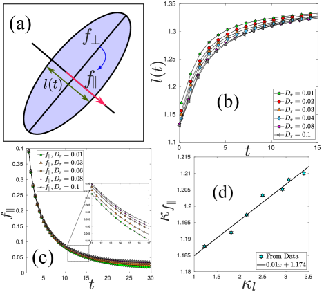
To understand the nature of the force within this elongation time-scale, we have also measured the average forces on the vertices of the cell along the direction of and perpendicular to it, and , respectively. remains nearly the steady state value, but is quite large right after the switch and it then decays over time [Fig. 1(c)]. We define another time-scale, , when decays to half of its initial value. Fig. 1(d) shows that the two time scales, and , are proportional. This establishes that the elongation time-scale is proportional to the time-scale of the active force changes inside the confluent system.
Now consider a scenario where we change the direction of the motile force for a particular cell every time duration, on average. When is much larger compared to , the cell will take a time to elongate along the direction of the active force. Therefore, there will be a delay in the cellular response, to be added to the persistence time of the internal active forces. On the other hand, when is small compared to , the cell cannot follow the rapid change of motile force direction, and the cellular elongation direction will change over a time-scale . Therefore, we can write the effective time-scale for the active force persistence time (and the change of the cell elongation axis) as the sum of these two time-scales
| (4) |
Writing the time-scales in terms of diffusivities, and , we obtain
| (5) |
Since is the effective diffusivity of the active forces (and cell elongations) that give the structural relaxation, in the formalism of extended RFOT theory for self-propulsion Nandi et al. (2018), Eq. (9) below, we must use instead of for a confluent system. As we show below, this modification of due to the constraint of confluency and finite cell elongation time is crucial for the dynamics of confluent systems in the presence of self-propulsion.
We now present our simulation results supporting this physical picture and analytical expression, Eq. (5). To follow the cell elongation direction, characterized by , we first calculate the gyration tensor for each cell and diagonalize it Sadhukhan and Nandi (2022) to obtain two eigenvalues. The eigenvector corresponding to the major eigenvalue, i.e., the major axis direction , gives [Fig. 2(a)]. Note that is nematic by nature as it corresponds to the cell elongation axis. We show in Fig. 2(b) the direction of the internal active force and that of along a trajectory. Fig. 2(c) shows the direction change of the internal active force, , and that of , . Note that the magnitude of is much higher than that of . We obtain from the auto-correlation function of .
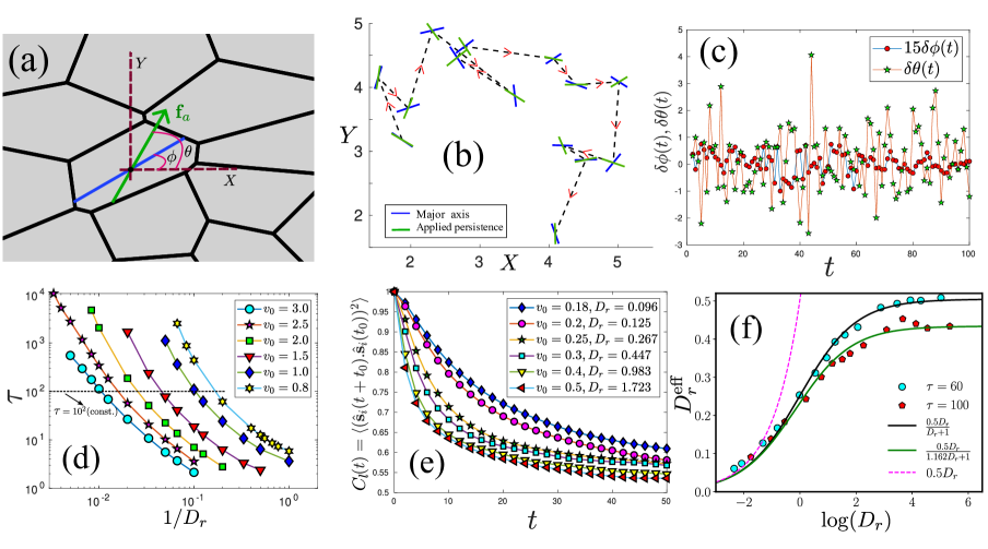
As discussed above, represents a time-scale for cell shape changes, and therefore we expect it to depend on the structural relaxation time of the system (see Appendix E for a mathematical definition). For various and , we have first calculated as a function [Fig. 2(d)]. We then take a line of constant , and for this set of parameters, we calculate the auto-correlation function, , given as
| (6) |
where denotes averages over various cells, initial times , and ensembles Rivas et al. (2020). Note that the definition of in Eq. (6) takes into account the nematic nature of the major axis and . Fig. 2(e) shows the typical behavior of . From these plots, we obtain a time-scale, , by defining a cut-off value of and we obtain . Note that the definition of the cut-off value is arbitrary, and this introduces a scale in . We show the simulation data for as a function of for two different values of in Fig. 2(f). We fit the data with , where accounts for the arbitrary constant introduced by the cut-off value of . We have also used various other cut-off values in our analysis: remains constant for a particular cut-off value. On the other hand, depends on the value of . However, this dependence is not strong: we can ignore the dependence when becomes large. The solid lines in Fig. 2(f) show the comparison of the proposed analytical form [Eq. (5)], and the dashed line shows the behavior when we do not consider the modification due to confluency: the excellent agreement with the simulation data justifies the proposed analytical form. We use for the contribution coming from self-propulsion in the extended RFOT theory below.
III.2 RFOT for the active confluent cell monolayer
The confluent models in the absence of self-propulsion are equilibrium systems. Although in these models actually represents various energy-consuming active processes as well as equilibrium temperature, within the models it has the status of an equilibrium . Such a description agrees well with experiments on systems where self-propulsion is small Park et al. (2015); Atia et al. (2018); Sadhukhan and Nandi (2021); Graner and Glazier (1992); Farhadifar et al. (2007). On the other hand, self-propulsion drives the system out of equilibrium. However, in the regime of small , linear response still applies and we can define a generalized fluctuation-dissipation relation Parisi (2005); Fodor et al. (2016); Sadhukhan and Nandi (2022). We consider a regime where is not very large such that linear response remains applicable. In this regime, the relaxation dynamics remain equilibrium-like at an effective temperature Berthier and Kurchan (2013); Nandi and Gov (2017); Paul et al. (2023). Thus, we treat activity as a small perturbation Nandi et al. (2018); Sadhukhan and Nandi (2021); Paul et al. (2021). The control parameters for the system are and the three parameters of activity: for confluency and and for self-propulsion.
RFOT theory posits that a glassy system consists of mosaics of glassy domains Kirkpatrick and Wolynes (1987); Kirkpatrick et al. (1989); Kirkpatrick and Thirumalai (2015); Lubchenko and Wolynes (2007); Biroli and Bouchaud (2012). The typical length scale of these mosaics comes from a nucleation-like argument. The free energy cost for rearranging a mosaic of length is
| (7) |
where and are the volume and surface area of a unit hypersphere in dimension , is the free energy gain per unit volume, and is the surface free energy cost per unit area. The first term in Eq. (7) gives the free energy gain in the bulk, while the second term gives the cost at its surface due to mismatch. Within RFOT theory, configurational entropy, , is the driving force for the reconfiguration of mosaics and at temperature . Minimizing Eq. (7) yields the domain of length-scale, . We now discuss the effects of self-propulsion and confluency on and .
We first consider the effects of activity on the configurational entropy, , which is governed by the interaction potential and Wolynes and Lubchenko (2012); Parisi and Zamponi (2010); Nandi et al. (2018). We denote the potential energy of the passive system as , and that due to self-propulsion and confluency as and , respectively, and obtain . As discussed above, is a small perturbation in the regime of our interest. The parameter parameterizes . Although is not small for a confluent system, we can still use a perturbative expansion around a reference value.
The constraint of confluency leads to a geometric transition point along . For a polygon of unit area, there is a specific minimum value of the perimeter, , but there is no limit on the maximum value. The ground state of a confluent system consists of hexagons, for which . In the case of disordered systems showing glassy dynamics, becomes slightly higher. has significant role in the static and dynamic properties of confluent systems. When , the system can satisfy the perimeter constraint of Eq. (2), the cells have irregular sides represented by mostly concave polygons, and the system properties do not depend on : this is known as the large- regime Sadhukhan and Nandi (2021). On the other hand, when , the system cannot satisfy the perimeter constraint of Eq. (2), the cells have regular sides (straight or with constant curvature) represented by mostly convex polygons, and the system properties strongly depend on : this is known as the low regime Sadhukhan and Nandi (2021). We take a reference value of , , close to and determine its value via fitting to the simulation data. We take the potential corresponding to as a reference state and treat the potential around this value as a small parameter, i.e., (see Appendix D for an alternative RFOT argument based on this ). Reference Sadhukhan and Nandi (2021) has shown that such a description works well for confluent systems in the absence of self-propulsion. As shown in the Appendix, , and we have
| (8) |
where is the specific heat difference between the liquid and crystalline phase, is the Kauzmann temperature Kauzmann (1948), and are two constants.
Let us now consider the surface term. The temperature dependence of is linear Wolynes and Lubchenko (2012). Therefore, , where the interaction potential also governs the surface energy. For a system of SPPs close to the glass transition, the dominant contribution of self-propulsion comes from the bulk and enters the RFOT theory via Nandi et al. (2018). Assuming to be independent of and provides a good description of the behavior in such systems Nandi et al. (2018). For simplicity, we keep this assumption also for active cell monolayer. On the other hand, confluency results in strong inter-cellular interaction at cell boundaries: this will affect . As detailed in the Appendix A Sadhukhan and Nandi (2021), we have , where and are two constants.
Within RFOT theory, relaxation dynamics occurs via the relaxation of individual mosaics Lubchenko and Wolynes (2007); Biroli and Bouchaud (2012); Nandi et al. (2018). The energy barrier associated with a region of length scale is , where is an energy scale, and is another exponent. Considering a barrier-crossing scenario, we obtain the relaxation time as , where is the relaxation time at high . As detailed in the Appendix A, using Wolynes and Lubchenko (2012); Lubchenko and Wolynes (2007); Biroli and Bouchaud (2012), we obtain
| (9) |
where, , , , and are all constants that we can obtain by fitting the equation with simulation or experimental data. is the effective mean potential energy due to self-propulsion, and we provide its detailed form below. We now confront our theory with new and existing simulation data.
III.3 Comparison with simulation results of active Vertex model
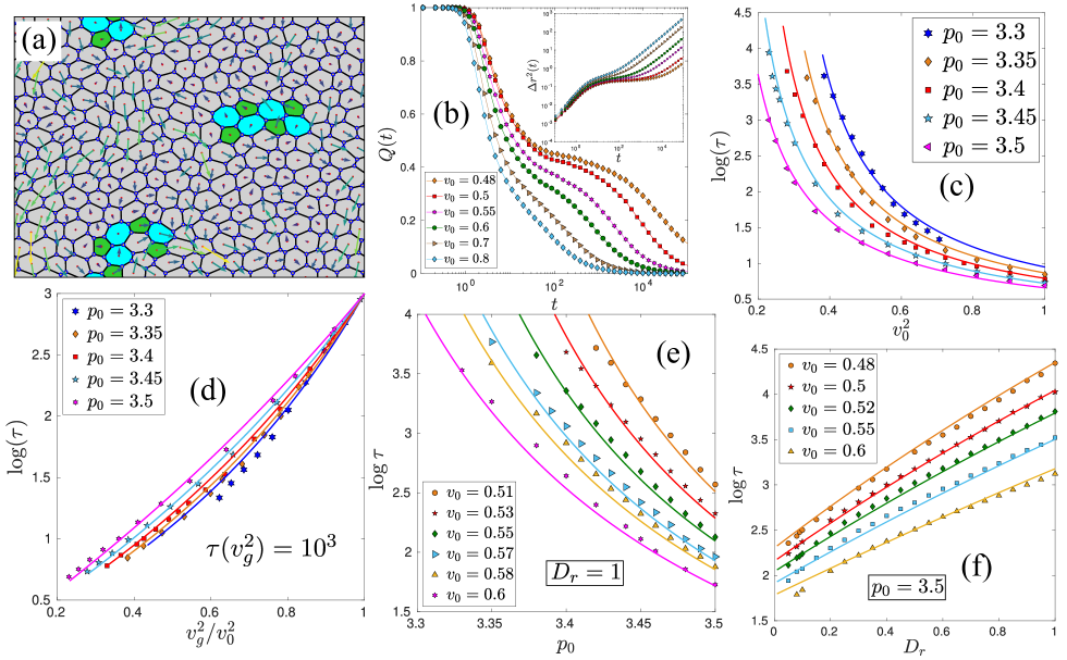
We now compare the theoretical predictions with our simulation results of the active Vertex model (see Appendix E for simulation details). Fig. 3(a) shows a snapshot of the cells with the arrows indicating the self-propulsion direction. To characterize the dynamics, we compute the self-overlap function, , as defined in Appendix E. We show the behavior of for different values of and fixed and in Fig. 3(b). The inset of Fig. 3(b) shows the behavior of the mean-square displacement, (defined in Appendix E). The plateau in and sub-diffusive behavior in are typical of glassy systems Berthier and Biroli (2011); Berthier et al. (2019). We define the relaxation time as . Fig. 3(c) shows the simulation results for (symbols) as a function of for different values of and . To compare with the RFOT theory prediction, we first fix the parameters via fitting Eq. (9) with one set of data. Once these parameters are determined, there exist no other free parameters in the theory and we can then compare the model with the rest of the simulation data. Our simulation results suggest which we have kept constant. As detailed in Ref. Nandi et al. (2018), considering a one-dimensional model for the dynamics of a single self-propelled particle in a confining potential with strength and friction , we obtain
| (10) |
where and . Note that, as discussed in Sec. III.1, we have used [Eq. (5)] instead of in the expression of for a confluent system.
Comparison for varying : Using the expression of in Eq. (9), for fixed and we obtain
| (11) |
where, , , , . Dividing the numerator and denominator of the right-hand side of Eq. (11) by , we obtain
| (12) |
where, , , , and . The simulation results suggest a weak -dependence in . However, for simplicity, we take as a constant. We obtain the rest of the parameters via fit with one particular set of data for : , , , and . There are no other free parameters in the theory and we can compare the theoretical predictions with the simulation data, as shown in Fig. 3(c).
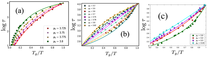
We now present the same data as in Fig. 3(c) in a way that is analogous to the well-known Angell plot Angell (1991, 1995). We define the glass transition point for the self-propulsion velocity, , as . Fig. 3(d) shows as a function of : the lines are the RFOT theory plot, obtained via Eq. (9) with the same parameters used in Fig. 3(c) and the symbols are simulation data. All the curves meet at by definition. The motivation behind plotting the data as a function of instead of is that has the scale of temperature when is constant. In the Angell plot representation, the diagonal line represents the Arrhenius relaxation. All the curves falling below this diagonal line signify super-Arrhenius relaxation.
Comparison for varying : Next, we look at the dynamics as a function of , keeping and fixed. For the comparison with the RFOT theory, we rewrite Eq. (9) as
| (13) |
where, , , and . Note that, in principle, all the parameters, such as , , , and are known. However, since we obtained them via fit, there is always a scope of slight mismatch. To account for this, we use the previously determined values of the first three parameters and treat as a free parameter. We evaluate by fitting to one set of simulation data at . We obtain the value of , which is very close to the previously determined value . We show in Fig. 3(e) that the theoretical predictions (lines) agree very well with the simulation data (symbols) at different values of .
Comparison for varying : We finally study the dynamics at varying , keeping and fixed, and compare it with the RFOT theory. Note that the plateau height in changes with varying . Therefore, to study a range of , we redefine as . The definition does not change any of the physics. This implies that only will change from the previous value. To compare the simulation data from the RFOT theory prediction, we write Eq. (9) as
| (14) |
where we have written the constants in such a way that , , , and remain the same as before and absorbed a constant factor in and . After straightforward algebra, we get,
| (15) |
where, . For comparison with the theory, we now need to determine the constants , , and and (due to the modified definition of ). We obtain these parameters via fits to one dataset, for . With a closer look, we expect (due to the presence of the constant ) and to remain constant. However, and can depend on . We find that their dependence on can be taken as linear: and . We obtain the other two constants as and . With this set of parameters, Fig. 3(f) shows the comparison of simulation data (symbols) with the RFOT theory predictions (lines). Despite all these approximations involved in attaining Eq. (9), the agreement with simulation is remarkable.
III.4 Comparison with existing simulation results
We show that our extended RFOT theory also rationalizes the previously published simulation results on confluent systems. For this purpose, we chose the simulation data for the self-propelled Voronoi model from Bi et al Bi et al. (2016). Specifically, we compare the theory with the simulation results for the fluid-like to solid-like jamming or glass transition phase diagram. In Bi et al. (2016) this transition was defined when the diffusion coefficient, , goes below . However, such a definition is not unique. Since the Stokes-Einstein relation for a suitably chosen gives Pareek et al. (2023), we can equivalently define the glass transition via . We therefore define the glass transition when . As we show below, the functional form governing the phase diagram becomes independent of this specific form of the definition.
We use the expressions for [Eq. (10)] and [Eq. (5)] in Eq. (9), and obtain
| (16) |
To compare the theory with the data of Ref. Bi et al. (2016), we are interested in the phase diagram as functions of , , and at a fixed . Therefore, we can treat as a constant and write
| (17) |
where , and . Now, the definition of the glass transition, , is independent of any control parameter value. Therefore, we can take and and obtain . Therefore, from Eq. (17), we obtain
| (18) |
where . Therefore, the phase boundary governing the solid-like to fluid-like jamming transition is determined by the following equation:
| (19) |
where we have redefined the constants as , , and . The analysis of the data from Ref. Bi et al. (2016) suggests . We obtain the three parameters, , , and , by fitting Eq. (19) with one set of simulation data (Fig. 2(a) of Ref. Bi et al. (2016) for ): , , and . Fig. 4(a) shows the corresponding plot. Once these constants are determined, there are no other free parameters. We can now compare our theory with the other sets of data from Ref. Bi et al. (2016).
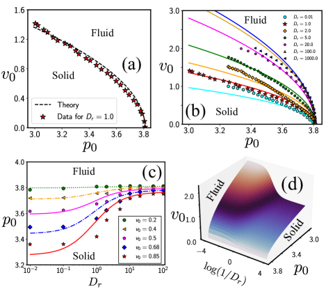
We show in Fig. 4(b) the theoretical predictions (lines) for the solid-like to fluid-like phase boundary in the plane for different values of and also the simulation data by symbols taken from Fig. 3(a) of Ref. Bi et al. (2016). Here, we emphasize two points: first, the theoretical curves are not fits to the simulation data; they are the predictions of the theory given the values of the three constants obtained from the fit in Fig. 4(a). Similar phase diagrams in the plane have been reported in Refs. Barton et al. (2017); Yang et al. (2017) for different realizations of active cell monolayer. Second, such an agreement with the simulation data is impossible without including the effects of confluency on the self-propulsion via Eq. (5). Thus, confluency strongly modifies the effective self-propulsion of the system.
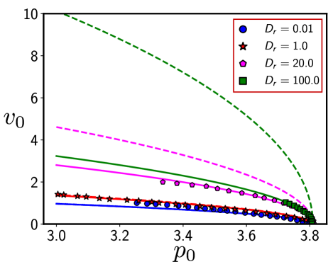
Next, we look at the behavior of the critical value of as a function of for different values of and compare the theory with the simulation data presented in Fig. (3b) of Ref. Bi et al. (2016). We plot our theoretical predictions as lines in Fig. 4(c), and the corresponding simulation data (symbols) are from Ref. Bi et al. (2016). We note here that the values of used in this plot are different from those presented in Ref. Bi et al. (2016). We have chosen such that the theoretical curves match the simulation data. These values of are consistent with the expected values from the other figures in Ref. Bi et al. (2016). The critical value of saturates in both limits when and and agrees well with Eq. (19); in the former case, it saturates to , and in the latter case, it saturates to a value . Summarizing all these results, we can present the solid-like to fluid-like transition in a phase diagram from Eq. (19). We show this phase diagram in Fig. 4(d), and find that it is remarkably similar to the phase diagram of Bi et al. (Fig. 3(c) of Ref. Bi et al. (2016)). Thus, our theory rationalizes the these simulation results.
IV Discussion
To conclude, we have extended the RFOT theory of equilibrium glasses for a confluent system of a cellular monolayer with self-propulsion. We have compared our theoretical predictions with new and existing simulation data, and show that our theory captures the primary characteristics of the glass transition from the solid-like jammed to the fluid-like flowing states in such systems. Understanding the effect of motility on the glassy dynamics of confluent systems is crucial for many biological processes. Our work provides a theoretical framework to understand the nontrivial nature of relaxation dynamics in these systems. Theoretical studies till now have treated the two crucial aspects of biological systems, confluency Sadhukhan and Nandi (2021, 2022), and motility Nandi and Gov (2017); Nandi et al. (2018); Paul et al. (2023); Mandal et al. (2022); Liluashvili et al. (2017); Szamel (2016), separately. Here, for the first time, we have included both aspects within a single theoretical framework and reveal novel features of motility-driven glassy dynamics in confluent epithelial systems.
The crucial result of this work is that confluency modifies the effective persistence time of self-propulsion. This modification appears as an effective rotational diffusivity, of the active propulsion forces. In cellular systems, a cell needs time to elongate along the changing direction of the active force, and this elongation time, , should depend on both (or ) and of the system. We have shown in our simulations that relates the time scale of active force relaxation as well as that of the cellular elongation. Using , we have phenomenologically obtained an analytical expression for the modified diffusivity of the active force and verified it in our simulation.
Analysis of the relaxation dynamics of existing and new simulation results seem to suggest that is crucial for confluent cellular systems. We have shown in Fig. 6 that one cannot explain the simulation results for the relaxation dynamics without considering . In the experimental context, one can vary the cellular activity through different oncogenes, such as the Ras Gysin et al. (2011), or via growth factors, such as the protein kinase C Rodrigues et al. (2019). For example, a tumor suppressor protein, Merlin, increases directional persistence and reduces motility force in Madin–Darby canine kidney (MDCK) dog epithelial cells das2015. However, the change in the dynamics should be less sensitive to the change in at when persistence is high due to the effect of confluency where becomes nearly constant when is large.
Within the theoretical descriptions of confluent systems via Eq. (2), parameterizes inter-cellular interaction. The phase diagrams in Fig. 4 suggest that the system remains fluid beyond a specific value of . The parameter in Eq. (19) is crucial in obtaining this behavior. Our theory does not predict ; it is an input. We provide an alternate argument in Appendix D for the extended RFOT theory for confluent systems based on . The value of seems to vary for different systems and depends on the details of the models. It is possibly related to the geometric constraint leading to . seems to control the glassy dynamics in confluent systems, and it is critical to understand what leads to and how it affects the dynamical behavior.
The glassy behavior with changing self-propulsion velocity, , seems similar to that in particulate systems where increasing fluidizes the system. However, the behavior with varying seems non-trivial, where the plateau height in seems to vary. This behavior generally signifies a variation in caging length. We will explore this aspect in more detail later. The other aspect, specific to confluent systems, is the fluidization with increasing even when is much lower than . As shown in Fig. 3(e), decreases with increasing . Experiments seem to agree with this result Garcia et al. (2015); Bazellières et al. (2015). For example, Ref. Malinverno et al. (2017) have shown that expression of RAB5A, a key endocytic protein, produces large-scale motion and fluidizes a solid-like jammed tissue of human mammary epithelial MCF-10A cells. RAB5A enhances endosomal trafficking and macropinocytic internalization and, thus, facilitates the dynamics of cellular junctional proteins, reducing inter-cellular interaction. This effect implies an increase in that leads to fluidization, much like the results of Fig. 3(e).
Apart from their biological significance, the glassy dynamics in confluent systems is interesting from the perspective of theories of glassy systems. The confluent systems provide a rich testing ground for various theories of glassy dynamics. They can be viewed as limiting systems for the highly dense aggregates of soft particles. The glassy dynamics in dense systems of soft particles show several intriguing properties, such as super-diffusive behavior Gnan and Zaccarelli (2019) or sub-Arrhenius relaxation Berthier and Witten (2009a, b); Adhikari et al. (2022). Such behaviors are abundant in confluent systems Park et al. (2015); Sussman et al. (2018); Sadhukhan and Nandi (2021). Specifically, the sub-Arrhenius relaxation in these systems seems to result in a negative implying a finite relaxation time even at zero . Based on this result, we can define a and develop the RFOT arguments as in Appendix D. These arguments show that the relaxation should become super-Arrhenius at lower values of Sadhukhan and Nandi (2021). We have verified this prediction for the cellular Potts model in Ref. Sadhukhan and Nandi (2021) and for the Voronoi and the Vertex models here (Appendix B). In our simulation, we have chosen the parameters such that we are in the super-Arrhenius regime (Fig. 3). On the other hand, the sub-Arrhenius regime seems to be nearly ideal for the mode-coupling theory of glassy dynamics Pandey et al. (2023). How the same system crosses over from one mechanism to the other for the relaxation dynamics and if it is similar in equilibrium systems remain fascinating questions.
Finally, our work provides a foundation for a deeper understanding of the fascinating glassy aspects of confluent systems, both from biological and theoretical perspectives. There are many critical questions in this direction. It is well-known that cell shape is closely related to dynamics in confluent systems Atia et al. (2018); Sadhukhan and Nandi (2022); Arora et al. (2024). It will be intriguing to include metrics of cell shape within the RFOT theory framework to study how the dynamics and statics are connected. Moreover, cellular shapes are also related to functions. Such a framework will allow us to analyze shape, dynamics, and function within a single framework. Besides, perturbing one particular protein in a biological system can have multiple effects. A detailed understanding of how various parameters affect the dynamic behavior can reveal the actual consequences of such perturbations in experiments and eventually allow us to design diverse gene-level manipulations to target specific aspects of the system.
We have shown that the extended RFOT theory captures several glassy aspects in confluent models of epithelial systems. The main ingredients of the theory are (1) the mosaic-like nature whose length-scale comes from the competition of surface and bulk free energies leading to a nucleation-like scenario, (2) the geometric constraint leading to a reference state, given by , and (3) the modified of the active force, due to its coupling with cell elongation, that allows structural relaxation. Using new and existing simulation data, we have tested the predictions against two distinct models of confluent systems, the Vertex model (Fig. 3) and the Voronoi model (Fig. 4). Therefore, we believe the theory should be applicable in general, including particle-based models of confluent monolayers Tarle et al. (2015); Sarkar et al. (2021).
Acknowledgments
We thank Daniel Sussman for sharing the data of for bidisperse Voronoi model from Ref. Sussman et al. (2018). SS thanks “Infosys-TIFR Leading Edge Travel Grant”, Ref.No.: TFR/Efund/44/Leading Edge TG(R-3)/09/ for the funding for travel to Israel. MP acknowledges NextGeneration EU (CUP B63C22000730005) within the Project IR0000029 - Humanities and Cultural Heritage Italian Open Science Cloud (H2IOSC) - M4, C2, Action 3.1.1. We acknowledge the support of the Department of Atomic Energy, Government of India, under Project Identification No. RTI 4007. S.K.N. thanks SERB for grant via SRG/2021/002014.
Appendix A Details of the RFOT theory calculation
As discussed in the main text, both the configurational entropy, , and the surface energy are functions of the interaction potential of the system Parisi and Zamponi (2010); Nandi et al. (2018). For our system, we write the total interaction potential as sum of three distinct contributions: for the passive system, for the self-propulsion, and for confluency. Thus, and . We assume that self-propulsion, and hence , is low and a generalized fluctuation-dissipation relation is valid. For a confluent system, itself cannot be small as the system remains confluent at all times. The interaction potential is parameterized by . We assume a reference state given by and the corresponding value of potential as . Thus, , where is small. Therefore, we have
| (20) |
where is the configurational entropy of the reference system, and are constants. We assume the reference system follows the RFOT theory: the configurational entropy vanishes at the Kauzmann temperature . Therefore, we can write close to as , where is the difference in specific heat between the liquid and the periodic crystalline phase Kauzmann (1948).
The interaction energy in confluent systems is given by the perimeter term, and we can write Sadhukhan and Nandi (2021) . Therefore, we have , where is a constant. Then, we can write as
| (21) |
where is another constant. On the other hand, following Ref. Nandi et al. (2018), we ignore the contribution of to the surface reconfiguration energy, thus . Expanding the effect of confluency around the reference state, we obtain
| (22) |
Using similar arguments as above, we can write .
As shown in the main text, the typical length scale of the mosaics is
| (23) |
Relaxation within RFOT theory is described by the relaxation of the individual mosaics. Considering a barrier-crossing scenario, we have the relaxation time
| (24) |
where is an energy scale and is the high relaxation time. Substituting the value of above, we get
| (25) |
Using the expressions of and , and Wolynes and Lubchenko (2012); Lubchenko and Wolynes (2007); Biroli and Bouchaud (2012), we obtain,
| (26) |
where, , , and .
Appendix B The RFOT theory prediction of super- and sub-Arrhenius regimes in confluent systems
One unusual aspect of the glassy dynamics in confluent systems is the readily found sub-Arrhenius relaxation dynamics: In the Angell plot representation Angell (1991, 1995), plotting as a function of , where is the glass transition temperature, a straight line represents the Arrhenius relaxation, that is grows as an exponential of . When relaxation is super-Arrhenius, i.e., faster than exponential, the curve appears below the straight line. In contrast, when relaxation is sub-Arrhenius, i.e., slower than exponential, it appears above the straight line. All the models of confluent systems, the Vertex model, the Voronoi model Sussman et al. (2018), and the CPM Sadhukhan and Nandi (2021) show sub-Arrhenius behavior for certain values of the parameters. The extended RFOT theory for the glassy dynamics in confluent systems Sadhukhan and Nandi (2021) predicts that , the effective Kauzmann temperature, becomes negative in the sub-Arrhenius regime. This result suggests that does not diverge even at zero . On the other hand, Ref. Pandey et al. (2023) showed that another theory, the mode-coupling theory (MCT), applies remarkably well in this regime and diverges at a finite as a power law.
On the other hand, the extended RFOT theory also predicts the presence of super-Arrhenius relaxation at lower values Sadhukhan and Nandi (2021). This prediction has been tested for the CPM Sadhukhan and Nandi (2021) and the Voronoi model Li et al. (2021). In the main text, we have shown that the super-Arrhenius regime exists in the self-propelled Vertex model. Here we show that this specific prediction is also valid for the equilibrium Vertex model and provide detailed comparison of the RFOT theory for the equilibrium Voronoi and Vertex models..
For the passive systems, the RFOT expression, Eq. (9), becomes
| (27) |
where and . We first compare the theory with the existing Voronoi model simulation data presented in Ref. Sussman et al. (2018). We find that gives a good description of the simulation data, and fitting Eq. (27) with one set of data, we find , , , and . Fig. 5(a) shows the comparison of the theory (lines) with the simulation data of Ref. Sussman et al. (2018) (symbols). Using these values of the constants, it is easy to verify that becomes negative for these set of curves in Fig. 5. This is consistent with the fact that the curves represent sub-Arrhenius behaviors.
According to the RFOT theory, we expect the behavior to become super-Arrhenius at lower , however, Sussman et al did not explore this regime Sussman et al. (2018). Since the detailed values of the parameters depend on the specific system, to test this aspect, we first present simulation data for the equilibrium Voronoi model for a range of values showing both the super- and sub-Arrhenius behavior. For our system with , , and , we find , , , , and . We show the comparison of our simulation data with Eq. (27) in Fig. 5(b). Consistent with the results of Ref. Sussman et al. (2018), the relaxation dynamics is sub-Arrhenius for the range of , and then the dynamics becomes super-Arrhenius for lower , as also found in Ref. Li et al. (2021).
We finally present our simulation results for the equilibrium Vertex model testing the prediction for the super-Arrhenius behavior at lower values. For these simulations, we have used the open-source software RheoVM Tong et al. (2022) to simulate the Vertex model via Brownian dynamics. We have used a system size of with cells, preferred area , , and . We take the friction coefficient for the Brownian dynamics as . For the clarity of presentation, we only show the super-Arrhenius behavior for the lower values of in Fig. 5(c). Our analysis suggests the value of . Fitting one set of data gives the values of the constants in Eq. 27 as follows: , ; , and . Fig. 5(c) shows the simulation data via symbols and the corresponding RFOT theory plot of Eq. (27) by lines; the theory agrees remarkably well in this regime with the simulation data.
Appendix C Confluency modification of
We stated in the main text, Sec. III.1, that the confluency modifies the rotational diffusivity of self-propulsion and leads to [Eq. (5)]. enters the RFOT theory, and we have shown the comparison with simulation data in Figs. 3 and 4 in the main text. We show in Fig. 6 that this modification is crucial for agreement with the simulation data. We present the phase diagrams at various with this modification and without it (that is, in Eq. (5)), by solid and dashed lines, respectively. Since is very close to , they nearly agree with each other for and . However, they deviate strongly for the higher values of .
Appendix D An alternative argument for the RFOT theory of confluent systems
We have argued, via existing and new simulation results, that the dynamics in confluent systems is sub-Arrhenius at larger values of , and it becomes super-Arrhenius as decreases. Furthermore, the application of the RFOT theory to the sub-Arrhenius regime leads to a negative effective Kauzmann temperature, . However, is positive in the super-Arrhenius regime, and the usual arguments of RFOT theory applies Biroli and Bouchaud (2012). Based on this observation, we can develop a RFOT argument to extend the theory for such systems to understand the effect of . Since this argument is specific to the confluent systems, for simplicity, we present it for equilibrium systems alone. The self-propulsion can be included in a similar way as discussed in the main text.
Within RFOT theory, the mosaic length is determined by the competition of an energy cost at the surface and gain in the bulk. The latter is governed by the configurational entropy, , which determines the critical behavior. For the confluent systems, . We assume that for ,
| (28) |
where is a -dependent constant. here also depends on and we will obtain this dependence below. gives the regime below which the theory is applicable. The simulation results show that should be taken as , where the dynamics is Arrhenius-like. Thus, the theory should be applicable for values of below . We assume that is a smooth function of when is close to , therefore, we can write
| (29) |
where is a positive constant. Thus, we have
Using this expression for along with the arguments presented in Sec. III.2, we obtain the RFOT theory for the confluent system in the absence of self-propulsion as
| (30) |
Note that this result is valid for . The system will have dynamics in this regime, and the dynamics freezes in the other regime.
Appendix E Simulation details for the Vertex model
Here we provide additional details for the self-propelled Vertex Model (VM). To include self-propulsion, we associate each cell with a self-propulsion force of magnitude (or velocity considering ). acts along a polarity vector, , where is an angle measured from the -axis. The total self-propulsion force on each vertex (), , is the mean self-propulsion forces of the 3 cells that share vertex . We assume over-damped dynamics and write the equation of motion of vertex as
| (31) |
where is the force arising from the mechanical energy, Eq. (2), of the tissue. is the random thermal noise with mean zero and standard deviation, , with being the unit tensor; we have set to unity. is the active force acting on vertex : , where is the list of neighboring cells sharing vertex . performs a rotational Brownian motion [Eq. (3)]. We have used the Euler-Murayama integration scheme to update the discretized version of the equations (for each vertex).
To highlight the effects of activity, we have used in our simulations. Other parameters are as follows; , , , , , , , . Our unit of length is and unit of time is . Unless otherwise specified, we have equilibrated the system for times before collecting the data, performed averaging and ensemble averaging, and simulated cells.
Self-overlap function, : In our simulations, we compute the center of mass, , for the cells from the positions of their vertices. We then define the self-overlap function, , as
| (32) |
where is the Heaviside step function:
| (33) |
The parameter is set to a constant value of throughout the simulation. This value of corresponds to the caging length scale of vibrational motions revealed via the MSD [inset of Fig. 3(b)]. The angular brackets denote initial time and ensemble averages. We define the structural relaxation time as .
Mean-square displacement, : We define as
| (34) |
References
- Tambe et al. (2011) D. T. Tambe, C. C. Hardin, T. E. Angelini, K. Rajendran, C. Y. Park, X. Serra-Picamal, E. H. Zhou, M. H. Zaman, J. P. Butler, D. A. Weitz, J. J. Fredberg, and X. Trepat, Nat. Mater. 10, 469 (2011).
- Friedl and Gilmour (2009) P. Friedl and D. Gilmour, Nat. Rev. Mol. Cell Biol. 10, 445 (2009).
- Malmi-Kakkada et al. (2018) A. N. Malmi-Kakkada, X. Li, H. S. Samanta, S. Sinha, and D. Thirumalai, Phys. Rev. X 8, 021025 (2018).
- Schötz et al. (2013) E.-M. Schötz, M. Lanio, J. A. Talbot, and M. L. Manning, J. R. Soc. Interface 10, 20130726 (2013).
- Poujade et al. (2007) M. Poujade, E. Grasland-Mongrain, A. Hertzog, J. Jouanneau, P. Chavrier, B. Ladoux, A. Buguin, and P. Silberzan, Proc. Natl. Acad. Sci. (USA) 104, 15988 (2007).
- Das et al. (2015) T. Das, K. Safferling, S. Rausch, N. Grabe, H. Boehm, and J. P. Spatz, Nat. Cell Biol. 17, 276 (2015).
- Brugués et al. (2014) A. Brugués, E. Anon, V. Conte, J. H. Veldhuis, M. Gupta, J. Colombelli, J. J. Muñoz, G. W. Brodland, B. Ladoux, and X. Trepat, Nat. Phys. 10, 683 (2014).
- Malinverno et al. (2017) C. Malinverno, S. Corallino, F. Giavazzi, M. Bergert, Q. Li, M. Leoni, A. Disanza, E. Frittoli, A. Oldani, E. Martini, T. Lendenmann, G. Deflorian, G. V. Beznoussenko, D. Poulikakos, K. H. Ong, M. Uroz, X. Trepat, D. Parazzoli, P. Maiuri, W. Yu, A. Ferrari, R. Cerbino, and G. Scita, Nat. Mater. 16, 587 (2017).
- Streitberger et al. (2020) K.-J. Streitberger, L. Lilaj, F. Schrank, a. K.-T. H. Jürgen Braun, M. Reiss-Zimmermann, J. A. Käs, and I. Sack, Proc. Natl. Acad. Sci. (USA) 117, 128 (2020).
- Friedl and Wolf (2003) P. Friedl and K. Wolf, Nat. Rev. Cancer 3, 362 (2003).
- Berthier and Biroli (2011) L. Berthier and G. Biroli, Rev. Mod. Phys. 83, 587 (2011).
- Pareek et al. (2023) P. Pareek, M. Adhikari, C. Dasgupta, and S. K. Nandi, J. Chem. Phys. 159, 174503 (2023).
- Angelini et al. (2011) T. E. Angelini, E. Hannezo, X. Trepat, M. Marquez, J. J. Fredberg, and D. A. Weitz, Proc. Natl. Acad. Sci. (USA) 108, 4717 (2011).
- Park et al. (2015) J.-A. Park, J. H. Kim, D. Bi, J. A. Mitchel, N. T. Qazvini, K. Tantisira, C. Y. Park, M. McGill, S.-H. Kim, B. Gweon, J. Notbohm, R. S. Jr, S. Burger, S. H. Randell, A. T. Kho, D. T. Tambe, C. Hardin, S. A. Shore, E. Israel, D. A. Weitz, D. J. Tschumperlin, E. P. Henske, S. T. Weiss, M. L. Manning, J. P. Butler, J. M. Drazen, and J. J. Fredberg, Nat. Mater. 14, 1040 (2015).
- Nnetu et al. (2012) K. D. Nnetu, M. Knorr, D. Strehle, M. Zink, and J. A. Käs, Soft Matter 8, 6913 (2012).
- Szabó et al. (2006) B. Szabó, G. J. Szöllösi, B. Gönci, Z. Jurányi, D. Selmeczi, and T. Vicsek, Phys. Rev. E 74, 061908 (2006).
- Trepat et al. (2009) X. Trepat, M. R. Wasserman, T. E. Angelini, E. Millet, D. A. Weitz, J. P. Butler, and J. J. Fredberg, Nat. Phys. 5, 426 (2009).
- Giavazzi et al. (2018) F. Giavazzi, C. Malinverno, G. Scita, and R. Cerbino, Front. Phys. 6, 120 (2018).
- Atia et al. (2021) L. Atia, J. J. Fredberg, N. S. Gov, and A. F. Pegoraro, Cells and Development 168, 203727 (2021).
- Paul et al. (2021) K. Paul, S. K. Nandi, and S. Karmakar, arXiv , 2111.09829 (2021).
- Paul et al. (2023) K. Paul, A. Mutneja, S. K. Nandi, and S. Karmakar, Proc. Natl. Acad. Sci. (USA) 120, e2217073120 (2023).
- Prost et al. (2015) J. Prost, F. Jülicher, and J. F. Joanny, Nat. Phys. 11, 111 (2015).
- Ranft et al. (2010) J. Ranft, M. Basan, J. Elgeti, J.-F. Joanny, J. Prost, and F. Jülicher, Proc. Natl. Acad. Sci. (USA) 107, 20863 (2010).
- Matoz-Fernandez et al. (2017) D. A. Matoz-Fernandez, K. Martens, R. Sknepnek, J. L. Barrat, and S. Henkes, Soft Matter 13, 3205 (2017).
- Alvarado and Yamanaka (2014) A. S. Alvarado and S. Yamanaka, Cell 157, 110 (2014).
- Farhadifar et al. (2007) R. Farhadifar, J.-C. Röper, B. Aigouy, S. Eaton, and F. Jülicher, Curr. Biol. 17, 2095 (2007).
- Garcia et al. (2015) S. Garcia, E. Hannezo, J. Elgeti, J. F. Joanny, P. Silberzan, and N. S. Gov, Proc. Natl. Acad. Sci. (USA) 112, 15314 (2015).
- Ramaswamy (2010) S. Ramaswamy, Annu. Rev. Condens. Matter Phys. 1, 323 (2010).
- Marchetti et al. (2013) M. C. Marchetti, J. F. Joanny, S. Ramaswamy, T. B. Liverpool, J. Prost, M. Rao, and R. A. Simha, Rev. Mod. Phys. 85, 1143 (2013).
- Janssen (2019) L. M. C. Janssen, J. Phys.: Condens. Matter 31, 503002 (2019).
- Berthier et al. (2019) L. Berthier, E. Flenner, and G. Szamel, J. Chem. Phys. 150, 200901 (2019).
- Paoluzzi et al. (2022) M. Paoluzzi, D. Levis, and I. Pagonabarraga, Commun Phys 5, 111 (2022).
- Palacci et al. (2010) J. Palacci, C. Cottin-Bizonne, C. Ybert, and L. Bocquet, Phys. Rev. Lett. 105, 088304 (2010).
- Szamel (2014) G. Szamel, Phys. Rev. E 90, 012111 (2014).
- Han et al. (2017) M. Han, J. Yan, S. Granick, and E. Luijten, Proc. Natl. Acad. Sci. (USA) 114, 7513 (2017).
- Fodor et al. (2016) E. Fodor, C. Nardini, M. E. Cates, J. Tailleur, P. Visco, and F. van Wijland, Phys. Rev. Lett. 117, 038103 (2016).
- Parisi (2005) G. Parisi, Nature 433, 221 (2005).
- Berthier (2014) L. Berthier, Phys. Rev. Lett. 112, 220602 (2014).
- Mandal et al. (2016) R. Mandal, P. J. Bhuyan, M. Rao, and C. Dasgupta, Soft Matter 12, 6268 (2016).
- Flenner et al. (2016) E. Flenner, G. Szamel, and L. Berthier, Soft Matter 12, 7136 (2016).
- Ni et al. (2013) R. Ni, M. A. C. Stuart, and M. Dijkstra, Nat. Commun 4, 2704 (2013).
- Klongvessa et al. (2019a) N. Klongvessa, F. Ginot, C. Ybert, C. Cottin-Bizonne, and M. Leocmach, Phys. Rev. Lett. 123, 248004 (2019a).
- Klongvessa et al. (2019b) N. Klongvessa, F. Ginot, C. Ybert, C. Cottin-Bizonne, and M. Leocmach, Phys. Rev. E 100, 062603 (2019b).
- Arora et al. (2022) P. Arora, A. K. Sood, and R. Ganapathy, Phys. Rev. Lett. 128, 178002 (2022).
- Berthier and Kurchan (2013) L. Berthier and J. Kurchan, Nat. Phys. 9, 310 (2013).
- Szamel (2016) G. Szamel, Phys. Rev. E 93, 012603 (2016).
- Liluashvili et al. (2017) A. Liluashvili, J. Ónody, and T. Voigtmann, Phys. Rev. E 96, 062608 (2017).
- Feng and Hou (2017) M. Feng and Z. Hou, Soft Matter 13, 4464 (2017).
- Nandi and Gov (2017) S. K. Nandi and N. S. Gov, Soft Matter 13, 7609 (2017).
- Nandi et al. (2018) S. K. Nandi, R. Mandal, P. J. Bhuyan, C. Dasgupta, M. Rao, and N. S. Gov, Proc. Natl. Acad. Sci. (USA) 115, 7688 (2018).
- Mandal et al. (2022) R. Mandal, S. K. Nandi, C. Dasgupta, P. Sollich, and N. S. Gov, J. phys. commun. 6, 115001 (2022).
- Graner and Glazier (1992) F. Graner and J. A. Glazier, Phys. Rev. Lett. 69, 2013 (1992).
- Glazier and Graner (1993) J. A. Glazier and F. Graner, Phys. Rev. E 47, 2128 (1993).
- Hogeweg (2000) P. Hogeweg, J. Theor. Biol. 203, 317 (2000).
- Hirashima et al. (2017) T. Hirashima, E. G. Rens, and R. M. H. Merks, Develop. Growth Differ. 59, 329 (2017).
- Chiang and Marenduzzo (2016) M. Chiang and D. Marenduzzo, EPL (Europhysics Letters) 116, 28009 (2016).
- Sadhukhan and Nandi (2021) S. Sadhukhan and S. K. Nandi, Phys. Rev. E 103, 062403 (2021).
- Honda and Eguchi (1980) H. Honda and G. Eguchi, J. Theor. Biol. 84, 575 (1980).
- Marder (1987) M. Marder, Phys. Rev. A 36, 438(R) (1987).
- Fletcher et al. (2014) A. G. Fletcher, M. Osterfield, R. E. Baker, and S. Y. Shvartsman, Biophys. J. 106, 2291 (2014).
- Bi et al. (2016) D. Bi, X. Yang, M. C. Marchetti, and M. L. Manning, Phys. Rev. X 6, 021011 (2016).
- Li et al. (2021) Y.-W. Li, L. L. Y. Wei, M. Paoluzzi, and M. P. Ciamarra, Phys. Rev. E 103, 022607 (2021).
- Czajkowski et al. (2019) M. Czajkowski, D. M. Sussman, M. C. Marchetti, and M. L. Manning, Soft Matter 15, 9133 (2019).
- Nonomura (2012) M. Nonomura, PLoS ONE 7, e33501 (2012).
- Palmieri et al. (2015) B. Palmieri, Y. Bresler, D. Wirtz, and M. Grant, Sci. Rep. 5, 11745 (2015).
- Loewe et al. (2020) B. Loewe, M. Chiang, D. Marenduzzo, and M. C. Marchetti, Phys. Rev. Lett. 125, 038003 (2020).
- Bi et al. (2014) D. Bi, J. H. Lopez, J. M. Schwarz, and M. L. Manning, Soft Matter 10, 1885 (2014).
- Sussman et al. (2018) D. M. Sussman, M. Paoluzzi, M. C. Marchetti, and M. L. Manning, Europhys. Lett. 121, 36001 (2018).
- Sadhukhan and Nandi (2022) S. Sadhukhan and S. K. Nandi, eLife 11, e76406 (2022).
- Lubchenko and Wolynes (2007) V. Lubchenko and P. G. Wolynes, Annu. Rev. Phys. Chem. 58, 235 (2007).
- Kirkpatrick and Thirumalai (2015) T. R. Kirkpatrick and D. Thirumalai, Rev. Mod. Phys. 87, 183 (2015).
- Biroli and Bouchaud (2012) G. Biroli and J. P. Bouchaud, in Structural Glasses and Supercooled Liquids: Theory, Experiment, and Applications, edited by P. G. Wolynes and V. Lubchenko (2012).
- Weaire and Hutzler (2001) D. Weaire and S. Hutzler, Thephysicsof foams (Oxford University Press, 2001).
- Albert and Schwarz (2016) P. J. Albert and U. S. Schwarz, Cell Adhesion & Migration 10, 516 (2016), pMID: 26838278.
- Barton et al. (2017) D. L. Barton, S. Henkes, C. J. Weijer, and R. Sknepnek, Plos Comput. Biol. 13, e1005569 (2017).
- Yang et al. (2017) X. Yang, D. Bi, M. Czajkowski, M. Merkel, M. L. Manning, and M. C. Marchetti, Proc. Natl. Acad. Sci. (USA) 114, 12663 (2017).
- Wolff et al. (2019) H. B. Wolff, L. A. Davidson, and R. M. H. Merks, Bul. Math. Biol. 81, 3322 (2019).
- Paoluzzi et al. (2021) M. Paoluzzi, L. Angelani, G. Gosti, M. C. Marchetti, I. Pagonabarraga, and G. Ruocco, Phys. Rev. E 104, 044606 (2021).
- Rivas et al. (2020) D. P. Rivas, T. N. Shendruk, R. R. Henry, D. H. Reich, and R. L. Leheny, Soft Matter 16, 9331 (2020).
- Atia et al. (2018) L. Atia, D. Bi, Y. Sharma, J. A. Mitchel, B. Gweon, S. A. Koehler, S. J. DeCamp, B. Lan, J. H. Kim, R. Hirsch, A. F. Pegoraro, K. H. Lee, J. R. Starr, D. A. Weitz, A. C. Martin, J.-A. Park, J. P. Butler, and J. J. Fredberg, Nat. Phys. 14, 613 (2018).
- Kirkpatrick and Wolynes (1987) T. R. Kirkpatrick and P. G. Wolynes, Phys. Rev. A 35, 3072 (1987).
- Kirkpatrick et al. (1989) T. R. Kirkpatrick, D. Thirumalai, and P. G. Wolynes, Phys. Rev. A 40, 1045 (1989).
- Wolynes and Lubchenko (2012) P. G. Wolynes and V. Lubchenko, Structural Glasses and Supercooled Liquids (John Wiley and Sons, Inc., Hoboken, New Jersey, 2012).
- Parisi and Zamponi (2010) G. Parisi and F. Zamponi, Rev. Mod. Phys. 82, 789 (2010).
- Kauzmann (1948) W. Kauzmann, Chemical Reviews 43, 219 (1948).
- Angell (1991) C. A. Angell, J. Non-Cryst. Solids 131-133, 13 (1991).
- Angell (1995) C. A. Angell, Science 267, 1924 (1995).
- Gysin et al. (2011) S. Gysin, M. Salt, A. Young, and F. McCormick, Genes and Cancer 2, 359 (2011).
- Rodrigues et al. (2019) M. Rodrigues, N. Kosaric, C. A. Bonham, and G. C. Gurtner, Physiol. Rev. 99, 665 (2019).
- Bazellières et al. (2015) E. Bazellières, V. Conte, A. Elosegui-Artola, X. Serra-Picamal, M. Bintanel-Morcillo, P. Roca-Cusachs, J. J. Muñoz, M. Sales-Pardo, R. Guimerà, and X. Trepat, Nat. Cell Biol. 17, 409 (2015).
- Gnan and Zaccarelli (2019) N. Gnan and E. Zaccarelli, Nat. Phys. 15, 683 (2019).
- Berthier and Witten (2009a) L. Berthier and T. A. Witten, Phys. Rev. E 80, 021502 (2009a).
- Berthier and Witten (2009b) L. Berthier and T. A. Witten, Europhys. Lett. 86, 10001 (2009b).
- Adhikari et al. (2022) M. Adhikari, S. Karmakar, and S. Sastry, arXiv , 2204.02936 (2022).
- Pandey et al. (2023) S. Pandey, S. Kolya, S. Sadhukhan, and S. K. Nandi, arXiv v1, 2306.07250 (2023).
- Arora et al. (2024) P. Arora, S. Sadhukhan, S. K. Nandi, D. Bi, A. K. Sood, and R. Ganapathy, arXiv , 2401.13437 (2024).
- Tarle et al. (2015) V. Tarle, A. Ravasio, V. Hakim, and N. S. Gov, Int. Biol. 7, 1218 (2015).
- Sarkar et al. (2021) D. Sarkar, G. Gompper, and J. Elgeti, Comm. Phys. 4, 36 (2021).
- Tong et al. (2022) S. Tong, N. K. Singh, R. Sknepnek, and A. Košmrlj, PLOS Comput. Biol. 18, 1 (2022).