Observational tests in scale invariance II: gravitational lensing

Abstract

We study the path of light rays passing near a massive object, in the context of the scale invariant equation of the geodesics first obtained by Dirac (1973). Using the exterior Schwarzschild solution for the metric, we derive the complete equations of the geodesics in the scale invariant context. We find that scale invariance introduces two additional terms to the Einstein term producing the deflection angle and that can potentially act over cosmological distances. Numerical integration of the scale-invariant geodesics, for the specific case of the $z_{L}=1.94$ lens galaxy in the extreme system JWST-ER1 (van Dokkum et al. 2023) shows that the two additional terms introduce only negligible effects, typically $\mathcal{O}$($10^{-6}$) of the Einstein term. We conclude that the lensing deflection angle derived in Einstein’s General Relativity is essentially independent of the scale invariant effects and that the photon’s geodesics remain unchanged. We also explore the possible origin of the differences in the mass estimates from lensing and photometry in JWST-ER1 and in the SLACS galaxies, differences which appear larger at higher redshifts.

1 Introduction

Gravitational lensing is a powerful natural phenomenon featuring a vast range of astrophysical and cosmological applications. Its major strength is that it gives access to quantities that are notoriously hard to measure otherwise, masses and mass distributions at all spatial scales being the main ones. Gravitational lensing is also one of the key observations that confirmed General Relativity (GR), through the measurement of the light deflection angle by the Sun during the 1919 Solar eclipse [10]. It therefore consists in a perfect laboratory to test alternative scenario to $\Lambda$CDM, such as scale invariant theory [19, 21, 26].

This is particularly useful in light of recent observational tests of scale invariant theory, (see paper I [22]). It explains: - why the standard mass estimates from galaxy velocities are overestimating the mass of galaxy clusters, - flat rotation curves of galaxies [20], - why the observed projected velocities of wide binary stars are overestimated by standard theory as their angular separation increases [13]. Other effects are mentioned in Paper I.

In the present work, we confront scale invariant theory to strong gravitation lensing observations at galaxy scale. We compute the geodesic equations in the scale invariance context and show that they do not differ from the standard GR derivation. While scale invariance has no effect on the photons’ geodesics themselves, we show that it has an effect on the interpretation and use of the mass-luminosity relation of the stellar population in the lens galaxy and of its IMF. We illustrate this with real observations of strongly lensed galaxies, focusing on the extreme case of the ”dark lens” JWST-ER1 [38] at $z_{L}=1.94$ and on the text-book SLACS sample of lenses at $z_{L}$between 0 and 0.5 for which excellent spectroscopic observations are available [1]. This allows us to confront the standard lensing masses at very different redshifts to the luminous masses in the scale invariant framework.

In Section 2 we give a brief summary of the scale invariant theory. Section 3 describes the calculation of trajectories of lensed light paths in the scale invariant context. Section 4 shows from accurate numerical integration that scale invariant effects on the light rays are negligible. Section 5 examines the origin of the discrepancy between the stellar masses and the masses from the lensing and exposes the scale invariant effects that reconcile the two mass estimates. These are further discussed in Section 6 which also proposes additional future tests involving gravitational lensing. Finally, Section 7 gives our conclusions.

2 Basics of scale invariant theory

We summarize in the following some basic properties of scale invariant theory, which is described in more detail in Maeder [21]. In this theory, only one additional symmetry is considered in addition to the covariance of General Relativity, invariance to a scale transformation. This has fundamental implications on our interpretation of GR and simply boils down to write

$$ds^{\prime}=\lambda(x^{\mu})\;ds,$$ (2.1)

where $\lambda$ is the scale factor and $ds^{\prime}$ and $ds$ respectively are the line elements in GR and in a new space (the WIG space specified below). We point out that scale invariance is present in General Relativity (GR) in empty space without a cosmological constant, it is also present in Maxwell equations without charges and currents. Thus, we may wonder whether some limited effects of scale invariance are still present in our low density Universe. Weyl [40] and Eddington [11] considered scale invariance in an attempt to account for electromagnetism by a geometrical property of space-time. The proposition was abandonned because Einstein [12] had shown that the properties of a particle would depend on its past world line, so that atoms in an electromagnetic field would not show sharp lines. Dirac [8] and Canuto et al. [5] considered an interesting new possibility: the Weyl Integrable Geometry (WIG) where Einstein’s criticism does not apply.

Alike GR, the WIG space is endowed with a metrical connection $ds^{2}=g_{\mu\nu}dx^{\mu}dx^{\nu}$ and a line element $ds^{\prime}$ of GR transforms in WIG space like (2.1), implying a conformal relation $g^{\prime}_{\mu\nu}=\lambda^{2}g_{\mu\nu}$. In the transport from a point $P_{0}(x^{\mu})$ to a nearby point $P_{1}(x^{\mu}+dx^{\mu})$, the length $\ell$ of a vector is assumed to change by $\;d\ell\,=\,\ell\,\kappa_{\nu}\,dx^{\nu}.$ There, $\kappa_{\nu}$ is called the coefficient of metrical connection, it is a fundamental characteristics of the geometry alike $g_{\mu\nu}$, (in GR $\kappa^{\prime}_{\nu}=0$). The specificity of the WIG is that $\kappa_{\nu}$ is the gradient of a scalar field $\Psi$ related to $\lambda$ [8, 5],

$$\kappa_{\nu}=-\Psi_{,\nu}=-\frac{\partial\ln\lambda}{dx^{\nu}},\quad\quad\mathrm{with}\;\;\Psi=\ln\lambda.$$ (2.2)

Thus $\kappa_{\nu}$ is a perfect differential with $\partial_{\nu}\kappa_{\mu}=\partial_{\mu}\kappa_{\nu}$ and the length change of a vector does not depend on the path followed, thus the criticism by Einstein does not apply.

Scale invariance demands some developments of the tensor calculus, with the introduction of cotensors. However, we do not enter the subject here, just mentioning that a brief summary of co-tensor calculus has been given by Canuto et al. [5]. Many useful expressions can also be found in Dirac [8], as well as in Bouvier & Maeder [4].

2.1 The geodesics from an action principle and the Newtonian approximation

To study lensing in the scale invariant context, we need the appropriate equation of geodesics. It can be obtained in different ways, in WIG alike in GR: - 1. By assuming that the geodesic is a curve such that a co-vector tangent to the curve is always transported by parallel displacement along the curve [5]. - 2. From the Equivalence Principle [23], which states [39] that at every point of the space-time there is a local inertial coordinate system $x^{\prime\alpha}$ such that $\frac{d^{2}x^{\prime\alpha}}{ds^{\prime 2}}=0$. - 3. Dirac [8] obtained the geodesic expression from an action principle, see also [22]. All methods are leading to,

$$\frac{du^{\alpha}}{ds}+\Gamma^{\alpha}_{\mu\nu}\,u^{\mu}u^{\nu}-\kappa_{\nu}u^{\nu}u^{\alpha}+\kappa^{\alpha}=0,$$ (2.3)

$$\Gamma^{\alpha}_{\mu\nu}=\frac{1}{2}g^{\sigma\alpha}\left(\frac{\partial g_{\nu\,\sigma}}{\partial x^{\mu}}+\frac{\partial g_{\mu\,\sigma}}{\partial x^{\nu}}-\frac{\partial g_{\nu\mu}}{\partial x^{\,\sigma}}\right)\,.$$ (2.4)

Eq.(2.3) only depends on the geometrical factors $g_{\nu\mu}$ and $\kappa_{\nu}$. If $\lambda$ is a constant, one has $\kappa_{\nu}=0$ and the geodetic equation is the same as the classical one, cf. Weinberg [39]. As discussed below (Sect. 2.2), the scale factor $\lambda$ depends only on time, so that $\kappa_{\nu}$ reduces to $\kappa_{0}=1/t$.

The Newtonian approximation was obtained by Maeder & Bouvier [23] for a weak stationary potential $\Phi$, with a line element only slightly differing from Minkowski’s, and assuming low velocities with respect to $c$. In vectorial form, we have,

$$\frac{d^{2}\vec{r}}{dt^{2}}=-\frac{GM}{r^{2}}\frac{\vec{r}}{r}+\kappa_{0}\frac{d\vec{r}}{dt}\,.$$ (2.5)

An acceleration term proportional to the velocity and in the same direction appears in the 2^nd member. It is such as to accelerate an expansion or a contraction depending on circumstances. Such effects appear e.g. in the cosmological models [19] and in the growth of density fluctuations in the early Universe [24].

Some properties of the theory, such as $\lambda$, $\kappa_{\nu}$ and the way the differents physical quantities depend on the scale $\lambda$, are determined by the conservation laws and the considered cosmological models. Thus, it is now necessary to specify a few physical properties in presence of a varying gauge.

2.2 The scale invariant field equation and the gauge

A general scale invariant field equation was obtained by Canuto et al. [5]. Recently a full detailed demonstration of this equation from an action principle has also been given [26]. We get

$$R^{\prime}_{\mu\nu}-\frac{1}{2}\ g_{\mu\nu}R^{\prime}-\kappa_{\mu,\nu}-\kappa_{\nu,\mu}-2\kappa_{\mu}\kappa_{\nu}+2g_{\mu\nu}\kappa^{\alpha}_{,\alpha}-g_{\mu\nu}\kappa^{\alpha}\kappa_{\alpha}=-8\pi GT_{\mu\nu}-\Lambda\,g_{\mu\nu},\,$$ (2.6)

where $R^{\prime}_{\mu\nu}$ is the Ricci tensor in GR and $R^{\prime}$ its contracted form, $\Lambda=\lambda^{2}\Lambda_{\mathrm{E}}$, where $\Lambda_{\mathrm{E}}$ is the cosmological constant in GR, $G$ is a true constant. The second member of the field equation must also be scale invariant, and the energy-momentum tensor $G\,T_{\mu\nu}$ has the same property. Thus, $T_{\mu\nu}\,=\,T^{\prime}_{\mu\nu}$, which has implications on the relevant densities [5],

$$p=p^{\prime}\,\lambda^{2}\,\quad\mathrm{and}\quad\varrho=\varrho^{\prime}\,\lambda^{2}\,.$$ (2.7)

The consistency of the field equation means that $p$ and $\varrho$ are not scale invariant, (they are said to be coscalars of power $\Pi(\rho)=-2$). This has some consequences regarding the equation of conservation (2.16).

Chosing a metric is necessary to fix the $g_{\mu\nu}$, similarly a gauging condition is necessary to fix the scale or gauge $\lambda$. Dirac [8] and Canuto et al. [5] had chosen the so-called “Large Number Hypothesis“ [9]. The author’s choice is to adopt the following statement [19]: The macroscopic empty space is scale invariant, homogeneous and isotropic. This gauging condition implies $\lambda=\lambda(t)$, since the empty space is homogeneous and isotropic. Applied to the field equation in empty space, the gauging condition is leading to two differential equation for $\lambda$ which are then only a function of time,

$$\ 3\,\frac{\dot{\lambda}^{2}}{\lambda^{2}}\,=\,\lambda^{2}\,\Lambda_{\mathrm{E}}\,\quad\mathrm{and}\quad\,2\frac{\ddot{\lambda}}{\lambda}-\frac{\dot{\lambda}^{2}}{\lambda^{2}}\,=\,\lambda^{2}\,\Lambda_{\mathrm{E}}\,,$$ (2.8)

Interestingly enough, the trace of Eq. (2.6) in empty space is also leading to these two equations. Their solution is,

$$\lambda(t)=\sqrt{\frac{3}{\Lambda_{\mathrm{E}}}}\frac{1}{ct}\,\quad\mathrm{or}\;\;\lambda(t)=\frac{t}{t_{0}},$$ (2.9)

with $\lambda=1$ for $t_{0}=1$. This implies that the only component of $\kappa_{\nu}$ is $\kappa_{0}=-\dot{\lambda}/\lambda=1/t.$ The form of Eqs. (2.8) and (2.9) is independent of the matter content according to the gauging condition, but the range of variations of $t$, and thus of $\lambda$ and $\kappa_{\nu}$, are set by the considered comological models.

2.3 Cosmological constraints

For detailed developments of the scale invariant theory and cosmology, the reader may refer to [19, 26]. The application of the FLWR metric to Eq. (2.6) led to rather ”heavy” cosmological equations [5], however the equations (2.8) bring interesting simplifications, letting only one term with a $\lambda$-function,

$$\frac{8\,\pi G\varrho}{3} = \frac{k}{a^{2}}+\frac{\dot{a}^{2}}{a^{2}}+2\,\frac{\dot{a}\dot{\lambda}}{a\lambda},$$ (2.10)

$$-8\,\pi Gp = \frac{k}{a^{2}}+2\frac{\ddot{a}}{a}+\frac{\dot{a^{2}}}{a^{2}}+4\frac{\dot{a}\dot{\lambda}}{a\lambda},$$ (2.11)

$$-\frac{4\pi G}{3}\left(3p+\varrho\right) = \frac{\ddot{a}}{a}+\frac{\dot{a}\dot{\lambda}}{a\lambda}.$$ (2.12)

These equations differ from Friedmann’s only by the $\lambda$-terms. For a constant $\lambda$, Friedmann’s equations are recovered. The 3^rd equation is derived from the first two. Since $\dot{\lambda}/{\lambda}$ is negative, the extra term represents an additional acceleration in the direction of motion and is thus fundamentally different from that of the cosmological constant.

Analytical solutions for the flat SIV models with $k=0$ were found for the matter era by Jesus [15],

$$a(t)=\left[\frac{t^{3}-\Omega_{\mathrm{m}}}{1-\Omega_{\mathrm{m}}}\right]^{2/3},\quad\quad\mathrm{the\;initial\;time\;is}\;\;t_{\mathrm{in}}=\Omega^{1/3}_{\mathrm{m}}.$$ (2.13)

The cosmological models, whatever curvature $k$, show an accelerated expansion [19]. These equations allow flatness for different values of $\Omega_{\mathrm{m}}$, unlike Friedmann’s models. At present $t_{0}=1$ and $a(t_{0})=1$. The graphical solutions are relatively close to the corresponding $\Lambda$CDM models with larger differences for lower $\Omega_{\mathrm{m}}$. The initial time $t_{\mathrm{in}}$ of the origin is defined by $a(t_{\mathrm{in}})=0$. Its dependence in $\Omega^{1/3}_{\mathrm{m}}$ produces a rapid increase of $t_{\mathrm{in}}$ for increasing $\Omega_{\mathrm{m}}$. For $\Omega_{\mathrm{m}}=0,0.01,0.1,0.3,0.5$, the values of $t_{\mathrm{in}}$ are 0, 0.215, 0.464, 0.669, 0.794 respectively. This strongly reduces the possible range of $\lambda(t)=(t_{0}/t)$ variations. Scale invariant effects are drastically reduced in Universe models with increasing $\Omega_{\mathrm{m}}$. They are killed for $\Omega_{\mathrm{m}}\geq 1$.

The relation between the ages in the $t$ scale and $\tau$ in the current units is evidently $\frac{\tau-\tau_{\mathrm{in}}}{\tau_{0}-\tau_{\mathrm{in}}}=\frac{t-t_{\mathrm{in}}}{t_{0}-t_{\mathrm{in}}}$. This gives with $\tau_{0}$ the present age (13.8 Gyr),

$$\tau=\tau_{0}\,\frac{t-t_{\mathrm{in}}}{1-t_{\mathrm{in}}}\,\;\mathrm{and}\;\;t=t_{\mathrm{in}}+\frac{\tau}{\tau_{0}}(1-t_{\mathrm{in}}),\;\mathrm{with}\;\frac{d\tau}{dt}\,=\,\frac{\tau_{0}}{1-t_{\mathrm{in}}},$$ (2.14)

Eqs. (2.10) and (2.11) lead to the scale invariant mass-energy conservation law [5, 19],

$$\frac{d(\varrho a^{3}}{da}+3\,pa^{2}+(\varrho+3p)\frac{a^{3}}{\lambda}\frac{d\lambda}{da}=0,$$ (2.15)

$$\mathrm{and}\quad\varrho\,a^{3(1+w)}\lambda^{1+3w}=\mathrm{const.}\quad\mathrm{with\;p=w\varrho},$$ (2.16)

(there $c=1$). For ordinary matter $w=0$ and $\varrho_{\mathrm{m}}a^{3}\lambda=const.$ A length element scales like $\lambda^{-1}$, thus from (2.16) the mass also varies like $\lambda^{-1}\sim t$. Such a mass variation might at first be surprising, however let us recall that the invariance to Lorentz transformations, assumed in Special Relativity, is also leading to the concept of non-constant masses, which may vary up to infinity as a function of the velocities. Here, as in Special Relativity the number of particles remains the same, but their inertial and gravitational properties may vary. This property is quite consistent with the above mentioned scale invariance of the energy momentum tensor $T_{\mu\nu}$ in the second member of the general field equation (2.6). It implies that $\varrho=\varrho^{\prime}\lambda^{2}$ (cf. Eq. 2.7) or $\frac{M}{R^{3}}=\lambda^{2}\frac{M^{\prime}}{R^{\prime 3}}$, since $R^{\prime}=\lambda R$ one has $M=M^{\prime}/\lambda$, meaning that $M\sim t$. A noticeable consequence of the mass variation is that the gravitational potential $\Phi=-GM/R$ of a given mass appears as a more fundamental quantity than the mass, being scale invariant and thus independent of time through the evolution of the Universe. The mass changes are very limited, since the range of $t$ and $\lambda$ is also very limited,

$$M(t)=\frac{M(t_{0})}{\lambda}=M(t_{0})\frac{t}{t_{0}},\quad\mathrm{or}\;\;M(\tau)=\tau_{0}\times[t_{\mathrm{in}}+\frac{\tau}{\tau_{0}}(1-t_{\mathrm{in}})].$$ (2.17)

As an example for $\Omega_{\mathrm{m}}=0.30$, 400 Myr ago masses were differing by less than 1% from today’s. Equation (2.5) was expressed in variable $t$, we need it in variable $\tau$. At present time $\tau_{0}$, one has [21]

$$\frac{d^{2}\bf{r}}{d\tau^{2}}=-\frac{GM}{r^{2}}\frac{\bf{r}}{r}+\frac{\psi_{0}}{\tau_{0}}\frac{d\bf{r}}{d\tau},\quad\mathrm{with}\;\;\psi_{0}=1-t_{\mathrm{in}}\,.$$ (2.18)

Term $\psi_{0}$ depends on $\Omega_{\mathrm{m}}$. A range of values of $\Omega_{\mathrm{m}}=0,0.05,0.10,0.20,0.30,1$, translates in $\psi_{0}=1,0.632,0.536,0.415,0.331,0$. At other epochs, $\tau$, the constant $\psi_{0}$ factor then becomes

$$\psi(\tau)=\frac{t_{0}-t_{\mathrm{in}}}{\left[t_{\mathrm{in}}+\frac{\tau}{\tau_{0}}(t_{0}-t_{\mathrm{in}})\right]}.$$ (2.19)

The additional acceleration, the dynamical gravity, is generally small since $\tau_{0}$ is large. In an empty universe, $\psi_{0}=1$ and the dynamical acceleration is the largest, while for $\Omega_{\mathrm{m}}\geq 1$, $\psi_{0}=0$ and the additional term consistently disappears. Also, the following relations have been established,

$$H_{0}=\frac{\xi}{\tau_{0}},\quad\mathrm{with}\;\;H_{0}=\frac{2(1-\Omega^{1/3}_{\mathrm{m}})}{\tau_{0}(1-\Omega_{\mathrm{m}})},\quad\mathrm{and}\;\xi=\frac{2(1-\Omega^{1/3}_{\mathrm{m}})}{(1-\Omega_{\mathrm{m}})},$$ (2.20)

very useful to connect $H_{0}$ and the age of the Universe $\tau_{0}$.

3 The lensing effect: the geodesic of deflected light rays

In General Relativity, the geodesic equation for weak fields is the basis for the study of a number of effects, among which in particular the Newtonian equation of motion for material objects, as well various post-Newtonian effects. The geodesic is also the basis to obtain the trajectories of light rays with their possible deflection by some mass distribution, giving rise to the lensing effect. The theory of the lensing shows that this effect depends on the Newtonian potential $\Phi(r)$ of the mass $M$ acting as a deflector. However, in the scale invariant theory, in addition to the gravity effects depending on the potential, a dynamical acceleration depending on the velocities is occurring. Thus, it is necessary to study the problem of lensing ab initio from the fundamental geodesic Eq. (2.3).

In non-standard theories, like MOND, we note it is not established by a study of the geodesics whether some modified forms of the potential, adjusted to account for dynamical effects, can give rise to the correct expression of the deflection as is the case in GR [27]. We even have the exemple that in the Newton theory the simple application of the Newtonian potential predicts a light deflection to small by a factor of two with respect to the correct value. Only a detailed calculation of the trajectories of the light rays may give a safe prediction of the light deflection.

Therefore, the starting point must be the equation of the geodesic as given by Eq. (2.3),

$$\frac{du^{\alpha}}{ds}+\Gamma^{\alpha}_{\mu\nu}u^{\mu}u^{\nu}-\kappa_{\mu}u^{\mu}u^{\alpha}+\kappa^{\alpha}=0.$$ (3.1)

For the metric of the system, we adopt the exterior Schwarzschild solution,

$$ds^{2}=\frac{-dr^{2}}{1-\frac{2GM}{rc^{2}}-\frac{\Lambda r^{2}}{3}}-r^{2}{d\vartheta^{2}+\sin^{2}\vartheta d\varphi^{2}}+\left(1-\frac{2GM}{rc^{2}}-\frac{\Lambda r^{2}}{3}\right)c^{2}dt^{2},$$ (3.2)

with $c$ being explicited here. In the scale invariant system, $\Lambda=\lambda^{2}\Lambda_{\mathrm{E}}$ where $\Lambda_{\mathrm{E}}$ is the cosmological constant in the GR context (cf. Eq. 2.6).

3.1 Scale invariant equations of motion in polar ccordinates

The above equation of geodesics differs from the classical case of GR by the terms $-\kappa_{\mu}u^{\mu}u^{\alpha}+\kappa^{\alpha}$. These terms are for the different $\alpha$-coordinates,

$$\alpha=1 : \quad-\kappa_{\mu}u^{\mu}\frac{dr}{ds}\quad\rightarrow\quad-\kappa_{0}\frac{dt}{ds}\frac{dr}{ds},$$ (3.3)

$$\alpha=2 : \quad-\kappa_{\mu}u^{\mu}\frac{d\theta}{ds}\quad\rightarrow\quad-\kappa_{0}\frac{dt}{ds}\frac{d\theta}{ds},$$

$$\;\alpha=3 : \quad-\kappa_{\mu}u^{\mu}\frac{d\phi}{ds}\quad\rightarrow\quad-\kappa_{0}\frac{dt}{ds}\frac{d\phi}{ds},$$

$$\alpha=0 : \quad-\kappa_{\mu}u^{\mu}\frac{dt}{ds}+\kappa_{0}\quad\rightarrow\quad-\kappa_{0}\frac{dt}{ds}\frac{dt}{ds}+\frac{\kappa_{0}}{c^{2}}.$$

We recall that $\kappa_{0}=-\dot{\lambda}/\lambda=1/t$ and we now write $c$ explicitely. The above terms are to be added the classical geodesic equation. We adopt the well known simplified form of the metric,

$$ds^{2}\,=\,-e^{\lambda}dr^{2}-r^{2}(d\theta^{2}+\sin^{2}\theta d\phi^{2})+e^{\nu}c^{2}dt^{2},$$ (3.4)

and have the correspondences,

$$e^{\lambda}=\frac{1}{1-\frac{2m}{r}-\frac{\Lambda r^{2}}{3}},\quad\mathrm{and}\;\;e^{\nu}=\left(1-\frac{2m}{r}-\frac{\Lambda r^{2}}{3}\right),$$ (3.5)

where we write $m=GM/(c^{2})$, this quantity has the units of a length and it is subject to variations given by Eq. (2.17). The above terms additionally appear to the classical expressions of the components of the geodesics, [36, 39]. We are also supposing that the motions occur in a plane with a constant value of $\theta=\pi/2$, and get

$$\frac{d^{2}r}{ds^{2}}+\frac{1}{2}\frac{d\lambda}{dr}\left(\frac{dr}{ds}\right)^{2}-re^{-\lambda}\left(\frac{d\phi}{ds}\right)^{2}+\frac{e^{\nu-\lambda}}{2}\frac{d\nu}{dr}\left(\frac{c^{2}\,dt}{ds}\right)^{2}-\kappa_{0}\frac{dt}{ds}\frac{dr}{ds} = 0,$$ (3.6)

$$\frac{d^{2}\phi}{ds^{2}}+\frac{2}{r}\frac{dr}{ds}\frac{d\phi}{ds}-\kappa_{0}\frac{dt}{ds}\frac{d\phi}{ds} = 0,$$ (3.7)

$$\frac{d^{2}t}{ds^{2}}+\frac{d\nu}{ds}\frac{dt}{ds}-\kappa_{0}\left(\frac{dt}{ds}\right)^{2}+\frac{\kappa_{0}}{c^{2}} = 0,$$ (3.8)

where we may verify the consistency of the dimensions. The last two equations may be easily integrated. Let us call $\upsilon=\frac{d\phi}{ds}$, getting for (3.7),

$$\frac{d\upsilon}{ds}+\frac{2}{r}\frac{dr}{ds}\upsilon-\frac{1}{t}\frac{dt}{ds}\upsilon=0,\quad\mathrm{and}\;\;\frac{d\upsilon}{\upsilon}+2\frac{dr}{r}-\frac{dt}{t}=0.$$ (3.9)

This gives

$$r^{2}\,\frac{d\phi}{ds}=ht,$$ (3.10)

where $h$ is an integration constant. This is the appropriate conservation law of the angular momentum. We see that it increases with time $t$, a behaviour which is quite consistent with that in the scale invariant two-body problem [23, 20], where there is a slow secular increase of the orbital radius of a body. At the same time, the orbiting body is keeping a constant orbital velocity $r\,\frac{d\phi}{ds}$ during its evolution. These well established secular effects of scale invariance are always very small in our current Universe, since they are globally scaling with the inverse of the age of the Universe. Turning to the third equation, we set $\frac{dt}{ds}=w$ and have,

$$\frac{dw}{ds}+\frac{d\nu}{ds}w-\frac{1}{t}w^{2}+\frac{1}{c^{2}t}=0$$ (3.11)

Let us then set $w=dt/ds=k\,e^{-\nu(s)}$, where $k$ is some constant. The first two terms cancel each other and the remaining other two give,

$$-k^{2}\,e^{{}^{2\nu}}+\frac{1}{c^{2}}=0\quad\mathrm{thus}\;\;\frac{1}{c}=k\,e^{-\nu(s)}=\frac{dt}{ds},$$ (3.12)

which is quite consistent if we take the sign ”+”. This equation implies that the cosmic time is also the proper time of the system. This also implies that $\nu(s)$ is scale invariant, which is easily verified by considering the terms in the parenthesis of expression (3.2): both the mass and radius are scaling like $1/\lambda$ and $\Lambda$ is scaling like $1/\lambda^{2}$.

Now, we turn to the more difficult Eq. (3.6). In this respect, let us quote Eddington [11] who said about the corresponding equation in the GR context: ”Instead of troubling to integrate (3.6) we can use in place of it (3.4). Thus from (3.4) we get,

$$e^{\lambda}\left(\frac{dr}{ds}\right)^{2}+r^{2}\left(\frac{d\phi}{ds}\right)^{2}-e^{\nu}c^{2}\left(\frac{dt}{ds}\right)^{2}+1=0.$$ (3.13)

With the above expression for $w$, the third term can also be written

$$-e^{\nu}c^{2}k^{2}e^{-2\nu}=-c^{2}k^{2}e^{-\nu}=-\frac{c^{2}k^{2}}{[1-\frac{2GM}{rc^{2}}-\frac{\Lambda r^{2}}{3}]}.$$ (3.14)

Thus, the above equation becomes,

$$\left(\frac{dr}{ds}\right)^{2}+r^{2}\left(\frac{d\phi}{ds}\right)^{2}-\frac{2m}{r}\left(1+r^{2}(\frac{d\phi}{ds})^{2}\right)-\frac{\Lambda r^{2}}{3}\left(1+r^{2}(\frac{d\phi}{ds})^{2}\right)=c^{2}k^{2}-1.$$ (3.15)

Eliminating $(\frac{d\phi}{ds})$ with (3.10), we get

$$\left(\frac{ht}{r^{2}}\frac{dr}{d\phi}\right)^{2}+\frac{h^{2}t^{2}}{r^{2}}=c^{2}k^{2}-1+\frac{2m}{r}+\frac{2mh^{2}t^{2}}{r^{3}}+\frac{\Lambda r^{2}}{3}+\frac{\Lambda h^{2}t^{2}}{3}.$$ (3.16)

We divide this equation by $h^{2}t^{2}$ and then have an equation analogous to the Binet equation which describes the planetary orbit in polar coordinates by setting $u=1/r$,

$$\left(\frac{du}{d\phi}\right)^{2}+u^{2}=\frac{c^{2}k^{2}-1}{h^{2}t^{2}}+\frac{2mu}{h^{2}t^{2}}+2mu^{3}+\frac{\Lambda}{3u^{2}h^{2}t^{2}}+\frac{\Lambda}{3}.$$ (3.17)

Now, we derive this equation with respect to $\phi$ and obtain,

$$2\left(\frac{du}{d\phi}\right)\frac{d^{2}u}{d\phi^{2}}+2u\frac{du}{d\phi} = \frac{c^{2}k^{2}-1}{h^{2}}\frac{d}{d\phi}\left(\frac{1}{t^{2}}\right)+\frac{2m}{h^{2}t^{2}}\frac{du}{d\phi}$$ (3.18)

$$+ \frac{2u}{h^{2}t^{2}}\frac{dm}{d\phi}+\frac{2mu}{h^{2}}\frac{d}{d\phi}\left(\frac{1}{t^{2}}\right)+6mu^{2}\frac{du}{d\phi}+2u^{3}\frac{dm}{d\phi}$$

$$- 2\frac{\Lambda_{\mathrm{E}}\lambda^{2}}{3h^{2}t^{2}}\frac{1}{u^{3}}\frac{du}{d\phi}+\frac{\Lambda_{\mathrm{E}}}{3h^{2}u^{2}}\frac{d}{d\phi}\left(\frac{\lambda^{2}}{t^{2}}\right)+\frac{2\Lambda_{\mathrm{E}}\lambda}{3}\frac{d\lambda}{d\phi}.$$

There, we have expressed $\Lambda=\Lambda_{\mathrm{E}}\lambda^{2}$ as in Eq. (2.6). There is also a direct relation between $\phi$ and time since the time $t$ is uniquely defined along the geodesic described by the variation of angle $\phi$, see Fig. 1. Thus, $\lambda$ which is a function of time $t$ is also a function of $\phi$. Let us now multiply the result by $\frac{1}{2}\frac{d\phi}{du}$,

$$\frac{d^{2}u}{d\phi^{2}}+u = \frac{c^{2}k^{2}-1}{2h^{2}}\frac{d}{du}\left(\frac{1}{t^{2}}\right)+\frac{m}{h^{2}t^{2}}+\frac{u}{h^{2}t^{2}}\frac{dm}{du}+\frac{mu}{h^{2}}\frac{d}{du}\left(\frac{1}{t^{2}}\right)$$ (3.19)

$$+ 3mu^{2}+u^{3}\frac{dm}{du}-\frac{\Lambda_{\mathrm{E}}\lambda^{2}}{3h^{2}t^{2}}\frac{1}{u^{3}}+\frac{\Lambda_{\mathrm{E}}}{6h^{2}u^{2}}\frac{d}{du}\left(\frac{\lambda^{2}}{t^{2}}\right)+\frac{\Lambda_{\mathrm{E}}\lambda}{3}\frac{d\lambda}{du},$$

The terms containing $\Lambda_{\mathrm{E}}$ and the derivatives of $m$ are currently not present. This equation is the basic one combining the effects of General Relativity and scale invariance to study the advance of the perihelion of planets, the light deflection by a massive body as well as the gravitational shift of spectral lines. In the Newtonian approximation, it gives the current Binet equation of planetary orbits in polar coordinates [23].

3.2 The geodesics of light rays

The trajectory of a light ray alike that of a free particle is governed by the equation of geodesics, however with the additional condition $ds=0$, i.e. its proper time does never change. According to Eq. (3.10), this implies $h=\infty$, also meaning that the angular momentum associated to a light ray cannot be considered as a finite quantity. This is leading to major simplifications in the above equation (3.19), where only 3 terms are remaining on the right side. From the gauging condition Eq. (2.8) $3\,\frac{\dot{\lambda}^{2}}{\lambda^{2}}\,=\,c^{2}\lambda^{2}\,\Lambda_{\mathrm{E}}$ (with a term $c^{2}$ for the consistency of the units), we got with $\lambda=t_{0}/t$ in the scale invariant theory $\Lambda_{\mathrm{E}}=\frac{3}{c^{2}\,t^{2}_{0}}$ and in current units $\Lambda_{\mathrm{E}}=\frac{3}{c^{2}\,\tau^{2}_{0}}$ with $\tau_{0}$ the age of the Universe. Thus, Eq.(3.19) becomes

$$\frac{d^{2}u}{d\phi^{2}}+u=3mu^{2}+u^{3}\frac{dm}{du}+\left(\frac{1}{c^{2}\tau^{2}_{0}}\right)\lambda\frac{d\lambda}{du}.$$ (3.20)

The scale factor $\lambda$ is subject the the limitations mentioned in Sect.2.3, between a value $t_{\mathrm{in}}=\Omega^{1/3}_{\mathrm{m}}$ and $t_{0}=1$. One is noting that if $\lambda$ is a constant, we again have the fundamental equation for lensing in GR, since $dm$ also disappears. Quantity $c\tau_{0}$ is a distance in Gyr (or seconds) equal to the age the Universe, it is of the order of the radius of the Hubble sphere $c/H_{0}$.

We recall that the observable Universe has a different definition given by the particle horizon $d_{\mathrm{H}}$ [33, 34]. It has been verified that SIV models with $\Omega_{\mathrm{m}}<1$ do have a particle horizon [25]. The different estimates of the size of the observable Universe are of the same order of magnitude as $c\tau_{0}$, although their formal definitions are different. For example in the EdS model $d_{\mathrm{H}}=3c\tau_{0}$. There, the very initial expansion, before a further global braking, was much faster than the present one, thus a numerical factor larger than 1. The SIV models show an initial phase of moderate braking followed by a progressive acceleration phase [19], thus their $d_{\mathrm{H}}$ are close to $c\tau_{0}$. Thus, we may consider $c\tau_{0}$ as the order of magnitude of the present ”size” of the connected Universe.

3.2.1 The classical cases

In absence of the second member of equation (3.20),

$$\frac{d^{2}u}{d\phi^{2}}+u=0,\quad\mathrm{one\;has}\;\;u_{0}\,=\,\frac{\cos\phi}{R}$$ (3.21)

as a solution, where $R$ is the impact parameter (Fig. 1). With this solution, the two terms on the left side cancel each other. When $\phi$ is increasing from zero $\rightarrow\pi/2$, a straight line is described (cf. Fig. 1), as expected for a light ray in absence of a massive body.

The terms on the right of (3.20) are generally very small, in particular the last two, as we shall below. The usual treatment [11] for the first term is to introduce the solution (3.21) into $3mu^{2}$ and to solve the equation,

$$\frac{d^{2}u}{d\phi^{2}}+u=\frac{3m}{R^{2}}\cos^{2}\phi.$$ (3.22)

A particular solution of this equation is $u_{1}=\frac{m}{R^{2}}\left(\cos^{2}\phi+2\sin^{2}\phi\right)$, so that a good approximation for the solution of (3.22) is,

$$u\,=u_{0}+u_{1}=\,\frac{\cos\phi}{R}+\frac{m}{R^{2}}\left(\cos^{2}\phi+2\sin^{2}\phi\right).$$ (3.23)

This is the usual basic expression for the path of the deflected light rays derived from GR. The deflection by the GR effect is essentially produced within a limited distance from the lens center (a few impact parameters $R$). The well known solution for the deflection angle $\hat{\alpha}_{\mathrm{GR}}$ is,

$$\hat{\alpha}_{\mathrm{GR}}=4\frac{m}{R}=\frac{4\,GM}{c^{2}R}\quad\mathrm{[rad]},$$ (3.24)

where $M$ is the mass of the deflector and $R$ the impact parameter.

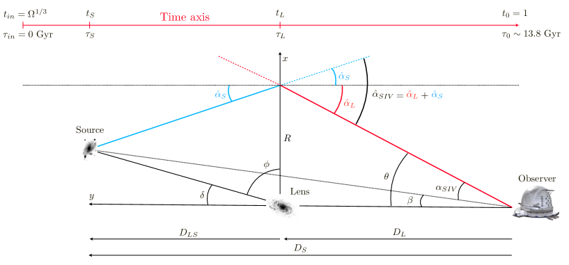
Figure 1: The geodesic of a deflected light ray. Basic sketch of the lensing geometry, with the impact parameter, $R$, in the lens plane, the polar coordinates $r$ and $\phi$, the distance $D_{\mathrm{S}}$ from the observer to the source, $D_{\mathrm{L}}$ from the observer to the lens, $D_{\mathrm{LS}}$ from the lens to the source and the $\hat{\alpha}$ deflection angles.

4 The scale invariant effects in lensing

The term $GM/R$ in the above equation is the gravitational potential which as we have seen is an invariant quantity. Thus we might wonder whether in the scale invariant context the deflection angle should not just be unchanged. Indeed, despite the fact that the potential remains the same, Eqs. (3.19) and (3.20) contain additional terms to the Einsteinian one. Also, the equation of motion in the Newtonian approximation is modified with an additional term, potentially significant in the astronomical context. Thus it makes sense to wonder whether the path of a light ray also undergoes some changes with respect to GR.

A difficulty of Eq. (3.20) is that, in addition to the independent variable $\phi$, it requires the variable $t$ to express the term $\lambda$. The two variables are related by geometrical relations on the light path. However, the result is an intricate equation, making numerical integration mandatory to evaluate relative importance of the additional terms and their impact on the deflection of light rays.

4.1 The SIV relation between redshifts and ages

To proceed to numerical integration of Eq. (3.20), we need some basic relations between the observed redshift $z$ and time $t$, which then gives the scale invariance factor $\lambda=1/t$. The expansion factor writes (2.13),

$$a(t)=\left[\frac{t^{3}-\Omega_{\mathrm{m}}}{1-\Omega_{\mathrm{m}}}\right]^{2/3},$$ (4.1)

it is directly leading to,

$$t=\left[\Omega_{\mathrm{m}}+(1+z)^{-3/2}(1-\Omega_{\mathrm{m}})\right]^{1/3}.$$ (4.2)

With $t=\Omega^{1/3}_{\mathrm{m}}+\frac{\tau}{\tau_{0}}(1-\Omega^{1/3}_{\mathrm{m}})$, one obtains the age $\tau$ in current units for a galaxy of redshift $z$,

$$\tau=\tau_{0}\frac{\left[[\Omega_{\mathrm{m}}+(1+z)^{-3/2}(1-\Omega_{\mathrm{m}})\right]^{1/3}-\Omega^{1/3}_{\mathrm{m}}}{1-\Omega^{1/3}_{\mathrm{m}}}.$$ (4.3)

This relation can also be expressed as a function of $H_{0}$, by combining with Eq. (2.20),

$$\tau=\frac{2}{H_{0}}\frac{\left[[\Omega_{\mathrm{m}}+(1+z)^{-3/2}(1-\Omega_{\mathrm{m}})\right]^{1/3}-\Omega^{1/3}_{\mathrm{m}}}{1-\Omega_{\mathrm{m}}}.$$ (4.4)

With these expressions in hand we can now associate an age to any object at any redshift.

4.2 The variations of the term $dm$

During the path of the light ray from the source, $S$, to the observer, $O$, the mass of the lens undergoes some limited variations due to the scale variations during the travel time. This results in the term $u^{3}(dm/du)$ in Eq. (3.20), coming in addition to the classical GR term $3mu^{2}$. This is because, on the light path, both $m$ and $u$ increase at the same time, so that $(dm/du)$ is positive. Alike a tidal effect, it behaves in $u^{3}=1/r^{3}$, thus being essentially located close to the lens, even more than the gravity effect itself. Since $m$ has the units of length (see Eq. 3.5), $u^{3}(dm/du)$ has the units of the inverse of a length.

Do these extra terms impact the deflection angle in the SIV context? To evaluate the effect, we consider the practical case of the remarkable strongly lensed galaxy JWST-ER1 recently observed by van Dokkum et al. [38] with the JWST. It forms a complete Einstein ring with a radius $\theta_{E}=1.54\pm 0.02$ arcseconds produced by a massive quiescent lensing galaxy at $z_{L}=1.94$ acting on a source at $z_{S}=2.98$. The total lensing mass is estimated to be $M_{\rm Tot}=6.5\times 10^{11}$ M_⊙ within a radius of 6.6 kpc at the lens redshift, while the stellar mass derived from multi-band photometry is 5.9 times lower, with $M_{\star}=1.1\times 10^{11}$ M_⊙. As stated by these authors, this is a beautiful example of a system where ”Additional mass appears to be needed to explain the lensing results, either in the form of a higher-than-expected dark matter density or a bottom-heavy initial mass function.”

We use JWST-ER1 as a test bench for our integration of the light path. This path is expressed in terms of the variable $u=1/r$ as a function the angle $\phi$, starting close to $\pi/2$ for the direction pointing to the distant source, S, all the way to the nearest point at the impact parameter where $u=1/R$ and where $\phi=0$ as can be seen from Fig. 1. We adopt a step size of $2\times 10^{-4}$ for the variable $\phi$. Tests made with smaller steps give identical results. The calculations represent an isochrone described by about 7850 points, which ensures a high accuracy of the integration. From the relation between redshifts and cosmic ages (Sect. 4.1), we have in the $t$-scale an age of the source given by $t_{\mathrm{S}}=0.5536$ and for the lens $t_{\mathrm{L}}=0.6201$, according to their redshifts. We recall that $t$ is dimensionless, with $t_{0}=1$. (The lens mass $M_{\rm Tot}$ has been taken, as well as a value $\Omega_{\mathrm{m}}=0.05$, thus assuming no dark matter. For higher values of $\Omega_{\mathrm{m}}$, the effects would be smaller than those found below). At each point defined by coordinates $(u,\phi)$ along the path of the light ray, we can then assign an age $t$ and a value $\lambda$ ($\tau$ is not needed here). We may then obtain from Eq. (2.17) the time variations of the mass as well as the term $dm/du$. In terms of numerical results, we obtain for example that in the specific case of JWST-ER1, the ratio

$$\frac{u^{3}\frac{dm}{du}}{3mu^{2}},$$ (4.5)

is equal to $6.62\times 10^{-6},\;2.25\times 10^{-7},\;6.36\times 10^{-6}$ for angles of $\phi$ = 89, 45 and 1 degree respectively. In other words, the additional term $u^{3}(dm/du)$ has a totally negligible effect on the resulting deflection angle $\hat{\alpha}_{\mathrm{S}}$. The same holds true for the second part of the path of the light ray from the lens plane, $L$, to the observer, $O$. Thus, globally this term is negligible.

4.3 The effects of the $\Lambda$ term

We now turn to the other additional term $\left(\frac{1}{c^{2}\tau^{2}_{0}}\right)\lambda\frac{d\lambda}{du}$ in Eq. (3.20), which consistently has the units of the inverse of a length. Physically, this term results from the cosmological constant, present in the exterior Schwarzschild metric (3.2). This term is thus not a direct function of the deflecting mass, but is rather associated to the specific geometry of a gravitational system where the external Schwarzschild metric applies. This term thus intervenes as an additional correction to the classical Einsteinian term. It is likely to be an extremely small quantity since $c^{2}\tau^{2}_{0}$ is the square of the ”size” of the present Universe.

The above calculations for JWST-ER1 provide the information on the magnitude of this effect on the light deflection. The ratio of term $\left(\frac{1}{c^{2}\tau^{2}_{0}}\right)\lambda\frac{d\lambda}{du}$ to the classical Einsteinian term $3mu^{2}$ is generally negligible. For example, it is as small as $1.38\times 10^{-5}$, $1.16\times 10^{-8}$, and $2.30\times 10^{-7}$ for angles of $\phi=89,45$ and 1 degree respectively. Thus, except near the source the above ratio is smaller than the term due to the mass variations. The consequences of the term $\left(\frac{1}{c^{2}\tau^{2}_{0}}\right)\lambda\frac{d\lambda}{du}$ on the deflection angle $\hat{\alpha}_{\mathrm{S}}$ is also negligible in all possible current situations, and the same occurs for the second part of the light path, i.e. described by $\hat{\alpha}_{\mathrm{L}}$. Only at the orgin when the term $c\tau_{0}$ tends to zero could it have played some role in the light path.

4.4 General case of light deflection

We have studied the nice case of JWST-ER1, but what about lensing by larger masses, such as galaxy clusters? As far as the mass variations are concerned, i.e., $u^{3}\frac{dm}{du}$, we see that its ratio to the Einsteinian term $3mu^{2}$ changes as $\frac{1}{3}\frac{dm}{m}\frac{u}{du}$. Thus, as the relative change of the mass $dm/m$ is independent of the mass (since $dm\sim m$), our conclusion applies to any mass, thus including clusters of galaxies.

The deflection angle is essentially independent from scale invariant effects, as shown above.This result is consistent with the fact that an angle is a scale-invariant quantity as long as the cosmological evolution of the space-time is homogeneous and isotropic. The present detailed analysis demonstrates that the local inhomogeneity and anisotropy of the space-time created by a mass element in the scale invariant context introduce only minor differences in the light deflection as compared to standard GR. These effects are clearly not sufficient to account for the large mass difference observed in JWST-ER1 [38] between the masses from the lensing effect and from the observed luminosity.

This confirms that the masses obtained by the lensing effect are a most remarkably model-independent result, in particular they are independent of scale invariant effects and on the cosmological models as long they are homogenous and isotropic. This result in itself is a fundamental one: the geodesics of light in scale-invariance theory do not change with respect to standard GR assumptions.

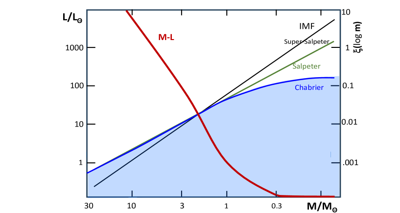
Figure 2: The red thick curve represents the mass-luminosity relation on the zero-age sequence [18], according to the scale indicated on the left vertical axis. The other curves describe various IMF: Chabrier [6], Salpeter with $x=1.35$ [35] and the so-called Super-Salpeter by [38], according to the scale indicated on the right vertical axis. Note that in $\xi(\log m)$ the log is decimal. The Figure is inspired from [38].

5 The origin of the discrepancy between the stellar and lensing masses

Since the gravitational lensing deflection angle appear to be free from scale invariant effects, we may now turn to the impact of scale invariance on lens mass estimates in the Einstein radius, as derived from photometry or spectroscopy of the lens.

5.1 The emblematic case of JWST-ER1s

We consider here again the remarkable case of JWST-ER1 and its high lensing-to-stellar mass ratio of $\sim 6$ according to van Dokkum et al. [38] and already presented in Sect. 4.2. With a lens redshift $z_{\mathrm{L}}=1.94$, it is a textbook example of a distant massive quiescent galaxy with a low star formation rate. It has an age of $\tau_{\mathrm{L}}=1.9^{+0.3}_{-0.6}$ Gyr, implying that relatively low mass stars dominate the stellar population of the lensing galaxy. Its unitless age is $t_{\mathrm{L}}=0.62$ (cf. Eq. 4.2), taking $\Omega_{\mathrm{m}}=0.05$, i.e. assuming no dark matter (the Big-Bang occured at $t_{\mathrm{in}}=\Omega^{1/3}_{\mathrm{m}}$, i.e. 0.3684). According to Eq. (2.17), this would imply that the inertial and gravitational masses in JWST-ER1 is equal to a fraction 0.62 of its present value. Incidentally this might also contribute to the observed compactness of the early galaxies. This means that the stellar mass distribution in JWST-ER1 may be shifted to lower masses with respect to today’s distribution. Interestingly enough, the consequences of this shift have rather similar effects to those of the solution proposed by van Dokkum et al. [38] to solve the mass discrepancy between the mass infered from the lens luminosity and its lensing mass, $M_{Tot}=6.5^{+3.7}_{-1.5}\times 10^{11}\;M_{\odot}$. They suggest a shift from Chabrier’s IMF [6], which has relatively few low-mass stars giving a mass of $M_{*}=1.1^{+0.2}_{-0.3}\times 10^{11}\;M_{\odot}$, to a very bottom-heavy IMF called ”Super-Salpeter IMF” giving a mass of $M_{*}=4.0^{+0.6}_{-0.8}\times 10^{11}\;M_{\odot}$. The standard Salpeter IMF gives an intermediate value of $M_{*}=2.0^{+0.5}_{-0.5}\times 10^{11}\;M_{\odot}$. Fig. 2 illustrates the different IMF assumptions.

The rather ad-hoc shift produced by the assumption of a Super-Salpeter IMF leads to a large increase of the mass-to-light ratio since it assumes a relatively larger fraction of lower stellar masses, with lower luminosities (Fig. 2). Even with the Super-Salpeter assumption, a significant fraction of dark matter is still necessary, $M_{\mathrm{DM}}=2.6^{+1.6}_{-0.7}\times 10^{11}\;M_{\odot}$, to explain the observed Einstein radius of this system.

The observed luminosity $L_{\mathrm{obs}}$ reflects the true mass of the stars as they are at any given age. For an age of $\tau_{\mathrm{L}}=1.9^{+0.3}_{-0.6}$ Gyr assigned by Prospector, the turnoff mass is around 1.7 $M_{\odot}$ [18]. This corresponds well to a general remark by [17] that most of the light of the old stellar populations of galaxies comes from stars with a mass in the range of $[1-2]$ M_⊙. A shift in mass by a factor 0.62 for JWST-ER1, as predicted by the scale-invariant theory, implies a significant difference in the relative number frequency of stars as compared to the standard case.

Let us estimate the effect of such a shift on the average mass-luminosity ratio $\langle M/L\rangle$ of a galaxy by some simple relations. As an example, we take an initial mass function $\xi(\ln m)$ of the Salpeter form [35],

$$\xi(\ln m)=\frac{dN}{d\ln\,m}=\frac{dN}{dm}m=Am^{-x},\quad\mathrm{or}\;\frac{dN}{dm}=Am^{-(1+x)},$$ (5.1)

with $x=1.35$ (see Fig. 2). The mass of the galaxy then writes,

$$M_{gal}=\int\frac{dN}{dm}m\,dm=A\int m^{-x}dm=\;\mid\frac{A}{-x+1}({m_{m}}^{-x+1})\mid_{m_{min}}^{m_{max}}\;=Am_{m},$$ (5.2)

where $A$ is a normalization constant and where $m_{m}$ is the mean mass over the mass spectrum. This mean mass is $m_{m}=$13.7 M_⊙ for a mass interval that extends from $m_{min}=0.01$ to $m_{max}=100$ M_⊙. If we call $\ell(m)$ the luminosity of a star of mass $m$, the stellar mass-luminosity relation writes, $\ell(m)=B\,m^{\alpha}$, where $B$ is another normalization constant. The luminosity of a galaxy becomes,

$$L_{gal}=\int\ell(m)\frac{dN}{dm}dm=AB\int m^{\alpha}\,m^{-(x+1)}dm=\;\mid\frac{AB}{\alpha-x}{m}^{\alpha-x}\mid_{m_{min}}^{m_{max}}\;=AB\,m_{L},$$ (5.3)

where $m_{L}$ is the mean mass over the luminosity distribution. Typical values are 1.7-1.8 M_⊙. Thus, the mean mass-luminosity ratio of a galaxy is scaling like,

$$\left\langle\frac{M}{L}\right\rangle=\frac{(\alpha-x)}{B(1-x)}m_{m}^{1-x}\;m_{L}^{x-\alpha}.$$ (5.4)

If all the masses are reduced by the same factor, this factor applies both to $m_{m}$ and $m_{L}$. The values of $\alpha$ in the range of 1 to 2 M_⊙ considered earlier is quite large, hence making $\ell$ a very steep function of $m$, as shown in Fig. 2. We have, following Maeder [18]

$$\ell\sim m^{\alpha}, \hskip 5.0pt\alpha=3.69, \hskip 5.0ptm\in[9-2]\;M_{\odot}$$ (5.5)

$$\hskip 5.0pt\alpha=4.56, \hskip 5.0ptm\in[2-1]\;M_{\odot}$$

$$\hskip 5.0pt\alpha=4.00, \hskip 5.0ptm\in[1-0.6]\;M_{\odot}$$

The individual stellar mass-luminosity ratios $m/\ell$ are varying with power $(1-\alpha)$ of the mass $m$, while Eq. (5.4) shows that the factors are different when integrated over the mass spectrum of a galaxy. Now, we can see what is doing a change of the mass by a factor $f=0.62$, (this factor is the ratio $t/t_{0}=t$ corresponding to the reshift $z=1.94$ of the lens in JWST-ER1). The ratio of the modified overall mass-luminosity ratio to the standard unmodified case is,

$$\frac{\left\langle\frac{M}{L}\right\rangle_{f}}{\left\langle\frac{M}{L}\right\rangle_{\mathrm{std}}}\sim f^{1-x}\;f^{x-\alpha}=f^{1-\alpha}.$$ (5.6)

Interestingly enough, for a change of all masses by the same factor $f$, we come back to the same dependence as given by the simple individual stellar expression $(m/\ell)\sim m^{1-\alpha}$; for other changes of the mass distribution the full expression has evidently to be kept in. For of factor $f=0.62$ and $\alpha=4.56$, we get a value of 5.48 for the ratio expressed in Eq. (5.6). Thus, the real mass-luminosity ratio may be about a factor of 5.48 higher than the assumed one, which accounts for most of the difference between the mass observed from lensing and the mass derived from the luminous matter.

The so-called super-Salpeter IMF with $x\approx 1.65$ applied by van Dokkum et al. [38] increases the total mass by a factor of about 4 compared to Salpeter’s. In the scale invariant context, such a hypothesis of a very bottom-heavy mass distribution, just opposed to the Chabrier one, is not necessary. A mass distribution close to the Chabrier IMF naturally accounts for the lensing mass without calling for dark matter. Thus, while the mass estimates by lensing are totally unaffected by scale invariant effects, it is not the case for the spectrophotometric determinations, which may be severely biased for distant galaxies, such as JWST-ER1.

5.2 The SLACS sample of galaxies

To complement the above results for JWST-ER1, we turn towards the Sloan Lens ACS (SLACS) survey by Bolton [3] which is one of the largest and most homogeneous data set of galaxy-scale lenses, containing about 100 lenses analysed by Auger et al. [1]. One of the aim of the survey was to study the distribution of luminous and dark matter out to redshift $z\approx 0.5$. It is based on multi-band imaging with ACS, WFC and NICMOS on the HST. The observations have been analysed with a lens model using an isothermal ellipsoid mass distribution, allowing high precision measurements of the mass within the Einstein radius for each lens. The resulting mass estimates have been found unbiased compared to the estimates from SDSS photometry and are in the range $10^{10.5}<M<10^{11.8}$ $M_{\odot}$, with a typical statistical error of 0.1 dex. The mean mass-luminosity ratio of the sample of the galaxies considered in the SLACS sample is about $\langle M/L\rangle=8.7$. Such a ratio corresponds to a representative stellar mass of about 1.84 $M_{\odot}$, not much different from the case of JWST-ER1.

The survey provides for each lens the fractions $f^{Chab}_{*,Ein}$ and $f^{Salp}_{*,Ein}$ of the stellar mass within the Einstein radius for the Chabrier and Salpeter IMFs [6, 35] with respect to the total lensing mass. As stated by [1], these fractions are independent of any priors from lensing, so that in some cases fractions higher than 1 were obtained. The survey provides a mean stellar mass fraction within the Einstein radius of $\langle f^{Chab}_{*,Ein}\rangle=0.4$ with a rms scatter of 0.1 for the Chabrier IMF; for the Salpeter’s IMF the mean is $\langle f^{Salp}_{*,Ein}\rangle=0.7$ and a rms scatter of 0.2.

In the data of Table 3 and 4 by [1], we select two samples of lenses at different redshifts: for low redshifts, we select systems with $z_{\mathrm{L}}\leq 0.15$ and another sample with $z_{\mathrm{L}}\geq 0.35$. This split in two bins of $\Delta z=0.15$ is a compromise between the need to have two different mean redshifts and also a sufficient number of galaxies in each sub-sample. The results are shown in Table 1. We see that the stellar mass fractions are higher for low $z$-interval, by $\Delta f_{*}=0.092$ for the Chabrier IMF and by $\Delta f_{*}=0.166$ for the Salpeter IMF. These differences are rather small, of the same order as the uncertainties, unlike the high-$z$ case of JWST-ER1. The standard deviations of the different fractions are also given in Table 1, allowing a test of significance.

Combining the two values for each IMF, we get $\sigma=0.135$ for the difference $\Delta f_{*}=0.449-0.357=0.092$ of the $\langle f^{Chab}_{*,Ein}\rangle$ values. For a normal distribution, this corresponds to a probability of 50.4% that the difference is significant. For $\langle f^{Salp}_{*,Ein}\rangle$, the difference is $\Delta f_{*}=0.792-0.626=0.166$ and $\sigma=0.239$, giving a probability of 51.2%. Thus, the differences are possible, but also well compatible with a random realization. The ages $t$ corresponding to the mean redshifts $z=0.114$ and $z=0.383$ of the two samples are respectively $t=0.8591$ and $t=0.9502$ in the dimensionless time scale, again for $\Omega_{\mathrm{m}}=0.05$. According to Eq. (2.17), masses scale like $t$, which implies an increase by about 10% between the two redshifts. The observations effectively suggest an increase of the same order of magnitude, which is quite satisfactory. Nevertheless the observational uncertainties preclude from establishing this correspondence on a firm statistical ground.

As in the case JWST-ER1, the Salpeter IMF gives masses in better agreement with observations than Chabrier’s IMF: the mass estimates from the photometric observations at $\langle z\rangle=0.114$ give a mass equal to 79.2% of the total lensing mass. If we account, as above for JWST-ER1, for the shift of the Salpeter IMF resulting from the smaller masses in scale invariance, we need to rescale the stellar fraction in the Einstein radius following Eq. (5.6). For the low redshift bin $\langle z\rangle=0.114$, we obtain today’s corresponding value of the stellar mass fraction of $\langle f^{Salp}_{SIV}\rangle=0.792\times 0.9502^{-3.56}=0.95$. For the high reshift bin, $\langle z\rangle=0.383$, we obtain $\langle f^{Salp}_{SIV}\rangle=0.626\times 0.8591^{-3.56}=1.07$. These two fractions, very close to 1.0, mean that when the shift in mass due to scale invariance is accounted for, the stellar masses from photometry/spectroscopy and for a standard IMF are also here remarkably close to the masses from lensing, in support of the present interpretation.

Table 1: Analysis of the SLACS Survey: the mean stellar mass fractions within the Einstein radius, $\langle f^{Chab}_{*,Ein}\rangle$ and $\langle f^{Salp}_{*,Ein}\rangle$ are given for Chabrier and Salpeter IMFs respectively as well as the corresponding standard deviations among the two subsamples of redshifts. The column $\langle f^{Salp}_{SIV}\rangle$ gives the theoretical value of the stellar mass fraction with Salpeter’s IMF obtained after accounting for the scale invariant correction. The last number gives the number of galaxies in each sub-sample.

$\mathrm{Redshift\;interval}$	$\langle z\rangle$	$\langle f^{Chab}_{*,Ein}\rangle$	$\langle f^{Salp}_{*,Ein}\rangle$	$\sigma(f^{Chab}_{*,Ein})$	$\sigma(f^{Salp}_{*,Ein})$	$\langle f^{Salp}_{SIV}\rangle$	$N$
$0\leq z\leq 0.15$	0.114	0.449	0.792	0.110	0.197	0.95	17
$0.3\leq z\leq 0.5$	0.383	0.357	0.626	0.079	0.136	1.07	10

6 Discussion and proposed lensing tests

On the basis of the JWST-ER1 and the SLACS studies, we have seen that the observed differences between the stellar masses from photometry and from lensing are increasing with redshifts. We show that scale invariance theory can reconcile the two mass estimates, both at low and high redshifts.

Of note, different results obtained with GR and dark matter (FDM) seem to severely contradict each other. At high redshift, like in JWST-ER1, the DM component vastly dominates the lens mass, to the point that a super-Salpeter IMF is invoked in addition to a DM halo with extreme densities. Recently Kong et al. [16] attempted to alleviate the DM density by invoking the presence of self-interacting DM. But their overall conclusion that JWST-ER1 is an extreme lens in terms of DM content at high redshift comes in contrast with several recent studies on rotation curves of galaxies by Nestor Shachar [28] that corroborate previous results by the Genzel group, showing that much less dark matter is needed in GR at high reshift than at low redshift. For example, only a fraction of about 17% of the typical value appears to be remaining in galaxies at $z=2.44$ [28], in sharp contrast with JWST-ER1.

The present work focuses on the comparison of the total lensing mass of galaxies and the total luminous mass in GR and in scale invariance. It suggests that, in scale invariance, the total luminous mass is sufficient to explain the observed deflection angle without the need of dark matter, given the observational errors. This paves to the way to many other more detailed tests involving lensing in scale invariance:

• Pixel-level modeling: state-of-art modeling of lens galaxies decomposes their mass into luminous mass plus dark matter NFW halo [29, 30]. This allows to model HST images of lensing systems down to the noise level. A strong test for scale invariance lensing would be to attempt the same without the DM component, just using the light map of the lens and converting it into mass following the recipes of the present work.

• Lens dynamics: dynamical information is available for some strong lens systems, including SLACS. Joint lens/dynamical analysis of strong lenses in the context of scale invariance would further test the theory. This is not straightforward, however, as the Viriel theorem does not apply directly in scale invariance and requires to account for the additional acceleration due to scale invariance.

• Time delay cosmography: Time delays in lensed quasars can be converted into an $H_{0}$ measurement, provided the slope of the lens mass is known (or modeled) at the position of the quasar images [2]. In scale invariance and a no-DM lens model, the slope of the mass becomes extremely well constrained as the degeneracy between invible DM and well-visible baryons is lifted. This may have an impact on the infered $H_{0}$ value and in turn on the Hubble tension. It will also be a strong test for scale invariance as, with no DM, the Mass Sheet Degeneracy is also fully broken [37]. The $H_{0}$ values infered by lensing time delays, in scale invariance, will directly result from the slope of the luminous mass at the positions of the lensed quasar images. This is directly constrained by deep HST or JWST imaging.

• Lensing by edge-on spirals: The luminous mass in edge-on galaxies is of course extremely elliptical. In scale invariance the mass is dominated by baryons (or even fully accounted for by baryons) and therefore the difference in lensing configurations between no-DM scale invariance models and standard models dominated by a fairly spherical halo, should offer great discriminating power between the two theories. In fact, hints of such behaviour may have been found already, for example with the spectacular case of J220132.8-320144 where some of the lensed images predicted by standard models with DM are missing from HST imaging data [7].

• Weak lensing: Weak lensing mass maps of galaxy clusters are unaffected by scale invariance, just as for strong lensing. However, as for strong lensing, scale invariance changes the infered luminous mass. It will therefore be crucial to compare the weak lensing mass infered for galaxy clusters to that infered from spectroscopy for all galaxy members, for example with ultra deep integral field spectroscopy. Additionally, and as shown in [22], the scale invariance mass infered from galaxy velocities should also be consistent with the scale-invariant luminous mass.

The above proposed tests are beyond the scope of the present paper but most observational material to implement them do exist and will be used in the near future.

7 Conclusions

Detailed calculations of the geodesic equation to study deviation of light rays passing a massive object have been developed in the scale invariant theory. The inhomogeneity and anisotropy of space-time associated to the presence of a lensing galaxy generate two additional terms in the equation of the geodesics with respect to General Relativity. However, in practice, numerical integration of the geodesics performed specifically for the Einstein ring JWST-ER1 with its lensing galaxy at $z_{L}=1.94$ indicates that the change in deflection angle is typically a fraction $\mathcal{O}$($10^{-6}$) of that predicted by GR. The lensing deflection can therefore be considered as independent from scale invariant effects. However, while scale invariance has no effect on the photons’ geodesics themselves, the actual impact of scale invariance resides in the interpretation and use of the mass-luminosity relation of the stellar population in the lens galaxy and of its IMF.

References

- Auger et al. [2009] Auger, M.W., Treu, T., Bolton, A.S. et al., The SLOAN lens ACS Survey. XI. Colors, lensing and stellar masses of early-type galaxies., ApJ, 705, 1099 (2009)
- Birrer et al. [2022] Birrer, S., Millon, M., Sluse, D., et al., Time-Delay Cosmography: Measuring the Hubble Constant and other cosmological parameters with strong gravitational lensing arXiv2210.10833, in press in Space Science Review (2022)
- Bolton et al. [2008] Bolton, A. et al., The Sloan Lens ACS Survey. V. The Full ACS Strong-Lens Sample, ApJ, 682, 964 (2008)
- Bouvier & Maeder [1978] Bouvier, P., Maeder, A., Consistency of Weyl’s Geometry as a Framework for Gravitation, Astrophys. Space Science, 54, 497 (1978)
- Canuto et al. [1977] Canuto, V., Adams, P. J., Hsieh, S.-H., & Tsiang, E., Scale-covariant theory of gravitation and astrophysical applications, PhRvD, 16, 1643 (1977)
- Chabrier [2003] Chabrier, G., Galactic Stellar and Substellar Initial Mass Function, Publ. Astron. Soc. Pacific,. 115, 763 (2003)
- Chen [2013] Chen, J., Lee, S.K., Castander, F.-J., et al., Missing Lensed Images and the Galaxy Disk Mass in CXOCY J220132.8-320144, ApJ 769, 81 (2013)
- Dirac [1973] Dirac, P. A. M., Long Range Forces and Broken Symmetries, Proceedings of the Royal Society of London Series A, 333, 403 (1973)
- Dirac [1974] Dirac, P. A. M., Cosmological Models and the Large Numbers Hypothesis, Proceedings of the Royal Society of London Series A, 338, 439 (1974)
- Eddington [1919] Eddington, A.S., The total eclipse of 1919 May 29 and the influence of gravitation on light, The Observatory, 42, 119 (1919)
- Eddington [1923] Eddington, A.S., The Mathematical Theory of Relativity, Chelsea Publ. Co. New York, 266 p. (1923)
- Einstein [1918] Einstein, A., Sitzung Berichte der Königlich Preussischen Akademie des Wissenschaften (Berlin), p. 478 (1918)
- Hernandez et al. [2022] Hernandez, X., Cookson, S., Cortes, R.A.A., Internal kinematics of Gaia eDR3 wide binaries, MNRAS 502, 2304 (2022)
- Johnson et al. [2021] Johnson, B.D., Leja, J., Conroy, C., Speagle, J.S., Stellar Population Inference with Prospector, ApJ. Suppl. Ser. 254, 22 (2021)
- Jesus [2018] Jesus, J.F., Exact solution for flat scale-invariant cosmology, Rev. Mex. Astron. Astrophys. 55, 17 (2018)
- Kong et al. [2024] Kong, D., Yang, D., Yu, H.-B., CDM and SIDM Interpretations of the Strong Gravitational Lensing Object JWST-ER1 arXiv2402.15840 (2024)
- Longair [1998] Longair, M.S., Galaxy Formation, Springer Bewrlin, 536 p. (1998)
- Maeder [2009] Maeder, A., Physics, Formation and Evolution of Rotating Stars, Springer Verlag, 829 p. (2009)
- Maeder [2017a] Maeder, A., An Alternative to the LambdaCDM Model: The Case of Scale Invariance, Astrophys. J., 834, 194 (2017a)
- Maeder [2017c] Maeder, A., Dynamical Effects of the Scale Invariance of the Empty Space: The Fall of Dark Matter?, Astrophys. J., 849,158 (2017c)
- Maeder [2023] Maeder, A., MOND as a peculiar case of the SIV theory, MNRAS, 520, 1447 (2023)
- Maeder [2024] Maeder, A. 2024, submitted
- Maeder & Bouvier [1979] Maeder, A., Bouvier, P., Scale invariance, metrical connection and the motions of astronomical bodies, Astron. Astrophys., 73, 82 (1979)
- Maeder and Gueorguiev [2019] Maeder, A.; Gueorguiev, V.G., The growth of the density fluctuations in the scale-invariant vacuum theory, Physics of the Dark Universe, 25, 100315 (2019)
- Maeder and Gueorguiev [2021a] Maeder, A.; Gueorguiev, V.G., Scale invariance, horizons, and inflation, MNRAS, 504, 4005 (2021a)
- Maeder and Gueorguiev [2023] Maeder, A.; Gueorguiev, V.G., Action Principle for Scale Invariance and Applications (Part I), Symmetry, 15, 1966 (2023)
- Milgrom [2013] Milgrom, M., Testing the MOND Paradigm of Modified Dynamics with Galaxy-Galaxy Gravitational Lensing, Phys. Rev. Letters, 111, 1105 (2013)
- [28] Nestor Shachar, A., Price, S.H., Forster Schreiber, N. M. et al. RC100: Rotation Curves of 100 Massive Star-forming Galaxies at z = 0.6-2.5 Reveal Little Dark Matter on Galactic ScalesRC100: Rotation Curves of 100 Massive Star-forming Galaxies at z = 0.6-2.5 Reveal Little Dark Matter on Galactic Scales, ApJ 944, 78 (2023)
- Suyu et al. [2013] Suyu, S., Auger, M., Hilbert, S., et al., Two Accurate Time-delay Distances from Strong Lensing: Implications for Cosmology, ApJ 766, 70 (2013)
- Suyu et al. [2014] Suyu, S., Treu, T., Hilbert, S., et al., Cosmology from Gravitational Lens Time Delays and Planck Data ApJ 788, L35 (2014)
- Old et al. [2018] Old, L., Wojtak, R., Pearce, F.R. et al., Galaxy Cluster Mass Reconstruction Project - III. The impact of dynamical substructure on cluster mass estimates, MNRAS, 475, 853 (2018)
- Planck Collaboration [2020] Planck Collaboration 2020, Aghanim, N., Akrami, Y. Ashdown, M., Planck 2018 results. VI. Cosmological parameters, Astron. Astrophys. 641, A6 (2020)
- Rindler [1956] Rindler, W., Visual horizons in world models, MNRAS, 116, 662 (1956)
- Rindler [1969] Rindler, W., Essential relativity. Special, general and cosmological, Springer Verlag, Heidelberg, 284 p. (1969)
- Salpeter [1955] Salpeter, E., The Luminosity Function and Stellar Evolution, ApJ, 121,161 (1955)
- Tolman [1934] Tolman, R.C., Relativity Thermodynamics and Cosmology, Oxford At the Clarendon press, 502 p. (1934)
- Treu & Shajib [2023] Treu, T., Shajib, A., Strong Lensing and , arXiv2307.05714 (2023)
- van Dokkum et al. [2024] van Dokkum, P., Brammer, G., Wang, B. et al., A massive compact quiescent galaxy at z=2 with a complete Einstein ring in JWST imaging, Nature Astronomy, 8, 119 (2023)
- Weinberg [1972] Weinberg, S., Gravitation and Cosmology: Principles and applications of the General Theory of Relativity, John Wiley & Sons, Inc, New York, London, Sydney, Toronto (1972)
- Weyl [1923] Weyl, H., Raum, Zeit, Materie. Vorlesungen über allgemeine Relativitätstheorie. Re-edited by Springer Verlag, Berlin, 1970 (2023)