A Generalized Framework with Adaptive Weighted Soft-Margin for Imbalanced SVM Classification

Abstract

Category imbalance is one of the most popular and important issues in the domain of classification. In this paper, we present a new generalized framework with Adaptive Weight function for soft-margin Weighted SVM (AW-WSVM), which aims to enhance the issue of imbalance and outlier sensitivity in standard support vector machine (SVM) for classifying two-class data. The weight coefficient is introduced into the unconstrained soft-margin support vector machines, and the sample weights are updated before each training. The Adaptive Weight function (AW function) is constructed from the distance between the samples and the decision hyperplane, assigning different weights to each sample. A weight update method is proposed, taking into account the proximity of the support vectors to the decision hyperplane. Before training, the weights of the corresponding samples are initialized according to different categories. Subsequently, the samples close to the decision hyperplane are identified and assigned more weights. At the same time, lower weights are assigned to samples that are far from the decision hyperplane. Furthermore, we also put forward an effective way to eliminate noise. To evaluate the strength of the proposed generalized framework, we conducted experiments on standard datasets and emotion classification datasets with different imbalanced ratios (IR). The experimental results prove that the proposed generalized framework outperforms in terms of accuracy, recall metrics and G-mean, validating the effectiveness of the weighted strategy provided in this paper in enhancing support vector machines.

1 Introduction

Support Vector Machine (SVM), a typical statistical learning method, was first proposed by Vapnik and Cortes in 1995 [1]. SVM has gained significant popularity as a classification and regression algorithm. It has been used in various real-world problems widely and successfully, including particle recognition, text classification [2, 3, 4], visual recognition [5], feature selection[6, 7], and bioinformatics [8]. SVM encounters various obstacles, including the incorporation of previous knowledge from the datasets [9, 10] and the identification of a suitable kernel function for mapping the datasets to a separable space of high dimensions [11], and expediting the resolution of quadratic programming (QP) problems [12, 13, 14]. Our exclusive focus lies in utilizing SVM to address the challenges posed by large-scale imbalanced datasets. In doing so, we employ the technique of assigning distinct weights to individual samples. The SVM classification hyperplane is uniquely determined by support vectors (SVs). A sample that satisfies $y_{i}f(x_{i})=1$ is called a boundary support vector. The two planes that are parallel to the optimal classification hyperplane and intersect the boundary support vector are referred to as classification interval hyperplanes.

$$H_{1}:f(x_{i})=1,y_{i}=+1$$ (1)

$$H_{2}:f(x_{i})=-1,y_{i}=-1$$

The error support vector lies between the hyperplanes $H_{1}$ and $H_{2}$ in the classification interval. Once the optimal classification hyperplane is acquired, the decision function can be expressed as

$$f(x)=\text{sgn}(w^{T}x+b)$$ (2)

where $\text{sgn}(\cdot)$ represents the sign function.

Noise frequently contaminates the training data in several practical engineering applications. Furthermore, certain data points within the training dataset are erroneously positioned into the feature space alongside other categories, which are referred to as outliers. As indicated in [15] and [16], outliers frequently transform into support vectors that have higher Lagrangian coefficients throughout the training process. The classifier created using the support vector machine exclusively depends on support vectors. The existence of outliers or noise in the training set leads to a large deviation of the decision border from the ideal plane, when using the standard SVM training technique. This high sensitivity of SVM to outliers and noise is a consequence of this deviation. This work proposes the inclusion of weights to showcase the contributions of various samples.

Our primary focus is on the fundamental problem of standard SVMs. Descent techniques can be employed to minimize the objective function of a conventional SVM, which is known for its high convexity. Nevertheless, descent methods necessitate accurate calculation of the gradient of the goal function, a task that is frequently arduous. The Stochastic Gradient Descent (SGD) method addresses this issue by employing unbiased gradient estimates using tiny data samples [17, 18]. It is the primary approach for solving large-scale stochastic optimization issues. Nevertheless, the practical attractiveness of SGD approaches remains restricted due to their need for a substantial number of iterations to achieve convergence. Indeed, stochastic gradient descent (SGD) exhibits sluggish convergence due to its reliance on gradients, a drawback that is further amplified when gradients are substituted with random approximations. Various stochastic optimization strategies have been employed thus far to address SVM models. Aside from first-order techniques such as stochastic gradient descent (SGD), second-order approaches are also extensively employed. Second-order stochastic optimization methods impose greater demands on functions compared to first-order methods, as they are capable of quadratic differentiation. Consequently, studying these approaches is a demanding task. Second-order stochastic optimization methods inherently address the issues of limited precision and sluggish convergence that are associated with first-order approaches. This paper considers solving SVM using second-order stochastic optimization methods to further reduce the impact of outliers and dataset imbalance while ensuring accuracy.

In this paper, we introduce a novel generalized framework with adaptive weight function for imbalanced SVM classification (AW-WSVM). The approach involves assigning weights to distinct samples and updating these weights based on the position of the hyperplane. Our main contributions are as follows:

1. This work presents a novel weighting technique for support vector machines. The contribution of a training sample to the optimal classification hyperplane is determined by its distance from the hyperplane. Specifically, the closer the sample is to the hyperplane, the higher its weight is set, whereas the weight is smaller for samples that are farther away. We suggest the implementation of a novel weight function. The weight function is adaptive, and it can adjust itself with the change of hyperplane. It is deemed appropriate to assume that the weight setting follows a Gaussian distribution and that the impact of distance on the weight is stressed.

2. We enhance the unconstrained soft margin support vector machine. When the weight increases, the hinge loss function approaches zero to minimize the objective function, thus dividing the samples correctly.

3. We preprocess the data in each iteration. According to the directionality of the distance, we can select the noise data according to certain rules and eliminate it in the next training.

4. Employ the weighting technique we suggested in conjunction with various optimization algorithms, and conduct experiments using datasets with different characteristics. In the field of emotion classification, we have done many experiments under different imbalanced ratios. The results demonstrate that the suggested weighting technique can enhance the performance of SVM even more.

The remaining sections of this paper are structured in the following manner. Section 2 provides a concise overview of the recent literature on the classification of imbalanced data. Section 3 presents the introduction of a novel weighted method. Section 4 involves conducting experiments on various datasets by integrating different algorithms with our suggested weighting technique. The discussion and conclusions can be found in section 5.

2 Related Work

2.1 Imbalanced Data

Data imbalances occur in the real world, often leading to overfitting. Faced with the problem of imbalance in SVM, there are two popular solutions. The first is to reconstruct the training points. Increase the number of points of a few classes in different ways (oversampling) or decrease the number of points of a majority class (undersampling) [19, 20]. The second is to introduce appropriate weight coefficients into the loss function. The error cost or the decision threshold of imbalanced data is adjusted to increase the weight of the minority class and reduce the weight of the majority class to achieve balance. An initial approach to incorporating weighting into SVM is through the use of fuzzy support vector machine (FSVM) [21]. Fuzzy SVM assigns different fuzzy membership degrees to all samples in the training set, and retrains the classifier. Shao et al.[22] introduced an extremely efficient weighted Lagrangian twin support vector machine (WLTSVM) that utilizes distinct training points to create two nearby hyperplanes for the classification of unbalanced data. Fan et al. [23] proposed an improved method based on FSVM to determine fuzzy membership by class determinism of samples, so that distinct samples can provide different contributions to the classification hyperplane.Kang et al. [24] introduced a downsampling method for Support Vector Machines (SVM) that uses spatial geometric distances. This method assigns weights to the samples depending on their Euclidean distance from the hyperplane. The weights highlight the samples’ influence on the decision hyperplane.

2.2 Outliers of SVM

In the real world, datasets often possess substantial size and exhibit imbalances, hence posing challenges to the problem-solving process. Yang et al.[25] proposed Weighted Support Vector Machine (WSVM), which addresses the issue of anomaly sensitivity in SVM by assigning varying weights to different data points. The WSVM approach utilizes the kernel-based Probability c-means (Kpcm) algorithm to provide varying weights to the primary training data points and outliers. Wu et al.[26] introduced the Weighted Margin Support Vector Machine (WMSVM), a method that combines prior information about the samples and gives distinct weights to different samples. Zhang et al. [27] proposed a Density-induced Margin Support Vector Machine (DMSVM), for a given dataset, DMSVM needs to extract the relative densities of all training data points. The densities can be used as the relative edges of the corresponding training data points. This can be considered as an exceptional instance of WMSVM. In [28], particle swarm optimization (PSO) is used for the time weighting of SVM. Du et al.[29] introduced a fuzzy-compensated multiclass SVM approach to improve the outlier and noise sensitivity issues, proposing how to dynamically and adaptively adjust the weights of the SVM. Zhu et al.[30] introduced a weighting technique based on distance, where the weights are determined by the proximity of the nearest diverse sample sequences, referred to as extended nearest neighbor chains. The paper [31] presents a novel approach called the weighted support vector machine (WSVM-FRS), which involves incorporating weighting coefficients into the penalty term of the optimization problem. Inadequate samples possess minimal weights, while significant samples possess substantial weights.

2.3 Stochastic Optimization Algorithm for SVM

Gradient-based optimization techniques are widely used in the development of neural systems and can also be applied to solve SVM. First-order approaches are commonly employed due to their straightforwardness and little computational cost. Some examples of optimization algorithms are stochastic gradient Descent (SGD)[32], AdaGrad[33], RMSprop[34], and Adam[35]. Although the first-order approach is easy to understand, its slow convergence is a significant disadvantage. Utilizing second-order bending information enables the improvement of convergence. The Broyden-Fletcher-Goldfarb-Shanon (BFGS) approach has garnered significant attention and research in the training of neural networks. Simultaneously, an increasing number of scholars are employing the BFGS algorithm to address Support Vector Machine (SVM) problems. However, a significant drawback of the second-order technique is its reliance on substantial processing and memory resources. Implementing quasi-Newtonian methods in a random environment poses significant challenges and has been a subject of ongoing research. The Online BFGS (oBFGS) approach, mentioned [36], is a stochastic quasi-Newtonian method that has demonstrated early stability. In contrast to BFGS, this method eliminates the need for line search and alters the update of the Hessian matrix. An analysis is conducted on the worldwide convergence of stochastic BFGS, and a novel online L-BFGS technique is introduced [37]. A novel approach is suggested, which involves subsampling Hessian vector products and collecting curvature information periodically and point-by-point. This method can be classified as a stochastic quasi-Newtonian method [38]. In [39], the authors introduce a stochastic (online) quasi-Newton method that incorporates Nesesterov acceleration gradients. This strategy is applicable in both complete and limited memory formats. The study demonstrates the impact of various momentum rates and batch sizes on performance.

In the following sections, we apply the proposed framework to SGD, oBFGS and oNAQ to do comparative experiments. We pay more attention to these three algorithms, SGD and oBFGS are summarized in Algorithm 1 and Algorithm 2 respectively. ONAQ will be discussed in the third section.

Algorithm 1 SGD Method[32]

1:minibatch $X_{k}$, $k_{max}$ and learning rate $\epsilon$

2:$\mathbf{w}\in\mathbb{R}^{n}$

3:$k\leftarrow 1$

4:while $k<k_{max}$ do

5:     $\nabla F\leftarrow\nabla F(\mathbf{w},X_{k})$

6:     $\mathbf{w}\leftarrow\mathbf{w}-\epsilon\nabla F$

7:     $k\leftarrow k+1$

8:end while

Algorithm 2 oBFGS Method[36]

1:minibatch $X_{k}$, $k_{max}$, $\lambda\geq 0$, $H_{k}=\epsilon I$ and $v_{k}=0$

2:$\mathbf{w}\in\mathbb{R}^{n}$

3:$k\leftarrow 1$

4:while $k<k_{max}$ do

5:     $\nabla F_{1}\leftarrow\nabla F(\mathbf{w_{k}},X_{k})$

6:     $g_{k}\leftarrow-H_{k}\nabla F(\mathbf{w_{k}},X_{k})$

7:     $g_{k}=\frac{g_{k}}{\lVert g_{k}\rVert_{2}}$

8:     Determine $\alpha_{k}$ using

9:        $\alpha_{k}=\frac{\tau}{\tau+k}\alpha_{0}$

10:     $v_{k+1}\leftarrow\alpha_{k}g_{k}$

11:     $\mathbf{w_{k+1}}\leftarrow\mathbf{w_{k}}+v_{k+1}$

12:     $\nabla F_{2}\leftarrow\nabla F(\mathbf{w_{k+1}},X_{k})$

13:     $s_{k}\leftarrow\mathbf{w_{k+1}}-\mathbf{w_{k}}$

14:     $y_{k}\leftarrow\nabla F_{2}-\nabla F_{1}+\lambda s_{k}$

15:     Update $\hat{H}_{k}$ using

16:     

$$H_{k+1}=\big{(}I-\frac{s_{k}y_{k}^{T}}{y_{k}^{T}s_{k}}\big{)}H_{k}\big{(}I-\frac{y_{k}s_{k}^{T}}{y_{k}^{T}s_{k}}\big{)}+\frac{s_{k}s_{k}^{T}}{y_{k}^{T}s_{k}}$$

17:     $k\leftarrow k+1$

18:end while

3 Proposed Method

3.1 Support Vector Machine(SVM)

We consider a classical binary classification problem. Suppose there is a training set ${(x_{i},y_{i})}_{i=1}^{l}$, for any $i\in\{1,...,l\}$, $x_{i}\in\mathbb{R^{n}}$ is the sample, $y_{i}\in\{-1,+1\}$ is the label. The purpose of the SVM classifier is to find a function $f(\cdot)$: $x_{i}\to y_{i}$ that separates all the samples. A linear classification function can be expressed as $f(x)=\mathbf{w^{T}}x+b$, where $\mathbf{w}\in\mathbb{R^{n}}$ is a weight vector and $b\in\mathbb{R}$ is a bias term. If $f(x)>0$, $x$ is assigned to class $+1$; Otherwise $x$ is divided into class $-1$.

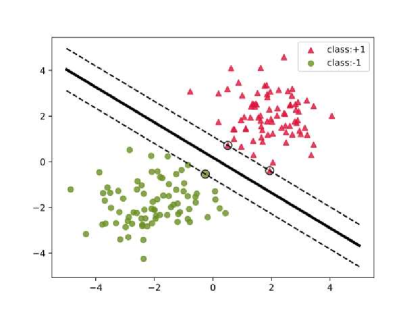
Figure 1: Decision hyperplane learned by hard-margin SVMs. Circles are support vectors.

The SVM problem is based on the core principle of achieving classification by reducing the error rate and optimizing the hyperplane with the highest margin. This is illustrated in Fig.1, where the solid line represents the classification hyperplane $f(x)=0$. SVM employs the kernel function $\phi(x_{i})$ to transform low-dimensional features into higher-dimensional features in order to address nonlinear situations. The kernel approach is used to directly calculate the inner product between high-dimensional features, eliminating the requirement for explicit computation of nonlinear feature mappings. Afterwards, linear classification is conducted in the feature space with a high number of dimensions. soft-margin SVM utilizing kernel techniques can be expressed in the following manner:

$$\mathop{\min}_{\mathbf{w}\in\mathbb{R}^{n}}F(\mathbf{w}) =\cfrac{1}{l}\sum\limits_{i=1}^{l}f(\mathbf{w},\theta)$$ (3)

$$=\cfrac{C}{2}\lVert\mathbf{w}\rVert^{2}+\cfrac{1}{l}\sum\limits_{i=1}^{l}l((x_{i},y_{i});\mathbf{w})$$

where $f(\mathbf{w},\theta_{i})=\cfrac{C}{2}\lVert\mathbf{w}\rVert^{2}+\text{max}(0,1-y_{i}(\mathbf{w^{T}}x_{i}))$, and $C>0$ is a hyperparameter.

Considering imbalanced datasets, the solution of SVM may appear overfitting. Standard SVMs tend to assign any sample that comes into the class-heavy side. Fig.2 illustrates the above situation. When the dashed line is used as the classification hyperplane, the error rate is as high as 4.53%. When the solid line is used (the solid line is learned through the method proposed in this paper), the error rate is reduced to 2.13%. This illustrates the importance of improving data imbalances.

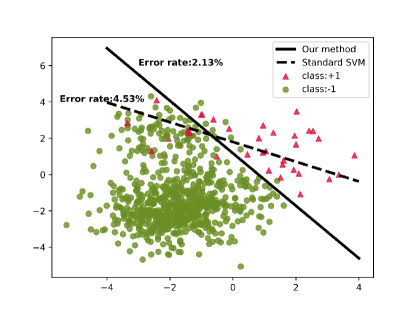
Figure 2: Decision hyperplane learned from imbalanced data. The solid line is the hyperplane obtained by the proposed method, while the dashed line is obtained by the standard solving algorithm.

In numerous real-world engineering scenarios, the training data frequently encounters noise or outliers, resulting in substantial deviations in the decision bounds of SVM. The outlier sensitivity problem of ordinary SVM algorithms refers to this phenomena. Fig.3 demonstrates the atypical susceptibility of SVM. In the absence of outliers in the training data, the SVM algorithm can identify the optimal hyperplane, shown by a solid line, that maximizes the margin between the two classes. If an outlier exists on the other side, the decision hyperplane, indicated by a dashed line, deviates considerably from the optimal selection. Consequently, the training procedure of a typical SVM is highly susceptible to outliers.

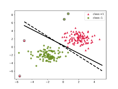
Figure 3: Decision hyperplane learned by hard-margin SVMs. The solid line is a decision hyperplane without noise, while the dashed line is a decision hyperplane with noise. The noises are marked as circles.

3.2 Soft-Margin Weighted Support Vector Machine (WSVM)

Soft-Margin Weighted Support Vector Machine (WSVM), aims to apply distinct weights to individual data points based on their relative significance within the class. This enables individual data points to exert varying influences on the decision hyperplane. Set $\alpha_{i}$ as the weight of the $ith$ a sample $x_{i}$, then the training data set into $\{(x_{i},y_{i},\alpha_{i})\}_{i=1}^{l}$, the $\alpha_{i}$ is continuous and $0\leq\alpha_{i}\leq 1$. Then the optimization problem can be written as:

$$\mathop{\min}_{\mathbf{w}\in\mathbb{R}^{n}}F(\mathbf{w}) =\dfrac{1}{l}\sum\limits_{i=1}^{l}f(\mathbf{w},\theta)$$ (4)

$$=\dfrac{C}{2l}\sum\limits_{i=1}^{l}\lVert\mathbf{w}\rVert^{2}+\dfrac{1}{l}\sum\limits_{i=1}^{l}l((x_{i},y_{i},\alpha_{i});\mathbf{w})$$

where $f(\mathbf{w},\theta_{i})=\frac{1}{2}\alpha_{i}C\lVert\mathbf{w}\rVert^{2}+\text{max}(0,1-y_{i}(\mathbf{w^{T}}x_{i}))$ We need to ensure that the objective function $F(\mathbf{w})$ is minimized when $\alpha_{i}$ is larger. Since the second term of the objective function is zero, it can only be that the $l_{2}$ norm of $\mathbf{w}$ tends to be smaller. It satisfies the spacing maximization principle.

Obviously, the standard SVM and the proposed WSVM are different in weight coefficient $\alpha_{i}$. The higher the value of $\alpha_{i}$, the more significant the sample’s contribution to the decision hyperplane. In conventional SVM, samples are considered equal, meaning that each sample has an equal impact on the decision hyperplane. However, that is not true. In the real datasets, there are imbalanced samples and outliers. The large number of samples and the presence of outliers will result in the decision hyperplane deviating, which is undesirable. Consequently, it is necessary to diminish or disregard the impact of these samples, while amplifying the significance of the limited categories of samples, support vectors, and accurately classified samples. This is what WSVM does. Both WSVM and SVM ensure maximum spacing, facilitating the differentiation between the two categories of data. Furthermore, the former also prioritizes the analysis of samples that have a greater impact.

3.3 Adaptive Weight Function(AW Function)

The weight of sample is developed based on the distance. Suppose that the distance between the sample and the hyperplane is d in the feature space, then $d$ obeys a Gaussian distribution with a mean value of 0. Its probability density function is

$$f(d)=\frac{1}{\sqrt{2\pi}\sigma}e^{-\frac{d^{2}}{2\sigma^{2}}}$$ (5)

The initial decision hyperplane $\mathbf{w_{0}}x+b=0$ is obtained. Set $d_{i}^{k}$ is the distance between the $i$ th sample and the initial decision hyperplane, in the $k$ th iteration, expression is as follows:

$$d_{i}^{k}=\frac{|\mathbf{w_{k}}x_{i}+b|}{\lVert\mathbf{w_{k}}\rVert},i=1,…,l$$ (6)

We stress the significance of the distance between the sample and the hyperplane. And according to the above assumption, we can give the definition of Adaptive Weight function(AW function).

Definition 1.

(AW function) In the $k$ th iteration, let $\alpha_{ki}$ be the weight of the $i$ th sample. Set $M=\text{max}\{d_{1}^{k},d_{2}^{k},…,d_{l}^{k}\},m=\text{min}\{d_{1}^{k},d_{2}^{k},…,d_{l}^{k}\}$. Accordingly, the following Adaptive Weight function(AW function) is proposed:

$$\alpha_{ki}=\frac{2}{\sqrt{2\pi}\sigma}e^{-\frac{(d_{i}^{k})^{2}}{2\sigma^{2}}}+\frac{1}{M-m}e^{-\frac{d_{i}^{k}}{M-m}}$$ (7)

where $M-m$ can weaken the influence of difference or variation amplitude on distribution to some extent.

According to different $\sigma$ values, we draw the AW function image, as shown in Fig.4. The function exhibits an axis of symmetry at $x=0$ and demonstrates a decreasing trend from the center toward the periphery. In the proposed framework, the x-axis indicates the spatial separation between the sample and the decision hyperplane, while the y-axis signifies the magnitude of the weight assigned to the sample. Therefore, the y-values should be in the range of 0 to 1. It is evident from this analysis that the value of $\sigma$ that yields the greatest match for our weight argument is 1.

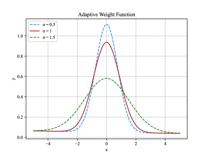
Figure 4: AW function with different $\sigma$ ($\sigma\in\{0.5,1,1.5\}$)

Demonstrate the reasonableness of the weighting function for the given set. The weight function should be expressed as a probability density function within each class, meaning that the integral value of the function is equal to 1 within each class. Furthermore, it is important to mention that, to enhance efficiency during the experiment, we will refrain from computing the distance based on the category. Hence, we do not differentiate between the two categories during the process of proof. In brief, we prove that the definite integral of the function equals 2.

Proof.

$$\int_{0}^{+\infty}\Bigg{(}\frac{2}{\sqrt{2\pi}\sigma}e^{-\frac{(d_{i}^{k})^{2}}{2\sigma^{2}}}+\frac{1}{M-m}e^{-\frac{d_{i}^{k}}{M-m}}\Bigg{)}d(d_{i}^{k})$$

$$=\int_{0}^{+\infty}\frac{2}{\sqrt{2\pi}\sigma}e^{-\frac{(d_{i}^{k})^{2}}{2\sigma^{2}}}d(d_{i}^{k})\\ +\int_{0}^{+\infty}\frac{1}{M-m}e^{-\frac{d_{i}^{k}}{M-m}}d(d_{i}^{k})$$

The first term is the probability density function of the Gaussian distribution, so

$$\int_{0}^{+\infty}\frac{2}{\sqrt{2\pi}\sigma}e^{-\frac{(d_{i}^{k})^{2}}{2\sigma^{2}}}d(d_{i}^{k})$$

$$=2\int_{0}^{+\infty}\frac{1}{\sqrt{2\pi}\sigma}e^{-\frac{(d_{i}^{k})^{2}}{2\sigma^{2}}}d(d_{i}^{k})$$

$$=\int_{-\infty}^{+\infty}\frac{1}{\sqrt{2\pi}\sigma}e^{-\frac{(d_{i}^{k})^{2}}{2\sigma^{2}}}d(d_{i}^{k})\\ =1$$

The second term is

$$\int_{0}^{+\infty}\frac{1}{M-m}e^{-\frac{d_{i}^{k}}{M-m}}d(d_{i}^{k})$$

$$=\frac{1}{M-m}\int_{0}^{+\infty}e^{-\frac{d_{i}^{k}}{M-m}}d(d_{i}^{k})$$

$$=\frac{1}{M-m}\big{(}-(M-m)e^{-\frac{d_{i}^{k}}{M-m}}\big{)}\big{|}_{0}^{+\infty}$$

$$=\frac{1}{M-m}(0+M-m)=1$$

So

$$\int_{0}^{+\infty}\Bigg{(}\frac{2}{\sqrt{2\pi}\sigma}e^{-\frac{(d_{i}^{k})^{2}}{2\sigma^{2}}}+\frac{1}{M-m}e^{-\frac{d_{i}^{k}}{M-m}}\Bigg{)}d(d_{i}^{k})=1+1=2$$

∎

For every category of samples, the weight function assigns a weight of 1 when the distance is 0. The weight diminishes proportionally with the distance. It fulfills the condition that samples close to the hyperplane have a greater impact.

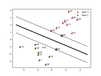
((a)) Weights of Different Samples

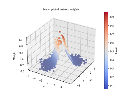
((b)) 3D Visualisation of Weights

Figure 5: Weights generated by AW function

3.4 Generalized Framework for AW-WSVM

On the basis of the theories in Sections 3.2 and 3.3, we give the most important contribution of this paper, a generalized framework named AW-WSVM. We apply this framework to standard stochastic optimization algorithms, such as Algorithm 1 and Algorithm 2, to solve WSVM and update the weights with AW function. The standard second-order algorithm oNAQ will be used in the following sections, so it is summarized in Algorithm 3.

Algorithm 3 oNAQ Method[39]

1:minibatch $X_{k}$, $0<\mu<1$, $k_{max}$, $\hat{H}_{k}=\epsilon I$ and $v_{k}=0$

2:$\mathbf{w}\in\mathbb{R}^{n}$

3:$k\leftarrow 1$

4:while $k<k_{max}$ do

5:     $\nabla F_{1}\leftarrow\nabla F(\mathbf{w_{k}}+\mu v_{k},X_{k})$

6:     $\hat{g}_{k}\leftarrow-\hat{H}_{k}\nabla F(\mathbf{w_{k}}+\mu v_{k},X_{k})$

7:     $\hat{g}_{k}=\frac{\hat{g}_{k}}{\lVert\hat{g}_{k}\rVert_{2}}$

8:     Determine $\alpha_{k}$ using

9:        $\alpha_{k}=\frac{\alpha_{0}}{\sqrt{k}}$

10:     $v_{k+1}\leftarrow\mu v_{k}+\alpha_{k}\hat{g}_{k}$

11:     $\mathbf{w_{k+1}}\leftarrow\mathbf{w_{k}}+v_{k+1}$

12:     $\nabla F_{2}\leftarrow\nabla F(\mathbf{w_{k+1}},X_{k})$

13:     $p_{k}\leftarrow\mathbf{w_{k+1}}-(\mathbf{w_{k}}+\mu v_{k})$

14:     $q_{k}\leftarrow\nabla F_{2}-\nabla F_{1}+\lambda p_{k}$

15:     Update $\hat{H}_{k}$ using

16:     

$$\hat{H}_{k+1}=\big{(}I-\frac{p_{k}q_{k}^{T}}{q_{k}^{T}p_{k}}\big{)}\hat{H}_{k}\big{(}I-\frac{q_{k}p_{k}^{T}}{q_{k}^{T}p_{k}}\big{)}+\frac{p_{k}p_{k}^{T}}{q_{k}^{T}p_{k}}$$

17:     $k\leftarrow k+1$

18:end while

All samples are initially assigned the same weight, i.e., $\alpha_{0i}=\frac{2}{l},i=1,...,l$, then $\sum\limits_{i=1}^{l}\alpha_{0i}=2$. The assumption in Section 3.3 is given to illustrate the rationality of the above statement.

Now, we can utilize the AW function mentioned before to produce weights for training the AW-WSVM algorithm. Enter the distance $d_{i}^{k}(i=1,2,...,l)$ obtained by the $kth$ training into the (7). Then update the weight of each sample $\alpha_{ki},i=1,...,l$. And then we put it in the objective function again. The framework includes the following steps:

(1) Solve the WSVM to get the hyperplane

Substitute the weight vector obtained from each update into formula (4), and get a new hyperplane expression through iterative solution of random optimization algorithm;

(2) Screen samples

We can calculate the distance (vector) between each sample and the hyperplane. Remember that the positive class sample set is $S_{+}$ and the negative class is $S_{-}$. If there is $x_{i}\in S_{+}$, so that the inner product of $x_{i}$ and $x_{j}$ (any $x_{j}\in S_{+}$) is less than or equal to 0, it means that $x_{i}$ is noise. We will eliminate it. In the same way, $S_{-}$ is also treated in this way;

(3) Update weights

Substitute the obtained sample distance into AW function, and get the weight of each sample.

Algorithm 4 Proposed AW-WSVM

1:The training set $(x_{i},y_{i},\alpha_{ki}),i=1,…,l$, the initial weight $\alpha_{0}=[\frac{2}{l},…,\frac{2}{l}]^{T}$, the original $\mathbf{w_{0}}=[0,…,0]^{T}$ and $k_{max}$.

2:$\mathbf{w}\in\mathbb{R}^{n}$

3:$k\leftarrow 1$

4:while $k<k_{max}$ do

5:     Obtain a solution $\mathbf{w_{k}}$ by Algorithm 3

6:     Calculate:

7:     $d_{i}^{k}=\frac{|\mathbf{w_{k}}x_{i}+b|}{\lVert\mathbf{w_{k}}\rVert},i=1,…,l$

8:     Eliminate noise

9:     set

$$M=\text{max}\{d_{1}^{k},d_{2}^{k},…,d_{l}^{k}\}$$

$$m=\text{min}\{d_{1}^{k},d_{2}^{k},…,d_{l}^{k}\}$$

10:     Update $\alpha_{k}=[\alpha_{k1},…,\alpha_{kl}]^{T}$

$$\alpha_{ki}=\frac{2}{\sqrt{2\pi}\sigma}e^{-\frac{(d_{i}^{k})^{2}}{2\sigma^{2}}}+\frac{1}{M-m}e^{-\frac{d_{i}^{k}}{M-m}}$$

11:     $k\leftarrow k+1$

12:end while

The hyperplane acquired at the $kth$ iteration is used as the beginning input for the $k+1$ iteration. The weight coefficient $\mathbf{w_{k+1}}$ and distance $d_{i}^{k+1}$ of the decision hyperplane are obtained again. Proceed with the aforementioned instructions to iterate. In this way, the outlier will have minimal weight, approaching zero, thereby greatly diminishing its impact on the choice hyperplane. Fig.5 displays the weights obtained for a certain class with the AW function. The data that was used for training points located in the middle region of the data group possess a substantially greater weight (close to 1), while the outliers have a much lower weight (close to 0). The proposed AW-WSVM is summarized in Algorithm 4.

4 Numerical Experiments

In this section, we present a comparison between the proposed method AW-WSVM and typical first-order and second-order approaches. The comparison is conducted on different datasets. We use experimental data to illustrate the effectiveness of the proposed framework in solving the problem of imbalanced data classification. These experiments were performed on python3 on MacOS with the Apple M2 chip.

To evaluate the proposed method comprehensively, it is insufficient to solely rely on a single indicator. Before providing the assessment criteria, it is necessary to establish the confusion matrix for the binary classifier. The confusion matrix provides fundamental details on the classifier’s actual and expected classifications (see Table 1). The discriminant criteria we offer include accuracy, precision, recall, sensitivity, specificity, and F1 score.
(1)Accuracy=$\frac{\text{TP+TN}}{\text{TP+TN+FN+FP}}$
(2)Precision=$\frac{\text{TP}}{\text{TP+FP}}$
(3)Recall=$\frac{\text{TP}}{\text{TP+FN}}$
(4)Specificity=$\frac{\text{TN}}{\text{TN+FP}}$
(5)Sensitivity=$\frac{\text{TP}}{\text{TP+FP}}$
(6)F1-score=$\frac{2\cdot\text{Recall}\cdot\text{Precision}}{\text{Recall+Precision}}$
(7)G-mean=$\sqrt{\text{Recall}\cdot\text{Specificity}}$

Table 1: Confusion matrix.

	Predicted positive	Predicted negative
True positive	TP	FN
True negative	FP	TN

4.1 Experiments on Different Datasets

In this section, to illustrate the universality of the proposed framework, we compare our proposed generalized framework, which combines standard first-order optimization algorithms SGD and second-order optimization algorithms oBFGS and oNAQ, with these algorithms on 12 real datasets. These datasets are diverse, including sparse, dense, imbalanced, high-dimensional, and low-dimensional. They were collected from the University of California, Irvine (UCI) Machine Learning repository, Libsvm data. Details of the features are shown in Table 2. The second column indicates the source of the data set, the third column indicates the quantity of data, the fourth column indicates the dimension, and the fifth column indicates the quantity of data categories. The proposed approach differs from the standard approach only in whether the weights are set and updated.

Table 2: The description of the different datasets.

Datasets	Source	Samples	Features	Classes
A7a	UCI	16100	123	2
A8a	UCI	22696	123	2
A9a	UCI	32561	123	2
Mushroom	UCI	8124	22	2
Yeast	UCI	892	8	2
Ijcnn1	DP01a	49990	22	2
W1a	JP98a	2477	300	2
W2a	JP98a	3470	300	2
W3a	JP98a	4912	300	2
W4a	JP98a	7366	300	2
W5a	JP98a	9888	300	2
W6a	JP98a	17188	300	2

In this section, the parameters are set as follows. The learning rate of SGD optimization algorithm on different data sets $\epsilon$ is selected from {0.1,0.3,0.5}; The parameter $\tau$ related to the learning rate $\epsilon_{t}$ in oBFGS optimization algorithm is set to 10, $\epsilon_{t}=\frac{\tau}{\tau+t}$($t$ represents the $t$ iteration). In addition, to ensure the stability of the value, the change value of the independent variable is introduced in the calculation of the step difference, where the difference coefficient of the independent variable $\gamma$ is set to 0.2 on all datasets. Parameters $\tau$ related to the learning rate $\epsilon_{t}$ in the oNAQ optimization algorithm are set to 10, momentum coefficient $\mu$ to 0.1, and difference coefficient of independent variable $\gamma$ to 0.2 on all data sets. The highest limit of iterations and batch size of all algorithms are selected based on the size of the datasets. Refer to Table 3 for a comprehensive explanation.

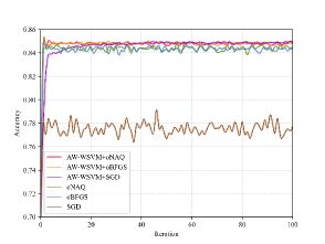
((a)) A7a

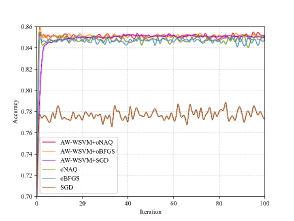
((b)) A8a

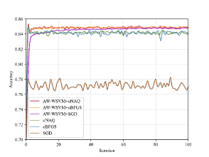
((c)) A9a

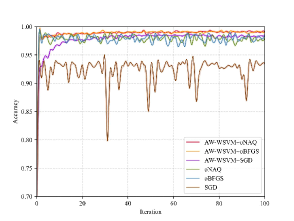
((d)) Mushroom

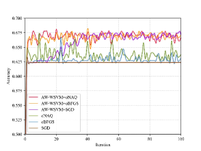
((e)) Yeast

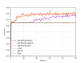
((f)) Ijcnn1

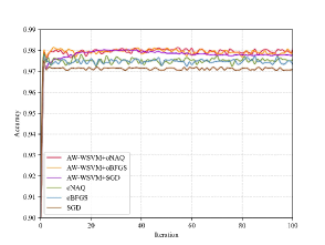
((g)) W1a

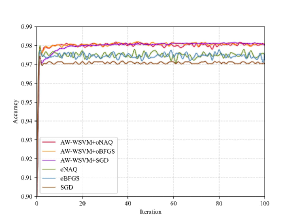
((h)) W2a

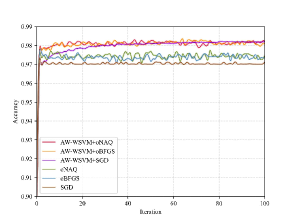
((i)) W3a

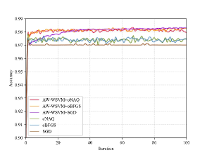
((j)) W4a

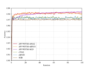
((k)) W5a

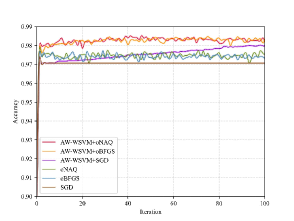
((l)) W6a

Figure 6: Comparison of accuracy between standard algorithms and AW-WSVM on real datasets ($\sigma$=1).

The variance $\sigma$ in the AW function is set to 1 empirically. We conducted 100 iterative experiments, taking the total amount of iterations as the horizontal coordinate and the test accuracy as the vertical coordinate to depict the performance of each algorithm, as shown in Fig.6. Fig.6(a)-6(c) respectively plotted the experimental results of the 12 datasets in Table 2. No matter whether the proposed method in the initial result performs well or not, it tends to be stable after a certain number of iterations. We can conclude that the proposed approach effectively improves the performance of SGD, oBFGS and oNAQ on all 12 datasets.

We additionally evaluate the efficacy of the proposed framework, AW-WSVM, by using the confusion matrix. To ensure the stability of the results, we iterated 100 times. The metrics of different algorithms obtained from the confusion matrix can be presented in Table 4-8, with the highest metrics bolded. Conclusions are easy to come by, and the proposed method outperforms SGD, oBFGS, and oNAQ on 11 datasets. The proposed method exhibits lower results with regard to accuracy, recall, sensitivity, and F1 scores when compared to oBFGS without weight involvement on the A7a dataset. However, when considering the entirety of the recommended technique, it has successfully attained the intended outcome.

Table 3: Details of parameter settings.

Datasets	SGD			oBFGS				oNAQ
	$\epsilon$	iter	Batchsize	$\tau$	$\gamma$	iter	Batchsize	$\tau$	$\mu$	$\gamma$	iter	Batchsize
A7a	0.1	50	256	10	0.2	100	128	10	0.1	0.2	100	128
A8a	0.1	100	32	10	0.2	100	128	10	0.1	0.2	100	128
A9a	0.1	50	256	10	0.2	100	128	10	0.1	0.2	100	128
Mushroom	0.1	50	256	10	0.2	100	64	10	0.1	0.2	100	64
Yeast	0.3	50	128	10	0.2	50	64	10	0.1	0.2	50	64
Ijcnn1	0.5	50	64	10	0.2	50	64	10	0.1	0.2	50	64
W1a	0.5	50	64	10	0.2	50	64	10	0.1	0.2	50	64
W2a	0.5	50	64	10	0.2	50	64	10	0.1	0.2	50	64
W3a	0.5	50	64	10	0.2	50	64	10	0.1	0.2	50	64
W4a	0.5	50	64	10	0.2	50	64	10	0.1	0.2	50	64
W5a	0.5	50	64	10	0.2	50	64	10	0.1	0.2	50	64
W6a	0.5	50	64	10	0.2	50	64	10	0.1	0.2	50	64

The findings presented in Table 4-8 indicate that, when considering a specific algorithm applied to the identical dataset, the recall rate, precision, sensitivity, and F1 score remain consistent. However, the prediction accuracy demonstrates improvement. Our model demonstrates a higher level of accuracy in identifying samples from each category throughout data processing. Put simply, the model exhibits enhanced generalization and stability, enabling it to effectively process data in real-world scenarios.

4.2 Statistical Comparison

This section makes a statistical comparison [40] of the experimental results. The significance of performance differences between classifiers, including test accuracy and prediction accuracy, were tested using Friedman tests and Nemenyi post hoc tests [41, 42]. The Friedman test is utilized to compare the mean ranking of several algorithms on N datasets. Define $r_{i}^{j}$ as the ranking of the $j$ th algorithm on the $i$ th dataset out of a total of N datasets, and $R_{j}=\frac{1}{N}\sum_{i=1}^{N}r_{i}^{j}$. According to the null hypothesis, all algorithms are considered to be identical, so their average ranking $R_{j}$ should be the same. The Friedman statistic $R_{j}$ follows a Chi-square distribution with K-1 degrees of freedom

$$\chi_{F}^{2}=\frac{12N}{K(K+1)}[R_{j}^{2}-\frac{(K(K+1)^{2})}{4}]$$ (8)

where $K$ is the number of algorithms involved in the comparison.

Table 5 shows the average ranking $R_{j}$ of the six classifiers in test accuracy. The p-value of Friedman’s test is $1.7122\times 10^{-9}$. The P-value is less than the threshold for significance level $\alpha=0.05$, indicating that the null assumption should be discarded. The above results show that there are great differences among all classification methods from a statistical point of view. We compared the accuracy of the six classifiers (see Table 9), with a p-value of $1.8302\times 10^{-8}$ for Friedman’s test, indicating significant differences among all classification methods.

Table 4: Accuracy of six methods on different datasets.

Datasets	oNAQ	AW-WSVM+oNAQ	oBFGS	AW-WSVM+oBFGS	SGD	AW-WSVM+SGD
A7a	0.8431	0.8486	0.8453	0.8469	0.7682	0.8486
A8a	0.8492	0.8514	0.8456	0.8521	0.7767	0.8513
A9a	0.8425	0.8445	0.8434	0.8469	0.7733	0.8500
Mushroom	0.9832	0.9906	0.9791	0.9865	0.7733	0.9869
Yeast	0.6452	0.6498	0.6475	0.6498	0.6495	0.6495
Ijcnn1	0.9050	0.9207	0.9050	0.9193	0.9050	0.9151
W1a	0.9765	0.9805	0.9747	0.9790	0.9706	0.9780
W2a	0.9752	0.9805	0.9734	0.9816	0.9704	0.9816
W3a	0.9747	0.9800	0.9745	0.9812	0.9702	0.9823
W4a	0.9731	0.9812	0.9723	0.9818	0.9702	0.9827
W5a	0.9730	0.9830	0.9750	0.9816	0.9699	0.9828
W6a	0.9755	0.9830	0.9733	0.9849	0.9707	0.9845

Consequently, to determine the classifiers that exhibit substantial differences, it is essential to perform a post-hoc test in order to further differentiate between the methods. Nemenyi post hoc test is selected in this paper. The Nemenyi test calculates the critical range of the difference in average order values

$$CD=q_{\alpha}\sqrt{\frac{K(K+1)}{6N}}$$ (9)

If the discrepancy among the mean rank measurements of the two distinct algorithms exceeds the critical range (CD), the hypothesis that the two algorithms exhibit comparable results is refuted with the equivalent level of confidence. The variables $K$ and $N$ correspond to the quantities of algorithms and datasets, correspondingly. When the significant level $\alpha$=0.05, $q_{\alpha}$=2.850. So we get CD = 2.85×$\sqrt{6(6+1)/(6\times 12)}$=2.1767.

Fig.7(a) and Fig.7(b) respectively report the analysis results of six classifiers in terms of test accuracy and precision. The test accuracy of the standard SGD, oBFGS, and oNAQ algorithms does not exhibit any substantial variation, but there is a notable disparity between the proposed approach in this research. Furthermore, our analysis indicates that the integration of all three algorithms with AW-WSVM leads to enhanced algorithm performance. This improvement is evident from the overall higher ranking of the combined algorithms across all datasets, showcasing varied progress. The results indicate a negligible disparity in the classification accuracy across standard SGD, oBFGS, and oNAQ. Each of the three algorithms was examined independently. The performance of SGD was enhanced by using the weight update approach suggested in this research (AW-WSVM+SGD). Notably, there were notable disparities between the two algorithms when compared to the original SGD. The same applies to second-order approaches such as BFGS and NAQ.

Table 5: Precision of six methods on different datasets.

Datasets	oNAQ	AW-WSVM+oNAQ	oBFGS	AW-WSVM+oBFGS	SGD	AW-WSVM+SGD
A7a	0.8201	0.8216	0.8212	0.8200	0.7667	0.8486
A8a	0.8250	0.8250	0.8219	0.8275	0.7735	0.8282
A9a	0.8206	0.8216	0.8181	0.8222	0.7710	0.8258
Mushroom	0.9651	0.9798	0.9564	0.9714	0.7585	0.9725
Yeast	0.6241	0.6285	0.6277	0.6293	0.6004	0.6004
Ijcnn1	0.9050	0.9180	0.9050	0.9169	0.9050	0.9133
W1a	0.9763	0.9802	0.9747	0.9787	0.9706	0.9777
W2a	0.9750	0.9802	0.9733	0.9813	0.9704	0.9813
W3a	0.9746	0.9788	0.9744	0.9809	0.9702	0.9820
W4a	0.9730	0.9809	0.9722	0.9815	0.9702	0.9824
W5a	0.9729	0.9827	0.9749	0.9813	0.9699	0.9825
W6a	0.9753	0.9827	0.9732	0.9847	0.9707	0.9842

Table 6: Recall of six methods on different datasets.

Datasets	oNAQ	AW-WSVM+oNAQ	oBFGS	AW-WSVM+oBFGS	SGD	AW-WSVM+SGD
A7a	0.8201	0.8216	0.8212	0.8200	0.7667	0.8486
A8a	0.8250	0.8250	0.8219	0.8275	0.7735	0.8282
A9a	0.8206	0.8216	0.8181	0.8222	0.7710	0.8258
Mushroom	0.9651	0.9798	0.9564	0.9714	0.7585	0.9725
Yeast	0.6241	0.6285	0.6277	0.6293	0.6004	0.6004
Ijcnn1	0.9050	0.9180	0.9050	0.9169	0.9050	0.9133
W1a	0.9763	0.9802	0.9747	0.9787	0.9706	0.9777
W2a	0.9750	0.9802	0.9733	0.9813	0.9704	0.9813
W3a	0.9746	0.9788	0.9744	0.9809	0.9702	0.9820
W4a	0.9730	0.9809	0.9722	0.9815	0.9702	0.9824
W5a	0.9729	0.9827	0.9749	0.9813	0.9699	0.9825
W6a	0.9753	0.9827	0.9732	0.9847	0.9707	0.9842

Table 7: Sensitivity of six methods on different datasets.

Datasets	oNAQ	AW-WSVM+oNAQ	oBFGS	AW-WSVM+oBFGS	SGD	AW-WSVM+SGD
A7a	0.8201	0.8216	0.8212	0.8200	0.7667	0.8486
A8a	0.8250	0.8250	0.8219	0.8275	0.7735	0.8282
A9a	0.8206	0.8216	0.8181	0.8222	0.7710	0.8258
Mushroom	0.9651	0.9798	0.9564	0.9714	0.7585	0.9725
Yeast	0.6241	0.6285	0.6277	0.6293	0.6004	0.6004
Ijcnn1	0.9050	0.9180	0.9050	0.9169	0.9050	0.9133
W1a	0.9763	0.9802	0.9747	0.9787	0.9706	0.9777
W2a	0.9750	0.9802	0.9733	0.9813	0.9704	0.9813
W3a	0.9746	0.9788	0.9744	0.9809	0.9702	0.9820
W4a	0.9730	0.9809	0.9722	0.9815	0.9702	0.9824
W5a	0.9729	0.9827	0.9749	0.9813	0.9699	0.9825
W6a	0.9753	0.9827	0.9732	0.9847	0.9707	0.9842

Table 8: F1-score of six methods on different datasets.

Datasets	oNAQ	AW-WSVM+oNAQ	oBFGS	AW-WSVM+oBFGS	SGD	AW-WSVM+SGD
A7a	0.8201	0.8216	0.8212	0.8200	0.7667	0.8486
A8a	0.8250	0.8250	0.8219	0.8275	0.7735	0.8282
A9a	0.8206	0.8216	0.8181	0.8222	0.7710	0.8258
Mushroom	0.9651	0.9798	0.9564	0.9714	0.7585	0.9725
Yeast	0.6241	0.6285	0.6277	0.6293	0.6004	0.6004
Ijcnn1	0.9050	0.9180	0.9050	0.9169	0.9050	0.9133
W1a	0.9763	0.9802	0.9747	0.9787	0.9706	0.9777
W2a	0.9750	0.9802	0.9733	0.9813	0.9704	0.9813
W3a	0.9746	0.9788	0.9744	0.9809	0.9702	0.9820
W4a	0.9730	0.9809	0.9722	0.9815	0.9702	0.9824
W5a	0.9729	0.9827	0.9749	0.9813	0.9699	0.9825
W6a	0.9753	0.9827	0.9732	0.9847	0.9707	0.9842

Table 9: Friedman ranking of these methods according to prediction accuracies on different datasets.

Datasets	oNAQ	AW-WSVM+oNAQ	oBFGS	AW-WSVM+oBFGS	SGD	AW-WSVM+SGD
A7a	4	1.5	3	2	5	1.5
A8a	4	2	5	1	6	3
A9a	4	2	5	1	6	3
Mushroom	4	1	5	3	6	2
Yeast	4	1.5	3	1.5	2.5	2.5
Ijcnn1	4.5	1	4.5	2	4.5	3
W1a	4	1	5	2	6	3
W2a	3	2	4	1.5	5	1.5
W3a	4	3	5	2	6	1
W4a	4	3	5	2	6	1
W5a	5	1	4	3	6	2
W6a	4	3	5	1	6	2
R	4.04	1.83	4.46	1.83	5.42	2.13

Table 10: Friedman ranking of these methods according to precisions on different datasets.

Datasets	oNAQ	AW-WSVM+oNAQ	oBFGS	AW-WSVM+oBFGS	SGD	AW-WSVM+SGD
A7a	4	2	3	5	6	1
A8a	3.5	3.5	4	2	5	1
A9a	4	2	5	1	6	3
Mushroom	4	1	5	3	6	2
Yeast	4	2	3	1	5.5	5.5
Ijcnn1	4.5	1	4.5	2	4.5	3
W1a	4	1	5	2	6	3
W2a	3	2	4	1.5	5	1.5
W3a	4	3	5	2	6	1
W4a	4	3	5	2	6	1
W5a	5	1	4	3	6	2
W6a	4	3	5	1	6	2
R	4	2.04	4.38	2.13	5.67	2.17

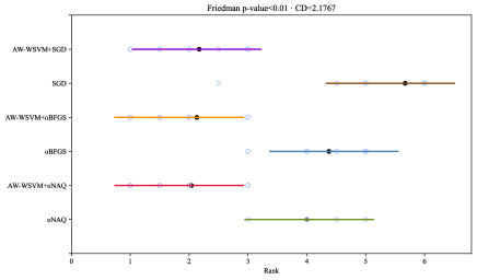
((a)) Classification accuracy

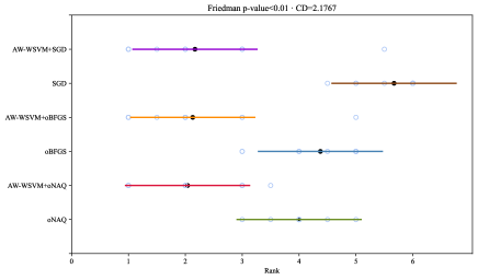
((b)) Classification precision

Figure 7: Comparison of all classifiers against each other with the Nemenyi post-hoc test.

4.3 Experiments on Emotional Classification with Different Imbalance Ratio(IR)

In this section, we collect the dataset of emotion classification, which comes from gitte (see Tabel 11). The last column in the table indicates the imbalance ratio (IR). In daily life, different kinds of news data are always imbalanced, for example, entertainment news will account for more than science and technology news.

In this section, the parameters are set as follows. The learning rate $\epsilon$ of SGD optimization algorithm is 0.1. The parameter $\tau$ in oBFGS and oNAQ optimization algorithm is set to 10 and $\gamma$ is set to 0.2. The momentum coefficient $\mu$ to 0.1. The highest limit of iterations is set to 500 and batchsize of all algorithms is set to 256.

Table 12 and Table 13 record the test accuracy and G-means after 100 iterations, respectively, in which bold indicates the best results compared with the two. It is well known that G-means can be used as an effective indicator to measure the quality of the model when the data is unbalanced. Therefore, we can draw the conclusion that our framework, AW-WSVM, will effectively improve the performance of the standard stochastic optimization algorithm, no matter whether the IR is high or low.

In order to further illustrate the effectiveness of the proposed AW-WSVM framework, we process the same data and get G-means under different IRs[43]. In order to further illustrate the effectiveness of the proposed AW-WSVM framework, we process the same data and get G-means under different IR. Taking 102vs100 as an example, we plot the results in Fig8. It is not difficult to find that our proposed method performs best in both low IR and high IR.

Table 11: The description of the emotional datasets.

Datasets	Samples	Features	Classes	IR
102_vs_100	45669	12	2	6.28
109_vs_116	70843	12	2	1.42
109_vs_100	47816	12	2	6.62
107_vs_106	53457	12	2	2.02
103_vs_115	56890	12	2	1.94
101_vs_100	34304	12	2	4.47

Table 12: Accuracy of different methods on emotional datasets.

Datasets	oNAQ	AW-WSVM+oNAQ	oBFGS	AW-WSVM+oBFGS	SGD	AW-WSVM+SGD
102_vs_100	0.9541	0.9558	0.9533	0.9564	0.9465	0.9580
109_vs_116	0.9125	0.9189	0.9123	0.9197	0.9058	0.9186
109_vs_100	0.9895	0.9902	0.9902	0.9907	0.9894	0.9899
107_vs_106	0.9700	0.9734	0.9703	0.9737	0.9664	0.9724
103_vs_115	0.9825	0.9832	0.9819	0.9833	0.9822	0.9832
101_vs_100	0.9721	0.9735	0.9726	0.9733	0.9708	0.9730

Table 13: G-mean of different methods on emotional datasets.

Datasets	oNAQ	AW-WSVM+oNAQ	oBFGS	AW-WSVM+oBFGS	SGD	AW-WSVM+SGD
102_vs_100	0.8203	0.8260	0.8169	0.8278	0.7817	0.8353
109_vs_116	0.8340	0.8454	0.8335	0.8468	0.8228	0.8447
109_vs_100	0.9533	0.9561	0.9563	0.9585	0.9530	0.9550
107_vs_106	0.9346	0.9417	0.9352	0.9424	0.9274	0.9397
103_vs_115	0.9620	0.9635	0.9607	0.9636	0.9613	0.9634
101_vs_100	0.9136	0.9147	0.9117	0.9143	0.9063	0.9121

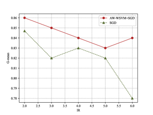
((a))

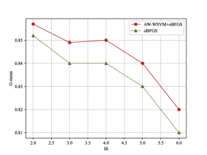
((b))

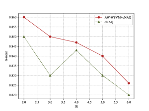
((c))

Figure 8: Comparisons on different IRs.

5 Conclusion

We proposes a novel generalized framework, referred to as AW-WSVM, for SVM. The purpose of its development was to address the complexities of real-world applications by effectively handling uncertain information. It ensures that training remains effective even when dealing with challenging and extensive datasets, without compromising on speed.

Considering massive amounts of data, the measurement of the distance between the samples and the decision hyperplane can be calculated with a Gaussian distribution. Therefore, the weights of the samples can be updated by the Adaptive weight function (AW function). Our analysis demonstrates that the weights generated by the AW function obey a probability distribution in each class. Unconstrained soft interval support vector machines have been improved through the addition of weighting coefficients, aligning with the fundamental concept. Subsequently, we can allocate greater weights to samples that are in close proximity to the decision hyperplane, while assigning lower weights to the other samples. Our allocation technique is appropriate since the support vectors, which are placed near the decision hyperplane, correspond with the concept that samples close to the decision plane have higher influence.

The proposed framework, AW-WSVM, was evaluated on a total of 12 datasets sourced from UCI repositories, LIBSVM repositories, and emotional datasets. The experiments conducted confirm that the proposed framework AW-WSVM surpasses the conventional first-order approaches SGD, second-order methods oBFGS, and oNAQ. Furthermore, it exhibited superior performance in terms of classification accuracy, precision, recall, sensitivity, and F1 score. In addition, we also conducted statistical experiments on these six classifiers. Friedman tests and Nemenyi post hoc tests demonstrate that the standard algorithms SGD, oBFGS, and oNAQ all perform better within our proposed framework. We not only do experiments on standard datasets, but also apply the framework to emotion classification datasets. From the G-means and other indicators, the framework proposed in this paper can effectively improve the performance of standard optimization algorithms, no matter whether the imbalance index is high or low. Moreover, the core of the proposed generalized framework, AW-WSVM, is to look for data samples near the classified hyperplane. Consequently, it may be effectively integrated with any soft-margin SVM solution techniques.

Declaration of Generative AI and AI-assisted technologies in the writing process

During the preparation of this work, the authors used ChatGPT in order to translate and revise some parts of the paper. After using this tool, the authors reviewed and edited the content as needed and took full responsibility for the content of the publication.

References

- [1] Vladimir Vapnik. The nature of statistical learning theory. Springer science & business media, 1999.
- [2] Yu-Xin Li, Yuan-Hai Shao, and Nai-Yang Deng. Improved prediction of palmitoylation sites using pwms and svm. Protein and peptide letters, 18(2):186–193, 2011.
- [3] Dino Isa, Lam H Lee, VP Kallimani, and Rajprasad Rajkumar. Text document preprocessing with the bayes formula for classification using the support vector machine. IEEE Transactions on Knowledge and Data engineering, 20(9):1264–1272, 2008.
- [4] Yingjie Tian, Yong Shi, and Xiaohui Liu. Recent advances on support vector machines research. Technological and economic development of Economy, 18(1):5–33, 2012.
- [5] Irene Kotsia, Weiwei Guo, and Ioannis Patras. Higher rank support tensor machines for visual recognition. Pattern Recognition, 45(12):4192–4203, 2012.
- [6] Aditya Tayal, Thomas F Coleman, and Yuying Li. Primal explicit max margin feature selection for nonlinear support vector machines. Pattern recognition, 47(6):2153–2164, 2014.
- [7] Dehua Liu, Hui Qian, Guang Dai, and Zhihua Zhang. An iterative svm approach to feature selection and classification in high-dimensional datasets. Pattern Recognition, 46(9):2531–2537, 2013.
- [8] Yonggan Wu, Bo Wei, Haizhou Liu, Tianxian Li, and Simon Rayner. Mirpara: a svm-based software tool for prediction of most probable microrna coding regions in genome scale sequences. BMC bioinformatics, 12(1):1–14, 2011.
- [9] Huaxiang Zhang, Linlin Cao, and Shuang Gao. A locality correlation preserving support vector machine. Pattern Recognition, 47(9):3168–3178, 2014.
- [10] Tao Xiong and Vladimir Cherkassky. A combined svm and lda approach for classification. In Proceedings. 2005 IEEE International Joint Conference on Neural Networks, 2005., volume 3, pages 1455–1459. IEEE, 2005.
- [11] Subhransu Maji, Alexander C Berg, and Jitendra Malik. Efficient classification for additive kernel svms. IEEE transactions on pattern analysis and machine intelligence, 35(1):66–77, 2012.
- [12] Thorsten Joachims, Thomas Finley, and Chun-Nam John Yu. Cutting-plane training of structural svms. Machine learning, 77:27–59, 2009.
- [13] Cho-Jui Hsieh, Kai-Wei Chang, Chih-Jen Lin, S Sathiya Keerthi, and Sellamanickam Sundararajan. A dual coordinate descent method for large-scale linear svm. In Proceedings of the 25th international conference on Machine learning, pages 408–415, 2008.
- [14] Fa Zhu, Jian Yang, Ning Ye, Cong Gao, Guobao Li, and Tongmin Yin. Neighbors’ distribution property and sample reduction for support vector machines. Applied Soft Computing, 16:201–209, 2014.
- [15] Bernhard E Boser, Isabelle M Guyon, and Vladimir N Vapnik. A training algorithm for optimal margin classifiers. In Proceedings of the fifth annual workshop on Computational learning theory, pages 144–152, 1992.
- [16] Xuegong Zhang. Using class-center vectors to build support vector machines. In Neural Networks for Signal Processing IX: Proceedings of the 1999 IEEE Signal Processing Society Workshop (Cat. No. 98TH8468), pages 3–11. IEEE, 1999.
- [17] Léon Bottou and Yann Cun. Large scale online learning. Advances in neural information processing systems, 16, 2003.
- [18] Léon Bottou. Large-scale machine learning with stochastic gradient descent. In Proceedings of COMPSTAT’2010: 19th International Conference on Computational StatisticsParis France, August 22-27, 2010 Keynote, Invited and Contributed Papers, pages 177–186. Springer, 2010.
- [19] Rehan Akbani, Stephen Kwek, and Nathalie Japkowicz. Applying support vector machines to imbalanced datasets. In Machine Learning: ECML 2004: 15th European Conference on Machine Learning, Pisa, Italy, September 20-24, 2004. Proceedings 15, pages 39–50. Springer, 2004.
- [20] Dacheng Tao, Xiaoou Tang, Xuelong Li, and Xindong Wu. Asymmetric bagging and random subspace for support vector machines-based relevance feedback in image retrieval. IEEE transactions on pattern analysis and machine intelligence, 28(7):1088–1099, 2006.
- [21] Chun-Fu Lin and Sheng-De Wang. Fuzzy support vector machines. IEEE transactions on neural networks, 13(2):464–471, 2002.
- [22] Yuan-Hai Shao, Wei-Jie Chen, Jing-Jing Zhang, Zhen Wang, and Nai-Yang Deng. An efficient weighted lagrangian twin support vector machine for imbalanced data classification. Pattern Recognition, 47(9):3158–3167, 2014.
- [23] Qi Fan, Zhe Wang, Dongdong Li, Daqi Gao, and Hongyuan Zha. Entropy-based fuzzy support vector machine for imbalanced datasets. Knowledge-Based Systems, 115:87–99, 2017.
- [24] Qi Kang, Lei Shi, MengChu Zhou, XueSong Wang, QiDi Wu, and Zhi Wei. A distance-based weighted undersampling scheme for support vector machines and its application to imbalanced classification. IEEE transactions on neural networks and learning systems, 29(9):4152–4165, 2017.
- [25] Xulei Yang, Qing Song, and Aize Cao. Weighted support vector machine for data classification. In Proceedings. 2005 IEEE International Joint Conference on Neural Networks, 2005., volume 2, pages 859–864. IEEE, 2005.
- [26] Xiaoyun Wu and Rohini Srihari. Incorporating prior knowledge with weighted margin support vector machines. In Proceedings of the tenth ACM SIGKDD international conference on Knowledge discovery and data mining, pages 326–333, 2004.
- [27] Li Zhang and Wei-Da Zhou. Density-induced margin support vector machines. Pattern Recognition, 44(7):1448–1460, 2011.
- [28] Mohammad Javad Abdi, Seyed Mohammad Hosseini, Mansoor Rezghi, et al. A novel weighted support vector machine based on particle swarm optimization for gene selection and tumor classification. Computational and mathematical methods in medicine, 2012, 2012.
- [29] Wei Du, Zhongbo Cao, Tianci Song, Ying Li, and Yanchun Liang. A feature selection method based on multiple kernel learning with expression profiles of different types. BioData mining, 10(1):1–16, 2017.
- [30] Fa Zhu, Jian Yang, Junbin Gao, and Chunyan Xu. Extended nearest neighbor chain induced instance-weights for svms. Pattern Recognition, 60:863–874, 2016.
- [31] Somaye Moslemnejad and Javad Hamidzadeh. Weighted support vector machine using fuzzy rough set theory. Soft Computing, 25(13):8461–8481, 2021.
- [32] Herbert Robbins and Sutton Monro. A stochastic approximation method. The annals of mathematical statistics, pages 400–407, 1951.
- [33] John Duchi, Elad Hazan, and Yoram Singer. Adaptive subgradient methods for online learning and stochastic optimization. Journal of machine learning research, 12(7), 2011.
- [34] Geoffrey Hinton, N Srivastava, K Swersky, T Tieleman, and A Mohamed. Coursera: Neural networks for machine learning. Lecture 9c: Using noise as a regularizer, 2012.
- [35] Diederik P Kingma and Jimmy Ba. Adam: A method for stochastic optimization. arXiv preprint arXiv:1412.6980, 2014.
- [36] Nicol N Schraudolph, Jin Yu, and Simon Günter. A stochastic quasi-newton method for online convex optimization. In Artificial intelligence and statistics, pages 436–443. PMLR, 2007.
- [37] Aryan Mokhtari and Alejandro Ribeiro. Global convergence of online limited memory bfgs. The Journal of Machine Learning Research, 16(1):3151–3181, 2015.
- [38] Richard H Byrd, Samantha L Hansen, Jorge Nocedal, and Yoram Singer. A stochastic quasi-newton method for large-scale optimization. SIAM Journal on Optimization, 26(2):1008–1031, 2016.
- [39] S Indrapriyadarsini, Shahrzad Mahboubi, Hiroshi Ninomiya, and Hideki Asai. A stochastic quasi-newton method with nesterov’s accelerated gradient. In Machine Learning and Knowledge Discovery in Databases: European Conference, ECML PKDD 2019, Würzburg, Germany, September 16–20, 2019, Proceedings, Part I, pages 743–760. Springer, 2020.
- [40] Huajun Wang, Weijun Zhou, and Yuanhai Shao. A new fast admm for kernelless svm classifier with truncated fraction loss. Knowledge-Based Systems, 283:111214, 2024.
- [41] Janez Demšar. Statistical comparisons of classifiers over multiple data sets. The Journal of Machine learning research, 7:1–30, 2006.
- [42] Romi Satria Wahono, Nanna Suryana Herman, and Sabrina Ahmad. A comparison framework of classification models for software defect prediction. Advanced Science Letters, 20(10-11):1945–1950, 2014.
- [43] Wanting Cai, Mingjie Cai, Qingguo Li, and Qiong Liu. Three-way imbalanced learning based on fuzzy twin svm. Applied Soft Computing, 150:111066, 2024.