Modeling of 2D self-drifting flame-balls in Hele-Shaw cells

On disintegration of lean hydrogen flames in narrow gaps

Abstract

The disintegration of near limit flames propagating through the gap of Hele-Shaw cells has recently become a subject of active research. In this paper, the flamelets resulting from the disintegration of the continuous front are interpreted in terms of the Zeldovich flame-balls stabilized by volumetric heat losses. A complicated free-boundary problem for 2D self-drifting near circular flamelets is reduced to a 1D model. The 1D formulation is then utilized to obtain the locus of the flamelet velocity, size, heat losses and Lewis numbers at which the self-drifting flamelets may exist.

Keywords Hydrogen flames  $\cdot$ Diffusive-thermal instability  $\cdot$ Flame-balls

1 Introduction

Hydrogen flames have gained increasing attention over the last years as a clean and efficient energy solution [1]. Apart from their technological relevance, hydrogen flames are remarkably rich dynamically. Because of the high diffusion coefficient of molecular hydrogen, lean hydrogen-air flames are known to experience diffusive-thermal instability [2,3] manifesting themselves in the formation of a cellular structure in a state of chaotic self-motion. Moreover, as has recently been discovered by Veiga-López et al. [4], lean hydrogen-air flames evolving in narrow gaps of Hele-Shaw chambers, and where heat-loss effects become important, continuous cellular flames may disintegrate forming self-drifting cup-like flamelets leaving tree-like or sprout-like traces (Fig. 1).

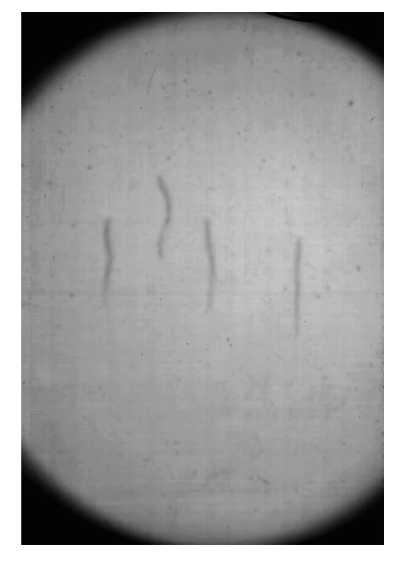
(a)

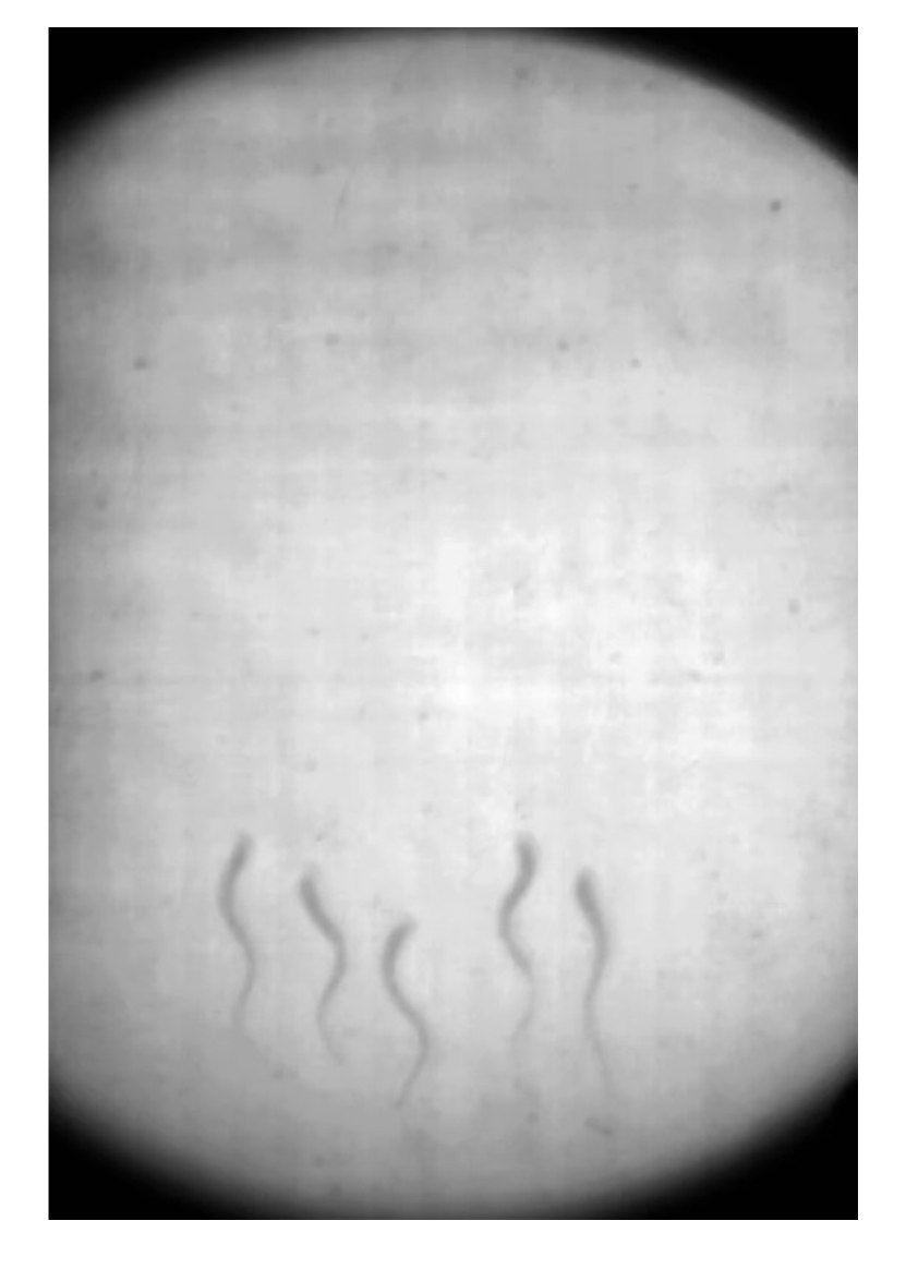
(b)

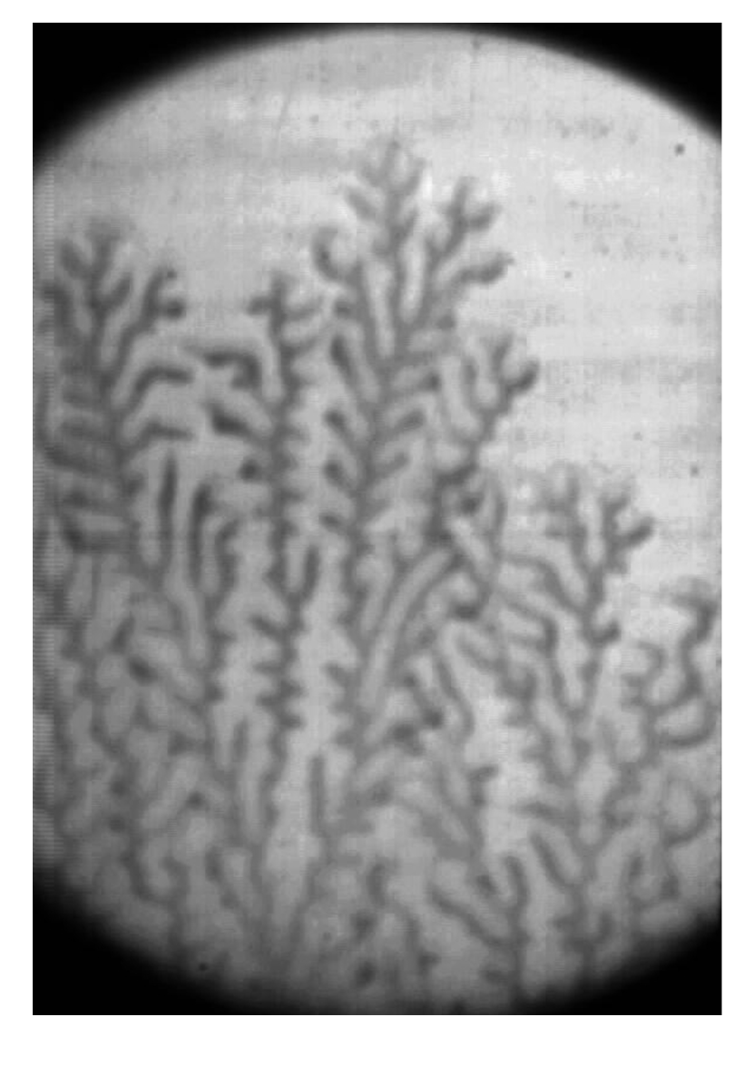
(c)

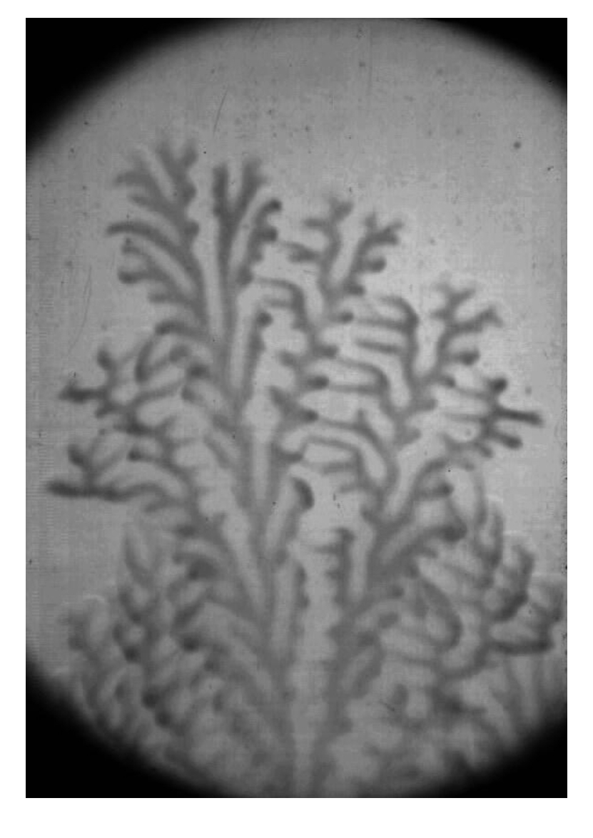
(d)

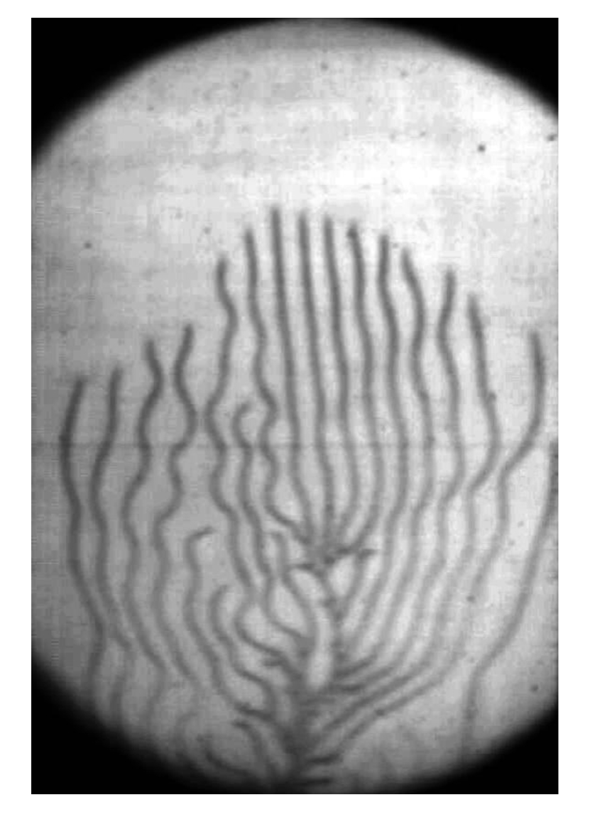
(e)

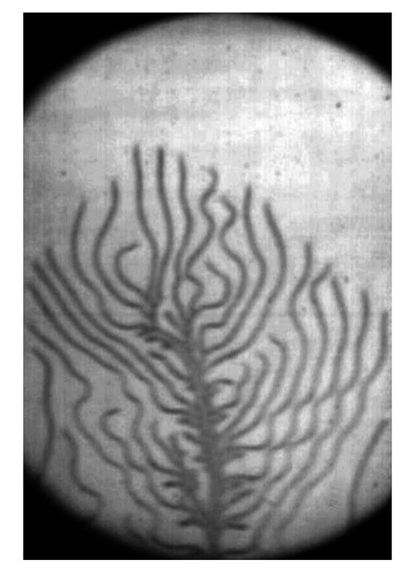
(f)

Figure 1: Hydrogen-air flamelets propagating through narrow gaps: (a) $d=5mm$, $\%H_{2}=5.0$; (b) $d=3mm$, $\%H_{2}=7.5$; (c) $d=4mm$, $\%H_{2}=7.0$; (d) $d=5mm$, $\%H_{2}=6.0$; (e) $d=2mm$, $\%H_{2}=9.75$; (f) $d=2mm$, $\%H_{2}=9.75$. Regimes: (a)(b) one-headed finger, (c)(d)(e)(f) one-headed branching.

These unexpected propagation modes extend flammability limits beyond those of the planar flames. This is particularly important for the safety studies of hydrogen-powered devices [5] as it implies that hydrogen flames may propagate in gaps much narrower than initially anticipated.

2 Reaction-diffusion model

Some of the above features of the Hele-Shaw flames may be successfully captured by an ultra-simple constant-density, buoyancy-free, reaction-diffusion model [6]. In suitably scaled variables and parameters it reads,

$$\dfrac{\partial T}{\partial t}=\dfrac{\partial^{2}T}{\partial x^{2}}+\dfrac{\partial^{2}T}{\partial y^{2}}+(1-\sigma)\Omega-q(T-\sigma),$$ (1)

$$\dfrac{\partial C}{\partial t}=\dfrac{1}{Le}\left(\dfrac{\partial^{2}C}{\partial x^{2}}+\dfrac{\partial^{2}C}{\partial y^{2}}\right)-\Omega,$$ (2)

$$\Omega=\dfrac{1}{2Le}(1-\sigma)^{2}N^{2}C\exp{\left[N\left(1-\dfrac{1}{T}\right)\right]},$$ (3)

where $T=$ temperature in units of $T_{b}$, the adiabatic temperature of combustion products; $C=$ concentration of the deficient reactant in units of $C_{0}$, its value in the fresh mixture; $x,y,t=$ spatio-temporal coordinates in units of $\ell_{th}=D_{th}/U_{b}$ and $\ell_{th}/U_{b}$, respectively; $\ell_{th}=$ thermal width of the flame; $U_{b}=$ speed of a planar adiabatic flame; $D_{th}=$ thermal diffusivity of the mixture, $\sigma=T_{0}/T_{b}$, where $T_{0}=$ temperature sustained at the walls of the Hele-Shaw cell; $Le=D_{th}/D_{mol}$ is the Lewis number; $D_{mol}=$ molecular diffusivity of the deficient reactant; $N=T_{a}/T_{b}=$ scaled activation energy; $T_{a}=$ activation temperature; $\Omega=$ appropriately normalized reaction rate to ensure that at large $N$ the scaled speed of the planar adiabatic flame is close to unity; $q=$ scaled heat loss intensity specified as $(\pi\ell_{th}/d)^{2}$; $d=$ width of the Hele-shaw cell. The adopted expression for $q$ stems from the 1D heat equation, $T_{t}=T_{zz}$, considered over the Hele-Shaw gap and subjected to isothermal boundary conditions, $T(z=\pm d/2\ell_{th},t)=\sigma$. Hence, $T-\sigma\sim\exp{\left[-\left(\pi\ell_{th}/d\right)^{2}t\right]}\cos{\left[\left(\pi\ell_{th}/d\right)z\right]}$. The exponential rate of the temperature decay is then extrapolated over the quasi-2D formulation of (1)-(2) in the $(x,y)$ plane.

Figures 2 and 3 display the results of numerical simulations of the effect of heat losses on the breaking up of the flame in 2D. The problem has also been explored by Martínez-Ruiz et al. [7] and Dejoan [8] through large-scale numerical simulations of a model accounting both for the gas thermal expansion, buoyancy and momentum loss.

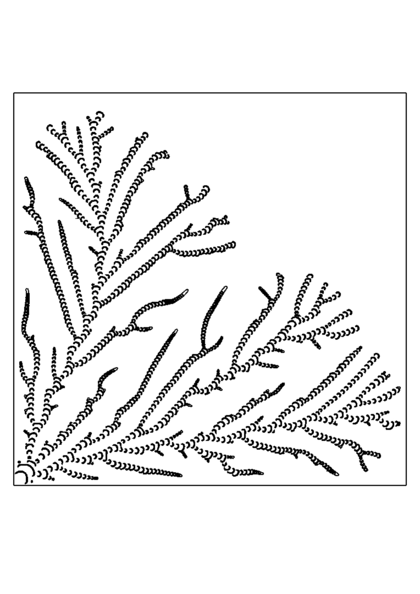
(a)

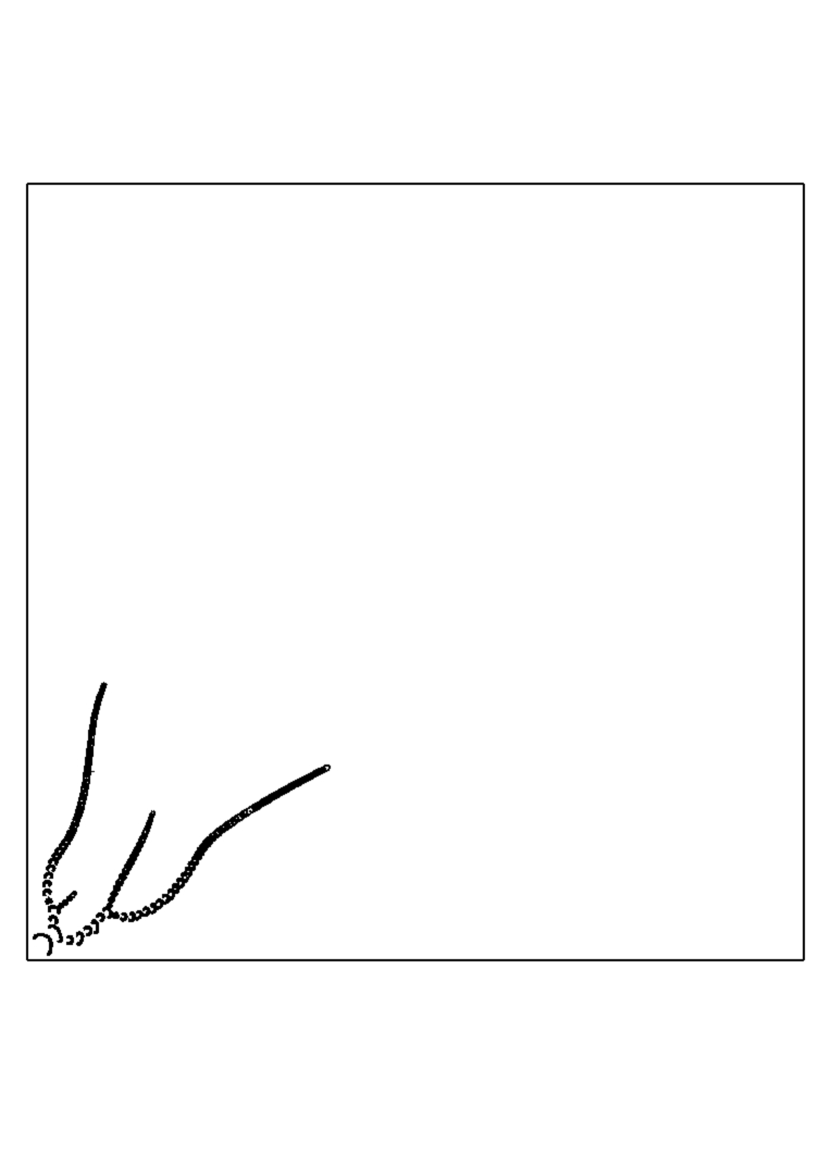
(b)

Figure 2: Reaction rate $\Omega=0.4$ at consecutive equispaced instants for one-headed flamelets under heat losses. Simulation of the reactive-diffusive system (1)-(3) for $N=10$; $Le=0.25$; $\sigma=0.2$; $q=0.14$, $0<t<740$ (a); $q=0.20$, $0<t<1000$ (b); $0<x,y<480$. Initial conditions, $T(x,y,0)=\sigma+(1-\sigma)\exp{[-(x^{2}+y^{2})/\ell^{2}]}$, $\ell=0.25$, $C(x,y,0)=1$, and adiabatic boundary conditions.

(a)

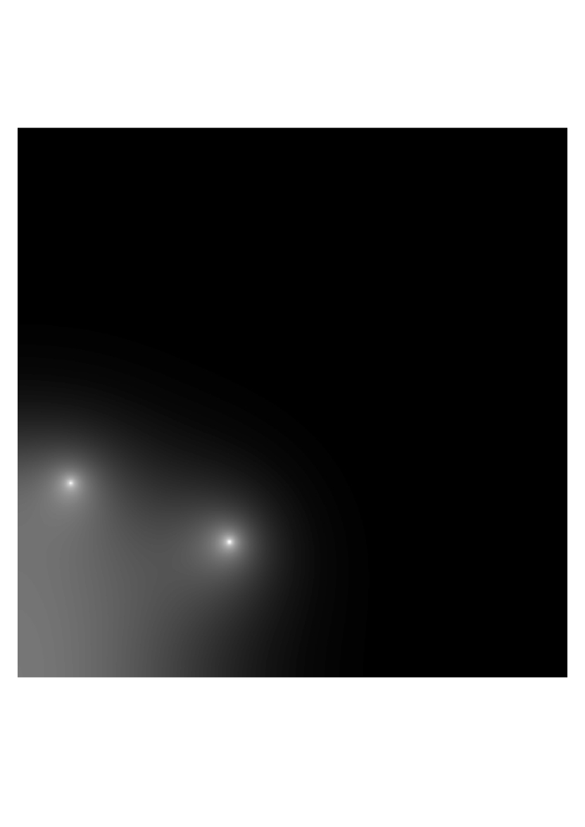
(b)

Figure 3: Distribution of the deficient reactant concentration, $C$, at $t=740$ (a) and $t=1000$ (b). For conditions see the legend for Fig.2. Lighter shading corresponds to lower concentration.

Near the quenching point, $q=0.22$, higher heat losses lead to a smaller drift velocity and flamelet size (Fig. 2), which is in line with experimental findings (Figs. 4, 5). Note that $q=0.22$ significantly exceeds the quenching point $q=0.018$ for the planar flame, other conditions being identical (Fig.6).

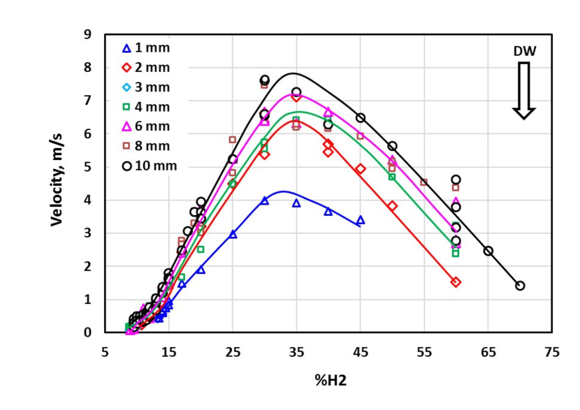
(a)

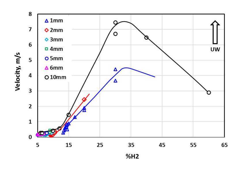
(b)

Figure 4: Drift velocity for downward (DW) and upward (UW) propagation. See also Kuznetsov et al. [9 Fig. 7]. The flame-ball regime corresponds to ultralean flames ($\%{H_{2}}<20$).

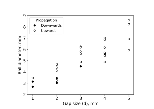
Figure 5: Flamelet diameter vs. gap size for one-headed flamelets.

Figure 6: Drift velocity $V$ vs. heat loss intensity $q$ for a planar flame.

3 Reduction to a free-boundary problem

The fingering patterns of Figs.1-3 are traces of self-drifting near circular reactive spots. They may be regarded as a 2D version of familiar self-drifting 3D flame-balls [10, 11] (see also comment ii) of Sec. 5). This observation in turn suggests the possible existence of individual self-drifting 2D flame-balls described by time-independent reaction-diffusion equations,

$$V\dfrac{\partial T}{\partial\eta}=\dfrac{\partial^{2}T}{\partial\xi^{2}}+\dfrac{\partial^{2}T}{\partial\eta^{2}}+(1-\sigma)\Omega-q(T-\sigma),$$ (4)

$$V\dfrac{\partial C}{\partial\eta}=\frac{1}{Le}\left(\dfrac{\partial^{2}C}{\partial\xi^{2}}+\dfrac{\partial^{2}C}{\partial\eta^{2}}\right)+(1-\sigma)\Omega,$$ (5)

subjected to boundary conditions,

$$T(\xi^{2}+\eta^{2}\to\infty)=\sigma,\;C(\xi^{2}+\eta^{2}\to\infty)=1.$$ (6)

Here $\xi=x$, $\eta=y+Vt$, and $V$ is an eigen-value of the problem. For theoretical analysis it is technically advantageous to employ the familiar large-activation-energy $(N\gg 1)$ near-equidiffusive $(Le^{-1}-1\ll 1)$ approach where the reaction-diffusion system (4) and (5) is reduced to a free-boundary problem [12]. There, the reaction rate $\Omega$ transforms into a localized source distributed along the interface $\eta=R(\theta)\cos{\theta}$, $\xi=R(\theta)\sin{\theta}$. Eqs. (4) (5) translate into the familiar set of equations for the reduced temperature $\Theta$ and excess-enthalpy $S$,

$$V\dfrac{\partial\Theta^{(0)}}{\partial\eta}=\dfrac{\partial^{2}\Theta^{(0)}}{\partial\xi^{2}}+\dfrac{\partial^{2}\Theta^{(0)}}{\partial\eta^{2}},$$ (7)

$$V\dfrac{\partial S}{\partial\eta}=\dfrac{\partial^{2}\left(S-\alpha\Theta^{(0)}\right)}{\partial\xi^{2}}+\dfrac{\partial^{2}\left(S-\alpha\Theta^{(0)}\right)}{\partial\eta^{2}}-\nu\Theta^{(0)}$$ (8)

Here $\Theta=(T-\sigma)/(1-\sigma)$; $S=(\Theta+C-1)\beta$; the Zeldovich number $\beta=(1-\sigma)N$, is assumed to be large; $\alpha=\left(Le^{-1}-1\right)\beta$, $\nu=q\beta$ are assumed to be finite; $\Theta^{(0)}=\Theta(\beta\to\infty)$.

At the reactive interface, $\xi^{2}+\eta^{2}=R^{2}(\theta)$, the following conditions are held,

$$\left[S\right]^{+}_{-}=0,\;\Theta^{(0)}=1,$$ (9)

$$\left[\dfrac{\partial S}{\partial n}\right]^{+}_{-}=\alpha\left[\dfrac{\partial\Theta^{(0)}}{\partial n}\right]^{+}_{-},$$ (10)

$$\left[\dfrac{\partial\Theta^{(0)}}{\partial n}\right]^{+}_{-}=-\left(1+\dfrac{1}{R^{2}}\left(\dfrac{\partial R}{\partial\theta}\right)^{2}\right)^{1/2}\exp{\left(\dfrac{S}{2}\right)}.$$ (11)

Here $\partial/\partial n$ is the normal derivative. And,

$$\Theta^{(0)}\to 0,\;S\to 0,$$ (12)

at $\xi^{2}+\eta^{2}\to\infty$. Within the flame-ball interface the deficient reactant is assumed to be fully consumed,

$$C\left(\xi^{2}+\eta^{2}\leq R^{2}(\theta)\right)=0.$$ (13)

Finally we observe that Eq. (7) allows for the exact solution which in polar coordinates ($\eta=r\cos{\theta},\xi=r\sin{\theta}$) reads, [13, 14],

$$\Theta^{(0)}(r,\theta)=\sum_{m}\exp{\left(kr\cos{\theta}\right)}\cos{\left(m\theta\right)}\cdot$$

$$\cdot\left[A_{m}K_{m}(kr)+B_{m}I_{m}(kr)\right]+H.$$ (14)

Here $K_{m}$, $I_{m}$ are modified Bessel functions of first and second kind, $k=V/2$, and $A_{m}$, $B_{m}$, $H$ are parameters to be determined by conditions at $r=0$, $r=\infty$ and $r=R(\theta)$.

4 Reduction to a 1D model

4.1 General

The 2D free-boundary problem (7) - (13) is still too difficult for a straightforward analytical treatment. We therefore propose to consider its low-mode allocation-like reduction to a 1D model that we believe will keep enough contact with the original 2D formulation. More specifically, in the 1D approach $\Theta,C,S$ are projected on the $\eta$ - axis running through the center of the flame ball (Fig. 7).

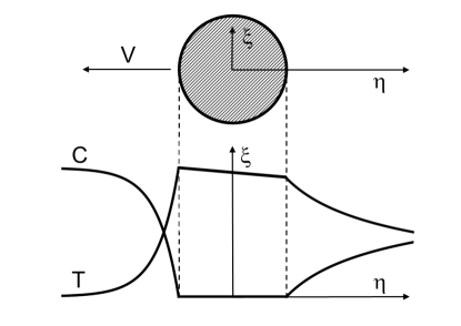
Figure 7: Up: Top sketch view of the flamelet in a plane parallel both to the paper and to the plates of the Hele-Shaw cell. Down: Profiles of temperature, $T$, and concentration, $C$, through the center of the flame-ball.

There the interior of the flame-ball covers the interval $-R<\eta<R$. In the expansion (14) we will keep only the leading order terms corresponding to $m=0$. Moreover, we will set $\theta=0$ for $\eta>0$ and $\theta=\pi$ for $\eta<0$. Conditions (9) - (13) on the flame-ball interface $\eta=\pm R$ and $\eta=\pm\infty$ thus become,

$$\left[S\right]^{+}_{-}=0,\;\Theta^{(0)}=1,$$ (15)

$$\left[\dfrac{\partial\Theta^{(0)}}{\partial\eta}\right]^{+}_{-}+\exp{\left(\dfrac{S}{2}\right)}=0,$$ (16)

$$\left[\dfrac{\partial S}{\partial\eta}\right]^{+}_{-}=\alpha\left[\dfrac{\partial\Theta^{(0)}}{\partial\eta}\right]^{+}_{-},$$ (17)

$$\Theta^{(0)}\left(\eta=\pm\infty\right)=0,\;S\left(\eta=\pm\infty\right)=0.$$ (18)

And

$$C\left(-R<\eta<R\right)=0.$$ (19)

For the leading order approximation, $\beta\gg 1$,

$$\Theta^{(0)}\left(\eta>R\right)=\exp{\left[k(\eta-R)\right]}\dfrac{K_{0}(k\eta)}{K_{0}(kR)},$$ (20)

$$\Theta^{(0)}\left(\eta<-R\right)=\exp{\left[k(\eta+R)\right]}\dfrac{K_{0}(-k\eta)}{K_{0}(kR)},$$ (21)

$$\Theta^{(0)}\left(-R<\eta<R\right)=1,$$ (22)

$$C^{(0)}\left(\eta\right)=1-\Theta^{(0)}\left(\eta\right).$$ (23)

For the higher order uniform approximation needed for evaluation of $S=(\Theta+C-1)\beta$,

$$\Theta\left(\eta>R\right)=\left[1+\beta^{-1}S(R)\right]\cdot$$

$$\cdot\exp{\left[k(\eta-R)\right]}\dfrac{K_{0}\left((k^{2}+q)^{\frac{1}{2}}\eta\right)}{K_{0}\left((k^{2}+q)^{\frac{1}{2}}R\right)},$$ (24)

$$\Theta\left(\eta<-R\right)=\left[1+\beta^{-1}S(-R)\right]\cdot$$

$$\cdot\exp{\left[k(\eta+R)\right]}\dfrac{K_{0}\left(-(k^{2}+q)^{\frac{1}{2}}\eta\right)}{K_{0}\left((k^{2}+q)^{\frac{1}{2}}R\right)},$$ (25)

$$\Theta\left(-R<\eta<R\right)=1+\beta^{-1}S\left(-R<\eta<R\right),$$ (26)

$$S\left(-R<\eta<R\right)=A+B\exp{(k\eta)}I_{0}(k|\eta|)$$

$$\mspace{145.0mu}-\nu\eta/2k,$$ (27)

where,

$$A=\left[S(R)+S(-R)\right]$$

$$-\dfrac{1}{2}BI_{0}(kR)\left[\exp{(kR)}+\exp{(-kR)}\right]$$ (28)

$$B=\dfrac{\nu R+S(R)-S(-R)}{kI_{0}(kR)\left[\exp{(kR)}-\exp{(-kR)}\right]},$$ (29)

$$C(\eta>R)=1-\exp{\left[kLe(\eta-R)\right]}\dfrac{K_{0}(kLe\eta)}{K_{0}(kLeR)},$$ (30)

$$C(\eta<\!-R)=1-\exp{\left[kLe(\eta+R)\right]}\dfrac{K_{0}(-kLe\eta)}{K_{0}(kLeR)},$$ (31)

$$C(-R<\eta<R)=0.$$ (32)

The uniform approximation employed in the above equations allows meeting the boundary conditions $\Theta(\eta\to\infty)=0$, $S(\eta\to\infty)=0$, behind the self-drifting flamelet, where $\eta\sim\beta$.

4.2 Results

Eqs. (20) - (32) meet the continuity conditions (15) at $\eta=\pm R$. Substituting Eqs. (20) - (32) into jump conditions (16), (17) one ends up with four algebraic relations for four unknown parameters $V=2k$, $R$, $S(R)$, $S(-R)$ as functions of $\alpha$, $\nu$, $\beta$ (Figs. 9, 9, 10). More technical details and the numerical procedure employed for the emerging algebraic problem are presented in the earlier version of the paper [15].

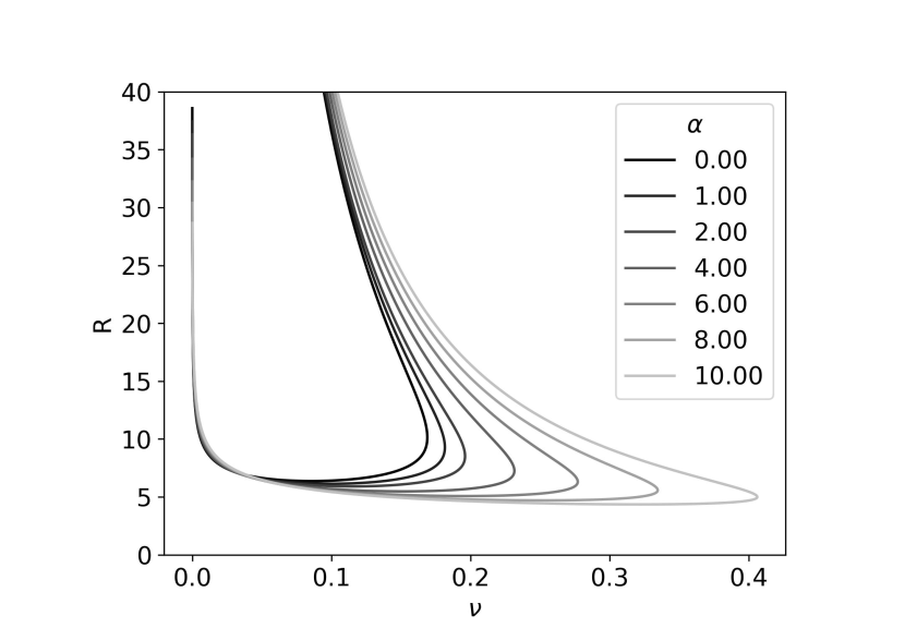
Figure 8: Locus of the flamelet radii, $R$, as a function of the heat losses, $\nu$, for different Lewis number parameters, $\alpha$.

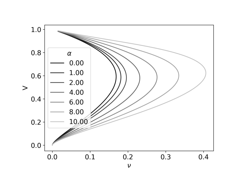
Figure 9: Locus of the velocities, $V$, as a function of the heat losses, $\nu$, for different Lewis number parameters, $\alpha$.

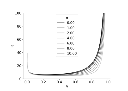
Figure 10: Locus of the flamelet radii, $R$, as a function of velocity, $V$, for different Lewis number parameters, $\alpha$.

One can draw several conclusions from the results obtained.

1. Parameter $\alpha$ strongly affects $V(\nu)$, $R(\nu)$ - dependencies. The heat loss intensity at the quenching (turning) point, $\nu_{q}$, increases with the decrease of the Lewis number, $Le\simeq 1-\alpha/\beta$.

2. At $\nu<\nu_{q}$ the multiplicity of $V(\nu)$, $R(\nu)$ is observed. A similar non-uniqueness is known to occur in planar ($R=\infty$) non-adiabatic flames which leads to the $\alpha$-independent relation between $V$ and $\nu$, $V^{2}\ln{\left(1/V\right)}=\nu$, [16].

3. Once the solutions for $V(\nu)$, $R(\nu)$ for a certain $\alpha$ are available, one can plot spatial profiles of all state variables involved. For brevity we depict here only $\Theta(\eta)$ for the upper and lower branches of $V(\eta)$ (Figs. 12, 12). A significant drop of temperature $\Theta$ at the rear side ($\eta=R$) of the self-drifting flame-ball might explain the horseshoe shape of the advancing flamelet. The latter is often perceived as a local extinction (opening ) of the front.

   

   Figure 11: Profiles of $\Theta$ for $\alpha=1$, $\beta=10$ and different values of $\nu$ for the upper branch of $V(\nu)$.

   

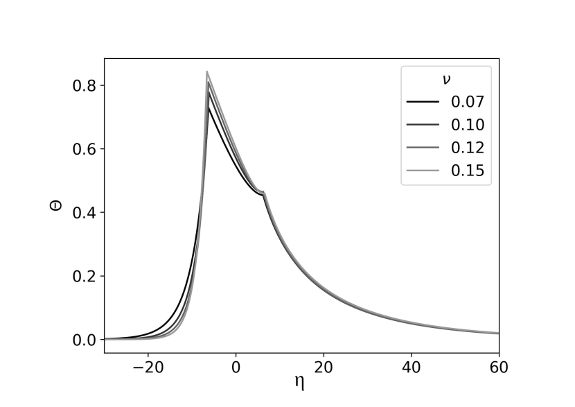
   Figure 12: Profiles of $\Theta$ for $\alpha=1$, $\beta=10$ and different values of $\nu$ for the lower branch of $V(\nu)$.

5 Concluding remarks

1. In constructing a workable approximate solution we truncated the series involving an infinite number of terms, as in Eq. (14), setting $m$ at zero, to deal with sums involving only a finite number of terms.

2. There is an important distinction between the 3D and effectively 2D situation typical of large aspect ratio Hele-Shaw cells. The 3D case allows for stationary spherical flame-balls which may bifurcate into a self-drifting mode [10, 11]. In the 2D case, the non-drifting circular flame-balls are ruled out. They cannot meet boundary conditions at infinity (due to the logarithmic tail of the associated concentration profiles [7]). So, in narrow gaps 2D self-drifting flame-balls should emerge not as a bifurcation but rather as the only way for the 2D flame-balls to exist.

3. In the present study the pattern of the flame disintegration is controlled by the heat loss intensity $q=(\pi\ell_{th}/d)^{2}$, which in turn may be controlled by the width of the Hele-Shaw gap ($d$) or the mixture composition (% $H_{2}$ or $\ell_{th}$) [4, 9, 17].

4. The reaction-diffusion model of Sec. 2 does not seem capable of reproducing two-headed flamelets. The latter is often observed experimentally [4, 18] as well as in simulations of more sophisticated models that consider the burned gas thermal expansion [7, 19] and are therefore susceptible to Darrieus-Landau instability. At the moment the issue of two-headed flamelets remains unexplained.

5. The present work is devoted to estimates of the propagation velocity of an individual flame-ball in a flat channel. It would be interesting to extend the analysis over the collective propagation of a group of flame-balls appearing in Figs. 1-3, and where the flamelets are competing for common fuel and mutual heating of one another. A mean-field type of approach as the developed by D’Angelo and Joulin [20] or Williams and Grcar [21] seems particularly promising.

6. In the present study flame-balls emerge in gaseous premixtures as an extreme case of diffusive-thermal instability where invariably $Le<1$. A similar pattern is observed in smoldering burning of thin solid sheets with and without imposed air flows [22-28]. There, similar to the gaseous systems, the effective Lewis number is considerably below unity [28]. It would be interesting to extend the 1D approach of this paper also to the smoldering problem.

Declaration of competing interest

The authors declare that they have no known competing financial interests or personal relationships that could have appeared to influence the work reported in this paper.

Acknowledgements

This research was supported in part by the US-Israel Binational Science Foundation (Grant 2020-005).

References

- [1] E.-A. Tingas, A. M. K. P. Taylor, Hydrogen for future thermal engines, Springer, 2023.
- [2] F. A. Williams, Combustion theory, Perseus Book Pub., Reading, Massachusetts, 1985.
- [3] P. Clavin, G. Searby, Combustion waves and fronts in flows: flames, shocks, detonations, ablation fronts and explosion of stars, Cambridge University Press, 2016.
- [4] F. Veiga-López, M. Kuznetsov, D. Martínez-Ruiz, E. Fernández-Tarrazo, J. Grune, M. Sánchez-Sanz, Unexpected propagation of ultra-lean hydrogen flames in narrow gaps, Phys. Rev. Lett. 124 (2020) 174501.
- [5] M. Kuznetsov, J. Grune, Experiments on combustion regimes for hydrogen/air mixtures in a thin layer geometry, International Journal of Hydrogen Energy 44 (17) (2019) 8727–8742.
- [6] L. Kagan, G. Sivashinsky, Self-fragmentation of nonadiabatic cellular flames, Combust. Flame 108 (1997) 220–226.
- [7] D. Martínez-Ruiz, F. Veiga-López, D. Fernández-Galisteo, V. N. Kurdyumov, M. Sánchez-Sanz, The role of conductive heat losses on the formation of isolated flame cells in Hele-Shaw chambers, Combust. Flame 209 (2019) 187–199.
- [8] A. Dejoan, D. Fernández-Galisteo, V. N. Kurdyumov, Numerical study of the propagation patterns of lean hydrogen-air flames under confinement, 29th ICDERS. July 23-28, SNU Siheung, Korea, 2023.
- [9] M. Kuznetsov, J. Yanez, F. Veiga-López, Near limit flame propagation in a thin layer geometry at low Peclet numbers, in: Proc. 18th Int. Conference on Flow Dynamics (ICFD 2021), no. OS18-8, 2022, pp. 688–692.
- [10] I. Brailovsky, G. Sivashinsky, On stationary and travelling flame balls, Combust. Flame 110 (1997) 524–529.
- [11] S. Minaev, L. Kagan, G. Joulin, G. Sivashinsky, On self-drifting flame balls, Combust. Theor. Model. 5 (2001) 609.
- [12] B. Matkowsky, G. Sivashinsky, An asymptotic derivation of two models in flame theory associated with the constant density approximation, SIAM J. App. Math. 37 (1979) 686–699.
- [13] H. Lamb, Hydrodynamics, Cambridge University Press, 1924.
- [14] S. Tomotika, T. Aoi, The steady flow of viscous fluid past a sphere and circular cylinder at small Reynolds numbers, Q. J. Mech. Appl. Math. 3 (1950) 141–161.
- [15] J. Yanez, L. Kagan, G. Sivashinsky, M. Kuznetsov, Modeling of 2D self-drifting flame-balls in Hele-Shaw cells, Combustion and Flame 258 (2023) 113059.
- [16] G. Sivashinsky, B. Matkowsky, On the stability of nonadiabatic flames, SIAM Journal on Applied Mathematics 40 (2) (1981) 255–260.
- [17] P. V.Moskalev, V. P. Denisenko, I. A. Kirillov, Classification and dynamics of ultralean hydrogen–air flames in horizontal cylindrical Hele–Shaw cells, Journal of Experimental and Theoretical Physics 137 (1) (2023) 104–113.
- [18] J. Y. Escanciano,M. Kuznetsov, F. Veiga-López, Characterization of unconventional hydrogen flame propagation in narrow gaps, Phys. Rev. E 103 (2021) 033101.
- [19] A. Domínguez-González, D. Martínez-Ruiz, M. Sánchez-Sanz, Stable circular and double-cell lean hydrogen-air premixed flames in quasi twodimensional channels, Proc. Combust. Inst. (2022).
- [20] Y. D’Angelo, G. Joulin, Collective effects and dynamics of non-adiabatic flame balls, Combustion Theory and Modelling 5 (1) (2001) 1.
- [21] F. A. Williams, J. F. Grcar, A hypothetical burning velocity formula for very lean hydrogen–air mixtures, Proc. Combust. Inst. 32 (1) (2009) 1351–1357.
- [22] Y. Zhang, P. Ronney, E. Roegner, J. Greenberg, Lewis number effects on flame spreading over thin solid fuels, Combust. Flame 90 (1992) 71–83.
- [23] O. Zik, Z. Olami, E. Moses, Fingering instability in combustion, Phys. Rev. Lett. 81 (1998) 3868.
- [24] T. Matsuoka, K. Nakashima, Y. Nakamura, S. Noda, Appearance of flamelets spreading over thermally thick fuel, Proc. Combust. Inst. 36 (2017) 3019–3026.
- [25] F. Zhu, Z. Lu, S. Wang, Y. Yin, Microgravity diffusion flame spread over a thick solid in step-changed low velocity opposed flows, Combust. Flame 205 (2019) 55–67.
- [26] J.Malchi, R. Yetter, S. Son, G. Risha, Nano-aluminum flame spread with fingering combustion instabilities, Proc. Combust. Inst. 31 (2) (2007) 2617–2624.
- [27] S. Olson, H. Baum, T. Kashiwagi, Finger-like smoldering over thin cellulosic sheets in microgravity, in: Symp. (Int.) Combust., Vol. 27, Elsevier, 1998, pp. 2525–2533.
- [28] Y. Uchida, K. Kuwana, G. Kushida, Experimental val idation of Lewis number and convection effects on the smoldering combustion of a thin solid in a narrow space, Combust. Flame 162 (5) (2015) 1957–1963.