DSEG-LIME - Improving Image Explanation by Hierarchical Data-Driven Segmentation

Abstract

Explainable Artificial Intelligence is critical in unraveling decision-making processes in complex machine learning models. LIME (Local Interpretable Model-agnostic Explanations) is a well-known XAI framework for image analysis. It utilizes image segmentation to create features to identify relevant areas for classification. Consequently, poor segmentation can compromise the consistency of the explanation and undermine the importance of the segments, affecting the overall interpretability. Addressing these challenges, we introduce DSEG-LIME (Data-Driven Segmentation LIME), featuring: i) a data-driven segmentation for human-recognized feature generation, and ii) a hierarchical segmentation procedure through composition. We benchmark DSEG-LIME on pre-trained models with images from the ImageNet dataset - scenarios without domain-specific knowledge. The analysis includes a quantitative evaluation using established XAI metrics, complemented by a qualitative assessment through a user study. Our findings demonstrate that DSEG outperforms in most of the XAI metrics and enhances the alignment of explanations with human-recognized concepts, significantly improving interpretability. The code is available under: https://github.com/patrick-knab/DSEG-LIME

Keywords Explainable AI (XAI)  $\cdot$ Foundation Models  $\cdot$ LIME

1 Introduction

Why should we trust you? Integration of AI-powered services into everyday scenarios, with or without the need for specific domain knowledge, is becoming increasingly common. An example is the image classification feature in smartphone photo galleries, which sorts images into various categories. For effective user engagement, accuracy and conformity to human understanding are crucial. Outsiders sometimes want to evaluate these systems’ performance post-deployment to quantify their functionality, specifically whether the AI accurately identifies different objects as separate concepts. The derived question - ’Why should we trust the model?’ - directly ties into the utility of Local Interpretable Model-agnostic Explanations (LIME) [1]. LIME seeks to demystify AI decision-making by identifying key features that influence the output of a model, underlying the importance of the Explainable AI (XAI) research domain, particularly when deploying opaque models in real-world scenarios [2, 3, 4].

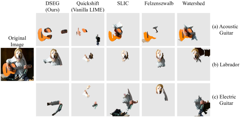
Figure 1: Segmentation Techniques within LIME. Illustrating the explanations generated by LIME [1] for EfficientNetB4 [5], employing a variety of segmentation methods. These include DSEG (ours) combined with SAM (Segment Anything) [6], Quickshift [7], SLIC (Simple Linear Iterative Clustering) [8], Felzenszwalb [9] and the Watershed algorithm [10]. The top predictions are ’Acoustic Guitar’ ($p$ = 0.31), ’Golden Retriever’ ($p$ = 0.24), and ’Electric Guitar’ ($p$ = 0.07).

Segmentation is key. LIME uses segmentation techniques to identify and generate features to determine the key areas of an image that are critical for classification. However, a challenge emerges when these segmentation methods highlight features that fail to align with identifiable, clear concepts or arbitrarily represent them. This issue is particularly prevalent with conventional segmentation techniques. These methods, often grounded in graph- or clustering-based approaches [11], were not initially designed for distinguishing between different objects within images, yet standard in LIME’s implementation [1]. Additionally, these methods struggle with creating a compositional object structure, where objects, like a guitar, are identified by their components, such as the body or headstock, limiting segmentation clarity and relevance.

Ambiguous explanations. The composition of the segmentation has a significant influence on the explanation’s quality [12]. Images with a multitude of segments often exhibit notable stability issues within LIME, where it is not uncommon to encounter two entirely contradictory explanations for the same instance - eroding trust in both LIME’s explanation and the reliability of the model being analyzed [13, 14, 15, 16, 4]. Moreover, humans often struggle to interpret the explanations, as the highlighted areas do not align with our intuitive understanding [17].

This work. In this paper, we address the challenges above by introducing DSEG-LIME (Data-driven Segmentation LIME), an adaptation of the LIME framework for image analysis across domains where specialized knowledge is not required. We substitute the conventional segmentation algorithm with a transformer-based foundation model, SAM [6]. We frequently refer to these foundation models as data-driven to denote their ability to generate features that more accurately capture concepts recognizable by humans derived from vast imagery data collections. Given the great segmentation ability of SAM, we implement a compositional object structure, adapting LIME’s feature generation with a novel hierarchical segmentation. This adaptation provides flexibility in the granularity of concepts, allowing users to specify the detail of LIME’s explanation, viewing a car as a whole or in parts like doors and windshields. This approach breaks down broad categorizations, enabling independent evaluation of each sub-concept.

Figure 1 demonstrates the motivation mentioned above by employing LIME, which generates explanations using various segmentation techniques, specifically focusing on an image of a dog playing the guitar. In this context, DSEG excels by more clearly highlighting features that align with human-recognizable concepts, distinguishing it from other methods.

Contribution. In summary, the two main contributions of our paper are outlined as follows: (i) We introduce DSEG-LIME, which enhances the LIME framework for image analysis by integrating foundation models, particularly SAM, to improve feature quality and achieve more accurate explanations. (ii) DSEG advances LIME by incorporating a compositional object structure, enabling hierarchical segmentation, which allows for adjustable feature granularity.

To validate our claims, we extensively evaluate DSEG versus other segmentation methods and enhancements within the LIME framework across multiple pre-trained image classification models. We incorporate a user study for qualitative analysis and differentiate between explaining (quantitative) and interpreting (qualitative) aspects. Recognizing that the explanations considered most intuitive by users may not always align with the operational logic of the AI models, diverging from human perception [18, 17], we enhance our evaluation with various quantitative performance metrics widely used in XAI research [19].

2 Foundations of LIME

In this section, we introduce the LIME framework [1], providing its theoretical foundation and functionality to establish the context for our approach.

Notation. We consider the scenario where we deal with imagery data. Let $\mathbf{x}\in\mathcal{X}$ represent an image within a set of images, and let $\mathbf{y}\in\mathcal{Y}$ denote its corresponding label in the output space with logits $\mathcal{Y}\subseteq\mathbb{R}$ indicating the labels in $\mathcal{Y}$. We denote the neural network designed for explanation by $f:\mathcal{X}\rightarrow\mathcal{Y}$. This network functions by accepting an input $\mathbf{x}$ and producing an output in $\mathcal{Y}$, which signifies the probability $p$ of the instance being classified into a specific class.

2.1 Local Interpretable Model-agnostic Explanations

LIME is a prominent XAI framework designed to explain the decisions of a neural network $f$ in a model-agnostic and instance-specific (local) manner. It applies to various modalities, including images, text, and tabular data [1]. In the following, we will briefly review LIME’s algorithm for treating images.

Feature Generation. The technique involves training a local, interpretable surrogate model $g\in G$, where $G$ is a class of interpretable models, such as linear models or decision trees, which approximates $f$’s behavior around an instance $\mathbf{x}$ [1]. This instance needs to be transformed into a set of features that can be used by $g$ to compute the importance score of its features. In the domain of imagery data, segmentation algorithms segment $\mathbf{x}$ into a set of superpixels $s_{0}...s_{d}\in\mathcal{S}^{D}$, done by conventional techniques [9, 7, 8, 10]. We treat these superpixels as the features for which we calculate their importance score. This step reflects the problematic process mentioned in Fig. 1, which forms the basis for the quality of the features that influence the explanatory quality of LIME.

Sample Generation. For sample generation, the algorithm manipulates superpixels by toggling them randomly. Specifically, each superpixel $s_{i}$ is assigned a binary state, indicating this feature’s visibility in a perturbed sample $\mathbf{z}$. The presence (1) or absence (0) of these features is represented in a binary vector $\mathbf{z^{\prime}_{i}}$, where the $i$-th element corresponds to the state of the $i$-th superpixel in $\mathbf{z}$. When a feature $s_{i}$ is absent (i.e., $s_{i}=0$), its pixel values in $\mathbf{z}$ are altered. This alteration typically involves replacing the original pixel values with a reference value, such as the mean pixel value of the image or a predefined value (e.g., black pixels) [1, 16]. Consequently, the modified instance $\mathbf{z}$, while retaining the overall structure of the original image $\mathbf{x}$, exhibits variations in its feature representation due to these alterations.

Feature Attribution. LIME employs a proximity measure, denoted as $\pi_{\mathbf{x}}$, to assess the closeness between the predicted outputs $f(\mathbf{z})$ and $f(\mathbf{x})$, which is fundamental in assigning weights to the samples. In the standard implementation of LIME, the kernel $\pi_{\mathbf{x}}(\mathbf{z})$ is defined as follows:

$$\pi_{\mathbf{x}}(\mathbf{z^{\prime}})=\exp\left(-\frac{D(\mathbf{x^{\prime}},\mathbf{z^{\prime}})^{2}}{\sigma^{2}}\right),$$ (1)

where $\mathbf{x^{\prime}}$ is a binary vector, all states are set to 1, representing the original image $\mathbf{x}$. $D$ represents the $L2$ distance, given by $D(\mathbf{x^{\prime}},\mathbf{z^{\prime}})=\sqrt{\sum_{i=1}^{n}(\mathbf{x^{\prime}}_{i}-\mathbf{z^{\prime}}_{i})^{2}}$ and $\sigma$ being the width of the kernel. Subsequently, LIME trains a linear model, minimizing the loss function $\mathcal{L}$, which is defined as:

$$\mathcal{L}(f,g,\pi_{\mathbf{x}})=\sum_{\mathbf{z},\mathbf{z^{\prime}}\in\mathcal{Z}}\pi_{\mathbf{x}}(\mathbf{z})\cdot(f(\mathbf{z})-g(\mathbf{z^{\prime}}))^{2}$$ (2)

In this equation, $\mathbf{z}$, and $\mathbf{z^{\prime}}$ are sampled instances from the perturbed dataset $\mathcal{Z}$, and $g$ is the interpretable model being learned [1, 16]. The interpretability of the model is derived primarily from the coefficients of $g$. These coefficients quantify the influence of each feature on the model’s prediction, with each coefficient’s magnitude and direction (positive or negative) indicating the feature’s relative importance and effect.

3 DSEG-LIME

In this section, we will integrate the two contributions of DSEG-LIME: first, the substitution of traditional feature generation with a data-driven segmentation approach (Section 3.1), and second, the establishment of a hierarchical structure that organizes segments in a compositional manner (Section 3.2).

Figure 2: Pipeline of DSEG in LIME. Illustrating the LIME pipeline for image analysis, detailing the integration of DSEG and its specific steps - dashed lines represent the choice between applying DSEG or not.

3.1 Data-Driven Segmentation Integration

DSEG-LIME improves the LIME feature generation phase by incorporating data-driven transformer-based segmentation models, outperforming conventional graph- or cluster-based segmentation techniques in creating recognizable image segments across various domains. Specifically, our approach utilizes SAM (Segment Anything) [6] due to its remarkable capability to segment images across diverse areas. The integration of DSEG within the LIME framework is depicted in Fig. 2, following the processes outlined in Section 2. Here, the application of SAM during the feature generation phase influences the generation of superpixels/features $\mathcal{S}^{D}$. Consequently, this change affects both the loss in Eq. 2 and the proximity of the perturbed instances in Eq. 1 that improves the approximation of an interpretable model $g$ to explain the instance $\mathbf{x}$ of model $f$.

3.2 Hierarchical Segmentation

SAM’s segmentation capability, influenced by its design and hyperparameters, allows for both fine and coarse segmentations of an image [6]. The technique has the ability to segment a human-recognized concept at various levels, from the entirety of a car to its components, such as doors or windshields. This multitude of segments enables the composition of a concept into its sub-concepts, as shown in Fig. 4(a) - creating a hierarchical segmentation. We enrich the LIME framework with this hierarchical segmentation, allowing users to specify the granularity of segments for more tailored explanations and enabling the surrogate model to learn about features driven by human-recognizable concepts. In the following, we explain the steps of DSEG, shown in Fig. 2, to explain an image with LIME using SAM and hierarchical segmentation. Figure 3 shows the outputs of the intermediate steps in DSEG.

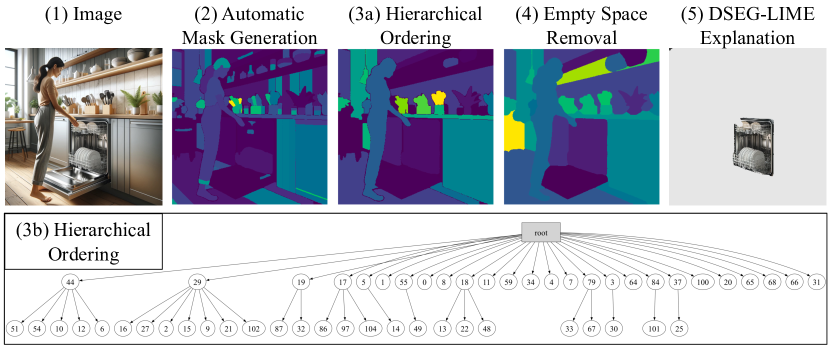
Figure 3: Visualized DSEG Pipeline. Image (1) serves as the initial input, leading to its automatic segmentation depicted in (2). The hierarchical tree generated from this segmentation is illustrated in (3b), and (3a) showcasing the mask composed of first-order nodes. Image (4) displays the finalized mask created after eliminating empty spaces, which is fed back into the sample generation of LIME. Image (5) represents the resultant explanation within the DSEG-LIME framework. A generative model generated the instance [20] in three distinct variations: featuring a woman, featuring a man, and without any person, aiming to detect potential gender biases in the EfficientNetB4 model.

Automatic Mask Generation. In the following, we denote the technique SAM by $\zeta$. SAM can be used by prompting with points, marking areas, or automatically segmenting all visible elements in an image [6]. For DSEG, we utilize the last prompt, automated mask generation, since we want to segment the whole image for feature generation. The process can be expressed as follows:

$$M_{\text{auto}}=\zeta(\mathbf{x},G_{\text{grid}})\text{, with }\mathcal{S^{D}}=M_{\text{auto}},$$ (3)

where $\mathbf{x}$ is the input image and $G_{\text{grid}}$ is a grid overlay parameterized by the number of points per side, which facilitates automated segmentation. The output $M_{\text{auto}}$ represents the mask generated, as illustrated Fig. 3 (2).

Small Cluster Removal. SAM generates segments of varying sizes. We define a threshold $\theta$ such that segments with pixel-size below $\theta$ are excluded:

$$\mathcal{S^{\prime}}=\{s_{i}\in\mathcal{S^{D}}\,|\,\text{size}(s_{i})\geq\theta\}.$$ (4)

In this study, we set $\theta=500$ to reduce the feature set. The remaining superpixels in $\mathcal{S^{\prime}}$ are considered for feature attribution. SAM also allows the removal of small segments. But in DSEG, we enable user-driven segment exclusion post-processing, granting control over the granularity within the hierarchy and ensuring that users can adjust segmentation to their needs, thus enhancing the method’s flexibility.

Hierarchical Ordering. Given the fact of having overlapping segments, we impose a tree hierarchical structure $\mathcal{T}=(\mathcal{V},\mathcal{E})$. The nodes $v\in\mathcal{V}$ denote segments in $\mathcal{S^{\prime}}$, and the edges $(u,v)\in\mathcal{E}$ encode the hierarchical relationship between segments. This hierarchical ordering process $H(\mathcal{S^{\prime}})$ is a composition of the relative overlap of the segments, defined as:

$$H(\mathcal{S^{\prime}})=\text{BuildHierarchy}(\mathcal{S^{\prime}},\text{OverlapMetric}),$$ (5)

where OverlapMetric quantifies the extent of overlap between two segments $s_{1},s_{2}\in\mathcal{S^{\prime}}$ defined by

$$\text{OverlapMetric}(s_{1},s_{2})=\frac{|s_{1}\cap s_{1}|}{|s_{2}|}.$$ (6)

The hierarchy prioritizes parent segments (e.g., person) over child segments (e.g., clothing), as depicted (3a) in Fig. 3. Each node represents one superpixel with its unique identifier. In DSEG-LIME, the depth of the hierarchy determines the explanation’s granularity. For the scope of this paper, we concentrate on the first-order hierarchy, representing primary nodes as shown in (3b) of Fig. 3. At a hierarchy depth of two, we focus on the top $k$ significant nodes identified during the initial feature attribution phase, as illustrated in Fig. 2. This method does not encompass all nodes at depth two but concentrates on the children of the top $k$ significant nodes. Figure 4(a) illustrates the explanations at depths one and two for the chosen class, providing insight into the granularity of the explanations.

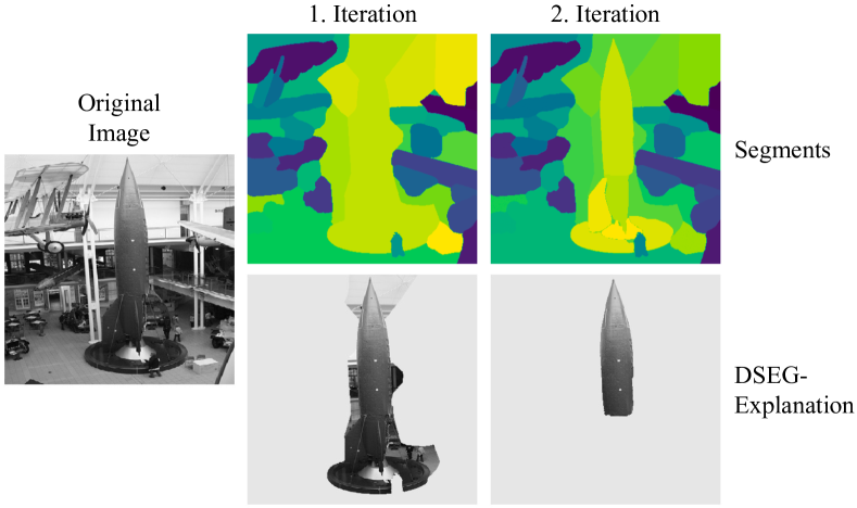
(a) 2nd Iteration of DSEG-LIME. Visualizing DSEG’s explanations of a projectile. It includes the first iteration’s explanation along with its corresponding segmentation map. Additionally, similar details are provided for the second iteration procedure, highlighting the upper part of a projectile as an explanation.

(b) Segmentation Stability. Illustrating a comparison between DSEG and other segmentation techniques applied in LIME, all utilizing an identical number of samples. DSEG exhibits greater stability compared to other segmentation techniques. Notably, the DSEG explanation distinctly highlights the segment representing a gorilla as the most definitive.

Figure 4: DSEG-LIME Explanations Showcasing explanations of DSEG-LIME and other segmentation techniques within LIME for stability and DSEG’s second iteration performance.

Empty Space Removal. In hierarchical segmentation, some regions occasionally remain unsegmented. We refer to these areas as $R_{\text{unseg}}$. To address this, we employ the nearest neighbor algorithm, which assigns each unsegmented region in $R_{\text{unseg}}$ to the closest segment within the set $\mathcal{S^{\prime}}$:

$$\mathcal{S^{\prime}}=\text{NearestNeighbor}(R_{\text{unseg}},\mathcal{S^{\prime}}).$$ (7)

Although this modifies the distinctiveness of concepts, it enhances DSEG-LIME’s explanatory power. The final mask, integrating these modifications, is then used in the context of LIME (Fig. 2), as shown in (4) of Fig. 3 and the corresponding explanation for the class ’dishwasher’ in (5).

4 Related Work

Instability of LIME. The XAI community widely recognizes the instability in LIME’s explanations [13]. This instability stems from LIME’s design, which aims to identify the most crucial features for a single prediction. Figure 4(b) shows the features instability of an exemplary image with different segmentation techniques within LIME. As the number of explainable features of instance $\mathbf{x}$ increases, the need for an extended set of perturbed data $\mathbf{x}^{\prime}$ to stabilize the local surrogate model also increases. Alvarez-Melis and Jaakkola [13] handled this issue by showing the instability of various XAI techniques when slightly modifying the instance $\mathbf{x}$ to be explained.

A direct improvement is Stabilized-LIME (SLIME) proposed by Zhou et al. [14] based on the central limit theorem to approximate the number of perturbations needed in the data sampling approach to guarantee improved explanation stability. Another LIME improvement regarding its stability is BayLIME by Zhau et al. [15], which exploits prior knowledge and Bayesian reasoning. GLIME [16] is a further LIME-based XAI technique that addressed this issue by employing an improved local and unbiased data sampling strategy, resulting in explanations with higher fidelity.

Segmentation Influence on Explanation. The segmentation algorithm utilized to sample data around the instance $\mathbf{x}$ strongly influences its explanation and directly affects the stability of LIME itself, as suggested by Chung et al. [21] and shown in Fig. 4(b). This is in line with the investigation by Schallner et al. [12] that examined the influence of different segmentation techniques in the medical domain, showing that the quality of the explanation depends on the underlying feature generation process. The work in [22] explored how occlusion and sampling strategies affect model explanations when integrated with segmentation techniques for XAI, including LRP (Layer-Wise Relevance Propagation) [23] and SHAP [24]. Their study highlights how different strategies provide unique explanations while evaluating the SAM technique in image segmentation. Sun et al. [25] used SAM within the SHAP framework to provide conceptually driven explanations.

Segmentation Hierarchy. The work of Li et al. [26] aimed to simulate the way humans structure segments hierarchically and introduced a framework called Hierarchical Semantic Segmentation Networks (HSSN), which approaches segmentation through a pixel-wise multi-label classification task. HIPPIE (HIerarchical oPen-vocabulary, and unIvErsal segmentation), proposed by Wang et al. [27], extended hierarchical segmentation by merging text and image data multimodally. It processes inputs through decoders to extract and then fuse visual and text features into enhanced representations.

5 Evaluation

In the following section, we will outline our experimental setup (Section 5.1) and introduce the XAI evaluation framework designed to assess DSEG-LIME both quantitatively (Section 5.2.1) and qualitatively (Section 5.3), compared to other LIME methodologies utilizing various segmentation algorithms. Subsequently, we discuss the limitations of DSEG (Section 5.4).

5.1 Experimental Setup

Segmentation Algorithms. Our experiment encompasses, along with SAM, four conventional segmentation techniques: Simple Linear Iterative Clustering (SLIC) [8], Quickshift (QS) [7], Felzenszwalb (FS) [9] and Watershed (WS) [10]. We carefully calibrate the hyperparameters of these techniques to produce segment counts similar to those generated by SAM. This calibration ensures that no technique is unfairly advantaged due to a specific segment count – for instance, scenarios where fewer but larger segments might yield better explanations than many smaller ones.

Models to Explain. The models investigated in this paper rely on pre-trained models, as our primary emphasis is on explainability. We chose EfficientNetB4 and EfficientNetB3 [5] as the ones treated in this paper, where we explain EfficientNetB4 and use EfficientNetB3 for a contrastivity check [19] (Section 5.2.1). To verify that our approach works on arbitrary pre-trained models, we also evaluated it using ResNet101 [28, 29] and VisionTransformer (ViT) [30]. Detailed results of these tests are given in the appendix.

Dataset. We use data from the ImageNet dataset [31], on which the models were trained [5, 28, 30]. We carefully selected images from various classes to ensure they represent the primary class while incorporating background elements, adding distinctiveness to the explanations. Additionally, to further challenge the segmentation algorithms, we created artificial images using the text-to-image model DALL-E [20]. Our final dataset consists of 20 instances, specifically chosen for a comprehensive evaluation of the techniques, both quantitatively and qualitatively. However, we want to emphasize that the selection of images is not biased towards any model.

Hyperparameters and Hardware Setup. The experiments were conducted on an Nvidia RTX A6000 GPU with 48 GB of VRAM, supported by a CPU with 1024 GB of RAM. We compare standard LIME, SLIME [14], GLIME [16], and BayLIME [15], all integrated with DSEG, using 256 samples per instance and a batch size of ten. For each explanation, up to three features are selected based on their significance, identified by values that exceed the average by more than 1.5 times the standard deviation. In BayLIME, we use the ’non-info-prior’ setting. For SAM, we configure it to use 32 points per side, and the conventional segmentation techniques are adjusted to achieve a similar segment count, as previously mentioned. In SLIC, we modify the number of segments and compactness; in Quickshift, the kernel size and maximum distance; in Felzenszwalb, the scale of the minimum size parameter; and in Watershed, the number of markers and compactness. Other hyperparameters remain at default settings to ensure a balanced evaluation across methods.

5.2 Quantitative Evaluation

We adapt the framework by Nauta et al. [19] to quantitatively assess XAI outcomes in this study, covering three domains: content, presentation, and user experience. In the content domain, we evaluate correctness, output completeness, consistency, and contrastivity. Presentation domain metrics like compactness and confidence are assessed under content for simplicity. The user domain, detailed in Section 5.3, includes a user study that compares our approach with other segmentation techniques in LIME.

5.2.1 Quantitative Metrics Definition.

In the following, we will briefly describe each metric individually to interpret the results correctly.

Correctness involves two randomization checks. The model randomization parameter check (Random Model) [32] tests if changing the random model parameters leads to different explanations. The explanation randomization check (Random Expl.) [33] examines if random output variations in the predictive model yield various explanations. For both metrics, in Table 1 we count the instances where explanations result in different predictions when reintroduced into the model under analysis.

The domain also utilizes two deletion techniques: single deletion [34] and incremental deletion [7, 35]. Single deletion serves as an alternative metric to assess the completeness of the explanation, replacing less relevant superpixels with a specific background to evaluate their impact on the model predictions [36]. After these adjustments, we note instances where the model maintains the correct image classification. Incremental deletion (Incr. Deletion) entails progressively eliminating features from most to least significant based on their explanatory importance. We observe the model’s output variations, quantifying the impact by measuring the area under the curve (AUC) of the model’s confidence, as parts of the explanation are excluded. This continues until a classification change is observed, and the mean AUC score for this metric is documented in Table 2.

Output Completeness measures whether an explanation covers the crucial area for accurate classification. It includes a preservation check (Preservation) [35] to assess whether the explanation alone upholds the original decision, and a deletion check (Deletion) [37] to evaluate the effect of excluding the explanation on the prediction outcome [36]. This approach assesses both the completeness of the explanation and its impact on the classification. The results are checked to ensure that the consistency of the classification is maintained. Compactness is also considered, highlighting that the explanation should be concise and cover all the areas necessary for prediction [38], reported by the mean value.

Consistency assesses explanation robustness to minor input alterations, like Gaussian noise addition, by comparing pre-and post-perturbation explanations for stability against slight changes (Noise Stability) [39, 40], using both preservation and deletion checks. For consistency of the feature importance score, we generate explanations for the same instance eight times (Rep. Stability), calculate the standard deviation $\sigma_{i}$ for each coefficient $i$, and then average all $\sigma_{i}$ values. This yields $\bar{\sigma}$, the average standard deviation of coefficients, and is reported as the mean score.

Contrastivity integrates several previously discussed metrics, aiming for target-discriminative explanations. This means that an explanation $e_{\textbf{x}}$ for an instance x from a primary model $f_{1}$ (EfficientNetB4) should allow a secondary model $f_{2}$ (EfficientNetB3) to mimic the output of $f_{1}$ as $f_{1}(\textbf{x})\approx f_{2}(e_{\textbf{x}})$ [41]. This approach checks the explanation’s utility and transferability across models, using EfficientNetB3 for preservation and deletion tests to assess consistency.

Table 1: Quantitative Summary - Classes. The table presents four quantitative areas and their metrics, comparing five segmentation techniques applied to EfficientNetB4: DSEG with SAM and comparative methods SLIC, Quickshift (QS), Felzenszwalb’s (FS), and Watershed (WS). Each is tested with four LIME framework variations: LIME (L), SLIME (S), GLIME (G), and BayLIME (B). The experimental setup and metrics are detailed in Section 5.1 and Section 5.2.1. The table includes class-based metrics, with a maximum score of 20 for each; higher scores indicate better performance, and the highest scores for each metric are highlighted in bold.

Domain	Metric	DSEG				SLIC				QS				FS				WS
		L	S	G	B	L	S	G	B	L	S	G	B	L	S	G	B	L	S	G	B
Correctness	Random Model	14	14	14	14	14	14	14	14	15	15	15	15	14	14	14	14	13	13	13	13
	Random Expl.	13	17	18	19	15	19	16	15	17	16	15	16	19	18	18	15	14	16	16	14
	Single Deletion	14	14	14	14	8	8	8	8	6	7	5	6	8	8	9	8	6	7	7	5
Output Completeness	Preservation	17	17	17	18	16	16	16	16	12	12	13	13	14	14	14	14	15	15	15	15
	Deletion	14	13	13	13	7	8	8	8	5	5	5	5	9	9	9	9	10	10	10	10
Consistency	Noise Stability	17	17	16	17	14	14	14	14	9	10	9	10	15	14	15	15	14	14	14	13
Contrastivity	Preservation	12	11	11	11	9	9	9	9	6	6	6	6	10	10	10	10	11	11	11	11
	Deletion	14	13	13	13	9	10	10	10	10	10	10	10	10	10	10	10	9	9	9	9

5.2.2 Quantitative Evaluation Results.

Table 1 presents the outcomes of all metrics associated with class-discriminative outputs. The numbers in bold signify the top results, with an optimal score of 20. We compare LIME (L) [1] with the LIME techniques discussed in Section 4, SLIME (S) [14], GLIME (G) [16], and BayLIME (B) [15] in combination with DSEG and the segmentation techniques from Section 5.1. The randomization checks of the correctness category confirm that the segmentation algorithm bias does not inherently affect any model. This is evidenced by the observation that most methods correctly misclassify when noise is introduced or when the model’s weights or predictions are shuffled. In contrast, DSEG consistently excels in other metrics detailed in the table, surpassing alternative segmentation methods irrespective of the LIME technique applied. In the output completeness domain, DSEG’s explanations more effectively capture the critical areas necessary for the model to accurately classify an instance, whether by isolating or excluding the explanation. This efficacy is supported by the single deletion metric, akin to the preservation check but with a perturbed background. Moreover, noise does not compromise the consistency of DSEG’s explanations. The contrastivity metric demonstrates DSEG’s effectiveness in creating explanations that allow another AI model to produce similar outputs in over half of the cases and outperform alternative segmentation approaches. Overall, the influence of the LIME feature attribution calculation does not vary much, but this is because we do not exceed 44 segments in the covered dataset for evaluation due to object-driven segmentation with a hierarchy depth of one.

Table 2: Quantitative Summary - Numbers. The table summarizes metrics from Section 5.2.1, focusing on those quantified by rational numbers like incremental deletion, compactness, representational stability, and average computation time across 20 examples, detailed in Section 5.1. In contrast to Table 1, lower values indicate better performance and the lowest values are printed in bold.

Metric	DSEG				SLIC				QS				FS				WS
	L	S	G	B	L	S	G	B	L	S	G	B	L	S	G	B	L	S	G	B
Incr. Deletion	0.33	0.18	0.19	0.34	0.38	0.31	0.30	0.35	0.43	0.44	0.44	0.41	0.40	0.42	0.45	0.43	0.32	0.36	0.36	0.32
Compactness	0.12	0.13	0.13	0.13	0.13	0.13	0.13	0.13	0.12	0.13	0.13	0.14	0.14	0.14	0.14	0.14	0.10	0.11	0.10	0.11
Rep. Stability	.008	.009	.009	.009	.008	.008	.009	.009	.011	.011	.012	.011	.011	.010	.011	.010	.012	.012	.012	.012
Time	45.62	50.25	45.82	50.84	17.80	18.05	19.46	17.58	28.85	26.09	25.88	25.47	17.37	18.61	18.82	18.59	16.93	17.85	19.77	17.34

Table 2 further demonstrates the proficiency of DSEG in capturing crucial areas for model output, particularly with incremental deletion where SLIME and GLIME lead. The numbers in bold stand for the lowest value, which indicates the best performance. Although compactness metrics show nearly uniform segment sizes across the techniques, Watershed’s smaller segments do not translate to better performance in other areas. Repeated experimentation suggests that stability is less influenced by the LIME variant and more by the segmentation approach, with SLIC and DSEG outperforming others. Further experiments show that DSEG outperforms SLIC regarding stability as the number of features increases. This advantage arises from the tendency of data-driven approaches to represent known objects uniformly as a single superpixel. Thus, if a superpixel accurately reflects the instance that the model in question predicts, it can be accurately and effortlessly matched with one or a few superpixels - such accurate matching leads to a more precise and more reliable explanation. Conventional segmentation algorithms often divide the same area into multiple superpixels, creating unclear boundaries and confusing differentiation between objects. Regarding computation time, the segmentation phase is the main differentiator; DSEG has longer processing times than the others. Nevertheless, it is important to note that computation time is also subject to the server load where the experiments were conducted, thereby introducing the possibility of slight variations.

5.3 Qualitative Evaluation - User Study

We conducted a survey to assess DSEG-LIME qualitatively. We based on the methodology proposed by Chromik and Schuessler [42] to design a robust user study for human subject evaluation in XAI, which was approved by the institute’s ethics council. It engaged 28 participants with various backgrounds, encompassing a wide range of ages, professional experiences, and varying degrees of familiarity with AI and XAI concepts. The study involved 20 images, each accompanied by five explanations and their model predictions of EfficientNetB4, all within the vanilla LIME framework as described in Section 5.1. Participants ranked the explanations from 1 (least effective) to 5 (most effective) based on how well they aligned with their intuitive understanding of the depicted object, with explanations presented randomly to prevent bias.

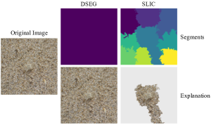
Figure 5: DSEG Fails. Demonstrating a scenario where DSEG fails to generate meaningful features for explanations (the whole image is one segment, in contrast to SLIC. The image shows a crab, which the model classifies as a ’hermit crab’ ($p$ = 0.17), highlighting the effectiveness of SLIC in this context compared to the limitations of DSEG.

5.3.1 Qualitative Evaluation Results.

The user study results are presented in Fig. 6. We show the cumulative maximum ratings in Fig. 6(a) and in Fig. 6(b) the median (in black), the interquartile range (1.5) and the mean (in red) for each segmentation technique. DSEG stands out in the absolute ratings, significantly exceeding the others. Similarly, in Fig. 6(b), DSEG achieves the highest rating, indicating its superior performance relative to other explanations. Therefore, while DSEG is most frequently rated as the best, it consistently ranks high even when it is not the leading explanation.

Balanced Evaluation. By using both quantitative and qualitative assessments, we ensure that the explanations are not only technically accurate and the models lead to correct classifications but are also consistent with human understanding while maintaining a balance to avoid over-emphasizing either technical precision or intuitive clarity [17].

(a) Best Rated Explanation. Accumulated number of best-selected explanations within the user study. DSEG was selected as the favorite, followed by Felzenszwalb and Watershed.

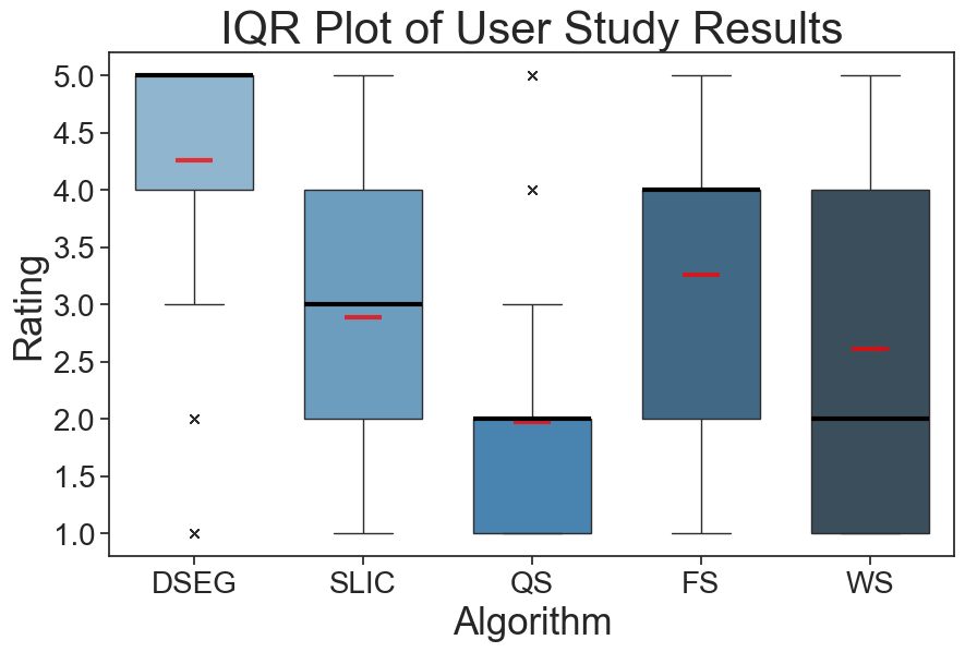
(b) IQR of Explanation’s Ratings. The IQR plot of the user study ratings is detailed, with the black line indicating the median and the red line representing the mean. This plot shows that DSEG received the highest ratings, while Watershed exhibited the broadest ratings distribution.

Figure 6: User Study Results. The user study ratings are visualized in two distinct figures, each employing a different form of data representation. In both visualizations, DSEG consistently outperforms the other techniques.

5.4 Limitations and Future Work

DSEG-LIME performs the feature generation directly on images before they are input into the model for explanation. For models like ResNet, designed for inputs of 224x224 pixels [28], the quantitative advantages of DSEG are less evident, as detailed in the appendix. The effectiveness of DSEG increases with larger image sizes. Furthermore, substituting superpixels with a specific value in preservation and deletion evaluations can introduce an inductive bias [4]. To reduce this bias, using a generative model to synthesize replacement areas could offer a more neutral alteration. Within DSEG, we use SAM for feature generation. Future exploration could involve testing alternative foundational models, such as DETR [43], alongside hierarchical segmentation techniques, as suggested in Section 4.

No Free Lunch. Although DSEG provides promising results in many domains, it is not always universally applicable. When domain-specific knowledge is crucial to identify meaningful features in LIME explanations or when the concept identification task is inherently complex, DSEG might not perform as effectively as traditional LIME segmentation methods. Figure 5 illustrates where DSEG does not provide meaningful explanations, while SLIC performs better.

6 Conclusion

In this study, we introduced DSEG-LIME, an extension to the LIME framework, incorporating a data-driven foundation model (SAM) for feature generation. This approach ensures that the generated features more accurately reflect human-recognizable concepts, enhancing the interpretability of explanations. Furthermore, we refined the process of feature attribution within LIME through an iterative method, establishing a segmentation hierarchy that contains the relationships between components and their subcomponents. Through a comprehensive two-part evaluation, split into quantitative and qualitative analysis, DSEG emerged as the superior method, outperforming other LIME-based approaches in most evaluated metrics.

The adoption of foundational models marks a significant step towards enhancing the interpretability of deep learning models. This advancement promises precise insights and paves the way for more transparent, understandable, and reliable artificial intelligence.

Appendix A Supplementary Model Evaluations

A.1 ResNet

Evaluation. In Table 3, we detail the quantitative results for the ResNet-224 model, comparing our evaluation with the criteria used for EfficientNetB4 under consistent hyperparameter settings. The review extends to a comparative analysis with EfficientNetB3, focusing on performance under contrastive conditions. The results confirm the EfficientNet results and show that the LIME techniques behave unpredictably in the presence of model noise or prediction shuffle despite different segmentation strategies. This indicates an inherent randomness in the model explanations. The single deletion metric showed that all XAI approaches performed below EfficientNetB4, with DSEG performing slightly better than its counterparts. However, DSEG performed best on other metrics, especially when combined with the SLIME framework, where it showed superior resilience to noise, distinguishing it from alternative methods.

Table 3: Quantitative Summary - Classes RES-224. The table presents the metrics consistently with those discussed for EfficientNet.

Domain	Metric	DSEG				SLIC				QS				FS				WS
		L	S	G	B	L	S	G	B	L	S	G	B	L	S	G	B	L	S	G	B
Correctness	Random Model	18	18	17	16	15	17	18	19	19	20	20	18	18	19	20	17	19	20	20	20
	Random Expl.	18	19	20	19	20	20	18	18	20	18	19	19	20	19	18	20	18	20	19	20
	Single Deletion	4	3	3	5	4	3	4	4	2	1	3	3	4	3	4	4	3	3	3	3
Output Completeness	Preservation	7	9	6	7	8	8	9	8	5	5	5	5	7	5	4	6	8	7	8	6
	Deletion	10	12	9	13	9	9	9	8	6	8	6	7	7	6	6	7	8	8	9	8
Consistency	Noise Stability	8	10	6	6	5	5	5	4	5	5	5	5	3	2	2	2	6	7	8	6
Contrastivity	Preservation	6	12	8	9	5	5	5	5	6	7	8	8	8	6	6	6	6	7	8	8
	Deletion	6	10	7	10	9	8	8	8	5	7	8	7	6	5	5	4	7	6	5	4

Table 4 presents further findings of ResNet. SLIME with DSEG yields the lowest AUC for incremental deletion, whereas Quickshift and Felzenszwalb show the highest. WS produces the smallest superpixels for compactness, contrasting with DSEG’s larger ones. The stability analysis shows that all segmentations are almost at the same level, with SLIC being the best and GLIME the best-performing over all. Echoing EfficientNet’s review, segmentation defines runtime, with DSEG being the most time-consuming. The runtime disparities between the ResNet and EfficientNet models are negligible.

Table 4: Quantitative Summary - Numbers RES-224. The table presents the metrics consistently with those discussed for EfficientNet.

Metric	DSEG				SLIC				QS				FS				WS
	L	S	G	B	L	S	G	B	L	S	G	B	L	S	G	B	L	S	G	B
Incr. Deletion	0.26	0.09	0.11	0.29	0.25	0.26	0.25	0.23	0.44	0.32	0.34	0.40	0.37	0.32	0.37	0.44	0.23	0.26	0.27	0.25
Compactness	0.24	0.20	0.21	0.18	0.15	0.15	0.14	0.15	0.16	0.16	0.16	0.16	0.16	0.18	0.15	0.15	0.13	0.14	0.13	0.13
Rep. Stability	.024	.023	.020	.022	.020	.020	.016	.021	.022	.021	.018	.021	.022	.022	.017	.022	.022	.021	.018	.020
Time	45.74	49.44	48.35	52.25	20.03	17.48	19.71	18.70	26.04	24.85	24.86	25.96	19.38	17.54	19.40	18.70	19.00	17.04	17.39	17.52

A.2 VisionTransformer

Evaluation. Table 5 provides the quantitative results for the VisionTransformer (ViT) model, employing settings identical to those used for EfficientNet and ResNet, with ViT processing input sizes of (384x384). The class-specific results within this table align closely with the performances recorded for the other models, further underscoring the effectiveness of DSEG. This consistency in DSEG performance is also evident in the data presented in Table 6. However, the ’Noise Stability’ metric shows poorer performance for both models than for EfficientNetB4, indicating that ViT and ResNet have greater difficulty when noise enters the input.

All experiments for ResNet and ViT were performed with the same hyperparameters defined for EfficientNetB4. We would like to explicitly point out that the performance of the quantitative results could be improved by defining more appropriate hyperparameters for both DSEG and conventional segmentation methods, as no hyperparameter search was performed for a fair comparison.

Table 5: Quantitative Summary - Classes VIT-384. The table presents the metrics consistently with those discussed for EfficientNet.

Domain	Metric	DSEG				SLIC				QS				FS				WS
		L	S	G	B	L	S	G	B	L	S	G	B	L	S	G	B	L	S	G	B
Correctness	Random Model	17	17	17	17	19	19	19	19	18	18	19	18	19	19	19	19	18	19	18	19
	Random Expl.	17	19	19	17	20	17	19	19	19	18	20	18	20	18	19	19	17	17	18	18
	Single Deletion	8	9	9	9	6	6	6	6	4	4	4	4	4	5	4	4	4	4	3	3
Output Completeness	Preservation	7	7	7	7	6	6	7	7	5	5	4	5	6	6	7	7	6	6	5	6
	Deletion	14	16	16	16	15	15	15	15	12	12	12	12	14	15	16	15	15	14	14	14
Consistency	Noise Stability	7	6	5	6	7	5	6	5	3	4	4	4	4	4	5	3	5	4	4	4
Contrastivity	Preservation	10	8	10	9	8	8	9	9	10	9	10	11	8	7	7	8	10	11	10	10
	Deletion	11	13	12	13	9	9	9	9	8	7	8	8	8	9	9	8	9	11	11	11

Table 6: Quantitative Summary - Numbers VIT-384. The table presents the metrics consistently with those discussed for EfficientNet.

Metric	DSEG				SLIC				QS				FS				WS
	L	S	G	B	L	S	G	B	L	S	G	B	L	S	G	B	L	S	G	B
Incr. Deletion	0.18	0.14	0.14	0.45	0.21	0.25	0.30	0.25	0.52	0.54	0.54	0.46	0.36	0.37	0.32	0.39	0.36	0.36	0.37	0.35
Compactness	0.17	0.17	0.17	0.16	0.12	0.12	0.12	0.12	0.14	0.14	0.13	0.13	0.13	0.12	0.13	0.12	0.11	0.11	0.10	0.11
Rep. Stability	.013	.013	.014	.013	.014	.014	.014	.014	.18	.018	.018	.017	.014	.014	.015	.014	.016	.016	.017	.016
Time	39.46	43.08	40.33	43.64	13.47	10.88	11.55	11.74	18.61	17.25	17.07	18.32	20.44	15.56	16.27	18.59	17.77	15.05	15.29	16.77

A.3 EfficientNetB4 with Depth of Two

Exemplary Explanations. DSEG-LIME introduces a hierarchical feature generation approach, allowing users to specify segmentation granularity via tree depth. Figure 7 displays five examples from our evaluation, with the top images showing DSEG’s explanations at a hierarchy depth of one and the bottom row at a depth of two. These explanations demonstrate that deeper hierarchies focus on smaller regions. However, the banana example illustrates a scenario where no further segmentation occurs if the concept, like a banana, lacks sub-components for feature generation, resulting in identical explanations at both depths.

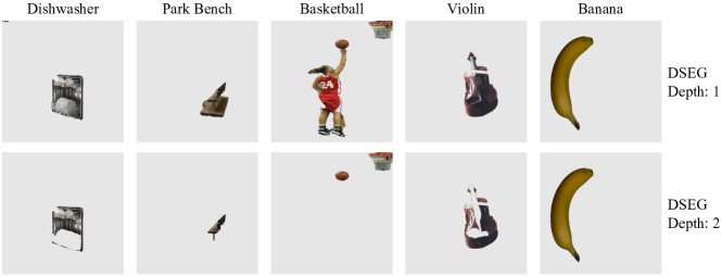
Figure 7: DSEG Depth 2 The figure displays exemplary images from the evaluation dataset, illustrating DSEG explanations at depth 2 of hierarchical segmentation. These images serve as complementary examples to the paper’s discussion on the projectile, enhancing the illustration of the concept.

Evaluation. In Table 7 and Table 8, we present the quantitative comparison between DSEG-LIME (depth two) using EfficientNetB4 and SLIC, as reported in the main paper. The hyperparameter settings were consistent across the evaluations, except for compactness. We established a minimum threshold of 0.05 for values to mitigate the impact of poor segmentation performance, which often resulted in too small segments. Additional segments were utilized to meet this criterion for scenarios with suboptimal segmentation. However, this compactness constraint was not applied to DSEG with depth two, since its hierarchical approach naturally yields smaller and more detailed explanations, evident in Table 8. The hierarchical segmentation of depth two slightly impacts stability, yet the method continues to generate meaningful explanations, as indicated by other metrics. Although our method demonstrated robust performance, it required additional time because the feature attribution process was conducted twice.

Table 7: Quantitative Summary - Classes Depth Two. The table showcases metrics for EfficientNetB4, specifically at a finer concept granularity; the hierarchical segmentation tree has a depth of two. Results reported pertain solely to integrating DSEG and SLIC within the scope of the LIME frameworks examined.

Domain	Metric	DSEG				SLIC
		L	S	G	B	L	S	G	B
Correctness	Random Model	16	16	16	16	14	14	14	14
	Random Expl.	16	18	18	14	15	19	16	15
	Single Deletion	9	10	9	11	8	8	8	8
Output Completeness	Preservation	16	13	14	13	16	16	16	16
	Deletion	6	10	10	9	7	8	8	8
Consistency	Noise Stability	13	14	14	15	14	14	14	14
Contrastivity	Preservation	14	12	12	13	9	9	9	9
	Deletion	6	6	7	6	9	10	10	10

Table 8: Quantitative Summary - Numbers Depth Two. The table showcases the numeric values in the same manner as in Table 7 but for numeric values.

Metric	DSEG				SLIC
	L	S	G	B	L	S	G	B
Incr. Deletion	0.40	0.26	0.15	0.16	0.38	0.31	0.30	0.35
Compactness	0.08	0.12	0.09	0.09	0.13	0.13	0.13	0.13
Rep. Stability	.011	.010	.011	.011	.008	.008	.009	.009
Time	75.22	72.72	73.61	75.02	17.80	18.05	19.46	17.58

Appendix B User Study

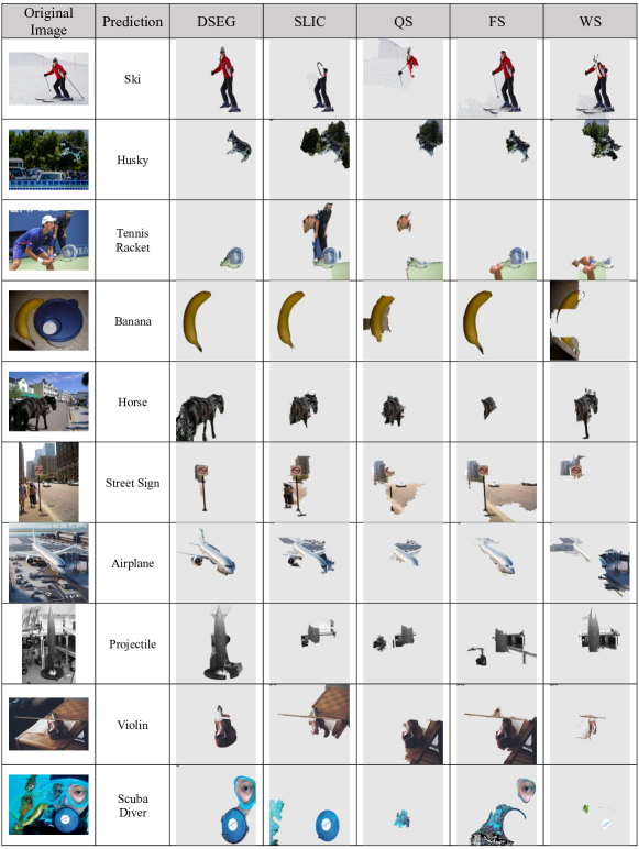
Figure 8: Images 1 - 10 The first ten examples of the user study conducted in this paper.

Instruction. Participants were tasked with the following question for each instance: "Please arrange the provided images that best explain the concept model’s prediction, ranking them from 1 (least effective) to 5 (most effective)." Each instance was accompanied by DSEG, SLIC, Watershed, Quickshift, Felzenszwalb, and Watershed within the vanilla LIME framework and the hyperparameters discussed in the experimental setup. These are also the resulting explanations used in the quantitative evaluation of EfficientNetB4. The explanations and instances provided to the participants are shown in Fig. 8 and Fig. 9.

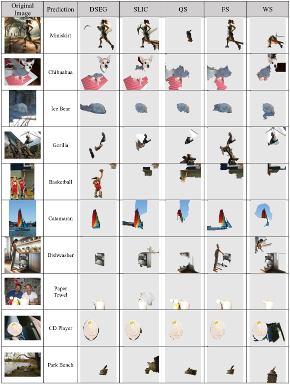
Figure 9: Images 11 - 20 The next ten examples of the user study conducted in this paper.

References

- [1] Marco Tulio Ribeiro, Sameer Singh, and Carlos Guestrin. "why should i trust you?": Explaining the predictions of any classifier. In Proceedings of the 22nd ACM SIGKDD International Conference on Knowledge Discovery and Data Mining, KDD ’16, page 1135–1144, New York, NY, USA, 2016. Association for Computing Machinery.
- [2] Alejandro Barredo Arrieta, Natalia Díaz-Rodríguez, Javier Del Ser, Adrien Bennetot, Siham Tabik, Alberto Barbado, Salvador Garcia, Sergio Gil-Lopez, Daniel Molina, Richard Benjamins, Raja Chatila, and Francisco Herrera. Explainable artificial intelligence (xai): Concepts, taxonomies, opportunities and challenges toward responsible ai. Information Fusion, 58:82–115, 2020.
- [3] Pantelis Linardatos, Vasilis Papastefanopoulos, and Sotiris Kotsiantis. Explainable ai: A review of machine learning interpretability methods. Entropy, 23(1), 2021.
- [4] Damien Garreau and Dina Mardaoui. What does lime really see in images? In International Conference on Machine Learning, 2021.
- [5] Mingxing Tan and Quoc Le. Efficientnet: Rethinking model scaling for convolutional neural networks. In International conference on machine learning, pages 6105–6114. PMLR, 2019.
- [6] Alexander Kirillov, Eric Mintun, Nikhila Ravi, Hanzi Mao, Chloe Rolland, Laura Gustafson, Tete Xiao, Spencer Whitehead, Alexander C. Berg, Wan-Yen Lo, Piotr Dollár, and Ross Girshick. Segment anything, 2023.
- [7] Lukas Hoyer, Mauricio Munoz, Prateek Katiyar, Anna Khoreva, and Volker Fischer. Grid saliency for context explanations of semantic segmentation. In H. Wallach, H. Larochelle, A. Beygelzimer, F. d'Alché-Buc, E. Fox, and R. Garnett, editors, Advances in Neural Information Processing Systems, volume 32. Curran Associates, Inc., 2019.
- [8] Radhakrishna Achanta, Appu Shaji, Kevin Smith, Aurelien Lucchi, Pascal Fua, and Sabine Süsstrunk. Slic superpixels compared to state-of-the-art superpixel methods. IEEE Transactions on Pattern Analysis and Machine Intelligence, 34(11):2274–2282, 2012.
- [9] Pedro F. Felzenszwalb and Daniel P. Huttenlocher. Efficient graph-based image segmentation. International Journal of Computer Vision, 59:167–181, 2004.
- [10] Peer Neubert and Peter Protzel. Compact watershed and preemptive slic: On improving trade-offs of superpixel segmentation algorithms. In 2014 22nd International Conference on Pattern Recognition, pages 996–1001, 2014.
- [11] Murong Wang, Xiabi Liu, Yixuan Gao, Xiao Ma, and Nouman Q. Soomro. Superpixel segmentation: A benchmark. Signal Processing: Image Communication, 56:28–39, 2017.
- [12] Ludwig Schallner, Johannes Rabold, Oliver Scholz, and Ute Schmid. Effect of superpixel aggregation on explanations in lime – a case study with biological data. In Peggy Cellier and Kurt Driessens, editors, Machine Learning and Knowledge Discovery in Databases, pages 147–158, Cham, 2020. Springer International Publishing.
- [13] David Alvarez-Melis and Tommi S. Jaakkola. On the robustness of interpretability methods. CoRR, abs/1806.08049, 2018.
- [14] Zhengze Zhou, Giles Hooker, and Fei Wang. S-lime: Stabilized-lime for model explanation. In Proceedings of the 27th ACM SIGKDD Conference on Knowledge Discovery & Data Mining, KDD ’21, page 2429–2438, New York, NY, USA, 2021. Association for Computing Machinery.
- [15] Xingyu Zhao, Xiaowei Huang, V. Robu, and David Flynn. Baylime: Bayesian local interpretable model-agnostic explanations. In Conference on Uncertainty in Artificial Intelligence, 2020.
- [16] Zeren Tan, Yang Tian, and Jian Li. Glime: General, stable and local lime explanation. Advances in Neural Information Processing Systems, 36, 2024.
- [17] Christoph Molnar, Gunnar König, Julia Herbinger, Timo Freiesleben, Susanne Dandl, Christian A. Scholbeck, Giuseppe Casalicchio, Moritz Grosse-Wentrup, and Bernd Bischl. General pitfalls of model-agnostic interpretation methods for machine learning models. In Andreas Holzinger, Randy Goebel, Ruth Fong, Taesup Moon, Klaus-Robert Müller, and Wojciech Samek, editors, xxAI - Beyond Explainable AI: International Workshop, Held in Conjunction with ICML 2020, July 18, 2020, Vienna, Austria, Revised and Extended Papers, pages 39–68, Cham, 2022. Springer International Publishing.
- [18] Timo Freiesleben and Gunnar König. Dear xai community, we need to talk! fundamental misconceptions in current xai research, 2023.
- [19] Meike Nauta, Jan Trienes, Shreyasi Pathak, Elisa Nguyen, Michelle Peters, Yasmin Schmitt, Jörg Schlötterer, Maurice van Keulen, and Christin Seifert. From anecdotal evidence to quantitative evaluation methods: A systematic review on evaluating explainable ai. ACM Comput. Surv., 55(13s), jul 2023.
- [20] Aditya Ramesh, Mikhail Pavlov, Gabriel Goh, Scott Gray, Chelsea Voss, Alec Radford, Mark Chen, and Ilya Sutskever. Zero-shot text-to-image generation. CoRR, abs/2102.12092, 2021.
- [21] Chung Hou Ng, Hussain Sadiq Abuwala, and Chern Hong Lim. Towards more stable lime for explainable ai. In 2022 International Symposium on Intelligent Signal Processing and Communication Systems (ISPACS), pages 1–4, 2022.
- [22] Stefan Blücher, Johanna Vielhaben, and Nils Strodthoff. Decoupling pixel flipping and occlusion strategy for consistent xai benchmarks, 2024.
- [23] Grégoire Montavon, Alexander Binder, Sebastian Lapuschkin, Wojciech Samek, and Klaus-Robert Müller. Layer-Wise Relevance Propagation: An Overview, pages 193–209. Springer International Publishing, Cham, 2019.
- [24] Scott M. Lundberg and Su-In Lee. A unified approach to interpreting model predictions. In Proceedings of the 31st International Conference on Neural Information Processing Systems, NIPS’17, page 4768–4777, Red Hook, NY, USA, 2017. Curran Associates Inc.
- [25] Ao Sun, Pingchuan Ma, Yuanyuan Yuan, and Shuai Wang. Explain any concept: Segment anything meets concept-based explanation, 2023.
- [26] Liulei Li, Tianfei Zhou, Wenguan Wang, Jianwu Li, and Yi Yang. Deep hierarchical semantic segmentation. In Proceedings of the IEEE/CVF Conference on Computer Vision and Pattern Recognition, pages 1246–1257, 2022.
- [27] Xudong Wang, Shufan Li, Konstantinos Kallidromitis, Yusuke Kato, Kazuki Kozuka, and Trevor Darrell. Hierarchical open-vocabulary universal image segmentation. In A. Oh, T. Neumann, A. Globerson, K. Saenko, M. Hardt, and S. Levine, editors, Advances in Neural Information Processing Systems, volume 36, pages 21429–21453. Curran Associates, Inc., 2023.
- [28] Kaiming He, Xiangyu Zhang, Shaoqing Ren, and Jian Sun. Deep residual learning for image recognition. CoRR, abs/1512.03385, 2015.
- [29] TorchVision maintainers and contributors. Torchvision: Pytorch’s computer vision library. https://github.com/pytorch/vision, 2016.
- [30] Alexey Dosovitskiy, Lucas Beyer, Alexander Kolesnikov, Dirk Weissenborn, Xiaohua Zhai, Thomas Unterthiner, Mostafa Dehghani, Matthias Minderer, Georg Heigold, Sylvain Gelly, Jakob Uszkoreit, and Neil Houlsby. An image is worth 16x16 words: Transformers for image recognition at scale. CoRR, abs/2010.11929, 2020.
- [31] Jia Deng, Wei Dong, Richard Socher, Li-Jia Li, Kai Li, and Li Fei-Fei. Imagenet: A large-scale hierarchical image database. In 2009 IEEE Conference on Computer Vision and Pattern Recognition, pages 248–255, 2009.
- [32] Julius Adebayo, Michael Muelly, Ilaria Liccardi, and Been Kim. Debugging tests for model explanations. In Proceedings of the 34th International Conference on Neural Information Processing Systems, NIPS’20, Red Hook, NY, USA, 2020. Curran Associates Inc.
- [33] Dongsheng Luo, Wei Cheng, Dongkuan Xu, Wenchao Yu, Bo Zong, Haifeng Chen, and Xiang Zhang. Parameterized explainer for graph neural network. In Proceedings of the 34th International Conference on Neural Information Processing Systems, NIPS’20, Red Hook, NY, USA, 2020. Curran Associates Inc.
- [34] Emanuele Albini, Antonio Rago, Pietro Baroni, and Francesca Toni. Relation-based counterfactual explanations for bayesian network classifiers. In Christian Bessiere, editor, Proceedings of the Twenty-Ninth International Joint Conference on Artificial Intelligence, IJCAI-20, pages 451–457. International Joint Conferences on Artificial Intelligence Organization, 7 2020. Main track.
- [35] Yash Goyal, Ziyan Wu, Jan Ernst, Dhruv Batra, Devi Parikh, and Stefan Lee. Counterfactual visual explanations. In Kamalika Chaudhuri and Ruslan Salakhutdinov, editors, Proceedings of the 36th International Conference on Machine Learning, volume 97 of Proceedings of Machine Learning Research, pages 2376–2384. PMLR, 09–15 Jun 2019.
- [36] Karthikeyan Natesan Ramamurthy, Bhanukiran Vinzamuri, Yunfeng Zhang, and Amit Dhurandhar. Model agnostic multilevel explanations. In Proceedings of the 34th International Conference on Neural Information Processing Systems, NIPS’20, Red Hook, NY, USA, 2020. Curran Associates Inc.
- [37] Yifei Zhang, Siyi Gu, James Song, Bo Pan, Guangji Bai, and Liang Zhao. Xai benchmark for visual explanation, 2023.
- [38] Chun-Hao Chang, Elliot Creager, Anna Goldenberg, and David Duvenaud. Explaining image classifiers by counterfactual generation. In International Conference on Learning Representations, 2019.
- [39] Yuyi Zhang, Feiran Xu, Jingying Zou, Ovanes L. Petrosian, and Kirill V. Krinkin. Xai evaluation: Evaluating black-box model explanations for prediction. In 2021 II International Conference on Neural Networks and Neurotechnologies (NeuroNT), pages 13–16, 2021.
- [40] Umang Bhatt, Adrian Weller, and José M. F. Moura. Evaluating and aggregating feature-based model explanations. In Proceedings of the Twenty-Ninth International Joint Conference on Artificial Intelligence, IJCAI’20, 2021.
- [41] Patrick Schwab and Walter Karlen. Cxplain: Causal explanations for model interpretation under uncertainty. In H. Wallach, H. Larochelle, A. Beygelzimer, F. d'Alché-Buc, E. Fox, and R. Garnett, editors, Advances in Neural Information Processing Systems, volume 32. Curran Associates, Inc., 2019.
- [42] Michael Chromik and Martin Schuessler. A taxonomy for human subject evaluation of black-box explanations in xai. Exss-atec@ iui, 1, 2020.
- [43] Nicolas Carion, Francisco Massa, Gabriel Synnaeve, Nicolas Usunier, Alexander Kirillov, and Sergey Zagoruyko. End-to-end object detection with transformers. In Andrea Vedaldi, Horst Bischof, Thomas Brox, and Jan-Michael Frahm, editors, Computer Vision – ECCV 2020, pages 213–229, Cham, 2020. Springer International Publishing.