Mathematical analysis and numerical comparison of energy-conservative schemes for the Zakharov equations
Abstract.
Furihata and Matsuo proposed in 2010 an energy-conserving scheme for the Zakharov equations, as an application of the discrete variational derivative method (DVDM). This scheme is distinguished from conventional methods (in particular the one devised by Glassey in 1992) in that the invariants are consistent with respect to time, but it has not been sufficiently studied both theoretically and numerically. In this study, we theoretically prove the solvability under the loosest possible assumptions. We also prove the convergence of this DVDM scheme by improving the argument by Glassey. Furthermore, we perform intensive numerical experiments for comparing the above two schemes. It is found that the DVDM scheme is superior in terms of accuracy, but since it is fully-implicit, the linearly-implicit Glassey scheme is better for practical efficiency. In addition, we proposed a way to choose a solution for the first step that would allow Glassey’s scheme to work more efficiently.
Key words and phrases:
conservative scheme, Zakharov equations, mathematical analysis, numerical experiments1. Introduction
In this paper, for and , we consider the initial value problem of the Zakharov equations:
| (1.1) |
with the initial conditions
and the periodic boundary conditions
| (1.2) |
for some period .
It is well known that (1.1) possesses the following invariants:
| (1.3) | ||||
| (1.4) | ||||
where is uniquely defined by
| (1.5) |
and are called “norm” and “energy”. For and to also satisfy the periodic boundary conditions
| (1.6) |
we need to assume that
| (1.7) |
The Zakharov equations describe the propagation of Langmuir waves in a plasma. Here, is the envelope of the high-frequency electric field and is the deviation of the ion density from equilibrium value. Since its introduction by Zakharov [20], the Zakharov equations have been widely recognized as a general model governing the interaction of dispersive and non-dispersive waves. It is now applied to a wide variety of physical problems, including theories of molecular dynamics and fluid mechanics. Theoretical properties of Zakharov systems, such as the existence of regularity of solutions, uniqueness, and collision of solutions, are shown by [4, 6, 7] and others.
Numerical methods for the Zakharov equations and related equations have been studied using various methods, such as the time-splitting spectral (TSSP) method [1, 12], the pseudospectral method [2], the multisymplectic method [18], the local discontinuous Galerkin methods [19], the Legendre spectral method [11], and Jacobi pseudospectral approximation [3]. Among them, several structure-preserving finite difference schemes have also been proposed, for example, [5, 10, 15, 21], which have been shown to be useful through numerical experiments and theoretical proofs. However, their corresponding discrete conserved quantities are defined with multiple numerical solutions at several different time steps, and furthermore they are not symmetric in time. This is in some sense inconsistent and not desirable, since the original continuous conserved quantities are defined on a single time point . This distortion may damage the advantage originally expected to such structure-preserving methods. An energy-preserving scheme without such distortion was first presented in a textbook of a framework for designing structure-preserving schemes, called the discrete variational derivative method (DVDM) [8]. This scheme is, however, only defined as one of the illustrating examples of the framework, and no numerical experiments or mathematical analysis have been performed there and so far. In addition, although this scheme is surely favorable in that it has consistent discrete conserved quantities defined on a single time step, it is obviously computationally expensive due to its full-implicitness. Thus it is not at all clear whether the scheme is in fact advantageous compared to cheaper (but distorted) schemes, such as the linearly-implicit difference scheme proposed by Glassey [10].
In view of the above background, we have two aims in the present paper. First, we give a rigorous mathematical analysis of the DVDM scheme. Next, we provide intensive numerical comparisons with Glassey’s scheme, which reveals actual performance of these structure-preserving schemes.
This paper is organized as follows. In Section 2, notations and lemmas used in the following sections are introduced. In Section 3, the results of mathematical analysis are described. In particular, the convergence is proved in a way that improves on the arguments of the previous study. In Section 4, numerical experiments are conducted to compare the performance of the DVDM scheme with Glassey’s scheme. Finally, our conclusions are summarized in Section 5.
2. Preliminaries
2.1. Notations and discrete symbols
In order to introduce discrete symbols, operators and norms (shown in [8], for example),
we use the symbol ; ) to represent and , where ( for some ) and are the temporal and spatial mesh sizes, respectively.
Here, we assume the discrete periodic boundary condition .
We also use the notation .
The spatial forward and backward difference operators are defined as follows:
To keep our presentation simple, we also use the notation . This also applies to other discrete operators below.
The spatial second order central difference operator is defined as follows:
The spatial forward average operator is defined as follows:
The temporal forward and backward difference operators are defined as follows:
The temporal forward, backward and central average operators are defined as follows:
We define the discrete Lebesgue space as the pair , where the norm is defined as
For , the associated inner product is defined as
For simplicity, we abbreviate by hereafter.
Then, several basic properties hold as follows (their proofs are straightforward from the definition):
Lemma 2.1.
The following properties hold:
-
(1)
All the aforementioned operators commute with each other;
-
(2)
-
(3)
-
(4)
(skew-symmetry)
-
(5)
-
(6)
-
(7)
.
Lemma 2.2 (Discrete Sobolev Lemma; Lemma 3.2 in [8]).
For any ,
holds, where .
2.2. Schemes
In order to consider energy-conservative schemes for the Zakharov equations, we assume that and are numerical solutions of such a scheme, are the solutions of (1.1) and (1.5), or
| (2.1) |
and and are the error terms.
In the following, we present two schemes that we address in this study. One is the Glassey scheme (sometimes abbreviated as (G)), which has been proposed in the existing study [10], and the other is the DVDM scheme (sometimes abbreviated as (D)), which is the main target of this study. The reason why we pick up (G) among several existing schemes is that (G) is similar in form to (D) and (G) should work as a good example to evaluate the performance of (D).
2.2.1. Glassey’s scheme (G)
In [10], Glassey proposed an energy-conservative scheme (G) for the Zakharov equations, which is defined as
| (2.2) |
with the initial conditions
| (2.3) |
In addition, must also be set as an initial condition, which will be discussed in detail in Section 4.1.1. For analysis, is defined by
For this scheme, second-order convergence is shown under the assumption in [5]. In addition, it is shown that the scheme is unconditionally solvable because it is a linearly-implicit scheme. This means the following: if and are known, then is obtained by transforming the second formula in (2.2) as follows:
| (2.4) | ||||
where we introduced new notations: and the representation matrix of is denoted by . Note that is defined by other method as the initial condition. On the other hand, if and are known, then is obtained by transforming the first formula in (2.2) as follows:
| (2.5) | ||||
Here, the existence of inverse matrices appearing in (2.2.1) and (2.2.1) is shown in the discussion in [10]. Repeating these, Glassey’s scheme can be solved by simply considering the linear equations. In other words, it is fast to solve.
On the other hand, invariants of the scheme (G) are and
which is not consistent with respect to time. Therefore, it should be examined if such an inconsistency would affect the actual performance of the scheme.
2.2.2. DVDM scheme (D)
By applying the discrete variational derivative method [8] to the Zakharov equations, we obtain
| (2.6) |
Note that while the initial values and are determined by (2.3) using and , the initial value is not always strictly calculated. In the following analysis, for determined by (1.5), we only assume that
| (2.7) |
holds for a certain constant not depending on . This is a loose assumption since it is easy to perform more accurate approximate calculations. Depending on the situation, we may use the following form with removed:
| (2.8) |
which is very similar to Glassey’s scheme in (2.2).
As mentioned in Introduction, this scheme was introduced in the textbook [8] just to show an example for applying the DVDM to various equations, and no theoretical nor numerical investigation was done so far.
On the other hand, invariants of the scheme (D) are and
which is consistent with respect to time. Thus, we can expect that the solutions exhibit better behaviors compared to those in inconsistent schemes. The scheme is, however, fully-implicit and demands much computational cost. Thus our focus should go to how the expected good behaviors compensate the cost.
3. Mathematical analysis
We first perform a mathematical analysis of the DVDM scheme. It consists of two parts: solvability and convergence.
Let us start with a lemma that is very important for the proof of the solvability and convergence.
Lemma 3.1.
Proof.
From , we obtain and for all . Here, for the former, we see that
which does not depend on and . Since
| (3.1) |
holds for all and some from the mean value theorem, we obtain
for some not depending on and . Thus, from , we see that
which implies
The solvability is stated as follows:
Theorem 3.2 (Solvability).
Proof.
It suffices to show that, if are solutions of the DVDM scheme in (2.6), then and uniquely exist, for all . In this time, the unique existence of follows from and
which is derived from (2.6).
In order to show the unique existence of by applying a fixed point theorem, we transform the definition of the DVDM scheme (2.6) as
Then, we define the following maps:
and , which satisfy that
Therefore, it suffices to apply the fixed point theorem to the function , and for that purpose, we show that is a contraction mapping on some sphere , where is a norm. Note that, if , then .
First let us evaluate norms of some matrices appearing in the above maps. Let be the eigenvalues of and be the singular values of the normal matrix , then is equal to , i.e., for all , and accordingly holds. The eigenvalues of are , whose absolute values are obviously all . This immediately implies = 1. It is also easy to see that holds.
Under these observations, now let us evaluate . First, we show that, if and , then holds. In fact, for , since
we see that the sufficient condition for to be
where the most right hand side is denoted as .
Next, we show that, if and , then is a contraction mapping. For , since
we see that
Therefore,
Thus, if , is the desired contraction mapping and has only one fixed point. ∎
Recall that the Glassey scheme in (2.2) does not need any assumption for solvability because it is a linearly-implicit scheme. Also, as discussed below, the unnecessary restriction can be removed in the discussion of Glassey’s argument of convergence estimate. This means that there is strictly no restriction in Glassey’s scheme. On the other hand, in the DVDM scheme, we need the assumption , which comes from the solvability. We feel it rather comes from a technical reason of the proof (generally it is quite likely in similar mathematical analyses that too severe step size restriction appears due to the evaluation of finite difference operators). In fact, as will be shown later, the DVDM scheme practically works well even when .
Theorem 3.3 (Convergence).
The proof of this theorem is partly similar to Glassey’s argument in [10], but is different in the following senses. First, since the target scheme and its associated discrete energy function are a bit different, the evaluation needs to be fine-tuned (although details are omitted for reasons of space). Second, even in the arguments borrowed from [10], we reformulated the original arguments so that the strategy of the whole argument is more visible (see the explanation below Lemma 3.5). Third, we show that the assumption originally required in the previous study can be removed. This rather benefits Glassey’s scheme (the same improvement can be done for Glassey’s argument), where no other step size restriction appears.
Let us first prepare some notation and essential lemmas. We define the local truncation errors , and by
From this, we obtain
where is the Hadamard product, which is abbreviated as , or below to save space (mind that we will frequently use this abbreviation).
The next lemma gives essential local truncation error estimate.
Lemma 3.4.
If the solution of (2.1) is sufficiently smooth, for
holds for a certain constant not depending on and .
Proof.
This Lemma follows from the Taylor expansion. ∎
The next lemma is of the Gronwall type, which is also essential for bounding global error estimates based on local ones.
Lemma 3.5.
Suppose that is a sequence with for all . Suppose also that certain constants exist such that
| (3.3) |
for all . Then, for sufficiently small and ,
holds for all ,.
Proof.
This lemma follows from the discrete Gronwall Lemma [13]. ∎
Now let us briefly state our strategy for proving Theorem 3.3, which inevitably gets complicated. In continuous partial differential equation theories, often invariants are useful. Similarly, in structure-preserving schemes, discrete invariants often give a starting point of convergence estimates. In the present case, this is the energy of the DVDM scheme (2.6):
from which we naturally expect to evaluate
| (3.4) |
The last inner product can be negative, but it can be bounded from above as
which suggests that we instead consider
| (3.5) |
where is the constant defined in Lemma 3.1. This, along with Lemma 3.5 we eventually use, suggests that we define a local error estimate by, for example,
It was actually employed in (3.2). Unfortunately, however, this does not immediately give rise to an estimate of the form
| (3.6) |
for some constants (not depending on and ). Thus we need to take several additional steps.
The first additional step to take is to relax (3.6) to
| (3.7) |
where is an adjustment term required to establish such an inequality, which will be identified in Lemma 3.7. This inequality is, unfortunately, still not what we seek as is, since is not necessarily non-negative, and we are still not be able to apply Lemma 3.5.
Thus we take a second additional step, where we consider an alternative to , given by
The only difference is that parameters are newly included, which is useful to finalize our argument. Below we will give in Lemma 3.9 a bound on , and show that if we take sufficiently large , becomes non-negative (Lemma 3.10). This enables us to (finally) apply the Gronwall-type Lemma 3.5 to obtain a global estimate for . Furthermore, in Lemma 3.10, we will also show that under the same assumptions holds. This completes the proof of Theorem 3.3.
Let us carry out the strategy above. Note that Lemma 3.1 gives useful bounds for some quantities.
Now we evaluate each of the three terms of defined in (3.2) in the following three lemmas. The first, third and fourth terms can be evaluated along the line of the discussion in Glassey [10], so the proof of this evaluation (Lemma 3.6) is omitted.
Lemma 3.6.
If and are sufficiently small, then, for ,
holds for defined by Lemma 3.4 and certain constants not depending on and .
The evaluation of the second term of becomes a bit cumbersome, where we need to add an adjustment term ( below). Note also that the proof of the following Lemma is improved from Glassey’s original argument in [10].
Lemma 3.7.
Suppose are sufficiently small. Then, for ,
where
holds for defined by Lemma 3.4 and a certain constant not depending on and .
Proof.
By definition, we see that
| (3.8) | ||||
Here, the last term of (3) is evaluated as
Therefore, it suffices to evaluate the first and second terms of (3):
Since the definition of is the same as in Glassey’s study [10], we can treat and in exactly the same way. In other words, we have
for some and , and
for some and . Summing up the above estimates, we finally obtain
for some . Note that . ∎
Remark 3.8.
At this moment, we have
for . This still does not fit Lemma 3.5 due to the additional term . The next lemma gives a bound for this term to cancel it out.
Lemma 3.9.
For , holds for a certain constant not depending on and .
Proof.
By definition,
holds for some .∎
This lemma suggests that we introduce a relaxed version of :
where are taken large enough in the next lemma so that the term is canceled out.
Lemma 3.10.
For all , holds for and .
Proof.
We see that
which implies lemma. ∎
4. Numerical experiments
In this chapter we compare the DVDM scheme in (2.6) with Glassey’s scheme in (2.2) by numerical experiments. Although we mainly use the notation in [16], we also need to deal with , and we need to make some additional definitions.
4.1. Implementation of schemes
4.1.1. Glassey’s scheme
In the implementation of the Glassey’s scheme (2.2), the choice of is a challenge: the defined in Glassey’s original paper [10] was of first-order precision. The defined by Payne in [16] is of second-order precision, which seems reasonable at first glance: let us denote this case as (GP). However, (GP) is concerned with the effects of distortions in the energy. Therefore, we propose a new method for selecting that is less sensitive to distorted energy: let us denote this case as (GN).
The basic structure is as follows:
-
(1)
and are obtained by the initial conditions.
-
(2)
is calculated (explained later).
-
(3)
are calculated alternately.
-
(a)
If and are known, then, is calculated by (2.2.1). Here, considering the real part and the imaginary part, is regarded as a -order sparse matrix consisting of non-zero components.
-
(b)
If and are known, then, is calculated by (2.2.1), where is considered to be a -order sparse matrix consisting of nonzero components and independent of . Therefore, by computing its LU decomposition in advance, can be computed faster.
-
(a)
Since each matrix can be considered to be sparse, the computational complexity is estimated to be for any .
Here, in order to examine the accuracy of the conservation of energy, we define , where is the pseudo-inverse matrix of . This minimizes but is not an exact solution of . This means is not completely conserved.
Glassey’s original study [9] addresses this problem as follows: they determine by and further require the assumption
| (4.1) |
This means
| (4.2) |
which allows them to determine . However, this is first-order precision, which is inadequate, and the assumption (4.1) is unrealistic.
In [16], which proposed a scheme similar to Glassey’s, with second-order accuracy was defined by Taylor expansion as
which implies . However, this does not satisfy (4.2). Instead, we define by
| (4.3) |
so that (4.2) holds directly.
Here, is shown as follows: since
we have
which implies the conclusion.
4.1.2. DVDM scheme
In constructing the DVDM scheme, we have several choices: which to choose (2.6) or (2.8), and how to find approximate solutions of the nonlinear equations. We also have performed numerical experiments to determine which option is best, but we omit them for reasons of space. In the following, we describe the DVDM scheme when the simplified Newton method is used for (2.8).
The basic structure is as follows:
In the third step, we deal with nonlinear maps resulting from the definition of the DVDM scheme in (2.8), i.e., the -order nonlinear mapping corresponding to (2.8), where the equation is equivalent to (2.8).
We write this in an abstract form as , letting and .
In order to solve this equation, we consider an iteration by for an initial point . The used in this case is assumed to satisfy . Notably, is considered to be a -order sparse matrix consisting of nonzero components.
Here, the initial point of the iteration is defined as satisfying the Glassey’s scheme in (2.2). Although it is computationally time-consuming since it involves running Glassey’s scheme in its entirety, this is chosen because of the stable and early convergence of the iterative method.
In addition, the stopping condition is .
In the following, unless otherwise noted, is fixed. Note that this means that discrete invariants are only preserved up to this accuracy.
As a whole, the computation amount of (D) is still estimated as , although it is definitely larger than that of (G).
4.2. Solitary wave solution
In order to describe a solitary wave solution of the Zakharov equations, we introduce Jacobi’s elliptic function (shown in [14], for example).
We assume that and are satisfying
then, the Jacobi’s elliptic functions are defined as
Lemma 4.1.
The following properties hold.
-
(1)
We have .
-
(2)
We have , and .
-
(3)
We have , where is the complete elliptic integral of the first kind.
Using these definitions, the solitary wave solution satisfying the Zakharov equations (1.1) is written as follows:
| (4.4) |
where (and period ) are the parameters. Notably, the condition for (4.4) to satisfy the Zakharov equations (1.1) is
and the condition for (4.4) to satisfy the periodic boundary condition (1.2) is
where can be an integer, but in the following it is unified as , unless otherwise noted. At this point, and are left as undetermined parameters.
While the above discussion is based on [16], in this study we also need to consider the definition of corresponding to this solitary wave solution.
Lemma 4.2.
In order for to satisfy the periodic boundary condition at the time , we needs
| (4.6) |
However, in the previous studies [16, 9], the parameter is defined as
so that is satisfied, which is inconsistent with (4.6). How this discrepancy should be interpreted is very important, but at least in this study, we adopt (4.6) because the periodicity of is extremely important for the DVDM scheme. In this case, if we choose parameters and , the other parameters are determined from the above conditions.
4.3. Experiment 1 : Single solitary wave solution case
In this section, we run Glassey’s scheme and the DVDM scheme with the single solitary wave solution described in the previous section. The parameter is fixed to and for the other parameter we consider several values (the case corresponds to Glassey’s previous study [9]). For each , the temporal and spatial mesh sizes are halved as .
The goal time is mainly set to the time , which is the time until the solitary wave comes around once in the spatial domain. However, when is large, the phase velocity of is very large and convergence becomes extremely slow. In that case, the time for the solitary wave to advance just 1 may be chosen instead.
The results of the numerical experiments are evaluated by the following indices: the initial value of energy or , the maximum error of energy or , the maximum error of each component and , and the run time.
The execution environment is Macbook Air (M1, 2020, 8GB), Python 3.10.4. The actual code used is shown in https://github.com/kawai-sk/Zakharov.
4.3.1. One cycle case
First, we show the results when and in Table 1.
| time | |||||||
|---|---|---|---|---|---|---|---|
| 1 | 0.1 | (GP) | 1.01 | e-6 | 9.3e-2 | 9.8e-2 | 0.254s |
| (GN) | 1.01 | e-13 | 8.4e-2 | 9.8e-2 | 0.256s | ||
| (D) | 1.01 | e-8 | 2.1e-2 | 4.3e-2 | 2.74s | ||
| 0.05 | (GP) | 1.01 | e-8 | 2.2e-2 | 2.4e-2 | 0.675s | |
| (GN) | 1.01 | e-12 | 2.1e-2 | 2.4e-2 | 0.685s | ||
| (D) | 1.00 | e-11 | 5.3e-3 | 1.0e-2 | 8.06s | ||
| 5 | 0.1 | (GP) | 125.41 | 6.40 | 6.59 | 31.2 | 0.247s |
| (GN) | 125.20 | e-11 | 6.59 | 31.1 | 0.256s | ||
| (D) | 115.27 | e-5 | 6.62 | 30.8 | 3.51s | ||
| 0.05 | (GP) | 120.00 | 0.12 | 6.63 | 27.0 | 0.691s | |
| (GN) | 129.98 | e-11 | 6.63 | 27.0 | 0.691s | ||
| (D) | 117.62 | e-4 | 6.63 | 12.9 | 7.98s | ||
| 0.025 | (GP) | 118.81 | e-3 | 6.63 | 7.69 | 2.12s | |
| (GN) | 118.81 | e-10 | 6.63 | 7.69 | 2.11s | ||
| (D) | 118.22 | e-5 | 6.63 | 3.09 | 28.2s | ||
| 0.0125 | (GP) | 118.52 | e-5 | 6.59 | 1.88 | 7.07s | |
| (GP) | 118.52 | e-10 | 6.60 | 1.88 | 7.05s | ||
| (D) | 118.38 | e-6 | 6.63 | 0.76 | 84.0s |
We can see that, when (and ) is not sufficiently small, the quadratic convergence of the error can be observed only for small ’s. Note that, even when is not sufficiently small, the error with respect to is bounded because is bounded as shown in Lemma 3.1.
The following is a detailed description of each item:
-
•
The accuracy of energy conservation in (GP) decreases as increases, while that of (D) or (GN) remain sufficiently accurate. Except for this large difference and the small difference in , (GP) and (GN) exhibit roughly the same behavior (they are sometimes collectively denoted as (G)).
-
•
For any , the execution time of (G) is constant and more than 10 times shorter than that of (D) for the same .
-
•
The error with respect to the same is directly proportional to . Although (D) shows a slight advantage with respect to approximation accuracy, it is not enough to overcome the disadvantage in execution time.
4.3.2. Short time case
Next, we show the results when and in Table 2. To distinguish it from the case , the maximum error in the case is denoted as and instead of and .
| time | |||||||
|---|---|---|---|---|---|---|---|
| 5 | 0.1 | (GP) | 126.1 | 0.017 | 6.58 | 14.53 | 0.0137s |
| (GN) | 126.1 | e-12 | 6.58 | 14.53 | 0.0183s | ||
| (D) | 115.3 | e-6 | 6.63 | 7.21 | 0.157s | ||
| 0.05 | (GP) | 120.1 | e-4 | 5.98 | 3.19 | 0.0363s | |
| (GN) | 120.1 | e-11 | 5.99 | 3.19 | 0.0420s | ||
| (D) | 117.6 | e-6 | 6.32 | 1.08 | 0.506s | ||
| 0.025 | (GP) | 118.8 | e-6 | 1.94 | 0.64 | 0.124s | |
| (GN) | 118.8 | e-11 | 1.94 | 0.64 | 0.124s | ||
| (D) | 118.2 | e-7 | 2.21 | 0.24 | 1.15s | ||
| 0.0125 | (GP) | 118.52 | e-8 | 0.49 | 0.15 | 0.398s | |
| (GN) | 118.52 | e-11 | 0.50 | 0.15 | 0.405s | ||
| (D) | 118.37 | e-7 | 0.57 | 0.06 | 4.43s |
We can confirm that is also convergent in the short time. Basically, the same trend is observed as in the case, but the energy conservation accuracy of (GP) is noteworthy. While the execution time and the error of each scheme varies linearly for , less than about times that for , this is not the case only for the conservation of energy in (GP). For example, when , for is more than 500 times larger than for . This suggests that the conservation accuracy of energy in (GP) deteriorates more rapidly than linearly.
4.3.3. Long time case
Based on the previous results, we are concerned that the accuracy of the energy conservation in (GP) seems to be unstable with respect to time. To gain more insight into this point, we present the results of an experiment conducted at time , where the single wave soliton solution comes around 20 periods.
Here, the graph (Figure 1) shows the evolution of the error versus time for . This would be a notable example in several respects.
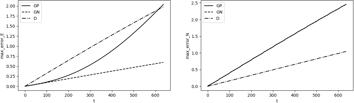
The conservation accuracy of energy in (GP) deteriorates with time, so the error of increases nonlinearly. As a result, (GP) can be less favorable than (D) in long-time experiments. This means that the energy distortion has a negative effect on the (GP) proposed in previous studies. However, our proposed (GN) overcomes this drawback.
4.3.4. Summary of this section
As theoretically shown by Theorem 3.3, the quadratic convergence is numerically demonstrated for many . For the same , there is no significant difference between (D) and (G) in accuracy for and . In terms of execution time, however, (G) is by far superior. Instability due to distortion of conserved quantities corresponding to energy is a concern of (GP), but this issue has been resolved in our proposal (GN). Therefore, as an overall evaluation, (GN) is generally considered superior.
4.4. Experiment 2 : The collision of two solitary waves
Now, we consider a more realistic situation in which two solitary waves collide. In this case, as in the previous studies [5, 16, 9], we consider two solutions that are determined for the same and in the long computational interval . We assume that they have opposite velocities (i.e., one has and the other has ).
In some previous studies, the result for very small is considered as “exact solution” and the errors from the numerical solutions are evaluated. In this study as well, we consider the case for (GN) as the “exact solution”. Since it is difficult to make even smaller due to the execution environment, we treat only .
The major difference from the previous study is that we must also deal with to perform (D), which requires a deeper consideration of the initial conditions.
4.4.1. Initial condition
Let and be a single solitary wave solution that can be written in the form (4.4), (4.5) for some , and , where the solution for moves in the x-axis positive (negative) direction. Then, the initial condition for in this soliton collision experiment is naturally defined as follows:
| (4.7) |
Similar definitions hold for and , which satisfy the periodic boundary condition of the length . However, if we denote for a similarly defined initial condition of , this leads to a contradiction. In other words, holds due to the non-differentiability of .
A way to circumvent this difficulty is to employ corresponding to via the following lemma.
Lemma 4.3.
Another remedy is to consider as the initial condition for .
It is important to note that the initial conditions of and have a significant influence on the results of the numerical experiments. For , let us denote the scheme (G) based on as (), and also (D) based on as (). Under these settings, let us now consider the case where is small, such as , where clearly early convergence can be observed for any method. Then, () and () (and () and ()) converge to similar waveforms, but the results of () and () (and similarly () and ()) are clearly different. This seems natural since the collision problem determined by and is different from that determined by and . In the numerical comparisons, these differences can cause serious confusion, especially when is large and convergence can be expected only for small ’s. There it is hard to know whether the remaining difference (of solutions) comes from the choice of initial data or the difference of schemes. Therefore, in the following, we adopt and , which seem to be more natural initial conditions for the soliton collision experiment. Since it seems mathematically very difficult to obtain an exact analytical solution for the situation where two solitons collide, we does not pursue it in this study.
4.4.2. Result
Now, we show the results when and in Table 3. We denote the error with the “exact solution” as to distinguish it from the case where the error with the true exact solution is evaluated.
| time | |||||||
|---|---|---|---|---|---|---|---|
| 1 | 0.1 | (GP) | 2.59 | 9e-4 | 1.06 | 0.42 | 0.922s |
| (GN) | 2.59 | e-12 | 1.06 | 0.42 | 0.992s | ||
| (D) | 2.59 | e-7 | 0.29 | 0.18 | 10.3s | ||
| 0.05 | (GP) | 2.59 | 1e-4 | 0.28 | 0.10 | 3.40s | |
| (GN) | 2.59 | e-11 | 0.28 | 0.10 | 3.40s | ||
| (D) | 2.59 | e-9 | 0.081 | 0.035 | 43.2s | ||
| 2 | 0.1 | (GP) | 17.44 | 0.042 | 5.58 | 4.42 | 0.687s |
| (GN) | 17.44 | e-11 | 5.59 | 4.42 | 0.604s | ||
| (D) | 17.22 | e-8 | 4.67 | 1.52 | 13.3s | ||
| 0.05 | (GP) | 17.33 | 5e-3 | 1.81 | 0.82 | 2.20s | |
| (GN) | 17.33 | e-10 | 1.79 | 0.82 | 2.13s | ||
| (D) | 17.28 | e-6 | 1.24 | 0.39 | 41.2s | ||
| 0.025 | (GP) | 17.30 | 7e-4 | 0.38 | 0.20 | 8.39s | |
| (GN) | 17.30 | e-9 | 0.38 | 0.20 | 8.64s | ||
| (D) | 17.29 | e-8 | 0.30 | 0.052 | 200s |
The basic trend of the results is the same as in Experiment 1, so (G) is superior for the same reasons as in Experiment 1.
5. Concluding remarks
We have presented a mathematical analysis for the energy-conservative scheme for the Zakharov equations based on DVDM. There we proved solvability under the loosest possible assumptions and improved the argument of convergence by Glassey (the unnecessary condition is removed, at least in the discussion in the convergence estimate). We also reorganized the discussion (borrowed from Glassey’s argument) so that the strategy is more visible. In other words, we now have a better understanding of how to utilize invariants in the analysis of conservative schemes, which we expect can be applied to other schemes.
In addition, the DVDM scheme is compared with Glassey’s scheme by extensive numerical experiments. The results show that (G) outperforms (D) in most situations. This is because the DVDM scheme is merely a consequence of the general method, whereas Glassey’s scheme is an implicit linear scheme cleverly constructed utilizing the properties of the Zakharov equations (and thus faster to solve). However, we also found that if the scheme proposed by Glassey in [10] is implemented as (GP), it becomes unstable in longer experiments due to the distortion of the conserved quantities. This problem is successfully solved by our proposed method of determining .
For future prospects, we are exploring the possibility of applying the structure of the convergence argument to other conservative schemes for other equations, and we are also interested in the other conservative schemes for the Zakharov equations not dealt with in this study. As mentioned in the introduction, the energy-conservative schemes in [5, 11, 15] also all have a distorted form of the invariant corresponding to energy with respect to time. It is a point of concern whether this still implies instability for long-time calculations and whether the issue can be addressed.
Statements and Declarations
There are no conflicts of interests that are related to the content of this study.
References
- [1] Bao, W., Sun, F. and Wei, G.: Numerical methods for the generalized Zakharov system, J. Comput. Phys., 190 (2003), 201–228.
- [2] Bao, W. and Sun, F.: Efficient and stable numerical methods for the generalized and vector Zakharov system, SIAM J. Sci. Comput., 26 (2005), 1057–1088.
- [3] Bhrawy, A. H.: An efficient Jacobi pseudospectral approximation for nonlinear complex generalized Zakharov system, Appl. Math. Comput., 247 (2014), 30–46.
- [4] Bourgain, J. and Colliander, J.: On wellposedness of the Zakharov system, Int. Math. Res. Notices, 11 (1996) 515–546.
- [5] Chang, Q. and Jiang, H.: A conservative difference scheme for the Zakharov equations, J. Comput. Phys., 113.2 (1994), 309–319.
- [6] Colliander, J.: Wellposedness for Zakharov systems with generalized nonlinearity, J. Differ. Equ., 148.2 (1998), 351–363.
- [7] Compaan, E.: A note on global existence for the Zakharov system on , Commun. Pure Appl. Anal., 18.5 (2019), 2473–2489.
- [8] Furihata, D. and Matsuo, T.: Discrete variational derivative method–A structure-preserving numerical method for partial differential equations, CRC Press, Boca Raton, 2011.
- [9] Glassey, R. T.: Approximate solutions to the Zakharov equations via finite differences, J. Comput. Phys., 100.2 (1992), 377–383.
- [10] Glassey, R. T.: Convergence of an energy-preserving scheme for the Zakharov equations in one space dimension. Math. Comput., 58.197 (1992), 83–102.
- [11] Ji, Y. and Ma, H.: Uniform convergence of the Legendre spectral method for the Zakharov equations, Numer. Methods Partial Differ. Equ., 29.2 (2013), 475–495.
- [12] Jin, S. and Zheng, C.: A time-splitting spectral method for the generalized Zakharov system in multi-dimensions, J. Sci. Comput., 26 (2006), 127–149.
- [13] Lees, M.: Energy inequalities for the solution of differential equations, Trans. Amer. Math. Soc., 94 (1960), 58–73.
- [14] Magnus, W., Oberhettinger, F. and Soni, R. P.: Formulas and Theorems for Special Functions of Mathematical Physics, Springer–Verlag, New York, 1966.
- [15] Pan, X. and Zhang, L.: On the convergence of a high-accuracy conservative scheme for the Zakharov equations, Appl. Math. Comput., 297 (2017), 79–91.
- [16] Payne, G. L., Nicholson, D. R. and Downie, R. M.: Numerical solution of the Zakharov equations, J. Comput. Phys., 50.3 (1983), 482–498.
- [17] Sun, Z. Z. and Zhu, Q. D.: On Tsertsvadze’s difference scheme for the Kuramoto-Tsuzuki equation, J. Comput. and Appl. Math., 98.2 (1998), 289–304.
- [18] Wang, J.: Multisymplectic numerical method for the Zakharov system, Comput. Phys. Commun., 180 (2009), 1063–1071.
- [19] Xia, Y., Xu, Y. and Shu, C.W.: Local discontinuous Galerkin methods for the generalized Zakharov system, J. Comput. Phys., 229 (2010), 1238–1259.
- [20] Zakharov, V. E.: Collapse of Langmuir waves, Soviet Phys., JETP, 35 (1972), 908–912.
- [21] Zhou, X. and Zhang, L. M.: A conservative compact difference scheme for the Zakharov equations in one space dimension, Int. J. Comput. Math., 95 (2018), 279–302.