Out-of-time-order correlator as a detector of baryonic phase structure in holographic QCD with a theta angle

Abstract

We study the out-of-time-order correlators (OTOC) of Skyrmion as baryon in the D0-D4/D8 model which is holographically dual to QCD with an non-zero theta angle. The baryon state is identified to the excitation of the Skyrmion which is described by a quantum mechanical system in holography. By employing the definition of OTOC in quantum mechanics, we derive the formulas and demonstrate explicitly the numerical calculations of the OTOC. Our calculation illustrates the quantum OTOC with imaginary Lyapunov coefficient indicates the possibly metastable baryonic status in the presence of the theta angle while the classical OTOC can not, thus it reveals the theta-dependent features of QCD are dominated basically by its quantum properties. Furthermore, the OTOC also implies the baryonic phase becomes really chaotic with real Lyapunov exponent if the theta angle increases sufficiently which agrees with the unstable baryon spectrum presented in this model. In this sense, we believe the OTOC may be treated as a tool to detect the baryonic phase structure of QCD.

Si-wen Li, Yi-peng Zhang, Hao-qian Li,

1 Introduction

In recent years, the out-of-time-order correlator (OTOC) has been considered as a measure of the magnitude of quantum chaos [1] while it was first introduced to calculate the vertex correction of a current for a superconductor [2]. In general, the quantum OTOC $C_{T}\left(t\right)$ is defined by using the commutator of two operators as,

$$C_{T}=-\left\langle\left[W\left(t\right),V\left(0\right)\right]^{2}\right\rangle,$$ (1.1)

where $W\left(t\right),V\left(t\right)$ are operators in the Heisenberg picture at time $t$ and $\left\langle...\right\rangle$ refers to the thermal average. In particular, the authors of [3, 4, 5] suggest that the operators $W\left(t\right),V\left(t\right)$ in quantum mechanics can be chosen as the canonical coordinate $x\left(t\right)$ and momentum $p\left(t\right)$. In this sense, the classical limit of the OTOC can also be evaluated quantitatively if the quantum commutator $\frac{1}{i}\left[,\right]$ is replaced by the Poisson bracket $\left\{,\right\}_{\mathrm{P.B}}$. Accordingly, the chaos of classically mechanical system can be evaluated through the OTOC as,

$$C_{T}\sim\left\{x\left(t\right),p\left(0\right)\right\}_{\mathrm{P.B}}^{2}\sim\left[\frac{\delta x\left(t\right)}{\delta x\left(0\right)}\right]^{2}\sim e^{2Lt},$$ (1.2)

where $L$ is the Lyapunov coefficient. For a chaotic system, $L$ must be positive since such a system is very sensitive to the initial condition $x\left(0\right)$ otherwise it is not really chaotic. However, the quantum version of the OTOC (1.2) could instead saturate at the Ehrenfest time $t_{E}$ which refers to a time scale that the wave function spreads over the whole system characterizing the boundary between the particle-like and the wave-like behavior of a wave function. Therefore, the exponent growth of the OTOC is conjectured to be the characteristic property of the classical system.

Moreover, the OTOC is also an important observable in the context of quantum gravity, AdS/CFT correspondence or gauge-gravity duality [6, 7]. In the context of quantum information on the horizon of black hole [8, 9, 10, 11, 12, 13], it implies an upper bound of the quantum Lyapunov coefficient as $L\leq 2\pi T$. On the other hand, the analysis of chaos in the Sachdev-Ye-Kitaev (SYK) model [14, 15] (a quantum mechanical system with infinitely long range disorder interactions of Majorana fermions) illustrates the bound of quantum Lyapunov exponent is saturated [16, 17, 18]. Therefore, it strongly implies a quantum black hole can be described by the SYK model in holography if the OTOC could be a tool to detect the AdS/CFT correspondence or gauge-gravity duality.

Motivated by these, in this work we would like to introduce OTOC as a tool to detect the baryonic phase structure of QCD in holography, in order to further explore the role of OTOC in gauge-gravity duality. To this goal, we aim at the D0-D4/D8 model [19, 20, 21, 22] as an extension of the famous D4/D8 model (Witten-Sakai-Sugimoto model) [23, 24, 25, 26, 27] based on the IIA string theory which is holographically dual to theta-dependent QCD. The reasons to choose the D0-D4/D8 model are given as follows: First, the baryon sector in this model is a quantum mechanical system which is totally analytical and simple enough in the strong coupling region, hence the definition of OTOC in quantum mechanics is valid. Second, the baryon sector in the presence of a non-vanished theta angle would include various phase structures in this model [28, 29]. Therefore we expect the OTOC may somehow detect the these phase structures by Lyapunov exponent in holography. Keep these in hand, our calculation illustrates that the quantum OTOC does not grow exponentially when the theta angle is sufficiently small, instead it trends to become oscillated periodically in the large $N_{c}$ limit, and the period increases by the theta angle. So if we write the OTOC as an imaginary exponent as it is suggested in [4], the Lyapunov coefficient indicates the possible baryonic status with non-zero theta angle in QCD which is recognized to be metastable in this model [21, 22, 28, 29]. However, the analysis of the classical OTOC does not lead to this conclusion sensibly. Besides, our analysis also implies the real Lyapunov exponent may arise in the OTOC at large time when the theta angle increase greatly, therefore it implies the baryonic phase becomes unstable and chaotic with sufficiently large theta angle. In this sense, the holographic OTOC as a tool seems possible to detect the baryonic phase structure of QCD and implies the features of QCD in the presence of the theta angle is dominated basically by the quantum properties of the theory.

The outline of this paper is as follows. In Section 2, we collect the essential parts of the Skyrmion as baryon in the D0-D4/D8 model as a quantum mechanical system, then derive briefly the formulas of the OTOC. In Section 3, we illustrate our numerical evaluation of the OTOCs with various parameters and analyze their behaviors. In Section 4, the classical limit of the OTOCs is discussed. The final section as Section 5 gives the summary. In addition, the appendix includes some essential calculations in this work.

2 The holographic setup

2.1 The holographic Skyrmion in the D0-D4/D8 model

The D0-D4/D8 model is a top-down holographic approach to QCD with a non-vanished theta angle which is also an extension of the D4/D8 model (the Witten-Sakai-Sugimoto model) [23, 24, 25, 26, 27]. The Skyrmion as baryon in this model is recognized as the collective mode of a baryon vertex which is a D4-brane wrapped on the spherical part $S^{4}$ of the bulk geometry [37, 38] and it can be equivalently described by the instanton configuration of the gauge field on the flavor brane [39, 40, 41]. By evaluating the mass of the instantonic soliton on the flavor brane, the quantized Hamiltonian in moduli space for Skyrmion as baryon in the D0-D4/D8 model is collected as [28],

$$H= M_{0}+H_{Z}+H_{y},$$

$$H_{Z}= -\frac{1}{2m_{Z}}\partial_{Z}^{2}+\frac{1}{2}m_{Z}\omega_{Z}^{2}Z^{2},$$

$$H_{y}= -\frac{1}{2m_{\rho}}\sum_{I=1}^{n+1}\frac{\partial^{2}}{\partial y_{I}^{2}}+\frac{1}{2}m_{\rho}\omega_{\rho}^{2}\rho^{2}+\frac{K}{m_{\rho}\rho^{2}},$$ (2.1)

where $a=\frac{1}{216\pi^{3}}$ and

$$M_{0}= 8\pi^{2}\lambda ab^{3/2}N_{c},m_{Z}=\frac{1}{2}m_{\rho}=8\pi^{2}ab^{3/2}N_{c},$$

$$\omega_{Z}^{2}= \frac{1}{3}\left(3-b\right),\omega_{\rho}^{2}=\frac{1}{12}\left(3-b\right),K=\frac{2}{5}N_{c}^{2}.$$ (2.2)

Here $N_{c},N_{f}$ refers respectively to the color and flavor number (i.e. numbers of D4-branes and D8-branes). $\lambda$ is the ’t Hooft coupling constant. $b$ relates to the number density of the D0-branes, and for a given branch, $b$ also relates to the theta angle of QCD in holography by [20, 21, 22, 42],

$$\theta\propto\sqrt{\frac{b-1}{b}}.$$ (2.3)

Thus we have $1\leq b<3$ which implies the baryonic phase is possible to be stable when the theta angle is sufficiently small since $b>3$ means $\omega_{Z},\omega_{\rho}$ are all imaginary so that the Skyrmion as baryon is totally unstable. $n$ relates to the flavor number $N_{f}$ of the Skyrmion through the numbers of the $SU\left(N_{f}\right)$ generators as $n=N_{f}^{2}-1$. We note that the above formulas are written in the unit of $M_{KK}=1$. $\rho$ refers to the size of the instanton which denotes the radial coordinate in the moduli space parameterized by $y_{I}$ as $\rho^{2}=\sum_{I}y_{I}^{2}$.

The eigen equation with respect to Hamiltonian (2.1) as,

$$H\psi=E\psi,$$ (2.4)

can be solved analytically. The associated eigenfunction $\psi$ is given as,

$$\psi_{n_{Z},n_{\rho},l_{n},l_{n-1},...l_{1}}\left(Z,\rho,\theta_{n},\theta_{n-1},...\theta_{1}\right)=\chi_{n_{Z}}\left(Z\right)\mathcal{R}_{n_{\rho},l_{n}}\left(\rho\right)\mathcal{Y}\left(\theta_{n},\theta_{n-1},...\theta_{1}\right),$$ (2.5)

where

$$\mathcal{R}_{n_{\rho},l_{n}}\left(\rho\right) =\mathcal{N}\left(n_{\rho},l_{n}\right)e^{-\frac{m_{\rho}\omega_{\rho}\rho^{2}}{2}}\rho^{\xi}F\left(-n_{\rho},\xi+\frac{n+1}{2},m_{\rho}\omega_{\rho}\rho^{2}\right),$$

$$\xi =\sqrt{2K+\left(l_{n}+\frac{n-1}{2}\right)^{2}}-\frac{n-1}{2},$$ (2.6)

is given by the confluent hypergeometric function $F\left(a,b,x\right)$ satisfying the normalization

$$\int d\rho\rho^{n}\mathcal{R}_{n_{\rho}^{\prime},l_{n}^{\prime}}\mathcal{R}_{n_{\rho},l_{n}}=\delta_{n_{\rho}^{\prime},n_{\rho}}.$$ (2.7)

And

$$\mathcal{Y}\left(\theta_{n},\theta_{n-1},...\theta_{1}\right)=\frac{\left(-1\right)^{l_{1}}}{\sqrt{2\pi}}e^{il_{1}\theta_{1}}\prod_{j=2}^{n}\ {}_{j}\mathcal{P}_{l_{j}}^{l_{j-1}}\left(\theta_{j}\right),$$ (2.8)

is the spherical harmonic function on $S^{n}$. We note that $\ {}_{j}\mathcal{P}_{l_{j}}^{l_{j-1}}\left(\theta_{j}\right)$ is given by combining the associated Legendre polynomial $P_{l}^{m}\left(\cos\theta\right)$ as [43],

$$\ \ \ \ \ \ \ \ \ \ \ \ \ {}_{j}\mathcal{P}_{l_{j}}^{l_{j-1}}\left(\theta_{j}\right)=\sqrt{\frac{2l_{j}+j-1}{2}\frac{\left(l_{j}+l_{j-1}+j-2\right)!}{\left(l_{j}-l_{j-1}\right)!}}\sin^{\frac{2-j}{2}}\theta_{j}P_{l_{j}+\frac{j-2}{2}}^{-\left(l_{j-1}+\frac{j-2}{2}\right)}\left(\cos\theta_{j}\right).$$ (2.9)

Thus the spherical harmonic function $\mathcal{Y}\left(\theta_{n},\theta_{n-1},...\theta_{1}\right)$ satisfies the eigen equation,

$$\nabla_{S^{n}}^{2}\mathcal{Y}_{l_{n},l_{n-1},...l_{1}}\left(\theta_{n},\theta_{n-1},...\theta_{1}\right)=-l_{n}\left(l_{n}+n-1\right)\mathcal{Y}_{l_{n},l_{n-1},...l_{1}}\left(\theta_{n},\theta_{n-1},...\theta_{1}\right),$$ (2.10)

and the normalization condition

$$\int\mathcal{Y}_{l_{n}^{\prime},l_{n-1}^{\prime},...l_{1}^{\prime}}^{*}\mathcal{Y}_{l_{n},l_{n-1},...l_{1}}dV_{S^{n}}=\prod_{j=1}^{n}\delta_{l_{j}^{\prime}l_{j}}.$$ (2.11)

$\chi_{n_{Z}}\left(Z\right)$ represents the eigenfunction of $H_{Z}$ which is obviously the eigenfunction of one-dimensional harmonic oscillator. Keeping these in hand, the eigenvalue of Hamiltonian (2.1) is obtained as,

$$E_{n_{Z},n_{\rho},l_{n}}\left(N_{c},n\right)=E_{n_{Z}}+E_{n_{\rho},l_{n}}\left(N_{c},n\right)+M_{0},$$ (2.12)

where

$$E_{n_{Z}}=\left(n_{Z}+\frac{1}{2}\right)\omega_{Z},\ E_{n_{\rho},l_{n}}\left(N_{c},n\right)=\left[\sqrt{2K+\left(l_{n}+\frac{n-1}{2}\right)^{2}}+2n_{\rho}+1\right]\omega_{\rho}.$$ (2.13)

2.2 The formula of QTOC in quantum mechanics

In quantum mechanics, [3, 4, 5] suggest the thermal and microcanonical OTOC $C_{T},c_{n}$ can be defined respectively as,

$$C_{T}\left(t\right)=\frac{1}{\mathcal{Z}}\sum_{n}e^{-\beta E_{n}}c_{n}\left(t\right),\ \mathcal{Z}=\sum_{n}e^{-\beta E_{n}},\ c_{n}\left(t\right)=-\left\langle n\left|\left[x\left(t\right),p\right]^{2}\right|n\right\rangle,$$ (2.14)

for a time-independent Hamiltonian $H\left(x_{1},x_{2}...x_{J},p_{1},p_{2}...p_{J}\right)$. Here $\mathcal{Z}$ is the partition function, $\beta=1/T$ refers to the temperature of the system, $\left|n\right\rangle$ refers to the $n$-th eigenstate of Hamiltonian satisfying the eigen equation $H\left|n\right\rangle=E_{n}\left|n\right\rangle$ and $x\left(t\right),p\left(t\right)$ is respectively the canonical coordinate and momentum in Heisenberg picture. Let us denote the canonical coordinate and momentum as,

$$x\left(t\right)=x_{a}\left(t\right),p\left(t\right)=p_{a}\left(t\right),p=p\left(0\right),a\in\left\{1,2...J\right\},$$ (2.15)

for notational simplicity. Using the completeness condition in quantum mechanics, the OTOC can be written as,

$$c_{n}\left(t\right)=-\sum_{m}\left\langle n\left|\left[x\left(t\right),p\right]\right|m\right\rangle\left\langle m\left|\left[x\left(t\right),p\right]\right|n\right\rangle\equiv\sum_{m}b_{nm}\left(t\right)b_{nm}^{*}\left(t\right),$$ (2.16)

where

$$b_{nm}\left(t\right)=-i\left\langle n\left|\left[x\left(t\right),p\right]\right|m\right\rangle.$$ (2.17)

Recall the unitary transformation $x\left(t\right)=e^{iHt}xe^{-iHt}$, (2.16) can be further rewritten as,

$$b_{nm}\left(t\right)=-i\sum_{k}\left(e^{iE_{nk}t}x_{nk}p_{km}-e^{iE_{km}t}p_{nk}x_{km}\right),$$ (2.18)

where $x_{nk}=\left\langle n\left|x\right|k\right\rangle,p_{nk}=\left\langle n\left|p\right|k\right\rangle$ and $E_{nk}=E_{n}-E_{k}$. If a time-independent Hamiltonian is given as,

$$H=\sum_{a=1}^{J}\frac{p_{a}^{2}}{2m_{X}}+U\left(x_{1},x_{2}...x_{J}\right),$$ (2.19)

the following relation can be obtained as,

$$p_{mn}=im_{X}E_{mn}x_{mn},$$ (2.20)

by the commutation relation $\left[H,x\right]=-\frac{ip}{m_{X}}$ which leads to

$$b_{nm}\left(t\right)=m_{X}\sum_{k}x_{nk}x_{km}\left(E_{km}e^{iE_{nk}t}-E_{nk}e^{iE_{km}t}\right).$$ (2.21)

Therefore the OTOCs can be obtained by using (2.14) (2.16) and (2.21). We note that since $H_{Z}$ presented in (2.1) is nothing but the Hamiltonian of one-dimensional harmonic oscillator, it OTOC can be analytically obtained as [3, 4],

$$C_{T}\left(t\right)=c_{n_{Z}}\left(t\right)=m_{Z}^{2}\cos^{2}\omega_{Z}t.$$ (2.22)

Accordingly, in the following discussion, we will focus on the numerical evaluation of the OTOCs with respect to $H_{y}$.

3 The numerical analysis

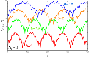
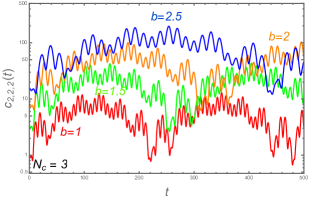
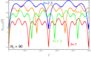
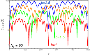
Figure 1: The two-flavored ($N_{f}=2$) microcanonical OTOCs $c_{n_{\rho},l_{3},l_{2}}$ ($c_{0,0,0},c_{2,2,2}$) as functions of time $t$ with various $b$.

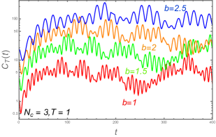
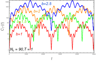
Figure 2: The two-flavored ($N_{f}=2$) thermal OTOCs $C_{T}$ as functions of time $t$ with various $b$.

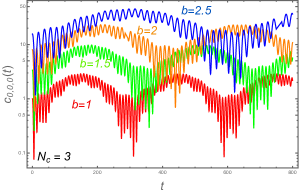
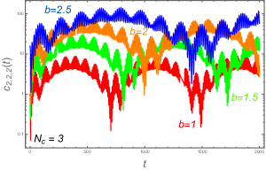
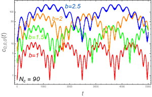
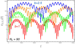
Figure 3: The three-flavored ($N_{f}=3$) microcanonical OTOCs $c_{n_{\rho},l_{8},l_{7}}$ ($c_{0,0,0},c_{2,2,2}$) as functions of time $t$ with various $b$.

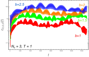
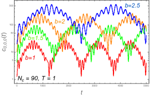
Figure 4: The three-flavored ($N_{f}=3$) thermal OTOCs $C_{T}$ as functions of time $t$ with various $b$.

The microcanonical and thermal OTOCs $c_{n_{\rho},l_{n},l_{n-1}...l_{1}}\left(t\right),C_{T}\left(t\right)$ of the holographic Skyrmion with various $b$ are given in Figure 1 - 4. We note that the quantum numbers $l_{n-2},l_{n-3},...l_{2},l_{1}$ are degenerated quantum numbers, thus we denote $c_{n_{\rho},l_{n},l_{n-1}...l_{1}}\left(t\right)$ as $c_{n_{\rho},l_{n},l_{n-1}}\left(t\right)$. The sum presented in (2.16) and (2.21) has been truncated at $n_{c}=4$ i.e. $0\leq n_{Z},n_{\rho},l_{n}\leq n_{c}$ for the actual numerical calculation and the degeneracy number $n_{\mathrm{d}}$ in $c_{n_{\rho},l_{n},l_{n-1}...l_{1}}\left(t\right)$ is computed as,

$$n_{\mathrm{d}}\left(l_{n}\right)=\sum_{l_{n-1}=0}^{l_{n}}\sum_{l_{n-2}=0}^{l_{n-1}}...\sum_{l_{3}=0}^{l_{4}}\sum_{l_{2}=0}^{l_{3}}\left(2l_{2}+1\right).$$ (3.1)

Thus it includes totally $\left(n_{c}+1\right)^{2}\times\sum_{l_{3}=0}^{n_{c}}n_{\mathrm{d}}\left(l_{3}\right)=1375$ states for $N_{f}=2$ and $\left(n_{c}+1\right)^{2}\times\sum_{l_{8}=0}^{n_{c}}n_{\mathrm{d}}\left(l_{8}\right)=16500$ states for $N_{f}=3$ contributing to the OTOC. Our numerical calculation reveals the following features of the OTOC. First, the thermal OTOCs do not display the apparent exponential growth while they grow at early times. Thus the exponential growth expected in the classical OTOC is not apparent which supports the exponential growth of OTOC is the character for a classical mechanical system only. Second, the microcanonical OTOCs are approximately periodic because of the commensurable energy spectrum. For the situation $N_{c}\gg 1$, the period $\Delta t$ of microcanonical OTOCs is evaluated as $\Delta t\sim\mathrm{min}\left[E_{n_{\rho},l_{n};n_{\rho}^{\prime},l_{n}^{\prime}}^{-1}\right]\sim N_{c}$ for $N_{c}\rightarrow\infty$ which displays the large-$N_{c}$ behaviors of the microcanonical OTOCs as [4]. Third, the thermal OTOCs grow with $b$ i.e. the presence of the theta angle according to (2.3) and in addition they tend to become periodic at large $N_{c}$ as the microcanonical OTOCs.

Keep these in hand, let us attempt to outline how to use OTOC of the holographic Skyrmion to describe the various status of the baryonic phase with various $b$ in this model. As the OTOC is periodic for large $N_{c}$, it means the quantum mechanical system (2.1) is not really chaotic. Nevertheless, we can define imaginary Lyapunov coefficient $L$ as it is suggested in [4] to characterize the periodic quantum OTOC $C_{T}$ as $C_{T}\left(t\right)\sim e^{iLt}$. Therefore, according to the numerical calculation presented in Figure 1 - 4, we can see that imaginary Lyapunov coefficient $L$ decreases with the growth of $b$. On the other hand, the holographic Skyrmion in the D0-D4/D8 system is recognized as baryon state [27, 28, 29, 40, 41], it means $L\left(b\right)$ as an order parameter indicates possibly baryonic states with various $b$ or theta angle. Recall the holographic description of the metastable baryonic states in [28, 29], it seemingly implies the value of $L$ with $b>1$ represents the metastable baryonic states and $b=1$ represents the baryonic states become stable. So the Lyapunov coefficient as a function of theta angle indicates the metastability or stability of the baryonic phase, just as the Lyapunov coefficient $L$ is a parameter characterizing the chaos.

Moreover, although the Hamiltonian for Skyrmion (2.1) is strictly valid only for $1\leq b\leq 3$, it would be interesting to extend our discussion with $b>3$. According to (2.2) (2.12) and (2.21), the energy difference $E_{nk}$ becomes totally imaginary if $b>3$, so the OTOC contains the factor $e^{\left|E_{nk}\right|t}$ i.e. the real Lyapunov exponent. While this may not be very obvious for the OTOC of the $y$ part, it is easy to see by recalling the $Z$ part OTOC given in (2.22). For $b>3$, $\omega_{Z}$ is purely imaginary so that we have $C_{T}\sim\cos^{2}\omega_{Z}t\rightarrow e^{2\left|\omega_{Z}\right|t}$ at large $t$ and this behavior of OTOC implies the Lyapunov exponent becomes real and the system becomes really chaotic. This is reasonable since the harmonic oscillator with imaginary frequency is totally unstable and very sensitive to its initial state. Altogether, we can see the imaginary Lyapunov coefficient indicates the metastability or stability of the baryonic phase while the real Lyapunov coefficient indicates its instability. In this sense, we may conclude that the Lyapunov coefficient could be treated as an order parameter to indicate the baryonic phase structure.

4 The classical limit of the OTOC

According to the definition (2.14), the classical version of OTOC can be naturally obtained by replacing the quantum commutators with Poisson bracket, i.e. $\frac{1}{i}\left[,\right]\rightarrow\left\{,\right\}_{\mathrm{P.B}}$. And thermal average must be replaced by the integral in the phase space consisted of canonical coordinate $\mathbf{q}$ and momentum $\mathbf{p}$. Therefore, we can obtain the classical version of the OTOC presented in (2.14) as,

$$C_{T}^{\mathrm{cl}}\left(t\right)=\frac{1}{\mathcal{Z}_{\mathrm{cl}}}\int\frac{d\mathbf{q}d\mathbf{p}}{\left(2\pi\right)^{n+2}}e^{-\beta H}\left\{\mathbf{q}\left(t\right),\mathbf{p}\left(0\right)\right\}_{\mathrm{P.B}}^{2},c^{\mathrm{cl}}\left(t\right)=\left\{\mathbf{q}\left(t\right),\mathbf{p}\left(0\right)\right\}_{\mathrm{P.B}}^{2},$$ (4.1)

where

$$\mathcal{Z}_{\mathrm{cl}}=\int\frac{d\mathbf{q}d\mathbf{p}}{\left(2\pi\right)^{n+2}}e^{-\beta H}.$$ (4.2)

Besides, the classical version of the Hamiltonian (2.1) of the Skyrmion is given by

$$H= M_{0}+H_{Z}+H_{y},$$

$$H_{Z}= \frac{p_{Z}^{2}}{2m_{Z}}+\frac{1}{2}m_{Z}\omega_{Z}^{2}Z^{2},$$

$$H_{y}= \frac{1}{2m_{\rho}}\sum_{I=1}^{n+1}p_{I}^{2}+\frac{1}{2}m_{\rho}\omega_{\rho}^{2}\rho^{2}+\frac{K}{m_{\rho}\rho^{2}}.$$ (4.3)

As the canonical coordinate $\mathbf{q}$ and momentum $\mathbf{p}$ is chosen as $\mathbf{q}=\left\{Z,y_{I}\right\},\mathbf{p}=\left\{p_{Z},p_{I}\right\}$, for the $Z$ part in Hamiltonian (4.3), its classical solution is given as,

$$Z\left(t\right) =Z\cos\omega_{Z}t+\frac{p_{Z}}{m_{Z}}\sin\omega_{Z}t,$$

$$p_{Z}\left(t\right) =-m_{Z}\omega_{Z}\sin\omega_{Z}t+p_{Z}\omega_{Z}\cos\omega_{Z}t.$$ (4.4)

Hence the associated OTOCs are computed as,

$$c_{n_{Z}}^{\mathrm{cl}}\left(t\right) =\left\{Z\left(t\right),p_{Z}\left(0\right)\right\}_{\mathrm{P.B}}^{2}=\left[\frac{\delta Z\left(t\right)}{\delta Z\left(0\right)}\right]^{2}=\cos^{2}\omega_{Z}t,$$

$$C_{T}^{\mathrm{cl}}\left(t\right) =\frac{1}{\mathcal{Z}_{\mathrm{cl}}}\int\frac{d\mathbf{q}d\mathbf{p}}{\left(2\pi\right)^{n+2}}e^{-\beta H}\left\{Z\left(t\right),p_{Z}\left(0\right)\right\}_{\mathrm{P.B}}^{2}=\cos^{2}\omega_{Z}t,$$ (4.5)

which agrees quantitatively with its quantum version. For the $y$ part in (4.3), the classical equation of motion is obtained as,

$$m_{\rho}\ddot{y}_{I}=\left(-m_{\rho}\omega_{\rho}^{2}+\frac{2K}{m_{\rho}\rho^{4}}\right)y_{I}.$$ (4.6)

Note that for the classical Skyrmion, $\rho$ refers to the size of the Skyrmion (as instantons) which must minimize the classical Hamiltonian (4.3), thus we have [28]

$$\rho^{\mathrm{cl}}=\frac{\left(2K\right)^{1/4}}{\left(m_{\rho}\omega_{\rho}\right)^{1/2}}.$$ (4.7)

Impose (4.7) into (4.6), the classical solution for $y_{I}$ is

$$y_{I}\left(t\right)=y_{I}\left(0\right)+\frac{p_{I}\left(0\right)}{m_{\rho}}t,$$ (4.8)

then the associated OTOCs are calculated as,

$$c_{y_{I}}^{\mathrm{cl}} =\left\{y_{I}\left(t\right),p_{I}\left(0\right)\right\}_{\mathrm{P.B}}^{2}=1,$$

$$C_{T}^{\mathrm{cl}}\left(t\right) =\frac{1}{\mathcal{Z}_{\mathrm{cl}}}\int\frac{d\mathbf{q}d\mathbf{p}}{\left(2\pi\right)^{n+2}}e^{-\beta H}\left\{y_{I}\left(t\right),p_{I}\left(0\right)\right\}_{\mathrm{P.B}}^{2}=1,$$ (4.9)

which does not display the apparent dependence on $b$ different from the quantum OTOCs. In this sense, we comment that if the Lyapunov coefficient could be an order parameter to characterize some properties of QCD, it implies the theta-dependence is basically dominated by the quantum feature of QCD, as it should be [36].

5 Summary

In this work, we employ the definition of OTOC in quantum mechanics to derive the formulas and demonstrate explicitly the numerical calculations of the OTOC of the holographic Skyrmion in the D0-D4/D8 model which is equivalent to the theta-dependent QCD according to the gauge-gravity duality. Our numerical calculation supports that exponential growth of the OTOC is the character of the classical chaotic system [3, 4, 5] and shows that OTOCs increase in the presence of the theta angle. In addition, we attempt to use the imaginary Lyapunov coefficient as an order parameter to indicate the various status of the baryonic phase which illustrates the possibly metastable states of baryon as it is discussed in the existing works [21, 28, 29]. Although the quantum OTOCs with imaginary Lyapunov exponent reveals the spreadability of the baryonic wave function instead of the chaos of the system, it displays that the baryonic status with maximum Lyapunov coefficient (i.e. vanished theta angle) is stable according to the discussion in [21, 28, 29]. Moreover, we also attempt to extend our analysis with sufficiently large theta angle. In this case, the baryonic phase becomes unstable which leads to real Lyapunov exponent in OTOC at large time. So it seems the Lyapunov coefficient as an order parameter in OTOC may detect some properties of the QCD phase structure somehow. Besides, we evaluate the classical limit of the OTOC whose behavior is quite different from its quantum version. In particular, the theta-dependence is less clear in the $y$ part of the classical OTOC which may imply that the theta-dependence basically comes from the quantum features of QCD. Therefore, this work suggests that we can use OTOC as a tool to detect the features of QCD phase structure.

Appendix: The calculation of matrix element in the OTOC

In this appendix, we will outline the calculation of matrix element $x_{mn}$ (2.21) presented in the OTOC. As the Hamiltonian $H_{y}$ in (2.1) for the Skyrmion is defined in $n+1$ dimensional moduli space, let us start with the $n+1$ dimensional Euclidean space $\mathbb{R}^{n+1}$ parametrized by $y_{I}=\left\{y_{1},y_{2},...y_{n+1}\right\}$ as the Cartesian coordinates. Since $H_{y}$ only depends on the radial coordinates $\rho$ in the moduli space, we consider the spherical coordinates $\left\{\rho,\theta_{1},...,\theta_{n-1},\theta_{n}\right\}$ with the following coordinate transformation

$$y_{I}=\rho\cos\theta_{I-1}\prod_{J=I}^{n}\sin\theta_{j},\ \rho^{2}=\sum_{I=1}^{n+1}y_{I}^{2},$$ (A-1)

where $\theta_{0}=0$. Thus the Euclidean metric on $\mathbb{R}^{n+1}$ is given as,

$$ds^{2}=\delta_{IJ}dy_{I}dy_{J}=d\rho^{2}+\rho^{2}d\Omega_{n}^{2},$$ (A-2)

where $d\Omega_{n}^{2}$ represents the angular differential on a unit $S^{n}$ satisfying the recurrence relation,

$$d\Omega_{n}^{2}=d\theta_{n}^{2}+\sin^{2}\theta_{n}d\Omega_{n-1}^{2}.$$ (A-3)

Therefore, $d\Omega_{n}^{2}$ can be rewritten as,

$$d\Omega_{n}^{2}=\sum_{I=1}^{n}\left(d\theta_{I}^{2}\prod_{J=I+1}^{n}\sin^{2}\theta_{J}\right),$$ (A-4)

and the volume element $dV_{n+1}$ of $\mathbb{R}^{n+1}$ reads as

$$dV_{n+1} =\sqrt{g}d\rho d\theta_{n}d\theta_{n-1}...d\theta_{1}=\rho^{n}d\rho\prod_{J=1}^{n}\sin^{J-1}\theta_{J}d\theta_{J}\equiv\rho^{n}d\rho dV_{S^{n}}.$$ (A-5)

Recall the spherical harmonic function $\mathcal{Y}_{l_{n},l_{n-1},...l_{1}}\left(\theta_{n},\theta_{n-1},...\theta_{1}\right)$ on $S^{n}$ given in (2.8), one can verify $\mathcal{Y}_{l_{n},l_{n-1},...l_{1}}\left(\theta_{n},\theta_{n-1},...\theta_{1}\right)$ is the eigenfunction of Laplacian operator $\nabla_{S^{n}}^{2}$ satisfying

$$\nabla_{S^{n}}^{2}\mathcal{Y}_{l_{n},l_{n-1},...l_{1}}\left(\theta_{n},\theta_{n-1},...\theta_{1}\right)=-l_{n}\left(l_{n}+n-1\right)\mathcal{Y}_{l_{n},l_{n-1},...l_{1}}\left(\theta_{n},\theta_{n-1},...\theta_{1}\right),$$ (A-6)

where the quantum number satisfies $\left|l_{1}\right|\leq l_{2}\leq l_{3}\leq...l_{n}.$ We note that the Laplacian operator $\nabla_{S^{n}}^{2}$ satisfies the following recurrence as,

$$\nabla_{S^{n+1}}^{2}=\sin^{-n}\theta_{n+1}\frac{\partial}{\partial\theta_{n+1}}\sin^{n}\theta_{n+1}\frac{\partial}{\partial\theta_{n+1}}+\sin^{-2}\theta_{n+1}\nabla_{S^{n}}^{2},$$ (A-7)

where $\theta_{n+1}$ is the $n+1$-th spherical coordinate on $S^{n+1}$. Thus, use the identity for the associated Legendre polynomial $P_{l}^{m}\left(\cos\theta\right)$

$$\frac{l+m}{2l+1}P_{l-1}^{m}\left(\cos\theta\right)+\frac{l-m+1}{2l+1}P_{l+1}^{m}\left(\cos\theta\right)=\cos\theta P_{l}^{m}\left(\cos\theta\right),$$ (A-8)

after some messy but straightforward calculations, we can obtain

$$\cos\theta_{n}\mathcal{Y}_{l_{n},l_{n-1},...l_{1}}= \sqrt{\frac{\left(l_{n}-l_{n-1}\right)\left(l_{n}+l_{n-1}+n-2\right)}{\left(2l_{n}+n-1\right)\left(2l_{n}+n-3\right)}}\mathcal{Y}_{l_{n}-1,l_{n-1},...l_{1}}$$

$$+\sqrt{\frac{\left(l_{n}+l_{n-1}+n-1\right)}{\left(2l_{n}+n-1\right)}\frac{\left(l_{n}-l_{n-1}+1\right)}{\left(2l_{n}+n+1\right)}}\mathcal{Y}_{l_{n}+1,l_{n-1},...l_{1}},$$ (A-9)

which leads to a useful integration,

$$Y_{l_{n}^{\prime},l_{n-1}^{\prime},...l_{1}^{\prime};l_{n},l_{n-1},...l_{1}}\equiv \int dV_{S^{n}}\mathcal{Y}_{l_{n}^{\prime},l_{n-1}^{\prime},...l_{1}^{\prime}}^{*}\cos\theta_{n}\mathcal{Y}_{l_{n},l_{n-1},...l_{1}}$$

$$= \bigg{[}\sqrt{\frac{\left(l_{n}-l_{n-1}\right)\left(l_{n}+l_{n-1}+n-2\right)}{\left(2l_{n}+n-1\right)\left(2l_{n}+n-3\right)}}\delta_{l_{n}^{\prime},l_{n}-1}$$

$$+\sqrt{\frac{\left(l_{n}+l_{n-1}+n-1\right)}{\left(2l_{n}+n-1\right)}\frac{\left(l_{n}-l_{n-1}+1\right)}{\left(2l_{n}+n+1\right)}}\delta_{l_{n}^{\prime},l_{n}+1}\bigg{]}\times\prod_{j=1}^{n-1}\delta_{l_{j}^{\prime},l_{j}}.$$ (A-10)

Keep these in hand, let us choose one of the coordinates $y_{I}=\left\{y_{1},y_{2},...y_{n+1}\right\}$ to compute its matrix element $\left\langle n_{Z},n_{\rho},l_{n},l_{n-1},...l_{1}\left|y_{I}\right|n_{Z}^{\prime},n_{\rho}^{\prime},l_{n}^{\prime},l_{n-1}^{\prime},...l_{1}^{\prime}\right\rangle$. Due to the spherical symmetry in the Hamiltonian (2.1), we can choose the $n+1$-th coordinate $y_{n+1}=\rho\cos\theta_{n}$ for simplification. Note that although we use one quantum number $\left|m\right\rangle$ to denote the eigenstate of the Hamiltonian presented in (2.1), we must keep in mind the eigenstate is denoted by multiple quantum numbers $n_{Z},n_{\rho},l_{n},l_{n-1},...l_{1}$ according to (2.5). Hence we can write explicitly the matrix element $x_{mk}$ presented in (2.21) as,

$$x_{mk}= \left\langle n_{Z},n_{\rho},l_{n},l_{n-1},...l_{1}\left|y_{n+1}\right|n_{Z}^{\prime},n_{\rho}^{\prime},l_{n}^{\prime},l_{n-1}^{\prime},...l_{1}^{\prime}\right\rangle$$

$$= \left\langle n_{Z},n_{\rho},l_{n},l_{n-1},...l_{1}\left|\rho\cos\theta_{n}\right|n_{Z}^{\prime},n_{\rho}^{\prime},l_{n}^{\prime},l_{n-1}^{\prime},...l_{1}^{\prime}\right\rangle$$

$$= \delta_{n_{Z}^{\prime},n_{Z}}\rho_{n_{\rho}^{\prime},l_{n}^{\prime};n_{\rho},l_{n}}Y_{l_{n}^{\prime},l_{n-1}^{\prime},...l_{1}^{\prime};l_{n},l_{n-1},...l_{1}},$$ (A-11)

where we have used the normalization of the wave function given in (2.5) and (A-10) with

$$\rho_{n_{\rho}^{\prime},l_{n}^{\prime};n_{\rho},l_{n}}=\int\rho^{n+1}d\rho\mathcal{R}_{n_{\rho}^{\prime},l_{n}^{\prime}}\mathcal{R}_{n_{\rho},l_{n}}.$$ (A-12)

By defining the kernels of the useful functions as,

$$Y_{l_{n}^{\prime},l_{n-1}^{\prime},...l_{1}^{\prime};l_{n},l_{n-1},...l_{1}}= Y_{l_{n}^{\prime},l_{n-1}^{\prime};l_{n},l_{n-1}}^{\mathrm{ker}}\delta_{n_{Z}^{\prime},n_{Z}}\prod_{j=1}^{n-2}\delta_{l_{j}^{\prime},l_{j}},$$

$$x_{n_{\rho}^{\prime},l_{n}^{\prime},l_{n-1}^{\prime};n_{\rho},l_{n},l_{n-1}}^{\mathrm{ker}}= \rho_{n_{\rho}^{\prime},l_{n}^{\prime};n_{\rho},l_{n}}Y_{l_{n}^{\prime},l_{n-1}^{\prime};l_{n},l_{n-1}}^{\mathrm{ker}},$$

$$Y_{l_{n}^{\prime},l_{n-1}^{\prime};l_{n},l_{n-1}}^{\mathrm{ker}}= \bigg{[}\sqrt{\frac{\left(l_{n}-l_{n-1}\right)\left(l_{n}+l_{n-1}+n-2\right)}{\left(2l_{n}+n-1\right)\left(2l_{n}+n-3\right)}}\delta_{l_{n}^{\prime},l_{n}-1}$$

$$+\sqrt{\frac{\left(l_{n}+l_{n-1}+n-1\right)}{\left(2l_{n}+n-1\right)}\frac{\left(l_{n}-l_{n-1}+1\right)}{\left(2l_{n}+n+1\right)}}\delta_{l_{n}^{\prime},l_{n}+1}\bigg{]}\delta_{l_{n-1}^{\prime},l_{n-1}},$$ (A-13)

the matrix element $b_{nm}$ defined in (2.21) can be written explicitly as,

$$b_{n_{Z},n_{\rho},l_{n},l_{n-1},...l_{1};n_{Z}^{\prime},n_{\rho}^{\prime},l_{n}^{\prime},l_{n-1}^{\prime},...l_{1}^{\prime}}\left(t\right)$$

$$= m_{\rho}\sum_{n_{\rho}^{\prime\prime},l_{n}^{\prime\prime},l_{n-1}^{\prime\prime}}\delta_{n_{Z},n_{Z}^{\prime}}x_{n_{\rho},l_{n},l_{n-1};n_{\rho}^{\prime\prime},l_{n}^{\prime\prime},l_{n-1}^{\prime\prime}}^{\mathrm{ker}}x_{n_{\rho}^{\prime\prime},l_{n}^{\prime\prime},l_{n-1}^{\prime\prime};n_{\rho}^{\prime},l_{n}^{\prime},l_{n-1}^{\prime}}^{\mathrm{ker}}\prod_{j=1}^{n-2}\delta_{l_{j},l_{j}^{\prime}}$$

$$\times\bigg{(}E_{n_{Z}^{\prime},n_{\rho}^{\prime\prime},l_{n}^{\prime\prime};n_{Z}^{\prime},n_{\rho}^{\prime},l_{n}^{\prime}}e^{iE_{n_{Z},n_{\rho},l_{n};n_{Z}^{\prime},n_{\rho}^{\prime\prime},l_{n}^{\prime\prime}}t}-E_{n_{Z},n_{\rho},l_{n};n_{Z}^{\prime},n_{\rho}^{\prime\prime},l_{n}^{\prime\prime}}e^{iE_{n_{Z}^{\prime},n_{\rho}^{\prime\prime},l_{n}^{\prime\prime};n_{Z}^{\prime},n_{\rho}^{\prime},l_{n}^{\prime}}t}\bigg{)},$$ (A-14)

where $E_{n_{Z},n_{\rho},l_{n};n_{Z}^{\prime},n_{\rho}^{\prime},l_{n}^{\prime}}$ refers to the difference of the energy defined by (2.12) (2.13) with various quantum numbers $n_{Z},n_{\rho},l_{n};n_{Z}^{\prime},n_{\rho}^{\prime},l_{n}^{\prime}$. Therefore the microcanonical OTOC $c_{n}\left(t\right)$ can be written as,

$$c_{n_{Z},n_{\rho},l_{n},l_{n-1},...l_{1}}\left(t\right)$$

$$= \sum_{n_{Z}^{\prime},n_{\rho}^{\prime},l_{n}^{\prime},l_{n-1}^{\prime},...l_{1}^{\prime}}b_{n_{Z},n_{\rho},l_{n},l_{n-1},...l_{1};n_{Z}^{\prime},n_{\rho}^{\prime},l_{n}^{\prime},l_{n-1}^{\prime},...l_{1}^{\prime}}^{*}b_{n_{Z},n_{\rho},l_{n},l_{n-1},...l_{1};n_{Z}^{\prime},n_{\rho}^{\prime},l_{n}^{\prime},l_{n-1}^{\prime},...l_{1}^{\prime}}$$

$$= m_{\rho}^{2}\sum_{n_{\rho}^{\prime},l_{n}^{\prime},l_{n-1}^{\prime};n_{\rho}^{\prime\prime},l_{n}^{\prime\prime},l_{n-1}^{\prime\prime};n_{\rho}^{\prime\prime\prime},l_{n}^{\prime\prime\prime},l_{n-1}^{\prime\prime\prime}}$$

$$\bigg{[}x_{n_{\rho},l_{n},l_{n-1};n_{\rho}^{\prime\prime},l_{n}^{\prime\prime},l_{n-1}^{\prime\prime}}^{\mathrm{ker}}x_{n_{\rho}^{\prime\prime},l_{n}^{\prime\prime},l_{n-1}^{\prime\prime};n_{\rho}^{\prime},l_{n}^{\prime},l_{n-1}^{\prime}}^{\mathrm{ker}}x_{n_{\rho},l_{n},l_{n-1};n_{\rho}^{\prime\prime\prime},l_{n}^{\prime\prime\prime},l_{n-1}^{\prime\prime\prime}}^{\mathrm{ker}}x_{n_{\rho}^{\prime\prime\prime},l_{n}^{\prime\prime\prime},l_{n-1}^{\prime\prime\prime};n_{\rho}^{\prime},l_{n}^{\prime},l_{n-1}^{\prime}}^{\mathrm{ker}}$$

$$\times\bigg{(}E_{n_{\rho}^{\prime\prime},l_{n}^{\prime\prime};n_{\rho}^{\prime},l_{n}^{\prime}}e^{-iE_{n_{\rho},l_{n};n_{\rho}^{\prime\prime},l_{n}^{\prime\prime}}t}-E_{n_{\rho},l_{n};n_{\rho}^{\prime\prime},l_{n}^{\prime\prime}}e^{-iE_{n_{\rho}^{\prime\prime},l_{n}^{\prime\prime};n_{\rho}^{\prime},l_{n}^{\prime}}t}\bigg{)}$$

$$\times\bigg{(}E_{n_{\rho}^{\prime\prime\prime},l_{n}^{\prime\prime\prime};n_{\rho}^{\prime},l_{n}^{\prime}}e^{iE_{n_{\rho},l_{n};n_{\rho}^{\prime\prime\prime},l_{n}^{\prime\prime\prime}}t}-E_{n_{\rho},l_{n};n_{\rho}^{\prime\prime\prime},l_{n}^{\prime\prime\prime}}e^{iE_{n_{\rho}^{\prime\prime\prime},l_{n}^{\prime\prime\prime};n_{\rho}^{\prime},l_{n}^{\prime}}t}\bigg{)}\bigg{]},$$ (A-15)

where

$$E_{n_{Z},n_{\rho},l_{n};n_{Z},n_{\rho}^{\prime},l_{n}^{\prime}}\equiv E_{n_{\rho},l_{n}}-E_{n_{\rho}^{\prime},l_{n}^{\prime}}=E_{n_{\rho},l_{n};n_{\rho}^{\prime},l_{n}^{\prime}}.$$ (A-16)

Altogether, the OTOC is able to be evaluated numerically once the kernel of the matrix elements $x_{n_{\rho}^{\prime\prime},l_{n}^{\prime\prime},l_{n-1}^{\prime\prime};n_{\rho}^{\prime},l_{n}^{\prime},l_{n-1}^{\prime}}^{\mathrm{ker}}$ is obtained. In addition, the thermal OTOC can be obtained by using (2.14) as,

$$C_{T}\left(t\right)=\frac{1}{\mathcal{Z}}\sum_{n_{Z},n_{\rho},l_{n},l_{n-1}...l_{1}}c_{n_{Z},n_{\rho},l_{n},l_{n-1},...l_{1}}\left(t\right)e^{-\frac{E_{n_{Z},n_{\rho},l_{n}}}{T}},$$ (A-17)

where the partition function is given by

$$\mathcal{Z}=\sum_{n_{Z},n_{\rho},l_{n},l_{n-1}...l_{1}}e^{-\frac{E_{n_{Z},n_{\rho},l_{n}}}{T}}=\sum_{n_{Z},n_{\rho},l_{n}}n_{\mathrm{d}}e^{-\frac{E_{n_{Z},n_{\rho},l_{n}}}{T}},$$ (A-18)

and $n_{\mathrm{d}}$ is the degeneracy number in (3.1) for a given energy $E_{n_{Z},n_{\rho},l_{n}}$.

References

• [1] J. Maldacena, S Shenke, D. Stanford, “A bound on chaos”, JHEP 08 (2016) 106, arXiv:1503.01409.
• [2] A. Larkin, Y. Ovchinnikov, “Quasiclassical method in the theory of superconductivity”, J. Exp. Theor. Phys. 28, 1200–1205 (1969).
• [3] K. Hashimoto, K. Murata, R.Yoshii, “Out-of-time-order correlators in quantum mechanics”, JHEP 10 (2017) 138, arXiv:1703.09435.
• [4] K. Hashimoto, K. Murata, K.Yoshida, “Chaos in chiral condensates in gauge theories”, Phys.Rev.Lett. 117 (2016) 23, 231602, arXiv:1605.08124.
• [5] T. Akutagawa, K. Hashimoto, T. Sasaki, R. Watanabe, “Out-of-time-order correlator in coupled harmonic oscillators”, JHEP 08 (2020) 013, arXiv:2004.04381.
• [6] J. Maldacena, “The Large N limit of superconformal field theories and supergravity”, Adv.Theor.Math.Phys. 2 (1998) 231-252, arXiv:hep-th/9711200.
• [7] O. Aharony, S. Gubser, J. Maldacena, H. Ooguri, Y. Oz, “Large N field theories, string theory and gravity”, Phys. Rept. 323 (2000) 183, arXiv:hep-th/9905111.
• [8] S. Shenker, D. Stanford, “Black holes and the butterfly effect”, JHEP 03 (2014) 067, arXiv:1306.0622.
• [9] S. Shenker, D. Stanford, “Multiple Shocks”, JHEP 12 (2014) 046, arXiv:1312.3296.
• [10] S. Leichenauer, “Disrupting Entanglement of Black Holes”, Phys.Rev.D 90 (2014) 4, 046009, arXiv:1405.7365.
• [11] S. H. Shenker, D. Stanford, “Stringy effects in scrambling”, JHEP 05 (2015) 132, arXiv:1412.6087.
• [12] S. Jackson, L. McGough, H. Verlinde, “Conformal Bootstrap, Universality and Gravitational Scattering”, Nucl.Phys.B 901 (2015) 382-42, arXiv:1412.5205.
• [13] J. Polchinski, “Chaos in the black hole S-matrix”, arXiv:1505.08108.
• [14] S. Sachdev, J. Ye, “Gapless spin fluid ground state in a random, quantum Heisenberg magnet”, Phys.Rev.Lett. 70 (1993) 3339, arXiv:cond-mat/9212030.
• [15] A. Kitaev, talks given at KITP, April and May 2015.
• [16] D. J. Gross, V. Rosenhaus, “A Generalization of Sachdev-Ye-Kitaev”, JHEP 02 (2017) 093, arXiv:1610.01569.
• [17] E. Witten, “An SYK-Like Model Without Disorder”, J.Phys.A 52 (2019) 47, 474002, arXIv:1610.09758.
• [18] T. Nishinaka, S. Terashima, “A note on Sachdev–Ye–Kitaev like model without random coupling”, Nucl.Phys.B 926 (2018) 321-334, arXiv:1611.10290.
• [19] K. Suzuki, D0 - D4 system and QCD(3+1), Phys.Rev.D 63 (2001) 084011, arXiv:hep-th/0001057.
• [20] S. Seki, S. Sin, “A New Model of Holographic QCD and Chiral Condensate in Dense Matter”, JHEP 10 (2013) 223 , arXiv:1304.7097.
• [21] L. Bartolini, F. Bigazzi, S. Bolognesi, A. Cotrone, A. Manenti, “Theta dependence in Holographic QCD”, JHEP 02 (2017) 029, arXiv:1611.00048.
• [22] C. Wu, Z. Xiao, D. Zhou, “Sakai-Sugimoto model in D0-D4 background”, Phys.Rev.D 88 (2013) 2, 026016 , arXiv:1304.2111.
• [23] T. Sakai, S. Sugimoto, “Low energy hadron physics in holographic QCD”, Prog.Theor.Phys. 113 (2005) 843-882 , arXiv:hep-th/0412141.
• [24] E. Witten, “Anti-de Sitter Space, Thermal Phase Transition, And Confinement In Gauge Theories”, Adv.Theor.Math.Phys. 2 (1998) 505-532, arXiv:hep-th/9803131.
• [25] T. Sakai, S. Sugimoto, “More on a holographic dual of QCD”, Prog.Theor.Phys. 114 (2005) 1083-1118, arXiv:hep-th/0507073.
• [26] E. Kiritsis, “String theory in a nutshell”, Princeton University Press (2019).
• [27] S. Li, X. Zhang, “The D4/D8 Model and Holographic QCD”, Symmetry 15 (2023) 6, 1213, arXiv:2304.10826.
• [28] W. Cai, C. Wu, Z. Xiao, “Baryons in the Sakai-Sugimoto model in the D0-D4 background”, Phys.Rev.D 90 (2014) 10, 106001, arXiv:1410.5549.
• [29] S. Li, T. Jia, “Matrix model and Holographic Baryons in the D0-D4 background”, Phys.Rev.D 92 (2015) 4, 046007, arXiv:1506.00068.
• [30] M. D’Elia, F. Negro, “Theta dependence of the deconfinement temperature in Yang-Mills theories”, Phys.Rev.Lett. 109 (2012) 072001, arXiv:1205.0538.
• [31] M. D’Elia, F. Negro, “Phase diagram of Yang-Mills theories in the presence of a theta term”, Phys.Rev.D 88 (2013) 3, 034503, arXiv:1306.2919.
• [32] L. Debbio, G. Manca, H. Panagopoulos, A. Skouroupathis, E. Vicari, “Theta-dependence of the spectrum of SU(N) gauge theories”, JHEP 06 (2006) 005, arXiv:hep-th/0603041.
• [33] E. Witten, “Theta Dependence In The Large N Limit Of Four-Dimensional Gauge Theories”, Phys.Rev.Lett. 81 (1998) 2862-2865, arXiv:hep-th/9807109.
• [34] K. Buckley, T. Fugleberg, A. Zhitnitsky, “Can Induced Theta Vacua be Created in Heavy Ion Collisions?”, Phys.Rev.Lett. 84 (2000) 4814-4817, arXiv:hep-ph/9910229.
• [35] STAR Collaboration, “Search for the chiral magnetic effect with isobar collisions at $\sqrt{s_{NN}}=200$ ” by the STAR Collaboration at the BNL Relativistic Heavy Ion Collider, Phys.Rev.C 105 (2022) 1, 014901, arXiv:2109.00131.
• [36] E. Vicari, H. Panagopoulos, “Theta dependence of SU(N) gauge theories in the presence of a topological term”, Phys.Rept. 470 (2009) 93-150, arXiv:0803.1593.
• [37] E. Witten, “Baryons And Branes In Anti de Sitter Space”, JHEP 07 (1998) 006, arXiv:hep-th/9805112.
• [38] D. Gross, H. Ooguri, “Aspects of Large N Gauge Theory Dynamics as Seen by String Theory”, Phys.Rev.D 58 (1998) 106002, arXiv:hep-th/9805129.
• [39] D. Tong, “TASI lectures on solitons: Instantons, monopoles, vortices and kinks”, TASI 2005, arXiv:hep-th/0509216.
• [40] H. Hata, T. Sakai, S. Sugimoto, S. Yamato, “Baryons from instantons in holographic QCD”, Prog.Theor.Phys. 117 (2007) 1157, arXiv:hep-th/0701280.
• [41] H. Hata, M.Murata, “Baryons and the Chern-Simons term in holographic QCD with three flavors”, Prog.Theor.Phys. 119 (2008) 461-490, arXiv:0710.2579.
• [42] Si-wen Li, Hao-qian Li, Yi-peng Zhang, “The worldvolume fermion as baryon in holographic QCD with a theta angle”, arXiv:2402.01197.
• [43] Si-wen Li, Yi-peng Zhang, Hao-qian Li, “Out-of-time-order correlators of Skyrmion as baryon in holographic QCD”, arXiv:2401.04421.