Discrete-Time Modeling and Handover Analysis of Intelligent Reflecting Surface-Assisted Networks

Abstract

Owning to the reflection gain and double path loss featured by intelligent reflecting surface (IRS) channels, handover (HO) locations become irregular and the signal strength fluctuates sharply with variations in IRS connections during HO, the risk of HO failures (HOFs) is exacerbated and thus HO parameters require reconfiguration. However, existing HO models only assume monotonic negative exponential path loss and cannot obtain sound HO parameters. This paper proposes a discrete-time model to explicitly track the HO process with variations in IRS connections, where IRS connections and HO process are discretized as finite states by measurement intervals, and transitions between states are modeled as stochastic processes. Specifically, to capture signal fluctuations during HO, IRS connection state-dependent distributions of the user-IRS distance are modified by the correlation between measurement intervals. In addition, states of the HO process are formed with Time-to-Trigger and HO margin whose transition probabilities are integrated concerning all IRS connection states. Trigger location distributions and probabilities of HO, HOF, and ping-pong (PP) are obtained by tracing user HO states. Results show IRSs mitigate PPs by 48% but exacerbate HOFs by 90% under regular parameters. Optimal parameters are mined ensuring probabilities of HOF and PP are both less than 0.1%.

I Introduction

Intelligent reflecting surface (IRS) has emerged as a promising solution to cope with the ever-growing demands of capacity through the new concept of reconfiguring the wireless propagation environment [1]. However, passive reflection gains cause handover (HO) locations to shift irregularly [2] and double path loss (also termed multiplicative fading) causes the signal strength to drop steeply during user movement [3], which poses challenges to HO performance.

Through targeted reflective beamforming, an IRS with $N$ reflective units can boost the signal from the serving base station (BS) by $O(N^{2})$. Meanwhile, signals from neighboring BSs are not specifically adjusted because no IRS is scheduled for them [4], which creates distinct channel gains and shifts in the HO locations. HO locations become irregular because IRSs are deployed in a distributed manner [5, 6], which brings the risks of unreasonable HO decisions and challenges to theoretical modeling. Another feature of the IRS channel is double path loss, which causes a significant drop in signal strength with user movement [7]. Signal degradation during the HO process exacerbates the risk of handover failure (HOF) [10]. Moreover, the gain of the IRS cascaded channel varies nonlinearly with geometric relations among IRS, BS, and user, with the additional aspect of dynamical IRS reselection [2], the signal strength becomes a stochastic process during HO owing to random IRS connections. Consequently, changes in HO locations and signal strength fluctuations make HO parameters commonly used inapplicable, and an analytical HO model is desired for sound HO parameter settings and IRS configurations. Although many analytical models have been proposed for coverage performance (e.g.,[8] and [9]), the analysis of HO performance in IRS-assisted networks is still in its infancy.

I-A Related Works

Stochastic geometry has been extensively used to analyze HO performance metrics. The HO trigger locations are sets of points equidistant from BSs in single-tier terrestrial networks [11, 12] and single-tier drone-aided networks [13] due to the same transmission power. However, unlike the serving BS, the reference signals from neighboring BSs are not boosted via the IRS due to no schedule [4], which results in differential channel gains of BSs. Thus, a closer BS may not provide a stronger signal and the HO locations shift as the IRS enhances the serving signal, whereas the distance-based HO models in [11, 12, 13] are not applicable to IRS-assisted networks.

Since the user equipment (UE)-BS Euclidean distance is not sufficient to determine HO locations, equivalent analysis techniques [14, 15] and analytical geometric frameworks [16, 17] have been proposed to obtain the number of HO triggers in heterogeneous networks. However, the IRS channel gains vary with the geometric relations of the IRS, BS, and UE, instead of linearly adjusting the signal strength and only considering the relative locations of UE and BS. However, the analyses in [14, 15, 16, 17] are limited to the analysis of the number of HO triggers; the actual HO process is not addressed.

Among the HO events A1 to A6, the A3 event is the most focused on by scholars because only the A3 event assesses a relative comparison between the signal quality of the serving cell and that of neighboring cells [18]. The HO process with A3 event involves HO parameters of Time-to-Trigger (TTT) and hysteresis threshold parameters, which are used to avoid unnecessary HOs (also known as the ping-pong (PP) effect); thus, the models in [11, 12, 13, 14, 15, 16, 17, 30] overestimate the number of actual HO executions. The sojourn time is analyzed in [19] and [20] to evaluate PPs. However, in addition to the PPs caused by early HO decisions, a postponed HO decision may cause a low signal-to-interference (SIR) ratio, resulting in HOFs [21]. For analyzing both the PP effect and HOF, the exact HO trigger location, SIR changes within the TTT duration, and the user’s cell sojourn time must be analyzed.

To obtain the optimal HO parameters, HO models for HOF and PP analyses have been proposed for single-tier [22, 23] and heterogeneous [24, 26, 25, 27, 28] networks without IRSs. For IRS-assisted networks, the minimization of HOs is formed as an optimization problem in [29] rather than as an analytical model. [30] performed a preliminary analysis to obtain only HO probabilities. Many unexplored problems remain regarding the establishment of an analytical model for the HO process in IRS-assisted networks.

• The IRS channel gain with user movement has not been tracked theoretically. Negative exponential path-loss is adopted in [23, 24, 26, 25] to characterize the signal strength fluctuation. However, IRS reselections cause randomness. The signal strength was modified by independent fluctuations in [22, 27, 28]. However, the relative location of the user to the IRS between measurement moments is correlated. IRS channels were introduced into HO probability analysis in [30]. Nevertheless, [30] only evaluated whether an HO is triggered within a unit time, thus lacking IRS channel gain modeling during HO.

• Current HO models have not introduced the effect of IRS implementation on the HO process. Locations of HOF and PP are modeled as circular boundaries in [23, 24, 26, 25, 27, 28], enabling HO process analysis. However, distributed IRSs make locations of HO events irregular, thus circular boundary models are ineffective. The transitions between HO states are modeled explicitly in [22]. Nevertheless, owing to the lack of considering IRS reflection gains, the HO state transitions in [22] are not applicable for the HO process in IRS-assisted networks.

• Existing works cannot obtain reference-worthy results for HO in IRS-assisted networks. Lacking analysis of signal strength fluctuation and HO state transitions with IRS, models in [22, 23, 24, 26, 25, 27, 28] are inaccurate in indicating actual HO performance and guiding HO parameters for IRS-assisted networks. Simulation-based and analytical model-based HO probabilities with IRS are given in [29] and [30]. Nevertheless, HO probabilities alone cannot represent the mobility performance, creating an urgent need to analyze both HOF and PP, and it is difficult to obtain guidelines via the computationally intensive simulation in [29].

I-B Contribution

This paper proposes a discrete-time model to explicitly model signal strength fluctuations, enabling the HO analysis of IRS-assisted networks, where processes of IRS connection and HO are defined as finite states and tracked without information loss. The main contributions are summarized as follows.

• The signal strength fluctuation during HO under the IRS cascaded channel is tracked theoretically. As the process of IRS connection is defined in the state space of the discrete-time model, the geometric relation between the HO user and its serving IRS is tracked. The probability density function (pdf) of IRS-user distance is revised via the correlation between measurement intervals to obtain the IRS reflection gain along the user trajectory.

• The HO state transitions during the HO process are modified by IRS reflection gains. The processes for HO events (HO, HOF, and PP) occurring are described based on the actual timing relationships of the HO process and HO parameters. IRS reflection gains are introduced into transition probability matrices of HO states to analyze the exact HO trigger location, SIR changes within TTT duration, and user sojourn time.

• Critical HO performance metrics for IRS-assisted networks are deduced. HO state vectors are constituted by probabilities of HO states. HO state vectors along the user trajectory are obtained based on the discrete-time model of the IRS connection and HO process. Compact expressions of HOF and PP probability are deduced by extracting elements of the HO state vectors, and the trigger location distributions of HO events are obtained.

• Design insights obtained from the main results include: (i) The IRS implementation provides a new tradeoff for HOF and PP, where IRSs mitigate the PP probability by 48% but exacerbate the HOF probability by 90% when the density of IRS is 500/km², and the element number is 100; (ii) Guidance for the setting of HO parameters (TTT and HO margin) is studied, optimal HO parameters are mined to make the probability of PP and HOF both less than 0.1% under multiple network setups.

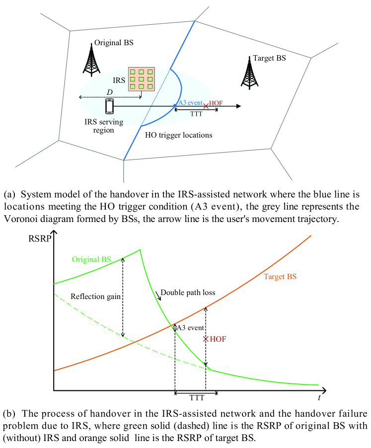
Figure 1: Handover process in the IRS-assisted networks: (a) The IRS-assisted network structure; (b) The received signal strength changes with time.

II System Model

II-A Network Model

In this paper, we consider an IRS-assisted multi-cell wireless network, as shown in Fig 1(a), where BSs are distributed according to a 2D homogenous Poisson point process (HPPP) with density $\lambda_{b}$ and the same transmitting power $P_{t}$, denoted as $\Phi_{b}$. IRSs are each equipped with $N$ reflecting elements to assist the user-BS communications, which are distributed according to another 2D HPPP with density $\lambda_{r}$, denoted as $\Phi_{r}$ [7]. The BS controls the IRSs in its cell, i.e., each IRS is controlled by its nearest BS [5]. A limited IRS serving distance is considered, which is denoted by $D$, because the IRS provides signal enhancement via reflecting beamforming in a local region [7, 31].

According to 3GPP specifications [18], the UE performs channel measurements periodically, and the measurement interval is defined as $T_{d}$. Owing to the filtering process at UE, the effect of the fast-fading of the channel is averaged out [23, 24, 26, 25]. The path-loss model proposed in [7] is adopted to capture the reflection gain of the BS-IRS-user link. For the BS to which the user is connected, its signal is enhanced by the IRS (if it exists); thus, the received signal strength is given by

$${{\cal S}^{c}}\!\!\left({{x},{d}}\right)=\left\{\begin{array}[]{ll}{P_{t}}{\Gamma_{bf}}\left({{d}}\right){g_{b}}\left({{x}}\right),&{d}\leq D\\ {P_{t}}{g_{b}}\left({{x}}\right),&{d}>D\end{array}\right.,$$ (1)

where $x$ and $d$ denote the distance between the user and the BS connected and the distance between the user and the serving IRS, respectively, $g_{b}{\left(x\right)}=\beta{x^{-\alpha}}$, ${\alpha}$ denotes the path-loss exponent, $\beta={\left({{{4\pi{f_{c}}}\mathord{\left/{\vphantom{{4\pi{f_{c}}}c}}\right.\kern-1.2pt}c}}\right)^{-2}}$, $f_{c}$ is the carrier frequency, $c$ denotes the speed of light. ${\Gamma_{bf}}\left(d\right)$ indicates the additional gain from the IRS reflection, which is given by

$${\Gamma_{bf}}({d}) =1+{G_{bf}}{g_{r}}({d})+N\frac{\pi}{4}\sqrt{\pi{g_{r}}({d})},$$ (2)

where $g_{r}{\left(d\right)}=\beta{d^{-\alpha}}$, ${G_{bf}}=\frac{{{\pi^{2}}}}{{16}}{N^{2}}+\left({1-\frac{{{\pi^{2}}}}{{16}}}\right)N$.

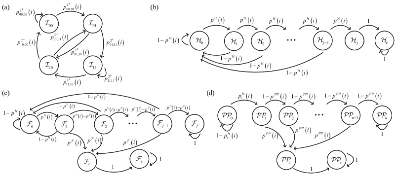
Figure 2: Discrete-time models for (a) IRS connections, (b) handover, (c) handover failure, and (d) ping-pong. The symbols of each state are inside the circles and the state transition probabilities are beside the lines.

For the neighboring BS, because no IRS reflecting beamforming is provided for the measured reference signal [7, 30], the received signal strength is ${{\cal S}^{n}}\!\!\left({{x}}\right)={P_{t}}{g_{b}}\left({{x}}\right)$.

II-B IRS Connection Events

In IRS-assisted networks, the BS dynamically schedules the best IRS for the user to perform the service (if any IRSs of that cell exists within a distance $D$ from the user) based on the measurement [7, 30, 31]. Therefore, the following IRS connection events are considered.

Initial connection to IRS: The user not served by the IRS steps into the serving region of an IRS of the serving cell. Alternatively, the user handovers to a new cell and connects to its available IRS of the new cell.

Disconnection of IRS: The user leaves its IRS serving region and there is no IRS within $D$ of the serving cell. Alternatively, the user handovers to a new cell and disconnects it from the IRS of the original cell.

Reselection: When there is an IRS of the serving cell that is closer to the user than the serving IRS, the BS schedules that IRS to serve the user.

II-C Handover Process and Events

As shown in Fig. 1(b), the HO process involves the following steps:

HO triggering: As only the A3 event assesses a comparison between the signal of the serving cell and that of neighbor cells [18], the condition of the A3 event is considered as the HO trigger condition in this paper, which is also considered in [22, 23, 24, 26, 25, 27, 28]. Specifically, HO is triggered when the RSS of the target BS is more than the hysteresis threshold ${\gamma_{\rm{HO}}}$ stronger than the serving BS.

TTT Timing: When the condition of the A3 event is satisfied, the TTT timer starts, which is set to avoid unnecessary HOs.

HO execution: Only when the condition of the A3 event is satisfied in the entire TTT duration, the UE feeds back the measurement report to the serving BS and waits for the HO command to perform subsequent steps. Therefore, the condition for HO execution can be expressed as

$$\frac{{{{\cal S}^{n}}\!\!\left({{x_{t}}}\right)}}{{{{\cal S}^{c}}\!\!\left({{x_{o}},{d}}\right)}}>{\gamma_{{\rm{HO}}}},\forall t\in\left[{{t_{0}},{t_{0}}+{T_{t}}}\right],$$ (3)

where $x_{o}$ and $x_{t}$ indicate the distances from the user to the original BS and target BS, respectively, ${\gamma_{{\rm{HO}}}}$ is the HO margin, $t_{0}$ is the moment when the HO trigger condition is satisfied.

To evaluate the HO performance, the following two events are of most interest:

HOF: A drop in wideband SIR to a threshold results in the inability to receive HO commands, i.e., HOF [18]. As [22, 23, 24, 26, 25, 27, 28], an interference-limited system is considered, along with the interference from the target BS, which is the absolute main part. Thus, the condition of HOF is given by

$$\frac{{{{\cal S}^{c}}\!\!\left({{x_{o}},{d}}\right)}}{{{{\cal S}^{n}}\!\!\left({{x_{t}}}\right)}}<{Q_{out}},\exists t\in\left[{{t_{0}},{t_{0}}+{T_{t}}}\right].$$ (4)

where $Q_{out}$ denotes the threshold for HOF.

PP: The occurrence of PP depends on the user sojourn time in the new cell. If the user handovers to a new BS and handovers back to the original BS within a certain time threshold, the HO is considered unnecessary, which is defined as a PP. After HO, the user disconnects from the original BS and is connected to the target BS. Thus, a PP occurs when conditions (3) and (5) are satisfied, and (5) is given by

$$\frac{{{{\cal S}^{n}}\!\!\left({{x_{o}}}\right)}}{{{{\cal S}^{c}}\!\!\left({{x_{t}},{d}}\right)}}>{\gamma_{{\rm{HO}}}},\exists t\in\left[{{t_{0}}+{T_{t}},{t_{0}}+{T_{p}}}\right],$$ (5)

where $T_{p}$ denotes the minimum threshold for the sojourn time.

II-D User Mobility

Without loss of generality, a typical user is considered to move at a constant speed $v$ and direction during the entire HO process, which is the same as the assumptions in [22, 23, 24, 26, 25, 27, 28]. The straight line along which the user trajectory is located is denoted by $l_{u}$. The BSs involved in the HO process are considered, which are the original BS and the target BS. The locations of the original BS and target BS are denoted as $b_{o}$ and $b_{t}$. The vertical lines from $b_{o}$ and $b_{t}$ are considered as the straight line $l_{u}$, and the foot points are denoted as $b^{\prime}_{o}$ and $b^{\prime}_{t}$, respectively. The distance between the original BS (target BS) and the straight line $l_{u}$ is denoted as $r_{o}$ ($r_{t}$); in particular, $r_{t}$ takes a negative value when BSs are located on both sides of $l_{u}$, that is, $r_{t}=-\left|{{b_{t}}{b’_{t}}}\right|$. As in [22, 23], we focus on the part of the user trajectory that starts with $b’_{o}$ and ends with $b’_{t}$. The distance between $b’_{o}$ and $b’_{t}$ is denoted as $L$, whose probability density function (pdf) is given by [32]

$${f_{L}}\left(l\right)=\int\limits_{0}^{\pi}{\int\limits_{0}^{\pi}{\frac{{{\pi^{2}}\lambda_{b}^{\frac{3}{2}}{l^{2}}{\rho_{\upsilon}}{\rho_{\tau}}\left({2\pi{\lambda_{b}}{l^{2}}b_{0}^{2}\rho_{\upsilon}^{2}-{c_{0}}}\right)}}{{\sin\left({\upsilon+\tau}\right)}}}}$$ (6)

$$\times\exp\left({-\pi{\lambda_{b}}{l^{2}}{V_{2}}\left({\upsilon,\tau}\right)}\right){\rm{d}}\upsilon{\rm{d}}\tau,$$

where ${\rho_{\upsilon}}=\frac{{\sin\upsilon}}{{\sin\left({\upsilon+\tau}\right)}}$, ${\rho_{\tau}}=\frac{{\sin\tau}}{{\sin\left({\upsilon+\tau}\right)}}$, ${V_{2}}\left({\upsilon,\tau}\right)=\left({1+\rho_{\tau}^{2}-2{\rho_{\tau}}\cos\upsilon}\right)\left({1-\frac{\tau}{\pi}+\frac{{\sin 2\tau}}{{2\pi}}}\right)+\rho_{\tau}^{2}\left({1-\frac{\upsilon}{\pi}+\frac{{\sin 2\upsilon}}{{2\pi}}}\right)$, ${b_{0}}=\frac{{\left({\pi-\tau}\right)\cos\tau+\sin\tau}}{\pi}$, and ${c_{0}}=\frac{{\left({\pi-\tau}\right)+\sin\tau\cos\tau}}{\pi}$.

III Discrete-Time Models for IRS Connections and Handover

III-A IRS Connections

To track the signal strength fluctuations along the user trajectory theoretically, a discrete-time model of the IRS connection is established, as shown in Fig. 2(a). The user trajectory is discretized based on the measurement interval $T_{d}$; thus, the user moves ${\Delta x}={T_{d}}\cdot v$ in each measurement interval. Four IRS connection states are defined: ${\mathcal{I}}^{k}_{00}$, ${\mathcal{I}}^{k}_{01}$, ${\mathcal{I}}^{k}_{10}$, and ${\mathcal{I}}^{k}_{11}$. The first digit (0 or 1) of the subscript represents the user’s IRS connection for the previous measurement moment, the second digit of the subscript indicates the status for the current measurement moment, 0 indicates that the user is not being served by the IRS, and 1 indicates that an IRS serves the user. $k\in\left\{{o,t}\right\}$ represents the IRS connection state of IRSs controlled by the original BS or the target BS. The correlation between measurement intervals is introduced as the IRS connection at the previous measurement moment is always regarded. Therefore, the specific definitions of the four IRS connection states are as follows:

1. No connection to IRS: the user is not served by any IRSs in both moments, which is indicated by ${\mathcal{I}}^{k}_{00}$.

2. Initial connection to IRS: same as that described in Section II.B, which is indicated by ${\mathcal{I}}^{k}_{01}$.

3. Disconnection of IRS: same as that described in Section II.B, which is indicated by ${\mathcal{I}}^{k}_{10}$.

4. Keeping the connection to IRS: the user is consistently served by an IRS at two moments or the user is served by a closer IRS (i.e., reselection described in Section II.B), which is indicated by ${\mathcal{I}}^{k}_{11}$.

Based on the definitions of the IRS connection states, the corresponding state transition matrix and state vector are constructed as follows:

Lemma 1

The state transition matrix of the IRS connection is given by

$$\small{{\rm{\bf{T}}}^{{\mathcal{I}}^{k}}}\!\!\!\left(i\right)\!=\!\left[{\begin{array}[]{*{20}{c}}{p_{00,00}^{{{\mathcal{I}}^{k}}}\left(i\right)}&{p_{00,01}^{{{\mathcal{I}}^{k}}}\left(i\right)}&0&0\\ 0&0&{p_{01,10}^{{{\mathcal{I}}^{k}}}\left(i\right)}&{p_{01,11}^{{{\mathcal{I}}^{k}}}\left(i\right)}\\ {p_{10,00}^{{{\mathcal{I}}^{k}}}\left(i\right)}&{p_{10,01}^{{{\mathcal{I}}^{k}}}\left(i\right)}&0&0\\ 0&0&{p_{11,10}^{{{\mathcal{I}}^{k}}}\left(i\right)}&{p_{11,11}^{{{\mathcal{I}}^{k}}}\left(i\right)}\end{array}}\right],$$ (7)

where ${p_{m,n}^{{{\mathcal{I}}^{k}}}\left(i\right)},k\in\left\{{o,t}\right\},m,n\in\left\{{00,01,10,11}\right\}$ is state transition probabilities of IRS connection sates, which are given in (8) and (9) (at the bottom of the next page).

Proof:

See Appendix A. ∎

$$p_{00,00}^{{{\mathcal{I}}^{s}}}\left(i\right)=p_{10,00}^{{{\mathcal{I}}^{s}}}\left(i\right)=\left\{\begin{array}[]{ll}{e^{-{\lambda_{r}}\left({\pi{D^{2}}-{S_{\cap}}}\right)}},&0\!\leq\!{x_{i}}\!\leq\!{x_{{\rm{mid}}}}\!-\!\frac{D}{{\sin\theta}}\\ {e^{-{\lambda_{r}}\left({\pi{D^{2}}-{S_{\cap}}-S_{2}^{\emptyset}}\right)}},&{x_{{\rm{mid}}}}\!-\!\frac{D}{{\sin\theta}}\!\leq\!{x_{i}}\!\leq\!{x_{{\rm{mid}}}}\!-\!\frac{D}{{\sin\theta}}\!+\!\Delta x\\[1.42262pt] 1,&{x_{{\rm{mid}}}}\!-\!\frac{D}{{\sin\theta}}\!+\!\Delta x\!<\!{x_{i}}\end{array}\right.,$$ (8)

$$p_{01,10}^{{{\mathcal{I}}^{s}}}\left(i\right)=p_{11,10}^{{{\mathcal{I}}^{s}}}\left(i\right)=\left\{\begin{array}[]{ll}\left({1-\frac{{1-{e^{-{\lambda_{r}}{S_{\cap}}}}}}{{1-{e^{-{\lambda_{r}}\pi{D^{2}}}}}}}\right){{e^{-{\lambda_{r}}\left({\pi{D^{2}}-{S_{\cap}}}\right)}}},&0\!\leq\!{x_{i}}\!\leq\!{x_{{\rm{mid}}}}-\frac{D}{{\sin\theta}}\\ \left({1-\frac{{1-{e^{-{\lambda_{r}}{S_{\cap}}}}}}{{1-{e^{-{\lambda_{r}}\pi{D^{2}}}}}}}\right){e^{-{\lambda_{r}}\left({\pi{D^{2}}-{S_{\cap}}-S_{2}^{\emptyset}}\right)}},&{x_{{\rm{mid}}}}-\frac{D}{{\sin\theta}}\!<\!{x_{i}}\!\leq\!{x_{{\rm{mid}}}}-\frac{D}{{\sin\theta}}+\Delta x\\ \left({1-\frac{{1-{e^{-{\lambda_{r}}S_{\cap}^{\emptyset}}}}}{{1-{e^{-{\lambda_{r}}\left({\pi{D^{2}}-S_{1}^{\emptyset}}\right)}}}}}\right){e^{-{\lambda_{r}}\left({\pi{D^{2}}-S_{1}^{\emptyset}-S_{\cap}^{\emptyset}}\right)}},&{x_{{\rm{mid}}}}-\frac{D}{{\sin\theta}}+\Delta x\!<\!{x_{i}}\!\leq\!{x_{{\rm{mid}}}}+\frac{D}{{\sin\theta}}\\ 1,&{x_{{\rm{mid}}}}+\frac{D}{{\sin\theta}}\!<\!{x_{i}}\end{array}\right.,$$

$$p_{00,01}^{{{\mathcal{I}}^{s}}}\left(i\right)\!=p_{10,01}^{{{\mathcal{I}}^{s}}}\left(i\right)\!=1-p_{00,00}^{{{\mathcal{I}}^{s}}}\left(i\right),\ p_{11,11}^{{{\mathcal{I}}^{s}}}\left(i\right)=p_{01,11}^{{{\mathcal{I}}^{s}}}\left(i\right)=1-p_{01,10}^{{{\mathcal{I}}^{s}}}\left(i\right),{x_{{\rm{mid}}}}={{\left({{r_{o}^{2}-r_{t}^{2}}+{L^{2}}}\right)}\mathord{\left/\right.\kern-1.2pt}2L},$$

$$\theta\!=\!\left\{\begin{array}[]{ll}\!\!\!\arctan\left({\frac{L}{{{r_{o}}-{r_{t}}}}}\right),\!\!\!\!\!\!\!&{r_{o}}\neq{r_{t}}\\ \!\!\!\frac{\pi}{2},&{r_{o}}={r_{t}}\end{array}\right.\!\!\!\!,{S_{\cap}}=2{D^{2}}\arccos\left({\frac{{\Delta x}}{{2D}}}\right)\!-\!\frac{{\Delta x}}{2}\sqrt{4{D^{2}}-\Delta{x^{2}}},\ {S_{\cap}^{\emptyset}}\!=\!\int\limits_{0}^{D}\!{\int\limits_{0}^{2\pi}{\Delta{S_{\cap}^{\emptyset}}\rho{\rm{d}}\theta{\rm{d}}\rho}},\Delta{S_{\cap}^{\emptyset}}=\left\{\begin{array}[]{lcr}\!\!1,&\!\!\!\!\!\!\left({\rho,\theta}\right)\!\in\!{\left({{{\mathcal{A}}_{i\!-\!1}}\!\cap\!{{\mathcal{A}}_{i}}}\right)\!\backslash\!{{\mathcal{B}}^{t}}}\\ \!\!0,&\rm{others}\end{array}\right.\!\!\!\!\!,$$

$${\left({{{\mathcal{A}}_{i\!-\!1}}\!\cap\!{{\mathcal{A}}_{i}}}\right)\!\backslash\!{{\mathcal{B}}^{t}}}\!\!=\!\left\{{\left({\rho,\varphi}\right)\!\in\!{{\mathcal{R}}^{2}}\left|{0\!<\!\rho\!<\!D\!\wedge\!0\!<\!\sqrt{\Delta{x^{2}}+{\rho^{2}}+2\rho\Delta x\cos\varphi}\!<\!D}\right.}\right.\left.{\!\wedge\!\left[{\rho\sin\varphi+\rho\tan\theta\cos\varphi-\tan\theta\left({{x_{{\rm{mid}}}}\!-\!{x_{i}}}\right)}\right]\left({\theta\!-\!\frac{\pi}{2}}\right)>0}\right\},$$

$$S_{k}^{\emptyset}={{{D^{2}}\left({{\varepsilon_{k}}-\sin{\varepsilon_{k}}}\right)}\mathord{\left/{\vphantom{{{D^{2}}\left({{\varepsilon_{k}}-\sin{\varepsilon_{k}}}\right)}2}}\right.\kern-1.2pt}2},k\in\left\{{1,2}\right\},{\varepsilon_{1}}=2\arccos\left[{{{\left({{x_{\rm{mid}}}-{x_{i}}+\Delta x}\right)\sin\theta}\mathord{\left/{\vphantom{{\left({{x_{\rm{mid}}}-{x_{i}}+\Delta x}\right)\sin\theta}D}}\right.\kern-1.2pt}D}}\right],{\varepsilon_{2}}=2\arccos\left[{{{\left({{x_{\rm{mid}}}-{x_{i}}}\right)\sin\theta}\mathord{\left/{\vphantom{{\left({{x_{\rm{mid}}}-{x_{i}}}\right)\sin\theta}D}}\right.\kern-1.2pt}D}}\right].$$

$$p_{00,00}^{{{\mathcal{I}}^{t}}}\left(i\right)=p_{10,00}^{{{\mathcal{I}}^{t}}}\left(i\right)=\left\{\begin{array}[]{ll}1,&0\!\leq\!{x_{i}}\!\leq\!{x_{{\rm{mid}}}}-\frac{D}{{\sin\theta}}\\ {e^{-{\lambda_{r}}S_{2}^{\emptyset}}},&{x_{{\rm{mid}}}}-\frac{D}{{\sin\theta}}\!<\!{x_{i}}\!\leq\!{x_{{\rm{mid}}}}-\frac{D}{{\sin\theta}}+\Delta x\\ {e^{-{\lambda_{r}}\left({{S_{2}^{\emptyset}}-{S_{\cap}}+{S^{\emptyset}_{\cap}}}\right)}},&{x_{{\rm{mid}}}}-\frac{D}{{\sin\theta}}+\Delta x\!<\!{x_{i}}\!<\!{x_{{\rm{mid}}}}+\frac{D}{{\sin\theta}}\\ {e^{-{\lambda_{r}}\left({\pi{D^{2}}-{S_{\cap}}}\right)}},&{x_{{\rm{mid}}}}+\frac{D}{{\sin\theta}}\!<\!{x_{i}}\end{array}\right.,$$ (9)

$$p_{01,11}^{{{\mathcal{I}}^{t}}}\left(i\right)=p_{11,11}^{{{\mathcal{I}}^{t}}}\left(i\right)=\left\{\begin{array}[]{ll}0,&0\!\leq\!{x_{i}}\!\leq\!{x_{{\rm{mid}}}}\!-\!\frac{D}{{\sin\theta}}\!+\!\Delta x\\ \left({1-\frac{{1-{e^{-{\lambda_{r}}\left({{S_{\cap}}-S_{\cap}^{\emptyset}}\right)}}}}{{1-{e^{-{\lambda_{r}}S_{1}^{\emptyset}}}}}}\right){e^{-{\lambda_{r}}\left({S_{2}^{\emptyset}-{S_{\cap}}+S_{\cap}^{\emptyset}}\right)}},&{x_{{\rm{mid}}}}\!-\!\frac{D}{{\sin\theta}}\!+\!\Delta x\!<\!{x_{i}}\!\leq\!{x_{{\rm{mid}}}}\!+\!\frac{D}{{\sin\theta}}\\ \left({1-\frac{{1-{e^{-{\lambda_{r}}{S_{\cap}}}}}}{{1-{e^{-{\lambda_{r}}S_{1}^{\emptyset}}}}}}\right){e^{-{\lambda_{r}}\left({S_{2}^{\emptyset}-{S_{\cap}}}\right)}},&{x_{{\rm{mid}}}}\!+\!\frac{D}{{\sin\theta}}\!<\!{x_{i}}\!\leq\!{x_{{\rm{mid}}}}\!+\!\frac{D}{{\sin\theta}}\!+\!\Delta x\\ \left({1-\frac{{1-{e^{-{\lambda_{r}}{S_{\cap}}}}}}{{1-{e^{-{\lambda_{r}}\pi{D^{2}}}}}}}\right){e^{-{\lambda_{r}}\left({\pi{D^{2}}-{S_{\cap}}}\right)}},&{x_{{\rm{mid}}}}\!+\!\frac{D}{{\sin\theta}}\!+\!\Delta x\!<\!{x_{i}}\end{array}\right.,$$

$$p_{00,01}^{{{\mathcal{I}}^{t}}}\left(i\right)=p_{10,01}^{{{\mathcal{I}}^{t}}}\left(i\right)=1-p_{00,00}^{{{\mathcal{I}}^{t}}}\left(i\right),\ p_{11,10}^{{{\mathcal{I}}^{t}}}\left(i\right)=p_{01,10}^{{{\mathcal{I}}^{t}}}\left(i\right)=1-p_{01,11}^{{{\mathcal{I}}^{t}}}\left(i\right).$$

Lemma 2

The state vector of the IRS connection at the $i$-th measurement is given by

$${{\bf{S}}^{{\mathcal{I}}^{k}}}\!\!\left(i\right) ={{\bf{S}}^{{\mathcal{I}}^{k}}}\!\!\left(0\right)\cdot{{\bf{T}}^{{\mathcal{I}}^{k}}}\!\!\left(0\right){{\bf{T}}^{{\mathcal{I}}^{k}}}\!\!\left(1\right)\cdots{{\bf{T}}^{{\mathcal{I}}^{k}}}\!\!\left({i-1}\right)$$ (10)

$$=\left[{s_{00}^{{\mathcal{I}}^{k}}\left(i\right),s_{01}^{{\mathcal{I}}^{k}}\left(i\right),s_{10}^{{\mathcal{I}}^{k}}\left(i\right),s_{11}^{{\mathcal{I}}^{k}}\left(i\right)}\right],$$

where $s_{m}^{{\mathcal{I}}^{k}}\left(i\right),k\in\left\{{o,t}\right\},m\in\left\{{00,01,10,11}\right\}$ represents the probability that the user is in the IRS connection state of ${\mathcal{I}}^{k}_{m}$ at the $i$-th measurement, ${{\bf{S}}^{{\mathcal{I}}^{k}}}\!\!\left(0\right)$ is the initial state, and the elements of ${{\bf{S}}^{{\mathcal{I}}^{o}}}\!\!\left(0\right)$ and ${{\bf{S}}^{{\mathcal{I}}^{t}}}\!\!\left(0\right)$ are given by

$$s_{00}^{{{\mathcal{I}}^{o}}}\!\!\left(0\right)=\frac{{p_{00,00}^{{{\mathcal{I}}^{o}}}\left(0\right)p_{01,10}^{{{\mathcal{I}}^{o}}}\left(0\right)}}{{p_{01,10}^{{{\mathcal{I}}^{o}}}\left(0\right)+p_{00,01}^{{{\mathcal{I}}^{o}}}\left(0\right)}},\ s_{01}^{{{\mathcal{I}}^{o}}}\!\!\left(0\right)=\frac{{p_{00,01}^{{{\mathcal{I}}^{o}}}\left(0\right)p_{01,10}^{{{\mathcal{I}}^{o}}}\left(0\right)}}{{p_{01,10}^{{{\mathcal{I}}^{o}}}\left(0\right)+p_{00,01}^{{{\mathcal{I}}^{o}}}\left(0\right)}},$$ (11)

$$s_{10}^{{{\mathcal{I}}^{o}}}\!\!\left(0\right)=\frac{{p_{00,01}^{{{\mathcal{I}}^{o}}}\left(0\right)p_{01,10}^{{{\mathcal{I}}^{o}}}\left(0\right)}}{{p_{01,10}^{{{\mathcal{I}}^{o}}}\left(0\right)+p_{00,01}^{{{\mathcal{I}}^{o}}}\left(0\right)}},\ s_{11}^{{{\mathcal{I}}^{o}}}\!\!\left(0\right)=\frac{{p_{00,01}^{{{\mathcal{I}}^{o}}}\left(0\right)p_{01,11}^{{{\mathcal{I}}^{o}}}\left(0\right)}}{{p_{01,10}^{{{\mathcal{I}}^{o}}}\left(0\right)+p_{00,01}^{{{\mathcal{I}}^{o}}}\left(0\right)}},$$

$$\small s_{00}^{{{\mathcal{I}}^{t}}}\!\!\left(0\right)=1,\ s_{01}^{{{\mathcal{I}}^{t}}}\!\!\left(0\right)=s_{10}^{{{\mathcal{I}}^{t}}}\!\!\left(0\right)=s_{11}^{{{\mathcal{I}}^{t}}}\!\!\left(0\right)=0\ .$$ (12)

Proof:

As for ${{\bf{S}}^{{\mathcal{I}}^{o}}}\!\!\!\left(0\right)$, since the user has been residing at the original BS for a while at the initial location ($b^{\prime}_{o}$), it can be assumed that the IRS connection state of the original BS is in its steady state. Thus, we have the following equation

$$\left\{\begin{array}[]{l}\sum\limits_{k\in\left\{{00,01,10,11}\right\}}\!\!\!{s_{k}^{{{\mathcal{I}}^{o}}}\left(0\right)}=1\\ s_{k}^{{{\mathcal{I}}^{o}}}\!\!\left(0\right)=\!\!\!\!\!\!\!\sum\limits_{j\in\left\{{00,01,10,11}\right\}}\!\!{s_{j}^{{{\mathcal{I}}^{o}}}\!\!\left(0\right)p_{j,k}^{{{\mathcal{I}}^{o}}}\left(0\right)},k=\left\{{00,01,10,11}\right\}\end{array}\right.\!\!.$$ (13)

By solving equations in (13), we obtain (11).

As for ${{\bf{S}}^{{\mathcal{I}}^{t}}}\!\!\!\left(0\right)$, since the user is not handed over to the target BS at the start location, it cannot be connected to the IRS of the target BS; thus, only $s_{00}^{{\mathcal{I}}^{t}}\left(0\right)$ takes 1 and the other elements are 0. ∎

III-B User-IRS Distance Distributions

To obtain the exact IRS cascaded channel gain and analyze the effect of the IRS on the HO process, the distribution of the distance between a typical user and its serving IRS (if connected) must be derived. Additionally, the user-IRS distance distribution varies under different IRS connection states, which need to be analyzed separately. Therefore, the distributions of the distances between the user and the serving IRS of the original BS or target BS are given by the following lemma:

Lemma 3

The pdfs of the distance between the typical user and the serving IRS at $i$-th measurement under $\mathcal{I}^{o}_{01}$, $\mathcal{I}^{o}_{11}$, $\mathcal{I}^{t}_{01}$, and $\mathcal{I}^{t}_{11}$ are given in (14)–(17), respectively (at the bottom of the next page).

$$f_{i}^{{\mathcal{I}}_{01}^{o}}\!\left(d\right)\!=\!\left\{\begin{array}[]{ll}\!\!\frac{{\left({2\pi d-{S^{\prime}_{\cap,d}}}\right){\lambda_{r}}{e^{-{\lambda_{r}}\left({\pi{d^{2}}-{S_{\cap,d}}}\right)}}}}{{1-{e^{-{\lambda_{r}}\left({\pi{D^{2}}-{S_{\cap}}}\right)}}}},&\!\!\!\!\!D\!-\!\Delta x\!<\!d\!\leq\!D,0\!\leq\!{x_{i}}\!\leq\!{x_{{\rm{mid}}}}\!-\!\frac{D}{{\sin\theta}}\\ \!\!\frac{{\left({2\pi d-{S^{\prime}_{\cap,d}}}\right){\lambda_{r}}{e^{-{\lambda_{r}}\left({\pi{d^{2}}-{S_{\cap,d}}}\right)}}}}{{1-{e^{-{\lambda_{r}}\left({\pi{D^{2}}-{S_{\cap,d}}-S_{2}^{\emptyset}}\right)}}}},&\!\!\!\!\!D\!-\!\Delta x\!<\!d\!\leq\!\left({{x_{{\rm{mid}}}}\!-\!{x_{i}}}\right)\sin\theta,{x_{{\rm{mid}}}}\!-\!\frac{D}{{\sin\theta}}\!<\!{x_{i}}\!\leq\!{x_{{\rm{mid}}}}\!-\!\frac{D}{{\sin\theta}}\!+\!\Delta x\\[-5.69054pt] \!\!\frac{{\left[{\left({2\pi-\mu+\sin\mu-\frac{{\mu^{\prime}d}}{2}\left({1-\cos\mu}\right)}\right)d-{S^{\prime}_{\cap,d}}}\right]{\lambda_{r}}{e^{\!\!-{\lambda_{r}}\left({\pi{d^{2}}-\frac{{{d^{2}}\left({\mu-\sin\mu}\right)}}{2}-{S_{\cap,d}}}\right)}}}}{{1-{e^{\!\!-{\lambda_{r}}\left({\pi{D^{2}}-{S_{\cap,d}}-S_{2}^{\emptyset}}\right)}}}},&\!\!\!\!\!\!\left({{x_{{\rm{mid}}}}\!-\!{x_{i}}}\right)\sin\theta\!<\!d\!\leq\!D,{x_{{\rm{mid}}}}\!-\!\frac{D}{{\sin\theta}}\!<\!{x_{i}}\!\leq\!{x_{{\rm{mid}}}}\!-\!\frac{D}{{\sin\theta}}\!+\!\Delta x\end{array}\right.\!\!\!,$$ (14)

$$\small\begin{aligned} &f_{i}^{{\cal I}_{11}^{o}}\left(d\right)=\left\{\begin{array}[]{ll}\frac{{2\pi d{\lambda_{r}}{e^{-{\lambda_{r}}\pi{d^{2}}}}}}{{1-{e^{-{\lambda_{r}}\pi{D^{2}}}}}},&0<d\leq D,0<{x_{i}}\leq{x_{{\rm{mid}}}}-\frac{D}{{\sin\theta}}\\[-2.84526pt] \frac{{2\pi d{\lambda_{r}}{e^{-{\lambda_{r}}\pi{d^{2}}}}}}{{1-{e^{-{\lambda_{r}}\left({\pi{D^{2}}-S_{2}^{\emptyset}}\right)}}}},&0<d\leq\left({{x_{{\rm{mid}}}}-{x_{i}}}\right)\sin\theta,{x_{{\rm{mid}}}}-\frac{D}{{\sin\theta}}<{x_{i}}\leq{x_{{\rm{mid}}}}\\[-5.69054pt] \left[{\left({2\pi-\mu+\sin\mu}\right)-\frac{{d\mu^{\prime}}}{2}\left({1-\cos\mu}\right)}\right]\frac{{d{\lambda_{r}}{e^{-{\lambda_{r}}\left[{\pi{d^{2}}-\frac{{{d^{2}}\left({\mu-\sin\mu}\right)}}{2}}\right]}}}}{{1-{e^{-{\lambda_{r}}\left({\pi{D^{2}}-S_{2}^{\emptyset}}\right)}}}},&\!\!\!\!\!\left({{x_{{\rm{mid}}}}-{x_{i}}}\right)\sin\theta\leq d\leq D,{x_{{\rm{mid}}}}-\frac{D}{{\sin\theta}}<{x_{i}}\leq{x_{{\rm{mid}}}}\\[-2.84526pt] &\!\!\!\!\!\cup\left({{x_{i}}-{x_{{\rm{mid}}}}}\right)\sin\theta\leq d\leq D,{x_{{\rm{mid}}}}<{x_{i}}\leq{x_{{\rm{mid}}}}+\frac{D}{{\sin\theta}}\end{array}\right.\end{aligned}\!\!\!,$$ (15)

$${S_{\cap,d}}={d^{2}}{\cos^{-1}}\left({\frac{{{d^{2}}+\Delta{x^{2}}-{D^{2}}}}{{2\Delta xd}}}\right)+{D^{2}}{\cos^{-1}}\left({\frac{{{D^{2}}+\Delta{x^{2}}-{d^{2}}}}{{2\Delta xD}}}\right)-\frac{1}{2}\sqrt{\left({d+\Delta x+D}\right)\left({d+\Delta x-D}\right)\left({D+d-\Delta x}\right)\left({D+\Delta x-d}\right)},$$

$${S^{\prime}_{\cap,d}}=\frac{{{\rm{d}}{S_{\cap,d}}}}{{{\rm{d}}d}}=2d\arccos\left({\frac{{{d^{2}}-{D^{2}}+\Delta{x^{2}}}}{{2d\Delta x}}}\right),\mu=2\arccos\frac{{\left|{{x_{{\rm{mid}}}}-{x_{i}}}\right|\sin\theta}}{d},\mu^{\prime}=\frac{{2\left|{{x_{{\rm{mid}}}}-{x_{i}}}\right|\sin\theta}}{{d\sqrt{{d^{2}}-{{\left({{x_{{\rm{mid}}}}-{x_{i}}}\right)}^{2}}{{\sin}^{2}}\theta}}}.$$

$$f_{i}^{{\mathcal{I}}_{01}^{t}}\!\!\left(d\right)=\left\{\!\!\begin{array}[]{ll}\left[{\mu-\sin\mu+\frac{{d\mu^{\prime}}}{2}\left({1-\cos\mu}\right)}\right]\frac{{d{\lambda_{r}}{e^{-{\lambda_{r}}\left[{\frac{{{d^{2}}\left({\mu-\sin\mu}\right)}}{2}}\right]}}}}{{1-{e^{-{\lambda_{r}}{S_{2}^{\emptyset}}}}}},&\left({{x_{{\rm{mid}}}}-{x_{i}}}\right)\sin\theta\!\leq\!d\!\leq\!D,{x_{{\rm{mid}}}}-\frac{D}{{\sin\theta}}\!<\!{x_{i}}\!\leq\!{x_{{\rm{mid}}}}\!-\!\frac{D}{{\sin\theta}}\!+\!\Delta x\\ \frac{{\left({2\pi d-{S^{\prime}_{\cap,d}}}\right){\lambda_{r}}{e^{-{\lambda_{r}}\left({\pi{d^{2}}-{S_{\cap,d}}}\right)}}}}{{1-{e^{-{\lambda_{r}}\left({\pi{D^{2}}-{S_{\cap}}}\right)}}}},&D-\Delta x\!<\!d\!<\!D,{x_{{\rm{mid}}}}\!-\!\frac{D}{{\sin\theta}}\!+\!\Delta x\!<\!{x_{i}}\end{array}\right.\!\!,$$ (16)

$$f_{i}^{{\mathcal{I}}_{11}^{t}}\!\!\left(d\right)=\left\{\!\!\begin{array}[]{ll}\left[{\mu-\sin\mu+\frac{{d\mu^{\prime}}}{2}\left({1-\cos\mu}\right)}\right]\frac{{d{\lambda_{r}}{e^{-{\lambda_{r}}\left[{\frac{{{d^{2}}\left({\mu-\sin\mu}\right)}}{2}}\right]}}}}{{1-{e^{-{\lambda_{r}}{S_{2}^{\emptyset}}}}}},&\left({{x_{{\rm{mid}}}}-{x_{i}}}\right)\sin\theta\!\leq\!d\!\leq\!D,{x_{{\rm{mid}}}}-\frac{D}{{\sin\theta}}+\Delta x\!<\!{x_{i}}\!\leq\!{x_{{\rm{mid}}}}\\[-2.84526pt] &\cup\left({{x_{i}}-{x_{{\rm{mid}}}}}\right)\sin\theta\!\leq\!d\!\leq\!D,{x_{{\rm{mid}}}}\!<\!{x_{i}}\!\leq\!{x_{{\rm{mid}}}}\!+\!\frac{D}{{\sin\theta}}\\[-2.84526pt] \frac{{2\pi d{\lambda_{r}}{e^{-\pi{\lambda_{r}}{d^{2}}}}}}{{1-{e^{-{\lambda_{r}}{S_{2}^{\emptyset}}}}}},&0\!\leq\!d\!\leq\!\left({{x_{{\rm{mid}}}}-{x_{i}}}\right)\sin\theta,{x_{{\rm{mid}}}}\!<\!{x_{i}}\!\!\leq\!\!{x_{{\rm{mid}}}}+\frac{D}{{\sin\theta}}\\ \frac{{2\pi d{\lambda_{r}}{e^{-{\lambda_{r}}\pi{d^{2}}}}}}{{1-{e^{-{\lambda_{r}}\pi{D^{2}}}}}},&0\!<\!d\!\leq\!D,{x_{{\rm{mid}}}}\!+\!\frac{D}{{\sin\theta}}\!<\!{x_{i}}\end{array}\right.\!\!.$$ (17)

Proof:

See Appendix B. ∎

III-C Handover Analysis

At the $i$-th measuremen, the distance between the user and $b^{\prime}_{o}$ is ${x_{i}}=i\cdot{\Delta x}$, and the distances from the user to the original BS and target BS are ${x_{o,i}}\!=\!\sqrt{x_{i}^{2}+r_{o}^{2}}$ and ${x_{t,i}}\!=\!\sqrt{{{\left({L-{x_{i}}}\right)}^{2}}+r_{t}^{2}}$, respectively, where $i\in\left\{{0,1,\cdots,I}\right\},I=\left\lceil{\frac{L}{{\Delta x}}}\right\rceil$ and $\left\lceil\cdot\right\rceil$ represents the ceiling function. As in [22], we adopt $L\!=\!{\mathbb{E}}[L]$ and ${r_{o}}\!\!=\!-r_{t}\!=\!\!\int_{0}^{\infty}\!\!\!{\int_{0}^{2\pi}\!\!\!{\sin\phi{r^{2}}{\lambda_{b}}{e^{-{\lambda_{b}}\pi{r^{2}}}}\!\!{\rm{d}}\phi{\rm{d}}r}}$ for tractability. As discussed in Section II.C, the HO process involves three steps: HO triggering, TTT timing, and HO execution. As shown in Fig. 2(b), the HO process is modeled as a discrete-time model, whose state space contains all steps of the HO process. The states of the HO process are denoted by ${\mathcal{H}}_{0}$, ${\mathcal{H}}_{1}$, $\cdots$, ${\mathcal{H}}_{j}$, and ${\mathcal{H}}_{c}$. The definitions of the HO states are as follows: ${\mathcal{H}}_{0}$ denotes the state in which A3 event remains untriggered. ${\mathcal{H}}_{1}$ indicates that HO is just triggered and the TTT timer starts. If the measurement results satisfy the HO condition after HO triggering, the state of the typical user transitions from ${\mathcal{H}}_{k}$ to ${\mathcal{H}}_{k+1}$ $\left({k\in\left\{{1,\cdots,j-1}\right\}}\right)$ until the TTT timer expires, thus the number of states in the discrete-time model of HO process is determined by the settings of TTT and the measurement period, where $j\!=\!\left\lfloor{\frac{{{T_{t}}}}{{{T_{d}}}}}\right\rfloor\!+\!1$, and $\left\lfloor\cdot\right\rfloor$ is the floor function. ${\mathcal{H}}_{j}$ indicates that the HO condition is satisfied during the entire TTT and the HO is executed. ${\mathcal{H}}_{c}$ denotes that HO is complete.

Based on the definitions of the states of the HO process, the corresponding state vector and state transition matrix of the discrete-time model of the HO process are constructed as follows:

Lemma 4

The state transition matrix of the discrete-time model of the HO process in IRS-assisted networks is given by

$$\small{\mathcal{H}}\!\left(i\right)\!=\!\left[{\begin{array}[]{*{20}{c}}{1-{p^{\cal H}}\left(i\right)}&{{p^{\cal H}}\left(i\right)}&0&\cdots&0&0\\ {1-{p^{\cal H}}\left(i\right)}&0&{{p^{\cal H}}\left(i\right)}&\cdots&0&0\\ \vdots&\vdots&\vdots&\ddots&\vdots&\vdots\\ {1-{p^{\cal H}}\left(i\right)}&0&0&\cdots&{{p^{\cal H}}\left(i\right)}&0\\ 0&0&0&\cdots&0&1\\ 0&0&0&\cdots&0&1\end{array}}\right],$$ (18)

where its size is $\left({j+2}\right)\!\times\!\left({j+2}\right)$, $j\!=\!\left\lfloor{\frac{{{T_{t}}}}{{{T_{d}}}}}\right\rfloor\!+\!1$, the element of the $n$-th row and $m$-th column represents the probability that the $n$-th state transitions to the $m$-th state, the order of states of HO process is ${\mathcal{H}}_{0}$, ${\mathcal{H}}_{1}$, $\cdots$, ${\mathcal{H}}_{j}$, ${\mathcal{H}}_{c}$, and ${p^{\mathcal{H}}}\!\left(i\right)$ is the probability of the typical user meeting the HO trigger condition (i.e., the condition of A3 event) at $i$-th measurement and its expression is integrated concerning all IRS connection states, which is given by

$${p^{\mathcal{H}}}\left(i\right) =\left({s_{00}^{{{\mathcal{I}}^{o}}}\!\!\left(i\right)+s_{10}^{{{\mathcal{I}}^{o}}}\!\!\left(i\right)}\right)\times{\mathbb{P}}\left({{\rm{HO}}\left|i,{{\mathcal{I}}_{00}^{o}\vee{\mathcal{I}}_{10}^{o}}\right.}\right)$$ (19)

$$+s_{01}^{{{\mathcal{I}}^{o}}}\!\!\left(i\right){\mathbb{P}}\left({{\rm{HO}}\left|i,{{\mathcal{I}}_{01}^{o}}\right.}\right)+s_{11}^{{{\mathcal{I}}^{o}}}\!\!\left(i\right){\mathbb{P}}\left({{\rm{HO}}\left|i,{{\mathcal{I}}_{11}^{o}}\right.}\right),$$

where

$${\mathbb{P}}\left({{\rm{HO}}\left|{i,{{\mathcal{I}}^{o}_{00}}\vee{{\mathcal{I}}^{o}_{10}}}\right.}\right)=\left\{\begin{array}[]{l}1,{{{P_{t}}x_{t,i}^{-\alpha}}\mathord{\left/{\vphantom{{{P_{t}}x_{t,i}^{-\alpha}}{{P_{s}}x_{s,i}^{-\alpha}\geq{\gamma_{HO}}}}}\right.\kern-1.2pt}{{P_{s}}x_{s,i}^{-\alpha}\!\geq\!{\gamma_{\rm{HO}}}}}\\ 0,{{{P_{t}}x_{t,i}^{-\alpha}}\mathord{\left/{\vphantom{{{P_{t}}d_{t,i}^{-\alpha}}{{P_{s}}x_{s,i}^{-\alpha}\!<\!{\gamma_{\rm{HO}}}}}}\right.\kern-1.2pt}{{P_{s}}x_{s,i}^{-\alpha}\!<\!{\gamma_{\rm{HO}}}}}\end{array}\right.,$$ (20)

$${\mathbb{P}}\left({{\rm{HO}}\left|{i,{\mathcal{I}}_{k}^{o}}\right.}\right)=\int\limits_{0}^{D}{{\mathbb{P}}\left({{\rm{HO}}\left|{i,d,{\mathcal{I}}_{k}^{o}}\right.}\right)\times f_{i}^{{\mathcal{I}}_{k}^{o}}\left(d\right){\rm{d}}d},$$

$${\mathbb{P}}\left({{\rm{HO}}\left|{i,d,{{\mathcal{I}}^{o}_{k}}}\right.}\right)=\left\{\begin{array}[]{l}\!\!1,{{{P_{t}}x_{t,i}^{-\alpha}}\mathord{\left/{\vphantom{{{P_{t}}x_{t,i}^{-\alpha}}{{\Gamma_{bf}}\left(d\right){P_{o}}x_{o,i}^{-\alpha}\geq{\gamma_{HO}}}}}\right.\kern-1.2pt}{{\Gamma_{bf}}\left(d\right){P_{o}}x_{o,i}^{-\alpha}\geq{\gamma_{\rm{HO}}}}}\\ \!\!0,{{{P_{t}}x_{t,i}^{-\alpha}}\mathord{\left/{\vphantom{{{P_{t}}x_{t,i}^{-\alpha}}{{\Gamma_{o}}\left(d\right){P_{o}}x_{o,i}^{-\alpha}<{\gamma_{\rm{HO}}}}}}\right.\kern-1.2pt}{{\Gamma_{bf}}\left(d\right){P_{o}}x_{o,i}^{-\alpha}<{\gamma_{\rm{HO}}}}}\end{array}\right.\!\!\!\!,{k\in\left\{{01,\!11}\right\}}.$$

Proof:

According to the definition of the states of the HO process, if the HO condition is satisfied within the TTT duration, the state transitions from ${\mathcal{H}}_{0}$ to ${\mathcal{H}}_{1}$, $\cdots$, ${\mathcal{H}}_{j}$ in turn. Otherwise, the state returns to ${\mathcal{H}}_{0}$, which is the state in which HO is not triggered.

The conditional probabilities of satisfying the HO condition are obtained from (3) and the pdfs of the user-IRS distance given in Lemma 3. By integrating the conditional probabilities and state vector in Lemma 2, (19) is derived. ∎

Lemma 5

The state vector of the HO process in IRS-assisted networks at the $i$-th measurement is given by

$${{\bf{S}}^{\mathcal{H}}}\!\!\left(i\right)={{\bf{S}}^{\mathcal{H}}}\!\!\left(0\right){\mathcal{H}}\!\left(0\right){\mathcal{H}}\!\left(1\right)\cdots{\mathcal{H}}\!\left({i-1}\right)$$ (21)

$$=\!\left[{s_{0}^{\mathcal{H}}\!\left(i\right),s_{1}^{\mathcal{H}}\!\left(i\right),s_{2}^{\mathcal{H}}\!\left(i\right),\cdots\!,s_{j-1}^{\mathcal{H}}\!\left(i\right),s_{j}^{\mathcal{H}}\!\left(i\right),s_{c}^{\mathcal{H}}\!\left(i\right)}\right]\!,$$

where ${{\bf{S}}^{\mathcal{H}}}\!\!\left(0\right)=\left[{1,0,0,\cdots,0}\right]$.

For the HO process, we are concerned with the effect of IRS implementation on locations where the HO is triggered and locations where the HO is executed; therefore, we give the following theorem and corollary.

Theorem 1

At $i$-th measurement, the probability that the typical user triggers an HO and the probability that the typical user executes an HO in IRS-assisted networks are given by

$${{\mathbb{P}}_{ht}}\!\left({{x_{i}}}\right)={\Xi_{2}}\left[{{{\bf{S}}^{\mathcal{H}}}\!\!\left(0\right){\mathcal{H}}\!\left(0\right){\mathcal{H}}\!\left(1\right)\cdots{\mathcal{H}}\!\left({i-1}\right)}\right]=s_{1}^{\mathcal{H}}\!\left(i\right),$$ (22)

$${{\mathbb{P}}_{ho}}\!\left({{x_{i}}}\right)={\Xi_{j+1}}\left[{{{\bf{S}}^{\mathcal{H}}}\!\!\left(0\right){\mathcal{H}}\!\left(0\right){\mathcal{H}}\!\left(1\right)\cdots{\mathcal{H}}\!\left({i-1}\right)}\right]=s_{j}^{\mathcal{H}}\!\left(i\right),$$

where ${\Xi_{k}}\left[\cdot\right]$ denotes the $k$-th element of the vector.

Corollary 1

The average distances from the initial location to the location where the HO is triggered and the location where the HO is executed in IRS-assisted networks are given by

$${\mathbb{E}}\left[{{x^{ht}}}\right]\!=\!\sum\limits_{i=1}^{I}{{{\mathbb{P}}_{ht}}\left({{x_{i}}}\right)\!\cdot\!{x_{i}}},\ \ {\mathbb{E}}\left[{{x^{ho}}}\right]\!=\!\sum\limits_{i=1}^{I}{{{\mathbb{P}}_{ho}}\left({{x_{i}}}\right)\!\cdot\!{x_{i}}}.$$ (23)

III-D Handover Failure Analysis

Based on (4), an HOF occurs if an HO is triggered and the SIR drops below the threshold during TTT duration. As shown in Fig. 2(c), the occurrence of HOF is modeled as a discrete-time model, where the HO condition and SIR threshold of HOF are considered simultaneously. States of HOF are denoted as ${\mathcal{F}}_{0}$, ${\mathcal{F}}_{1}$, $\cdots$, ${\mathcal{F}}_{j-1}$, ${\mathcal{F}}_{j}$, ${\mathcal{F}}_{t}$, and ${\mathcal{F}}_{c}$. The states of HOF are defined as follows: ${\mathcal{F}}_{0}$ denotes the state in which the A3 event remains untriggered. ${\mathcal{F}}_{1}$ indicates that HO is just triggered. If the measurement results satisfy the HO condition after the HO is triggered, and the HOF condition is not satisfied, the typical user transitions from ${\mathcal{F}}_{k}$ to ${\mathcal{F}}_{k+1}$ $\left({k\in\left\{{1,\cdots,j-1}\right\}},j\!=\!\left\lfloor{\frac{{{T_{t}}}}{{{T_{d}}}}}\right\rfloor\!+\!1\right)$ until the TTT timer expires. ${\mathcal{F}}_{j}$ indicates that the HO condition is satisfied during the entire TTT and that the HOF is avoided. ${\mathcal{F}}_{t}$ denotes that the HOF condition is just satisfied, and ${\mathcal{F}}_{c}$ denotes that HOF occurs.

Based on the definition of HOF states, the corresponding state transition matrix and state vector of the discrete-time model of HOF are constructed as follows:

Lemma 6

The state transition matrix of the discrete-time model of HOF in IRS-assisted networks is given by

$$\begin{aligned} &{\mathcal{F}}\!\left(i\right)=\\[-2.84526pt] &\left[{\begin{array}[]{*{20}{c}}\!\!{1\!\!-\!{p^{\mathcal{H}}}\!\left(i\right)}\!&\!\!{{p^{\mathcal{H}}}\!\left(i\right)}\!\!&0&\!\cdots\!&0&0&\!\!0\!\!\\ \!\!{1\!\!-\!{p^{\mathcal{H}}}\!\left(i\right)}\!&0&\!\!{{p^{\mathcal{H}}}\!\left(i\right)\!-\!{p^{\mathcal{F}}}\!\!\left(i\right)}\!\!&\!\!\cdots\!\!&0&\!\!{{p^{\mathcal{F}}}\!\!\left(i\right)}\!\!&\!\!0\!\!\\ \vdots&\vdots&\vdots&\!\ddots\!&\vdots&\vdots&\!\!\vdots\!\!\\ \!\!{1\!\!-\!{p^{\mathcal{H}}}\!\left(i\right)}\!&0&0&\!\cdots\!&\!\!{{p^{\mathcal{H}}}\!\!\left(i\right)\!-\!{p^{\mathcal{F}}}\!\left(i\right)}\!\!&\!{p^{\mathcal{F}}}\!\!\left(i\right)\!&\!\!0\!\!\\ 0&0&0&\!\cdots\!&1&0&\!\!0\!\!\\ 0&0&0&\!\cdots\!&0&0&\!\!1\!\!\\ 0&0&0&\!\cdots\!&0&0&\!\!1\!\!\end{array}}\right]\end{aligned},$$ (24)

where its size is $\left({j+3}\right)\!\times\!\left({j+3}\right)$, the element of the $n$-th row and $m$-th column represents the probability that the $n$-th state transitions to the $m$-th state, the order of states of HOF is ${\mathcal{F}}_{0}$, ${\mathcal{F}}_{1}$, $\cdots$, ${\mathcal{F}}_{j-1}$, ${\mathcal{F}}_{j}$, ${\mathcal{F}}_{t}$, ${\mathcal{F}}_{c}$, and ${p^{\mathcal{F}}}\!\left(i\right)$ indicates the probability of the typical user meeting the HOF condition at the $i$-th measurement, and its expression is integrated concerning all IRS connection states, which is given by

$${p^{\mathcal{F}}}\!\!\left(i\right) =\left({s_{00}^{{{\mathcal{I}}^{o}}}\!\!\left(i\right)+s_{10}^{{{\mathcal{I}}^{o}}}\!\!\left(i\right)}\right)\times{\mathbb{P}}\left({{\rm{HOF}}\left|i,{{\mathcal{I}}_{00}^{o}\vee{\mathcal{I}}_{10}^{o}}\right.}\right)$$ (25)

$$+s_{01}^{{{\mathcal{I}}^{o}}}\!\!\left(i\right){\mathbb{P}}\left({{\rm{HOF}}\left|i,{{\mathcal{I}}_{01}^{o}}\right.}\right)+s_{11}^{{{\mathcal{I}}^{o}}}\!\!\left(i\right){\mathbb{P}}\left({{\rm{HOF}}\left|i,{{\mathcal{I}}_{11}^{o}}\right.}\right),$$

where

$${\mathbb{P}}\left({{\rm{HOF}}\left|{i,{{\mathcal{I}}^{o}_{00}}\vee{{\mathcal{I}}^{o}_{10}}}\right.}\right)=\left\{\begin{array}[]{l}1,{{{P_{o}}x_{o,i}^{-\alpha}}\mathord{\left/{\vphantom{{{P_{o}}x_{o,i}^{-\alpha}}{{P_{t}}x_{t,i}^{-\alpha}}}}\right.\kern-1.2pt}{{P_{t}}x_{t,i}^{-\alpha}}}<{Q_{out}}\\ 0,{{{P_{o}}x_{o,i}^{-\alpha}}\mathord{\left/{\vphantom{{{P_{o}}x_{o,i}^{-\alpha}}{{P_{t}}x_{t,i}^{-\alpha}}}}\right.\kern-1.2pt}{{P_{t}}x_{t,i}^{-\alpha}}}\geq{Q_{out}}\end{array}\right.,$$ (26)

$${\mathbb{P}}\left({{\rm{HOF}}\left|{i,{\mathcal{I}}_{k}^{o}}\right.}\right)\!\!=\!\!\int\limits_{0}^{D}{{\mathbb{P}}\left({{\rm{HOF}}\left|{i,d,{\mathcal{I}}_{k}^{o}}\right.}\right)\times f_{i}^{{\mathcal{I}}_{k}^{o}}\left(d\right){\rm{d}}d},$$

$${\mathbb{P}}\left({{\rm{HOF}}\left|{i,d,{{\mathcal{I}}^{o}_{k}}}\right.}\right)\!=\!\left\{\begin{array}[]{l}\!\!1,{{{\Gamma_{bf}}\left(d\right)\!{P_{o}}x_{o,i}^{-\alpha}}\mathord{\left/{\vphantom{{{\Gamma_{bf}}\!\!\left(d\right)\!{P_{o}}x_{o,i}^{-\alpha}}{{P_{t}}x_{t,i}^{-\alpha}}}}\right.\kern-1.2pt}{{P_{t}}x_{t,i}^{-\alpha}}}\!<\!{Q_{out}}\\ \!\!0,{{{\Gamma_{bf}}\!\left(d\right)\!{P_{o}}x_{o,i}^{-\alpha}}\mathord{\left/{\vphantom{{{\Gamma_{bf}}\left(d\right)\!{P_{o}}x_{o,i}^{-\alpha}}{{P_{t}}x_{t,i}^{-\alpha}}}}\right.\kern-1.2pt}{{P_{t}}x_{t,i}^{-\alpha}}}\!\geq\!{Q_{out}}\end{array}\right.\!\!\!\!,{k\in\left\{{01,\!11}\right\}}.$$

Proof:

According to the definition of the states of HOF, if the HO condition is satisfied and the condition of HOF is not satisfied within the TTT duration, the state transitions from ${\mathcal{F}}_{0}$ to ${\mathcal{F}}_{1}$, $\cdots$, ${\mathcal{F}}_{j}$ in turn. If the condition of HOF is satisfied within the TTT duration, the state transitions to ${\mathcal{F}}_{t}$ and ${\mathcal{F}}_{c}$ in turn. If the HO condition is not satisfied during TTT, the state returns to ${\mathcal{F}}_{0}$ (i.e., the state in which HO is not triggered).

The conditional probabilities of HOF are obtained based on (4) and pdfs of the user-IRS distance given in Lemma 3. By integrating the conditional probabilities and state vector in Lemma 2, (25) is derived. ∎

Lemma 7

The state vector of HOF in IRS-assisted networks at the $i$-th measurement is given by

$${{\bf{S}}^{\mathcal{F}}}\!\!\left(i\right)={{\bf{S}}^{\mathcal{F}}}\!\!\left(0\right){\mathcal{F}}\!\left(0\right){\mathcal{F}}\!\left(1\right)\cdots{\mathcal{F}}\!\left({i-1}\right)$$ (27)

$$=\!\left[{s_{0}^{\mathcal{F}}\!\left(i\right),s_{1}^{\mathcal{F}}\!\left(i\right),\cdots\!,s_{j-1}^{\mathcal{F}}\!\left(i\right),s_{j}^{\mathcal{F}}\!\left(i\right),s_{t}^{\mathcal{F}}\!\left(i\right),s_{c}^{\mathcal{F}}\!\left(i\right)}\right]\!,$$

where ${{\bf{S}}^{\mathcal{F}}}\!\!\left(0\right)=\left[{1,0,0,\cdots,0}\right]$.

Based on the discrete-time model for HOF, the expression of the HOF probability is given by the following theorem and corollary.

Theorem 2

The HOF probability of IRS-assisted networks is given by

$${\mathbb{P}}{{}_{hof}}={\Xi_{j+3}}\left[{{{\bf{S}}^{\mathcal{F}}}\!\!\left(0\right){\mathcal{F}}\!\left(0\right){\mathcal{F}}\!\left(1\right)\cdots{\mathcal{F}}\!\left({I-1}\right)}\right]=s_{c}^{\mathcal{F}}\!\left(I\right),$$ (28)

where ${\Xi_{j+3}}\left[\cdot\right]$ represents the $(j\!+\!3)$-th element of the vector.

Corollary 2

The probability that HOF occurs at the $i$-th measurement and the average distance from the initial location to the location where HOF occurs are given by

$${\mathbb{P}}_{hof}\!\left({{x_{i}}}\right)={s_{t}^{\mathcal{F}}\!\!\left({{x_{i}}}\right)},\ \ {\mathbb{E}}\left[{{x^{hof}}}\right]\!=\!{{\sum\limits_{i=1}^{I}{s_{t}^{\mathcal{F}}\!\!\left({{x_{i}}}\right)\cdot{x_{i}}}}\mathord{\left/{\vphantom{{\sum\limits_{i=1}^{I}{s_{t}^{F}\left({{x_{i}}}\right)\cdot{x_{i}}}}{{P_{hof}}}}}\right.\kern-1.2pt}{{{\mathbb{P}}_{hof}}}}.$$ (29)

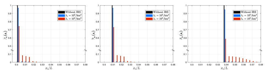
Figure 3: Probability distributions of HO trigger locations and HO execution locations, where $D=10\rm{m}$: (a) Probability distribution of HO trigger locations; (b) Probability distribution of HO execution locations ($T_{t}=120\rm{ms}$); (c) Probability distribution of HO execution locations ($T_{t}=480\rm{ms}$).

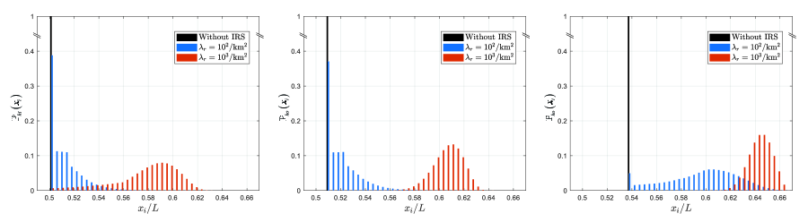
Figure 4: Probability distributions of HO trigger locations and HO execution locations, where $D=50\rm{m}$: (a) Probability distribution of HO trigger locations; (b) Probability distribution of HO execution locations ($T_{t}=120\rm{ms}$); (c) Probability distribution of HO execution locations ($T_{t}=480\rm{ms}$).

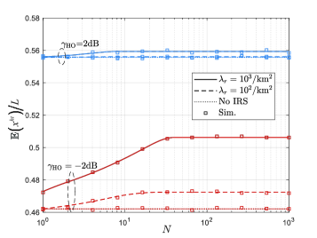
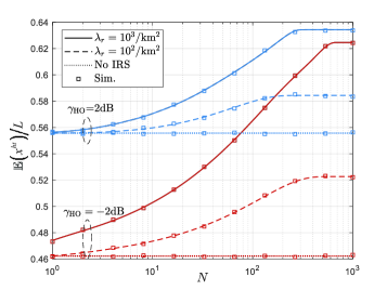
Figure 5: Ratio of the average distance from the initial location to the location where the HO is triggered to $L$ as a function of the number of IRS elements $N$ under different HO margins ${\gamma_{{\rm{HO}}}}$: (a) $D=20\rm{m}$; (b) $D=50\rm{m}$.

Figure 6: Ratio of the average distance from the initial location to the location where the HO is triggered to $L$ as a function of the IRS serving distance $D$ under different HO margins ${\gamma_{{\rm{HO}}}}$: (a) ${\gamma_{{\rm{HO}}}}=-2\rm{dB}$; (b) ${\gamma_{{\rm{HO}}}}=2\rm{dB}$.

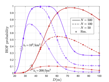
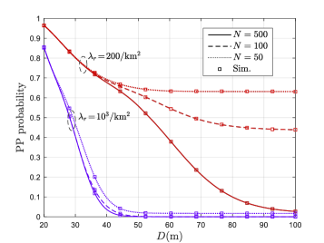
Figure 7: HOF probability and PP probability as a function of the IRS serving distance $D$ under different IRS densities $\lambda_{r}$ and numbers of IRS elements $N$: (a) HOF probability; (b) PP probability.

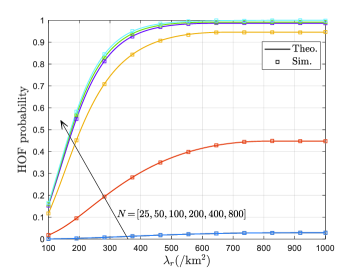
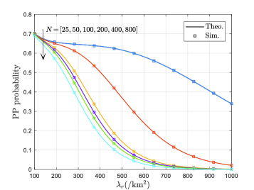
Figure 8: HOF probability and PP probability as a function of the IRS density $\lambda_{r}$ under different numbers of IRS elements $N$: (a) HOF probability; (b) PP probability.

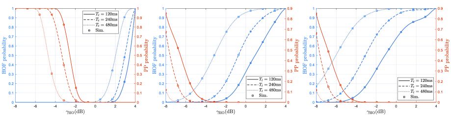
Figure 9: Relationship between the handover parameters and handover failure probability, ping-pong probability, where the blue curves represent handover failure probabilities and the red curves represent ping-pong probabilities: (a) $N$=20; (b) $N$=200; (c) $N$=500.

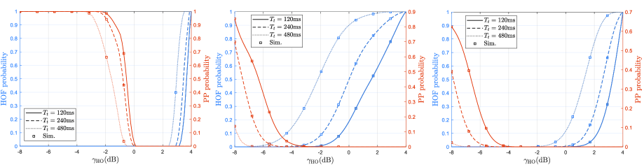
Figure 10: Relationship between the handover parameters and handover failure probability, ping-pong probability, where the blue curves represent handover failure probabilities and the red curves represent ping-pong probabilities: (a) $D$=10m; (b) $D$=50m; (c) $D$=100m.

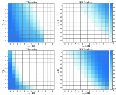
Figure 11: Heatmap of the handover failure probability and ping-pong probability under different handover parameters: (a) PP probability for $\lambda_{r}=200/\rm{km^{2}}$; (b) HOF probability for $\lambda_{r}=200/\rm{km^{2}}$; (c) PP probability for $\lambda_{r}=10^{3}/\rm{km^{2}}$; (d) HOF probability for $\lambda_{r}=10^{3}/\rm{km^{2}}$.

III-E Ping-Pong Analysis

According to (3) and (5), a PP event is assumed to occur when the user handovers back to the original BS within the threshold time $T_{p}$.

As shown in Fig. 2(d), a discrete-time model for the PP event is also proposed, in which the states after the HO is completed are modeled. The PP states are denoted as ${\mathcal{PP}}_{0}$, ${\mathcal{PP}}_{1}$, $\cdots$, ${\mathcal{PP}}_{u}$, ${\mathcal{PP}}_{t}$, and ${\mathcal{PP}}_{c}$. The states of the PP are defined as follows. ${\mathcal{PP}}_{0}$ denotes the state in which the HO is incomplete. ${\mathcal{PP}}_{1}$ indicates that the HO is complete. If the HO to the original BS is not triggered, the state transitions from ${\mathcal{PP}}_{k}$ to ${\mathcal{PP}}_{k+1}$ $\left({k\in\left\{{1,\cdots,u-1}\right\}},u\!=\!\left\lceil{\frac{{{T_{p}}-{T_{t}}}}{{{T_{d}}}}}\right\rceil\right)$. ${\mathcal{PP}}_{u}$ indicates that the PP is avoided. ${\mathcal{PP}}_{t}$ denotes that the PP condition is just satisfied, and ${\mathcal{PP}}_{c}$ denotes that PP occurs. Based on the definitions of the PP states, the corresponding state transition matrix and state vector of the discrete-time model of the PP are constructed as follows:

Lemma 8

The state transition matrix of the discrete-time model of the PP in IRS-assisted networks is given by

$$\small\begin{aligned} &{\mathcal{PP}}\!\left(i\right)=\\[-2.84526pt] &\left[{\begin{array}[]{*{20}{c}}{\!1\!-\!p_{c}^{\mathcal{H}}\!\left(i\right)}\!&\!{p_{c}^{\mathcal{H}}\!\left(i\right)}\!&0&\cdots&0&0&0\\ 0&0&\!{1\!-\!{p^{{\mathcal{P}}{\mathcal{P}}}}\!\!\left(i\right)}\!&\cdots&0&\!{{p^{{\mathcal{P}}{\mathcal{P}}}}\!\!\left(i\right)}\!&0\\ \vdots&\vdots&\vdots&\ddots&\vdots&\vdots&\vdots\\ 0&0&0&\cdots&\!\!\!{1\!\!-\!\!{p^{{\mathcal{P}}{\mathcal{P}}}}\!\!\left(i\right)}\!\!\!&\!{p^{{\mathcal{P}}{\mathcal{P}}}}\!\!\left(i\right)\!&0\\ 0&0&0&\cdots&1&0&0\\ 0&0&0&\cdots&0&0&1\\ 0&0&0&\cdots&0&0&1\end{array}}\right]\end{aligned},$$ (30)

where its size is $\left({u+3}\right)\!\times\!\left({u+3}\right)$, the element of the $n$-th row and $m$-th column represents the probability that the $n$-th state transitions to the $m$-th state, the order of states of PP is ${\mathcal{PP}}_{0}$, ${\mathcal{PP}}_{1}$, $\cdots$, ${\mathcal{PP}}_{u}$, ${\mathcal{PP}}_{t}$, ${\mathcal{PP}}_{c}$, ${p^{\mathcal{H}}_{c}}\!\left(i\right)$ indicates the probability of HO completion at the $i$-th measurement moment, and ${p^{{\mathcal{PP}}}}\!\left(i\right)$ denotes the probability of the typical user satisfying the PP condition at $i$-th measurement moment, the expressions of ${p^{\mathcal{H}}_{c}}\!\left(i\right)$ and ${p^{\mathcal{PP}}}\!\left(i\right)$ are given by

$$p_{c}^{\mathcal{H}}\left(i\right) =s_{j}^{\mathcal{H}}\left(i\right),$$ (31)

$${p^{\mathcal{PP}}}\!\!\left(i\right) =\left({s_{00}^{{{\mathcal{I}}^{t}}}\!\!\left(i\right)+s_{10}^{{{\mathcal{I}}^{t}}}\!\!\left(i\right)}\right)\times{\mathbb{P}}\left({{\rm{PP}}\left|i,{{\mathcal{I}}_{00}^{t}\vee{\mathcal{I}}_{10}^{t}}\right.}\right)$$

$$+s_{01}^{{{\mathcal{I}}^{t}}}\!\!\left(i\right){\mathbb{P}}\left({{\rm{PP}}\left|i,{{\mathcal{I}}_{01}^{t}}\right.}\right)+s_{11}^{{{\mathcal{I}}^{t}}}\!\!\left(i\right){\mathbb{P}}\left({{\rm{PP}}\left|i,{{\mathcal{I}}_{11}^{t}}\right.}\right),$$

where

$${\mathbb{P}}\left({{\rm{PP}}\left|{i,{{\mathcal{I}}^{t}_{00}}\vee{{\mathcal{I}}^{t}_{10}}}\right.}\right)=\left\{\begin{array}[]{l}1,{{{P_{o}}x_{o,i}^{-\alpha}}\mathord{\left/{\vphantom{{{P_{o}}x_{o,i}^{-\alpha}}{{P_{t}}x_{t,i}^{-\alpha}}}}\right.\kern-1.2pt}{{P_{t}}x_{t,i}^{-\alpha}}}\geq{\gamma_{\rm{HO}}}\\ 0,{{{P_{o}}x_{o,i}^{-\alpha}}\mathord{\left/{\vphantom{{{P_{o}}x_{o,i}^{-\alpha}}{{P_{t}}x_{t,i}^{-\alpha}}}}\right.\kern-1.2pt}{{P_{t}}x_{t,i}^{-\alpha}}}<{\gamma_{\rm{HO}}}\end{array}\right.,$$

$${\mathbb{P}}\left({{\rm{PP}}\left|{i,{\mathcal{I}}_{k}^{t}}\right.}\right)\!\!=\!\!\int\limits_{0}^{D}{{\mathbb{P}}\left({{\rm{PP}}\left|{i,d,{\mathcal{I}}_{k}^{t}}\right.}\right)\times f_{i}^{{\mathcal{I}}_{k}^{t}}\left(d\right){\rm{d}}d},$$

$${\mathbb{P}}\left({{\rm{PP}}\left|{i,d,{{\mathcal{I}}^{t}_{k}}}\right.}\right)\!=\!\left\{\begin{array}[]{l}1,{{{P_{o}}x_{o,i}^{-\alpha}}\mathord{\left/{\vphantom{{{P_{o}}x_{o,i}^{-\alpha}}{{\Gamma_{bf}}\left(d\right){P_{t}}x_{t,i}^{-\alpha}}}}\right.\kern-1.2pt}{{\Gamma_{bf}}\!\left(d\right){P_{t}}x_{t,i}^{-\alpha}}}\geq{\gamma_{{\rm{HO}}}}\\ 0,{{{P_{o}}x_{o,i}^{-\alpha}}\mathord{\left/{\vphantom{{{P_{o}}x_{o,i}^{-\alpha}}{{\Gamma_{bf}}\left(d\right){P_{t}}x_{t,i}^{-\alpha}}}}\right.\kern-1.2pt}{{\Gamma_{bf}}\!\left(d\right){P_{t}}x_{t,i}^{-\alpha}}}<{\gamma_{{\rm{HO}}}}\end{array}\right.\!\!\!\!,{k\in\left\{{01,\!11}\right\}}.$$ (32)

Proof:

According to the definition of the states of the PP, if the HO is executed, the state transitions from $\mathcal{PP}_{0}$ to $\mathcal{PP}_{1}$, where the probability of the HO being executed is given by Theorem 1. If the PP condition is not met, the state transitions from ${\mathcal{PP}}_{1}$ to ${\mathcal{PP}}_{2}$, $\cdots$, ${\mathcal{PP}}_{u}$, ${\mathcal{PP}}_{n}$ in turn, otherwise, the state transitions to ${\mathcal{PP}}_{t}$ and ${\mathcal{PP}}_{c}$ in turn.

The conditional probabilities of the PP are obtained from (5) and pdfs of the user-IRS distance given in Lemma 3. By integrating the conditional probabilities and state vector in Lemma 2, ${p^{\mathcal{PP}}}\!\left(i\right)$ is derived. ∎

Lemma 9

The state vector of the PP in the IRS-assisted networks at the $i$-th measurement is given by

$${{\bf{S}}^{\mathcal{PP}}}\!\!\left(i\right)={{\bf{S}}^{\mathcal{PP}}}\!\!\left(0\right){\mathcal{PP}}\!\left(0\right){\mathcal{PP}}\!\left(1\right)\cdots{\mathcal{PP}}\!\left({i-1}\right)$$ (33)

$$=\!\left[{s_{0}^{\mathcal{PP}}\!\left(i\right),s_{1}^{\mathcal{PP}}\!\left(i\right),\cdots\!,s_{u}^{\mathcal{PP}}\!\left(i\right),s_{t}^{\mathcal{PP}}\!\left(i\right),s_{c}^{\mathcal{PP}}\!\left(i\right)}\right]\!,$$

where ${{\bf{S}}^{\mathcal{PP}}}\!\!\left(0\right)=\left[{1,0,0,\cdots,0}\right]$.

Based on the discrete-time model for the PP, the expression of the PP probabilities is given by the following theorem and corollary:

Theorem 3

The PP probability of IRS-assisted networks is given by

$${\mathbb{P}}{{}_{pp}}\!=\!{\Xi_{u+3}}\!\left[{{{\bf{S}}^{{\mathcal{PP}}}}\!\!\left(0\right){{\mathcal{PP}}}\!\left(0\right){{\mathcal{PP}}}\!\left(1\right)\cdots{{\mathcal{PP}}}\!\left({I\!-\!1}\right)}\right]\!=\!s_{c}^{{\mathcal{PP}}}\!\!\left(I\right),$$ (34)

where ${\Xi_{u+3}}\left[\cdot\right]$ indicates the $(u\!+\!3)$-th element of the vector.

Corollary 3

The probability that a PP event occurs at the $i$-th measurement and the average distance from the initial location to the location where the PP event occurs are given by

$${\mathbb{P}}_{pp}\!\left({{x_{i}}}\right)={s_{t}^{{\mathcal{PP}}}\!\!\left({{x_{i}}}\right)},\ \ {\mathbb{E}}\left[{{x^{pp}}}\right]\!=\!{{\sum\limits_{i=1}^{I}{s_{t}^{{\mathcal{PP}}}\!\!\left({{x_{i}}}\right)\cdot{x_{i}}}}\mathord{\left/{\vphantom{{\sum\limits_{i=1}^{I}{s_{t}^{F}\left({{x_{i}}}\right)\cdot{x_{i}}}}{{P_{hof}}}}}\right.\kern-1.2pt}{{{\mathbb{P}}_{pp}}}}.$$ (35)

IV Numerical Results

In this section, numerical results are provided for the HO, HOF, and PP events. The results are based on the analytical derivations described in the previous sections. Monte Carlo simulations are performed to validate our analysis. The following parameters are used if not specific [22, 30, 24, 27, 33]: $\lambda_{b}=10/{\rm{km}}^{2}$, $\lambda_{r}=10^{3}/{\rm{km}}^{2}$, $P_{t}=40\rm{dBm}$, $f_{c}=3\rm{GHz}$, $\alpha=4$, $D=50\rm{m}$, $N=100$, $v=20\rm{m/s}$, $T_{d}=50\rm{ms}$, ${\gamma_{{\rm{HO}}}}=0\rm{dB}$, $T_{t}=480\rm{ms}$, $T_{p}=1\rm{s}$, $Q_{out}=-8\rm{dB}$.

IV-A Results of Handover

In this section, we focus on the effect of IRS on the HO trigger and execution locations. In particular, we quantitatively investigate the hysteresis effect of IRS-related parameters on HO using numerical results.

Figs. 3 and 4 show the probability distributions of the HO trigger and execution locations under different IRS serving distances $D$ and IRS densities $\lambda_{r}$. Compared to the network without IRS, the HO trigger locations and HO execution locations of IRS-assisted networks become irregular, as evidenced by the probabilities that triggering HO and executing HO being present at multiple locations. The HO trigger locations shift toward the target BS as the IRS density $\lambda_{r}$ and IRS serving distance $D$ increase. Specifically, the probability of HO triggering is the highest at ${{x_{i}}\mathord{\left/\right.\kern-1.2pt}L}\!=\!0.592$ when $D=50\rm{m}$, $\lambda_{r}=10^{3}/\rm{km^{2}}$, and the probability of HO triggering is higher than 90% when ${{x_{i}}\mathord{\left/\right.\kern-1.2pt}L}$ is in the interval from 0.56 to 0.62. Meanwhile, approximately 97% of the HOs are triggered at ${{x_{i}}\mathord{\left/\right.\kern-1.2pt}L}\!=\!0.503$ when $D=10\rm{m}$, $\lambda_{r}=10^{2}/\rm{km^{2}}$. For the HO execution location, increasing the TTT duration delays the HO execution, which facilitates the avoidance of PP but also presents the risk of HOF as the user needs to receive the HO command from the original BS. Specifically, the IRS further delays HO locations, e.g., a significant number of HO executions are distributed around ${{x_{i}}\mathord{\left/\right.\kern-1.2pt}L}\!=\!0.606$, although the HO has an 80% probability of triggering at ${{x_{i}}\mathord{\left/\right.\kern-1.2pt}L}\!<\!0.52$, when $D=50\rm{m}$, $\lambda_{r}=10^{2}/\rm{km^{2}}$.

Fig. 5 shows the effect of the number of IRS elements on the HO trigger location for different IRS serving distances, IRS densities, and HO margins. When ${\gamma_{{\rm{HO}}}}\!<\!1$, the HO trigger locations are shifted toward the original BS; otherwise, they are shifted toward the target BS. The IRS has a more significant effect on the HO trigger locations when ${\gamma_{{\rm{HO}}}}<1$, e.g., when $N=100$, $D=50\rm{m}$, $\lambda_{r}=10^{3}/\rm{km^{2}}$, ${\mathbb{E}{\left[{{x^{ht}}}\right]}\mathord{\left/\right.\kern-1.2pt}L}$ rises by 27.4% for the case of ${\gamma_{{\rm{HO}}}}=-2\rm{dB}$ compared to the case without IRS, while ${\mathbb{E}{\left[{{x^{ht}}}\right]}\mathord{\left/\right.\kern-1.2pt}L}$ only rises by 8.3% as ${\gamma_{{\rm{HO}}}}=2\rm{dB}$. Even when ${\gamma_{{\rm{HO}}}}=2\rm{dB}$, $\lambda_{r}=10^{2}/\rm{km^{2}}$, the HO location does not change significantly with IRS. Moreover, the HO trigger location will not continue to significantly change with increasing $N$ when $N$ reaches a certain value. This value increases as $D$ and $\lambda_{r}$ increases and $\gamma_{\rm{HO}}$ decreases, e.g., for the case of $\lambda_{r}={10^{3}}/\rm{km^{2}}$ and $\gamma_{\rm{HO}}=2\rm{dB}$, ${\mathbb{E}{\left[{{x^{ht}}}\right]}\mathord{\left/\right.\kern-1.2pt}L}$ does not change significantly with $N$ when $N$ reaches 7 and 300 for $D=20\rm{m}$ and $D=50\rm{m}$, respectively.

Fig. 6 shows the impact of the IRS serving distances on the HO trigger location under different IRS densities, numbers of IRS elements, and HO margins. Different IRS densities do not result in different HO trigger locations when $D$ is low. A sufficient value of $D$ is required to bring about differences between different IRS densities, whereas the effect of $N$ is not limited by $D$. For the case of ${\gamma_{{\rm{HO}}}}\!=\!2\rm{dB}$, IRS only affects the HO trigger location when $D$ is greater than 15m. Similar to the trend of the HO trigger locations with $N$, the delay in HO triggering slows down when $D$ increases. The change in the HO trigger location requires extra attention in the parameter intervals where it varies sharply.

IV-B Results of Handover Failure and Ping-Pong

In this section, we focus on analyzing the probabilities of HOF and PP in IRS-assisted networks based on the setup mentioned above. Specifically, we discuss the impact of IRS configuration parameters on HOF and PP events. We let ${\gamma_{{\rm{HO}}}}$ be $-2\rm{dB}$ to observe the trends in the PP probability.

Fig. 7 shows the probabilities of HOF and PP as functions of the IRS serving distance $D$ for different IRS densities and numbers of IRS elements. For the HOF, there exists a $D^{*}$ that makes the HOF most severe, and $D^{*}$ takes different values for different IRS element numbers and IRS densities. This is owing to the delay in the HO trigger location after the increase in $D$ (as shown in Fig. 6) and the increase in interference to the user from the target BS after TTT. However, a sufficiently large IRS serving distance ensures signal strength from the original BS and helps avoid the SIR from falling below $Q_{out}$. For the PP event, since the user can connect to the IRS in the new cell after the HO, it helps the user stay in the new cell. When the IRS density is large ($\lambda_{r}=10^{3}/\rm{km^{2}}$), the probability that a user can connect to an IRS in the new cell rises rapidly with $D$ and the user is close to the IRS. Thus, the PP probability decreases rapidly with $D$ and a large $N$ is not required to avoid PP in this case.

Fig. 8 shows the probabilities of HOF and PP as functions of IRS density for different numbers of IRS elements. There are trade-offs between HOF and PP in IRS density and IRS element number, where a higher IRS density or a larger IRS element number indicates more HOFs but fewer PPs. Therefore, when the IRS density and number of IRS elements are large, HOF should be considered first; otherwise, PP should be avoided. In particular, the PP probability decreases by 48%, and the HOF probability increases by 90% when $N$ reaches 100 and $\lambda_{r}=500/\rm{km^{2}}$, but with only a 7% increase in HOF and a 7% drop in PP as $N$ continues to rise to $800$. As the IRS density increases, the trend of HOF increase slows down, yet the trend of the PP decrease remains nearly constant until its probability is less than 0.1.

IV-C Optimal Settings of TTT and HO Margin

The HO parameters (i.e., TTT and HO margin) are easier to configure than the network deployment parameters (e.g., IRS density), and changes in the HO parameters do not significantly affect the performance of other networks (e.g., spectral efficiency). Therefore, selecting the optimal HO parameters is a convenient and effective method to improve the HO performance. In this section, the optimal HO parameters in IRS-assisted networks are mined to minimize the probabilities of HOF and PP. The trends in the optimal HO parameters under different IRS configurations are also discussed.

Fig. 9 shows the trade-off between the HOF and PP when the HO parameters are set under different IRS element numbers. Greater TTT and HO margins postpone HO execution, avoiding some PPs but leading to HOFs. Thus, a relatively high TTT requires a low HO margin to balance HOF and PP. As $N$ increases, the HO locations shift toward the target BS. Therefore, the appropriate HO margin under different TTTs decreases with increasing $N$ to back off the HO locations. Moreover, the optimal HO parameters decrease as $N$ increases. In particular, with a target of less than 5% for both HOF and PP, when TTT is configured as 240ms, the ranges of suitable HO margins are $[-2.2,1.5]\rm{dB}$ and $[-6,-3]\rm{dB}$ for $N=20$ and $N=200$, respectively. However, when $N=500$, only $\gamma_{\rm{HO}}\!=\!-6.2\rm{dB}$ satisfies this requirement; other TTT configurations must be considered in this case.

Fig. 10 shows the trade-off between HOF and PP when setting the HO parameters under different IRS serving distances. Combining the conclusions of Figs. 6 and 7(a), increasing $D$ delays the HO location, but a sufficient $D$ prevents HOF. Therefore, as $D$ increases, the optimal HO margin interval first shifts to smaller values and then expands. In particular, with a target of less than 5% for both HOF and PP, when TTT is configured as 240 ms, the reasonable HO margin intervals are $[-2.4,3]\rm{dB}$, $[-6,-2.4]\rm{dB}$, and $[-6.3,1]\rm{dB}$ for cases of $D=10\rm{m}$, $D=50\rm{m}$, and $D=100\rm{m}$, respectively.

A heatmap of the HOF and PP is depicted in Fig. 11 for detailed parameter settings under different IRS densities. The trends of HOF and PP with TTT and the HO margins are opposite. As the IRS density increases, the appropriate HO margin tends to decrease. For instance, when both the HOF and PP probabilities are desired to be less than 0.1%, the broadest TTT choices occur at $\gamma\!=\!0\rm{dB}$ and $\gamma\!=\!-6\rm{dB}$ for the cases of $\lambda_{r}\!=\!200/\rm{km^{2}}$ and $\lambda_{r}\!=\!10^{3}/\rm{km^{2}}$, respectively. The corresponding parameters are $\left\{{{T_{t}}=100{\rm{ms}},{\gamma_{{\rm{HO}}}}=0{\rm{dB}}}\right\}$ and $\left\{{{T_{t}}=200{\rm{ms}},{\gamma_{{\rm{HO}}}}=0{\rm{dB}}}\right\}$ for the case of $\lambda_{r}\!=\!200/\rm{km^{2}}$, $\left\{{{T_{t}}=300{\rm{ms}},{\gamma_{{\rm{HO}}}}=-6{\rm{dB}}}\right\}$, $\left\{{{T_{t}}=400{\rm{ms}},{\gamma_{{\rm{HO}}}}=-6{\rm{dB}}}\right\}$, and $\left\{{{T_{t}}=500{\rm{ms}},{\gamma_{{\rm{HO}}}}=-6{\rm{dB}}}\right\}$ for the case of $\lambda_{r}\!=\!10^{3}/\rm{km^{2}}$.

V Conclusion

To analyze the effect of IRS on the HO process and minimize HOFs and PPs in IRS-assisted networks, the HO process in IRS-assisted networks was theoretically modeled via a discrete-time model, where the exact HO location with IRS signal enhancement was captured, and HO states under IRS channel fluctuations were explicitly tracked. The probability distributions of HO triggering and HO execution over user trajectories, and the probabilities of HOF and PP were deduced. The analytical expressions were highly accurate when compared to the simulation results. Furthermore, we provide a comprehensive study of the HO performance trend using the IRS configuration parameters and determine the optimal HO parameters (i.e., TTT and HO margin) in IRS-assisted networks. This study could be extended in several methods. For instance, optimization algorithms for HO parameters can be designed based on analysis, or more practical factors, such as blockage effects, can be introduced and analyzed.

-A Proof of Lemma 1

As shown in Fig. 12, $l$ is the straight line equidistant from the original BS and the target BS, $l$ intersects the user trajectory at point $\mathbf{x}_{\rm{mid}}$ whose distance from the user’s initial location is ${x_{{\rm{mid}}}}={{\left({{r_{o}^{2}-r_{t}^{2}}+{L^{2}}}\right)}\mathord{\left/\right.\kern-1.2pt}2L}$, the two regions divided by $l$ are denoted $\mathcal{B}^{o}$ for the part close to the original BS and $\mathcal{B}^{t}$ for the part close to the target BS, the regions centered on the user’s location at the $(i-1)$-th and $i$-th measurement moments ($\mathbf{x}_{i-1}$ and $\mathbf{x}_{i}$), with $D$ as the radius, are denoted as $\mathcal{A}_{i-1}$ and $\mathcal{A}_{i}$, respectively.

Consider the IRS connection states of the original BS (i.e., $k\!=\!o$) for example. When the user has not handed over the target BS, the user can connect to the IRS in $\mathcal{B}_{o}$. To consider the correlation of adjacent moments, we focus on the following three regions when deriving the state transition probabilities: (i) the region where the IRS may exist at the $i$-th measurement moment, which is denoted as ${{\mathcal{A}}^{\prime}_{i}}\!=\!{{\mathcal{A}}_{i}}\!\cap\!{{\mathcal{B}}^{o}}$ and (ii) the region where the IRS may exist at $(i\!-\!1)$-th measurement moment, denoted by ${{\mathcal{A}}^{\prime}_{i-1}}\!=\!{{\mathcal{A}}_{i-1}}\!\cap\!{{\mathcal{B}}^{o}}$; and (iii) the overlap between ${{\mathcal{A}}^{\prime}_{i}}$ and ${{\mathcal{A}}^{\prime}_{i-1}}$, which is denoted as ${\mathcal{A}}_{i,i-1}^{\cap}\!=\!{{\mathcal{A}}^{\prime}_{i-1}}\!\cap\!{{\mathcal{A}}^{\prime}_{i}}$. Thus, we obtain

$$p_{00,00}^{{{\mathcal{I}}^{s}}}\left(i\right)=p_{10,00}^{{{\mathcal{I}}^{s}}}\left(i\right)$$ (36)

$$={\mathbb{P}}\left({N\left|{{{{\mathcal{A}}^{\prime}}_{i}}}\right|=0\left|{N\left|{{{{\mathcal{A}}^{\prime}}_{i-1}}}\right|=0}\right.}\right)={\mathbb{P}}\left({N\left|{{{{\mathcal{A}}^{\prime}}_{i}}\backslash{\mathcal{A}}_{i,i-1}^{\cap}}\right|=0}\right),$$

$$p_{01,10}^{{{\mathcal{I}}^{s}}}\left(i\right)=p_{11,10}^{{{\mathcal{I}}^{s}}}\left(i\right)$$

$$={\mathbb{P}}\left({N\left|{{\mathcal{A}}_{i,i-1}^{\cap}}\right|=0\left|{N\left|{{{\mathcal{A}^{\prime}}_{i-1}}}\right|\neq 0}\right.}\right){\mathbb{P}}\left({N\left|{{{\mathcal{A}^{\prime}}_{i}}\backslash{\mathcal{A}}_{i,i-1}^{\cap}}\right|=0}\right)$$

$$=\left[{1\!-\!\frac{{{\mathbb{P}}\!\left({N\left|{{\mathcal{A}}_{i,i-1}^{\cap}}\right|\neq 0,N\left|{{{\mathcal{A}^{\prime}}_{i-1}}}\right|\neq 0}\right)}}{{{\mathbb{P}}\left({N\left|{{{\mathcal{A}^{\prime}}_{i-1}}}\right|\neq 0}\right)}}}\right]{\mathbb{P}}\!\left({N\left|{{{\mathcal{A}^{\prime}}_{i}}\backslash{\mathcal{A}}_{i,i-1}^{\cap}}\right|\!=\!0}\right)$$

$$\mathop{=}\limits^{\left(a\right)}\left[{1\!-\!\frac{{{\mathbb{P}}\left({N\left|{{\mathcal{A}}_{i,i-1}^{\cap}}\right|\neq 0}\right)}}{{{\mathbb{P}}\left({N\left|{{{\mathcal{A}^{\prime}}_{i-1}}}\right|\neq 0}\right)}}}\right]{\mathbb{P}}\left({N\left|{{{\mathcal{A}^{\prime}}_{i}}\backslash{\mathcal{A}}_{i,i-1}^{\cap}}\right|=0}\right),$$

$$p_{00,01}^{{{\mathcal{I}}^{s}}}\!\!\left(i\right)\!=\!p_{10,01}^{{{\mathcal{I}}^{s}}}\!\!\left(i\right)\!=\!1\!-\!p_{00,00}^{{{\mathcal{I}}^{s}}}\!\!\left(i\right),p_{01,10}^{{{\mathcal{I}}^{s}}}\!\!\left(i\right)\!=\!p_{11,10}^{{{\mathcal{I}}^{s}}}\!\!\left(i\right)\!=\!1\!-\!p_{01,11}^{{{\mathcal{I}}^{s}}}\!\!\left(i\right)\!,$$

where $N\left|\cdot\right|$ is the counting measure and (a) follows ${\mathcal{A}}_{i,i-1}^{\cap}\subseteq{{{\mathcal{A}}^{\prime}}_{i-1}}$. As for the state transition probabilities ${p_{ab,cd}^{{{\mathcal{I}}^{k}}}\left(i\right)},b\neq c$, since state $ab$ cannot transition to state $cd$ in one step if $b\neq c$, we have ${p_{ab,cd}^{{{\mathcal{I}}^{k}}}\left(i\right)}=0,b\neq c$. According to the null probability of a 2-D PPP, the probability that there is no IRS in region $\mathcal{A}$ is

$$\small{\mathbb{P}}\left({N\left|{\mathcal{A}}\right|=0}\right)={e^{-{\lambda_{r}}\left|{\mathcal{A}}\right|}},$$ (37)

where $\left|\cdot\right|$ is Lebesgue measure for sets. Therefore, we focus on calculating the area of regions of interest, which are given by

$$\left|{{{{\mathcal{A}}^{\prime}}_{i}}\backslash{\mathcal{A}}_{i,i-1}^{\cap}}\right|=\left\{\begin{array}[]{ll}\left|{{{\mathcal{A}}_{i}}}\right|-\left|{{{\mathcal{A}}_{i-1}}\cap{{\mathcal{A}}_{i}}}\right|,\ \ 0\leq{x_{i}}\leq{x_{{\rm{mid}}}}-\frac{D}{{\sin\theta}}\\ \left|{{{\mathcal{A}}_{i}}}\right|-\left|{{{\mathcal{A}}_{i}}\cap{{\mathcal{B}}^{t}}}\right|-\left|{{{\mathcal{A}}_{i-1}}\cap{{\mathcal{A}}_{i}}}\right|,\\ {x_{{\rm{mid}}}}-\frac{D}{{\sin\theta}}<{x_{i}}\leq{x_{{\rm{mid}}}}-\frac{D}{{\sin\theta}}+\Delta x\\ 0,\ \ {x_{{\rm{mid}}}}-\frac{D}{{\sin\theta}}+\Delta x<{x_{i}}\end{array}\right.,$$ (38)

$$\left|{{\mathcal{A}}_{i,i-1}^{\cap}}\right|=\left\{\begin{array}[]{l}\left|{{{\mathcal{A}}_{i-1}}\cap{{\mathcal{A}}_{i}}}\right|,\ \ 0\leq{x_{i}}\leq{x_{{\rm{mid}}}}-\frac{D}{{\sin\theta}}+\Delta x\\ \left|{\left({{{\mathcal{A}}_{i-1}}\cap{{\mathcal{A}}_{i}}}\right)\backslash{{\mathcal{B}}^{t}}}\right|,\\ {x_{{\rm{mid}}}}-\frac{D}{{\sin\theta}}+\Delta x<{x_{i}}\leq{x_{{\rm{mid}}}}+\frac{D}{{\sin\theta}}\\ 0,\ \ {x_{{\rm{mid}}}}+\frac{D}{{\sin\theta}}<{x_{i}}\end{array}\right.,$$

$$\left|{{{{\mathcal{A}}^{\prime}}_{i-1}}}\right|=\left\{\begin{array}[]{l}\left|{{{\mathcal{A}}_{i-1}}}\right|,\ \ 0\leq{x_{i}}\leq{x_{{\rm{mid}}}}-\frac{D}{{\sin\theta}}+\Delta x\\ \left|{{{\mathcal{A}}_{i-1}}}\right|-\left|{{{\mathcal{A}}_{i-1}}\cap{{\mathcal{B}}^{t}}}\right|,\\ {x_{{\rm{mid}}}}-\frac{D}{{\sin\theta}}+\Delta x<{x_{i}}\leq{x_{{\rm{mid}}}}+\frac{D}{{\sin\theta}}+\Delta x\\ 0,\ \ {x_{{\rm{mid}}}}+\frac{D}{{\sin\theta}}+\Delta x<{x_{i}}\end{array}\right..$$

For simplicity, $\left|{{{{\mathcal{A}}^{\prime}}_{i}}\backslash{\mathcal{A}}_{i,i-1}^{\cap}}\right|$ is approximated to 0 when $0\!\leq\!{x_{i}}\!\leq\!{x_{{\rm{mid}}}}\!-\!\frac{D}{{\sin\theta}}$. $\left|{\left({{{\mathcal{A}}_{i-1}}\!\cap\!{{\mathcal{A}}_{i}}}\right)\!\backslash{{\mathcal{B}}^{t}}}\right|$ is calculated by integration because deriving its closed-form expression is not tractable, where a polar coordinate is established with the user location at the $i$-th measurement moment as the origin and the conditions for $\left({\rho,\theta}\right)\in{\left({{{\mathcal{A}}_{i-1}}\cap{{\mathcal{A}}_{i}}}\right)\backslash{{\mathcal{B}}^{t}}}$ are: (i) $\left({\rho,\theta}\right)\in{{\mathcal{A}}_{i}}$, i.e., $0<\rho<D$, (ii) $\left({\rho,\theta}\right)\in{{\mathcal{A}}_{i-1}}$, i.e., ${0<\sqrt{\Delta{x^{2}}+{\rho^{2}}+2\rho\Delta x\cos\varphi}<D}$, (iii) $\left({\rho,\theta}\right)\in{\mathcal{B}}^{o}$, i.e., ${\left[{\rho\sin\varphi+\rho\tan\theta\cos\varphi-\tan\theta\left({{x_{{\rm{mid}}}}-{x_{i}}}\right)}\right]\left({\theta-\frac{\pi}{2}}\right)>0}$. By calculating the area of regions and substituting (37), (38) into (36), (8) is derived, where $\left|{{{\mathcal{A}}_{i-1}}\!\cap\!{{\mathcal{A}}_{i}}}\right|$, $\left|{{{\mathcal{A}}_{i-1}}\cap{{\mathcal{B}}^{t}}}\right|$, $\left|{{{\mathcal{A}}_{i}}\cap{{\mathcal{B}}^{t}}}\right|$, $\left|{\left({{{\mathcal{A}}_{i-1}}\cap{{\mathcal{A}}_{i}}}\right)\cap{{\mathcal{B}}^{o}}}\right|$ are denoted as $S_{\cap}$, ${S_{1}^{\emptyset}}$, ${S_{2}^{\emptyset}}$, and ${S^{\prime}_{\cap}}$ for the sake of simplicity.

Using the same procedures, the state transition probabilities of the IRS connection states of the target BS (i.e., $k=t$) can be obtained. Specifically, $\mathcal{A}^{\prime}_{i}$ $\mathcal{A}^{\prime}_{i-1}$ must be modified to $\mathcal{A}_{i}\cap\mathcal{B}^{t}$ and $\mathcal{A}_{i-1}\cap\mathcal{B}^{t}$, when analyzing the IRS connection state of the target BS.

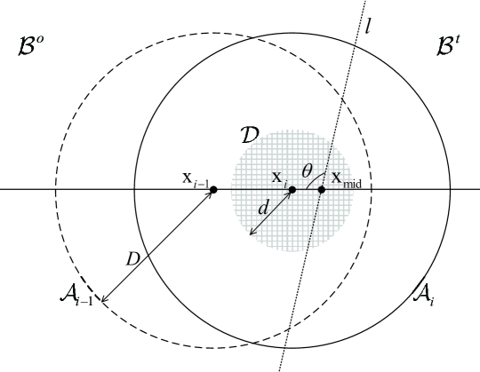
Figure 12: Regions of interest in Proof of Lemma 1 and Proof of Lemma 3, where the dashed circle is the region $\mathcal{A}_{i-1}$, the solid circle is the region $\mathcal{A}_{i}$ and the shaded circle is the region $\mathcal{D}$.

-B Proof of Lemma 3

In this proof, the regions and corresponding symbols defined in lemma 1 are used. The distance between the user and the serving IRS is denoted by $d_{0}$. As shown in Fig. 12, the region centered on the user’s location at the $i$-th measurement, where $d$ is the radius, is denoted as $\mathcal{D}$. As for the state ${{\mathcal{I}}_{01}^{o}}$, the possible locations of the IRS to which the user is connected are ${{{{\mathcal{A}}^{\prime}}_{i}}\backslash{\mathcal{A}}_{i,i-1}^{\cap}}$. Therefore, the cumulative distribution function (cdf) of $d_{0}$ under ${{\mathcal{I}}_{01}^{o}}$ is given by

$$F_{{i}}^{{\cal I}_{01}^{o}}\!\left(d\right)\!=\!{\mathbb{P}}\left({{d_{0}}<d\left|i,{{\cal I}_{01}^{o}}\right.}\right)=\!\frac{{{\mathbb{P}}\left({N\left|{{\cal D}\cap\left({{{\cal A}^{\prime}}_{i}\backslash{\cal A}_{i,i-1}^{\cap}}\right)}\right|\!\neq\!0}\right)}}{{{\mathbb{P}}\left({N\left|{{{\cal A}^{\prime}}_{i}\backslash{\cal A}_{i,i-1}^{\cap}}\right|\!\neq\!0}\right)}},$$ (39)

where ${\left|{{{\cal A}^{\prime}}_{i}\backslash{\cal A}_{i,i-1}^{\cap}}\right|}$ is given in (38) and ${\left|{{\cal D}\cap\left({{{\cal A}^{\prime}}_{i}\backslash{\cal A}_{i,i-1}^{\cap}}\right)}\right|}$ is given by

$$\left|{{\cal D}\cap\left({{\cal A^{\prime}}_{i}\backslash{\cal A}_{i,i-1}^{\cap}}\right)}\right|=$$ (40)

$$\left\{\begin{array}[]{l}\!\!\!\left|{\cal D}\right|-\left|{{\cal D}\cap{{\cal A}_{i-1}}}\right|,D-\Delta x<d\leq D,0\leq{x_{i}}\leq{x_{{\rm{mid}}}}-\frac{D}{{\sin\theta}}\\[1.42262pt] \!\!\!\cup D\!-\!\Delta x\!<\!d\!\leq\!\left({{x_{\rm{mid}}}\!-\!{x_{i}}}\right)\sin\theta,{x_{{\rm{mid}}}}\!-\!\frac{D}{{\sin\theta}}\!<\!{x_{i}}\!\leq\!{x_{{\rm{mid}}}}\!-\!\frac{D}{{\sin\theta}}\!+\!\Delta x\\ \!\!\!\left|{\cal D}\right|-\left|{{\cal D}\cap{{\cal A}_{i-1}}}\right|-\left|{{\cal D}\cap{{\cal B}^{t}}}\right|,\\ \!\!\!\left({{x_{\rm{mid}}}-{x_{i}}}\right)\sin\theta<d\leq D,{x_{{\rm{mid}}}}-\frac{D}{{\sin\theta}}<{x_{i}}\leq{x_{{\rm{mid}}}}-\frac{D}{{\sin\theta}}+\Delta x\end{array}\right.\!\!\!.$$

By calculating the area of regions and substituting (38) and (40) into (39), the cdf is derived. Thus, the corresponding pdf is $f_{{i}}^{{\mathcal{I}}_{01}^{o}}\left(d\right)={{{\rm{d}}F_{{i}}^{{\mathcal{I}}_{01}^{o}}\left(d\right)}\mathord{\left/{\vphantom{{{\rm{d}}F_{{d_{0}}}^{I_{01}^{o}}\left(d\right)}{{\rm{d}}d}}}\right.\kern-1.2pt}{{\rm{d}}d}}$, we obtain the pdf as (14).

For state ${{\mathcal{I}}_{11}^{o}}$, the possible IRS locations to which the user is connected are ${{{\mathcal{A}}^{\prime}}_{i}}$. Therefore, the cdf of $d_{0}$ under ${{\mathcal{I}}_{11}^{o}}$ is given by

$$F_{{i}}^{{\cal I}_{11}^{o}}\left(d\right)={\mathbb{P}}\left({{d_{0}}<d\left|i,{{\cal I}_{11}^{o}}\right.}\right)=\frac{{{\mathbb{P}}\left({N\left|{{\cal D}\cap{{\cal A}^{\prime}}_{i}}\right|\neq 0}\right)}}{{{\mathbb{P}}\left({N\left|{{{\cal A}^{\prime}}_{i}}\right|\neq 0}\right)}},$$ (41)

where ${\left|{{{\mathcal{A}}^{\prime}}_{i}}\right|}$ and ${\left|{{\mathcal{D}}\cap{{\mathcal{A}}^{\prime}}_{i}}\right|}$ are given by

$$\left|{{{\cal A}^{\prime}}_{i}}\right|\!=\!\left\{\begin{array}[]{ll}\left|{{{\cal A}_{i}}}\right|,\!\!\!\!\!&0\leq{x_{i}}\leq{x_{{\rm{mid}}}}-\frac{D}{{\sin\theta}}\\ \left|{{{\cal A}_{i}}}\right|\!-\!\left|{{{\cal A}_{i}}\cap{{\cal B}^{t}}}\right|,\!\!\!\!\!&{x_{{\rm{mid}}}}\!-\!\frac{D}{{\sin\theta}}<{x_{i}}\!\leq\!{x_{{\rm{mid}}}}\!+\!\frac{D}{{\sin\theta}}\end{array}\right.,$$ (42)

$$\left|{{\cal D}\cap{{\cal A}^{\prime}}_{i}}\right|=$$

$$\left\{\begin{array}[]{ll}\!\!\!\left|{\cal D}\right|,\ 0<d\leq D,{x_{i}}\leq{x_{{\rm{mid}}}}-\frac{D}{{\sin\theta}}\\ \cup 0<d\leq\left({{x_{{\rm{mid}}}}-{x_{i}}}\right)\sin\theta,{x_{{\rm{mid}}}}-\frac{D}{{\sin\theta}}<{x_{i}}\leq{x_{{\rm{mid}}}}\\ \!\!\!\left|{\cal D}\right|\!-\!\left|{{\cal D}\cap{{\cal B}^{t}}}\right|\!,\ \left({{x_{{\rm{mid}}}}\!-\!{x_{i}}}\right)\sin\theta\!\leq\!d\!\leq\!D,{x_{{\rm{mid}}}}\!-\!\frac{D}{{\sin\theta}}\!<\!{x_{i}}\!\leq\!{x_{{\rm{mid}}}}\\ \cup\left({{x_{i}}-{x_{{\rm{mid}}}}}\right)\sin\theta\leq d\leq D,{x_{{\rm{mid}}}}<{x_{i}}\leq{x_{{\rm{mid}}}}-\frac{D}{{\sin\theta}}\end{array}\right..$$

By calculating the area of regions and substituting (42) into (41), the cdf is derived. Thus the corresponding pdf is $f_{{i}}^{{\mathcal{I}}_{11}^{o}}\left(d\right)={{{\rm{d}}F_{{i}}^{{\mathcal{I}}_{11}^{o}}\left(d\right)}\mathord{\left/{\vphantom{{{\rm{d}}F_{{d_{0}}}^{I_{11}^{o}}\left(d\right)}{{\rm{d}}d}}}\right.\kern-1.2pt}{{\rm{d}}d}}$, we get the pdf as (15).

Using the same procedures as in the proofs of (14) and (15), the pdfs of the distance between the user and serving IRS under ${\mathcal{I}}_{01}^{t}$ and ${\mathcal{I}}_{11}^{t}$ can be obtained. Specifically, $\mathcal{A}^{\prime}_{i}$ and $\mathcal{A}^{\prime}_{i-1}$ need to be modified to $\mathcal{A}_{i}\cap\mathcal{B}^{t}$ and $\mathcal{A}_{i-1}\cap\mathcal{B}^{t}$ when analyzing the possible locations of the IRS to which the user is connected.

References

- [1] C. Pan et al., “Reconfigurable intelligent surfaces for 6G systems: Principles, applications, and research directions,” IEEE Commun. Mag., vol. 59, no. 6, pp. 14–20, Jun. 2021.
- [2] S. Gong et al., “Toward smart wireless communications via intelligent reflecting surfaces: A contemporary survey,” IEEE Commun. Surveys Tut., vol. 22, no. 4, pp. 2283–2314, 4th Quart., 2020.
- [3] Z. Zhang et al., “Active RIS vs. passive RIS: Which will prevail in 6G?” IEEE Trans. Commun., vol. 71, no. 3, pp. 1707–1725, Mar. 2023.
- [4] Q. Wu and R. Zhang, “Towards smart and reconfigurable environment: Intelligent reflecting surface aided wireless network,” IEEE Commun. Mag., vol. 58, no. 1, pp. 106–112, Jan. 2020.
- [5] Q. Wu, S. Zhang, B. Zheng, C. You, and R. Zhang, “Intelligent reflecting surface-aided wireless communications: A tutorial,” IEEE Trans. Commun., vol. 69, no. 5, pp. 3313–3351, May 2021.
- [6] J. Liu and H. Zhang, “Height-fixed UAV enabled energy-efficient data collection in RIS-aided wireless sensor networks,” IEEE Trans. Wireless Commun., vol. 22, no. 11, pp. 7452–7463, Nov. 2023.
- [7] J. Lyu and R. Zhang, “Hybrid active/passive wireless network aided by intelligent reflecting surface: System modeling and performance analysis,” IEEE Trans. Wireless Commun., vol. 20, no. 11, pp. 7196–7212, Nov. 2021.
- [8] M. A. Kishk and M.-S. Alouini, “Exploiting randomly located blockages for large-scale deployment of intelligent surfaces,” IEEE J. Sel. Areas Commun., vol. 39, no. 4, pp. 1043–1056, Apr. 2021.
- [9] Y. Chen et al., “Downlink performance analysis of intelligent reflecting surface-enabled networks,” IEEE Trans. Veh. Technol., vol. 72, no. 2, pp. 2082–2097, Feb. 2023.
- [10] Evolved Universal Terrestrial Radio Access (E-UTRA); Mobility Enhancements in Heterogeneous Networks, document TR 36.839, 3GPP, 2014.
- [11] H. Zhang, W. Huang, and Y. Liu, “Handover probability analysis of anchor-based multi-connectivity in 5G user-centric network,” IEEE Wireless Commun. Lett., vol. 8, no. 2, pp. 396–399, Apr. 2019.
- [12] S. Sadr and R. S. Adve, “Handoff rate and coverage analysis in multi-tier heterogeneous networks,” IEEE Trans. Wireless Commun., vol. 14, no. 5, pp. 2626–2638, May 2015.
- [13] M. Banagar, V. V. Chetlur, and H. S. Dhillon, “Handover probability in drone cellular networks,” IEEE Wireless Commun. Lett., vol. 9, no. 7, pp. 933–937, Jul. 2020.
- [14] S. Hsueh and K. Liu, “An equivalent analysis for handoff probability in heterogeneous cellular networks,” IEEE Commun. Lett., vol. 21, no. 6, pp. 1405–1408, Jun. 2017.
- [15] W. Huang, H. Zhang, and M. Zhou, “Analysis of handover probability based on equivalent model for 3D UAV networks,” in Proc. IEEE 30th Annu. Int. Symp. Pers., Indoor Mobile Radio Commun. (PIMRC), Sep. 2019, pp. 1–6.
- [16] W. Bao and B. Liang, “Stochastic geometric analysis of user mobility in heterogeneous wireless networks,” IEEE J. Sel. Areas Commun., vol. 33, no. 10, pp. 2212–2225, Oct. 2015.
- [17] R. Arshad, H. Elsawy, L. Lampe, and M. J. Hossain, “Handover rate characterization in 3D ultra-dense heterogeneous networks,” IEEE Trans. Veh. Technol., vol. 68, no. 10, pp. 10340–10345, Oct. 2019.
- [18] Technical Specification Group Radio Access Network; NR; Radio Resource Control (RRC) protocol specification, document TS 38.331, 3GPP, 2023.
- [19] M. Salehi and E. Hossain, “Stochastic geometry analysis of sojourn time in multi-tier cellular networks,” IEEE Trans. Wireless Commun., vol. 20, no. 3, pp. 1816–1830, Mar. 2021.
- [20] M. Salehi and E. Hossain, “Handover rate and sojourn time analysis in mobile drone-assisted cellular networks,” IEEE Wireless Commun. Lett., vol. 10, no. 2, pp. 392–395, Feb. 2021.
- [21] W. Huang, M. Wu, Z. Yang, K. Sun, H. Zhang, and A. Nallanathan, “Self-adapting handover parameters optimization for SDN-enabled UDN,” IEEE Trans. Wireless Commun., vol. 21, no. 8, pp. 6434–6447, Aug. 2022.
- [22] Y. He, W. Huang, H. Wei, and H. Zhang, “Effect of channel fading and time-to-trigger duration on handover performance in UAV networks,” IEEE Commun. Lett., vol. 25, no. 1, pp. 308–312, Jan. 2021.
- [23] M. Nguyen and S. Kwon, “Geometry-based analysis of optimal handover parameters for self-organizing networks,” IEEE Trans. Wireless Commun., vol. 19, no. 4, pp. 2670–2683, Apr. 2020.
- [24] X. Xu, Z. Sun, X. Dai, T. Svensson, and X. Tao, “Modeling and analyzing the cross-tier handover in heterogeneous networks,” IEEE Trans. Wireless Commun., vol. 16, no. 12, pp. 7859–7869, Dec. 2017.
- [25] H. Wei and H. Zhang, “Equivalent modeling and analysis of handover process in -tier UAV networks,” IEEE Trans. Wireless Commun., vol. 22, no. 12, pp. 9658–9671, Dec. 2023.
- [26] Y. Guo and H. Zhang, “3D boundary modeling and handover analysis of aerial users in heterogeneous networks,” IEEE Trans. Veh. Technol., vol. 72, no. 10, pp. 13523–13529, Oct. 2023.
- [27] K. Vasudeva, M. Simsek, D. López-Pérez, and İ. Güvenç, “Analysis of handover failures in heterogeneous networks with fading,” IEEE Trans. Veh. Technol., vol. 66, no. 7, pp. 6060–6074, Jul. 2017.
- [28] H. Zhang and H. Wei, “Time-varying boundary modeling and handover analysis of UAV-assisted networks with fading,” IEEE Trans. Wireless Commun., early access, Dec. 20, 2023, doi: 10.1109/TWC.2023.3342464.
- [29] L. Jiao, P. Wang, A. Alipour-Fanid, H. Zeng, and K. Zeng, “Enabling efficient blockage-aware handover in RIS-assisted mmWave cellular networks,” IEEE Trans. Wireless Commun., vol. 21, no. 4, pp. 2243–2257, Apr. 2022.
- [30] H. Wei and H. Zhang, “An equivalent model for handover probability analysis of IRS-aided networks,” IEEE Trans. Veh. Technol., vol. 72, no. 10, pp. 13770–13774, Oct. 2023.
- [31] J. Lyu and R. Zhang, “Spatial throughput characterization for intelligent reflecting surface aided multiuser system,” IEEE Wireless Commun. Lett., vol. 9, no. 6, pp. 834–838, Jun. 2020.
- [32] L. Muche, “Contact and chord length distribution functions of the Poisson-Voronoi tessellaton in high dimensions,” Adv. Appl. Probab., vol. 42, no. 1, pp. 48–68, Mar. 2010.
- [33] User Equipment (UE) Conformance Specification; Radio Transmission and Reception; Part 3: Radio Resource Management (RRM) Conformance Testing, document TS 36.521-3, 3GPP, 2023.