A unified diagrammatic approach in Liouville space to quantum transport for bosonic and fermionic reservoirs
Abstract
We present a diagrammatic approach to quantum transport based on a master equation formalism in Liouville space. It can be applied to linear and nonlinear transport in generic multi-level junctions coupled to bosonic or fermionic reservoirs and presents a convenient perturbation expansion in the strength of the coupling between the reservoirs and the junction. The Redfield theory is recovered at second order, with the partial and full secular master equations discussed. Analytical, approximate expressions are provided up to fourth order for the steady-state boson transport that generalize to multi-level systems the known formula for the low-temperature thermal conductance in the spin-boson model. The formalism is applied to the problem of heat transport in a qubit-resonator junction modeled by the quantum Rabi model. Nontrivial transport features emerge as a result of the interplay between the qubit-oscillator detuning and coupling strength. For quasi-degenerate spectra, nonvanishing steady-state coherences cause a suppression of the thermal conductance.
I Introduction
Current advances in quantum technologies allow to explore quantum effects in the transport of charge and energy in a fully controllable fashion and in the presence of several distinct transport regimes van der Wiel et al. (2000); Nazarov and Blanter (2009); Andergassen et al. (2010); Heikkilä (2013); Segal and Agarwalla (2016); Pekola and Karimi (2021). The latter are determined by the relative magnitude of few important parameters, namely the temperature, interactions or nonlinearities, and coupling between the parts of the setup that exchange particles or energy.
In a typical quantum transport setup, a number of large, noninteracting bosonic or fermionic environments, each with their own temperature and chemical potential, are connected to a common, small central system, which displays level quantization. Examples are quantum dots, low-dimensional nanostructure where a small number of electrons are confined in states according to Pauli exclusion principle, as in natural atoms Hanson et al. (2007); Laird et al. (2015), or superconducting qubits, quantum two-level systems implemented by superconducting circuits based on Josephson junctions U. Vool and M.
Devoret (2017). In these two examples of junctions, the Coulomb interaction and nonlinearity of the spectrum, respectively, can give rise to nontrivial transport features and render the transport problem generally hard to treat.
By now, several approaches have been devised, that are best suited for specific parameter regimes. For example, when the Coulomb interaction is absent or admits a perturbative treatment (e.g. mean field), the Green’s function approach provides a convenient tool for studying transport with no limitation on the coupling to the environments Bruus and Flensberg (2004); Haug and Jauho (2008, 2nd
ed); Scheer and Cuevas (2010). In the opposite regime of strongly interacting/nonlinear junctions, the kinetic equations for the reduced density operator are the tool of choice in that the junction is treated exactly and the coupling to the environments is addressed in some approximate, non-necessarily perturbative, fashion Leggett et al. (1987); J. König et al. (1996); Schoeller (2009); Donarini and Grifoni (2024).
In the kinetic equations approach, the junction is treated as an open quantum system and the relevant observables are calculated via the system reduced density matrix (RDM) Breuer and Petruccione (2002); Li et al. (2005); Leijnse and Wegewijs (2008); Timm (2008, 2011); Blum (2012); Weiss (2012, 4th ed.); Donarini and Grifoni (2024). The method exploits the noninteracting nature of the environments to trace them out exactly. This can result in a formulation in terms of Feynman-Vernon influence functional Feynman and Vernon
Jr. (1963); Magazzù et al. (2021) which is at the basis of the numerically-exact approach of hierarchical equations of motion Tanimura (2006); Jin et al. (2008); Tanimura (2020); Xu et al. (2022). The dynamics of the RDM can then be cast in the form of a generalized master equation where the result of the trace over the environments is encapsulated in a memory kernel Weiss (2012, 4th ed.); Magazzù and Grifoni (2022). A different route, based on the projection operator formalism yields the dynamical equation for the RDM in the form of the Nakajima-Zwanzig (NZ) equation Nakajima (1958); Zwanzig (1960). In this approach, the formal expression for the memory kernel is suitable for expansion in the system-environment coupling. Leading-order expansion of the NZ equation results in the weak coupling master equation of the Redfield type, suitable for further Markovian/secular approximations which, in turn, return the celebrated master equation in the Gorini-Kossakowski-Lindblad-Sudarshan form Gorini et al. (1976); Lindblad (1976), and improvements thereof Nathan and Rudner (2020); Mozgunov and Lidar (2020); McCauley et al. (2020); Trushechkin (2021); Nakamura and Ankerhold (2024).
When considering the steady state, one does not deal with time non-local expressions and a Markovian approximation is non necessary. In this case the Redfield equation, with a partial or full secular treatment, as required by consistency with perturbation theory and according to the structure of the spectrum of the junction, provides a reliable tool with the only requirement of weak coupling, in the appropriate temperature regime Kato and Tanimura (2015); Hartmann and Strunz (2020); Trushechkin (2021); Xu et al. (2021).
Higher-order phenomena involving the so-called cotunneling processes, for junctions weakly coupled to their environment, are well-studied in the context of charge transport Sukhorukov et al. (2001); Leijnse and Wegewijs (2008); Koller et al. (2010); Eckern and Wysokiński (2020); Tesser et al. (2022); Donarini and Grifoni (2024): The virtual processes involved yield a nonvanishing zero-bias conductance whereas the leading order (sequential tunneling) would predict a suppressed conductance due to Coulomb interaction in the dot (Coulomb blockade).
In the context of heat transport, a similar behavior is found at low temperatures, where the sequential tunneling current is exponentially suppressed and the dominant contribution to the heat transport of a weakly-coupled qubit junction is the cotunneling. However, results beyond the sequential tunneling in the context of bosonic heat transport are mostly limited to
qubits and are found with the generalized golden rule or the Green’s function approach Velizhanin et al. (2010); Ruokola and Ojanen (2011); Yang and Wu (2014); Yamamoto et al. (2018); Bhandari et al. (2021). A diagrammatic approach based on the Dyson series was applied to an harmonic oscillator junction in Thingna et al. (2014).
In Ferguson et al. (2021), a formalism based on the diagrammatic unravelling of the time-convolutionless master equation for a general transport setup, is carried out and compared with the results from Fermi’s golden rule. A different approach to thermal transport, based on the reaction coordinate mapping Iles-Smith et al. (2016); Strasberg et al. (2018); Anto-Sztrikacs and Segal (2021); Anto-Sztrikacs et al. (2022, 2023), can account for strong coupling to the heat or fermion baths. A review of several analytical and numerical approaches to transport in different coupling regimes is provided, e.g. in Landi et al. (2022). There, an exact expression for the heat current through a qubit coupled to two bosonic baths for , where are the slopes of the linear low-frequency Ohmic behavior of the baths’ spectral densities, has been found.
In this work, we develop a generalized master equation (ME) approach in Liouville space which allows one to treat particle and/or heat transport in generic fermionic or bosonic setups on the same footing. Specifically, we extend to the bosonic case the well known diagrammatic formulation for interacting fermionic junctions Donarini and Grifoni (2024) and apply our considerations to a concrete heat transport problem.
The starting point are the NZ equation for the RDM and the related expression for the particle/heat current. The diagrammatic formalism in Liouville space allows for a systematic perturbation expansion in the system-environment coupling using simple diagrammatic rules. Explicit expressions, up to fourth order, are given for bosonic heat transport in a generic junction.
An application to heat transport in a qubit-oscillator system, embodying the quantum Rabi model, is provided 111Part of the key results on heat transport in the Rabi model are in the companion letter.: The junction between bosonic heat baths is in this case the fundamental object of quantum electrodynamics (QED), being the archetypal system to study light matter interaction. We consider a superconducting circuit realization Blais et al. (2021) whereby a flux qubit is coupled to an LC oscillator. Superconducting circuit platform offer the possibility to operate in a vast range of coupling strengths , from weak to the ultrastrong coupling (USC) regime Yoshihara et al. (2016); Forn-Díaz et al. (2019); Kockum et al. (2019); Falci et al. (2019); Giannelli et al. (2024). In the latter case, the frequency associated to the coupling strength is of the same order of magnitude of the ones of the isolate constituents of the Rabi model and perturbative approaches in , e.g. the rotating wave approximation (RWA), which are appropriate in the quantum optical systems, break down.
We show that the heat transport properties of the setup are determined by the qubit-oscillator coupling and detuning. The coupling induces a renormalization effect on the qubit frequency that dictates the low energy spectrum of the Rabi model Hausinger and Grifoni (2010); Ashhab and Nori (2010). Application of a bias on the qubit can tune in- and out- of resonance the two elements. When the coupling is not too strong, this feature manifests itself in the so-called heat valve behavior, namely an enhancement (suppression) of the heat current when the resonance condition is (not) attained Ronzani et al. (2018); Pekola and Karimi (2021). Quasi-degeneracies in the spectrum yield steady-state coherences that suppress the thermal conductance even at high temperatures. At low temperature, when the system is essentially in its ground state and transport occurs via virtual (cotunneling) processes, quasi-degeneracies enhance multi-level interference effects that, in turn, suppress the conductance.
This work is structured as follows: In Sec. II, we introduce the transport setting described by the theory and the exact, formal results from the NZ approach to quantum transport. This is the starting point for developing, in Sec. III, the diagrammatic unravelling of the RDM and current kernels, the object that encapsulate the effect of the coupling to the environment on the system’s state and the connection between the latter and the observable of interest, the current. In Sec. VI, the results from the diagrammatic formalism are specialized to the steady-state bosonic heat transport, up to the fourth order and for a generic junction. Finally, in Sec. VII, the theory is applied to the concrete example of heat transport in the Rabi model connected to bosonic heat baths. Conclusions are left to Sec. VIII.
II Nakajima-Zwanzig approach to quantum transport
II.1 Quantum transport setup
Our starting point is the partition of the time-independent total Hamiltonian of an open quantum system linearly coupled to an environment of fermionic/bosonic baths (leads/heat baths) possibly kept at different chemical potentials and/or temperatures. The coupling term is denoted with and can be for example mediated by displacement operators or by fermionic creation/annihilation operators (tunneling Hamiltonian), according to the considered setup. The total Hamiltonian reads thus
| (1) |
where the first term describes the open system (), the portion of the total system we are interested in describing via the reduced density operator . The second term accounts for one or multiple (non-interacting) fermionic or bosonic baths (). The reservoirs are indexed by in the following so that . For a simple transport setup often one chooses for left and right, respectively. The third term is the coupling between and .
We assume it to be of the form , with and defined in the system and environment Hilbert space, respectively.
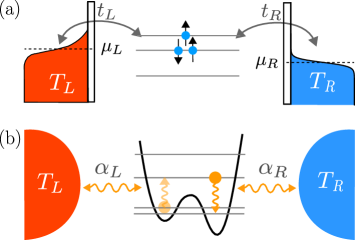
For definiteness, let us consider the two paradigmatic examples of open quantum systems, of interest in the context of transport, which are depicted in Fig. 1. The first is an interacting fermionic system, with creation/annihilation operators , tunnel-coupled to noninteracting fermionic leads with operators where . Here, is the state of where the fermion is created/annihilated and denote the momenta and spin of the electrons in the leads 222In the case where is an interacting quantum dot, ,
where is a quartic function of the fermionic operators accounting for the Coulomb interaction.. The tunneling amplitude are thus . In the second setup, an open system with energy levels is coupled to bosonic heat baths. Creation/annihilation of an excitation in the bosonic mode of bath is given by , with , . We assume the coupling to be mediated by the bath displacement operators and the system operators . The coupling strength with the th bosonic mode of bath is quantified by the frequency , see the Caldeira-Leggett model Caldeira and Leggett (1983); Weiss (2012, 4th ed.). The system Hamiltonian is left, at this stage, unspecified except that it reads in the system energy eigenbasis .
The environment and interaction terms in the general total Hamiltonian (1) are then summarized by
| (2) |
for fermions, see Fig. 1(a), and
| (3) |
for bosons, see Fig. 1(b).
Throughout the present work, we use the convention .
The environment and interaction terms can then be compactly written, for both setups, as
| (4) | ||||
where is the so-called Fock index , with the meaning and . In Eq. (4), we defined the operators and as follows. For fermions, setting , we have defined
| (5) |
For bosons, system and bath operators are defined as
| (6) |
Since the Fock and lead indices will appear together, both in the system and the bath operators, it is convenient to introduce the compact notation , namely
| (7) |
II.2 Nakajima-Zwanzig equation and current
In what follows superoperators are denoted by calligraphic letters. The time evolution of the total density matrix is given by the Liouville-Von Neumann equation
| (8) |
where . The action of the Liouvillian superoperators is given by with , or . Assume that the total density matrix at time is in the factorized initial condition , where . Here, , with , is the thermal state of the reservoir at inverse temperature and chemical potential (for bosons ). Starting from Eq. (8) and using the projection operator technique, the time evolution of the system reduced density operator can be cast as the following formally exact integro-differential equation called generalized master equation (GME)
| (9) |
of the Nakajima-Zwanzig form Nakajima (1958); Zwanzig (1960), see Appendix A for details, where the exact kernel superoperator acts on as
| (10) | ||||
Here, the projection superoperators and are defined by
| (11) |
The above formal results do not rest on being the tensor product of the reservoirs thermal states, for it suffices for to be a fixed reference state of the environment with the property .
II.2.1 Current
The general definition of current to the reservoir is given by the trace
where is the relevant current operator. Specifically, the particle and energy current operators are defined as and , respectively. For example, the fermionic particle current operator is and the corresponding charge current to reservoir reads . The associated heat current is then defined as . This coincides, at the steady state, with , for , and with , for Muralidharan and Grifoni (2012); Pekola and Karimi (2021); Tesser et al. (2022). For bosonic reservoirs, the heat current coincides with the energy current, namely , and is given by the operator . Let be the quantity to be transferred. Then a general expression for the particle/charge/heat current operator, in the fermionic or bosonic case, is
| (12) |
with for charge current in electron transport (fermion reservoirs, for the particle current) and in the case of heat current (fermion or boson reservoirs, with in the latter case). A quantity of interest in the context of heat transport is the linear thermal conductance, which gives the heat conduction properties for a small temperature bias . Setting and the temperature of the other bath , the thermal conductance is defined as the derivative of the forward current with respect to the temperature bias, in the limit of vanishing bias, namely
| (13) |
where the constraint of zero particle current is specified for the fermionic case Schulenborg et al. (2018).
Using the projection operator technique, with a similar procedure as for the GME, the current can be cast in the following form
| (14) |
(details are given in Appendix A). The current kernel has the exact expression
| (15) |
which is the same as the one for the kernel of the GME, Eq. (10), except that the last interaction Liouvillian (to the left) is here substituted by the current superoperator. The latter is simply the current operator acting from the left,
.
The steady-state RDM and current are given by the final value theorem as and , where denotes Laplace transform. Applied to the GME (9) and Eq. (14), this yields
| (16) |
Note that the steady state does not result from a Markovian approximation. It nevertheless coincides with the steady-state limit of a Markov-approximated GME, if the Markovian approximation is performed in the Schrödinger picture.
III Liouville space approach
Our aim is to systematically expand the GME in the system-environment coupling, associating diagrams to each power. This is most conveniently achieved by operating in Liouville space, where the connection between the Liouvillian superoperators and the system or environment operators is established by introducing the so-called Liouville index . The latter indicates the position of the operators with respect to the object the Liouvillian acts upon. Specifically, the action of the Liouvillian superoperators can be expressed by
where the Liouville index has the effect and . Applied to the specific systems considered here, the action of the interaction Liouville superoperator is then (, see Eq. (7))
| (17) |
Here, and are the superoperators corresponding to and , respectively. Note that the Liouville index in a superoperator does not multiply the Fock index , i.e. and . The fermionic/bosonic commutation relations translate, in Liouville space, into the commutation relations
| (18) |
Finally, the current superoperator corresponding to the current to the reservoir , Eqs. (12) and (15), in terms of Liouville indices reads
| (19) |
III.1 Trace over the environments
For a thermal reference state of the baths , the trace over the environment degree of freedom yields, using the cyclic property of the trace, the result
| (20) | ||||
Here, and are the Fermi and the Bose function of bath , respectively, according to its fermionic or bosonic statistics, with in the latter case. Contrary to the case of a superoperator, the index appearing in a function is simply the product of the two indices, e.g. .
Second order
Expansion of the exact kernel superoperators, Eqs. (10) and (15), in powers of yields the perturbation expansion of the GME and the current, see Appendix B. Since , because does not conserve the reservoirs’ particle number, the leading order is the second. It is obtained with . The Heisenberg evolution of the baths operators, for non-interacting baths, gives . Then the environment propagator results in , which yields for the RDM kernel
| (21) | ||||
Using the result (20) for the trace over the environments, we obtain
| (22) | ||||
Note that Eq. (9) with this second-order kernel (GME with Born approximation) is still nonlocal. The Markov approximation gives the Redfield I master equation, the time-local version of the GME (9) with time-dependent rates. Further, extending the upper integration limit to one obtains the Redfield II master equation with constant rates Landi et al. (2022).
Proceeding similarly for the 2nd-order current kernel, we obtain for the RDM and current kernel to leading order, in Laplace space, the following expressions
| (23) | ||||
Diagrammatically, the action of the above kernel superoperators is rendered by the single diagram
| (24) |
giving for the GME and current kernels
| (25) | ||||
where includes the constraint .
Third order
As mention above, . This entails that the third-order contribution to the kernel vanishes
| (26) | ||||
and the same holds for the current kernel. Analogously, all odd-order contributions vanish.
Fourth order
Using again , the fourth-order kernel superoperator in Laplace space reads
| (27) | ||||
where the last term, due to the action of , gives a so-called reducible contribution. A similar result is obtained for the current kernel by substituting the last tunneling Liouvillian with the current, Eq. (19). Using Eq. (18), the Wick’s theorem yields for the (non-interacting) leads’ operators Schoeller (2009); Ferguson et al. (2021)
| (28) | ||||
where . Equation (27) implies subtracting the reducible part form the correlator in Eq. (28), namely , yielding
| (29) | ||||
where , , and , with the sum extending to the number of overlapping lines between the vertices and . Indeed, diagrammatically, the action of the kernels in both the above expressions are rendered by the two irreducible diagrams, of the types and , corresponding to
| (30) |
respectively. Using Eq. (20) for the correlators, one finds for the 4th order contribution to the RDM the current kernel (the latter is obtained along similar lines) in Laplace space
| (31) | ||||
and
| (32) | ||||
Upper/lower signs refer to fermions/bosons, respectively. In analogy to Eq. (25) for the second order, the above equations are compactly written as
| (33) | ||||
where, as for the second-order diagrams, the superscript accounts for the current constraint .
III.2 Diagrammatic rules for a diagram of order
At this point, the following diagrammatic rules, valid for bosonic or fermionic systems, can be given which allow to construct the RDM and current kernels at any given order
-
•
Draw vertices connected by fermion or boson arcs. From right to left, associate to the vertices the Liouville indices and to each arc a Fock/reservoir index .
-
•
For each arc, associate to the starting (right) vertex , the vertex superoperator and the Fermi/Bose function and to the free (left) vertex the superoperator , with .
-
•
Multiply by and, for fermions, by the product for each permutation of vertices needed to bring the diagram in the fully reducible form .
-
•
To each segment connecting two consecutive vertices associate the propagator , where the sum extends to the fermion/boson arc overlapping within the segment.
-
•
For the current to reservoir : Multiply by and by the Fock index of the last fermion/boson arc and include the constraints , where is the Liouville index of the last vertex and is the reservoir index of the last fermion line.
-
•
Sum over the Liouville indices and the composite Fock/reservoir indices .
Following Magazzù and Grifoni (2022), in order to give higher-order diagrams in compact form, we introduce the boxes that account for different diagrams with swapped fermion/boson lines
| (34) | ||||
where the upper (lower) sign refers to fermion (boson) reservoirs. With this notation, the irreducible diagrams of order are compactly generated by enclosing with a fermion/boson line each of diagrams of order (reducible and irreducible) and swapping the lines via the boxes as follows
Here, we also accounted for the products of ’s required, in the fermionic case, to bring the non-crossing versions of these diagrams into the fully reducible form. Additional signs due to the crossings are contained in the boxes , see Eq. (34). To order , , , and , there correspond , , , and irreducible diagrams, respectively. For example, to 6th order there are irreducible diagrams. The unified diagrammatic Liouville-space formulation of quantum transport for fermionic and bosonic reservoirs constitutes a major result of this work.
IV Projection in the system energy eigenbasis
For practical calculations, it is useful to project the equations for the RDM and the current in the system energy eigenbasis , where . Resolving Eq. (16) in this basis via , where , we have for the NZ equation and the current in Laplace space, the formal, exact expressions
| (35) |
where correspond to the Bohr frequencies of the system, and
| (36) |
respectively. The kernel fulfills the sum rule , , dictated by probability conservation, and the property , given by the hermiticity of the RDM.
IV.1 Perturbation theory
In the system energy eignebasis, the system operators are expressed as with . From Eq. (23), this yields for the elements of the GME kernel tensor, see Eq. (35), to lowest order in ,
| (37) | ||||
Here, we have introduced, cf. Eq. (23), the function , where is the free propagator resolved in the system energy basis
| (38) |
and used . Note that, in , the subscript , () refers to the fermionic lead (bosonic bath) indexed with , see Eq. (20). In particular the (real) rates connecting the populations explicitly read
| (39) | ||||
One similarly obtains the second-order current kernel tensor elements
| (40) | ||||
With this, the current to the reservoir reads, to lowest order,
| (41) | ||||
IV.2 Partial secular 2nd-order master equation (quasi-degenerate spectrum)
The starting point is the 2nd-order steady-state Redfield ME, see Eqs. (16), (35), and (37)
| (42) |
It is worthwhile noting that the only approximation in Eq. (42) is leading order perturbation theory in the system-environment coupling: No Markovian or secular approximation have been invoked in its derivation. Assume that we can separate the transition frequencies in two classes. The first collects the Bohr frequencies much larger than the scale set by the relevant Redfield tensor elements. To the second class belong the frequencies that are of the same order of magnitude of or the ones with identical indices, i.e. .
Consistency with perturbation theory to leading order entails that Eq. (42) splits into the set of equations
| (43) | ||||
Within this partial secular approximation Cattaneo et al. (2019); Trushechkin (2021); Potts et al. (2021); Ivander et al. (2022), the surviving coherences at the steady state are those associated to the sub-spaces defined by the indices of the small transition frequencies. The remaining coherences vanish to leading order.
IV.3 Full secular master equation
For a non-degenerate spectrum with well-separated energy levels, a full secular master equation is appropriate, where populations and coherences are fully decoupled (the latter vanish at the steady state) according to
| (44) | ||||
The second of these equations gives the steady-state populations to leading order. Here, we have used the definition
| (45) |
Note that these rates are real and satisfy , which guarantees probability conservation.
V Steady-state fermionic currents
Charge transport in fermionic systems has been thoroughly investigated with diagrammatic techniques (see Donarini and Grifoni (2024) and references therein). Much less attention, however, has been devoted to bosonic heat transport in multi-level systems beyond the leading order. For this reason, in applying the general machinery developed so far, our main focus in the present work will be the bosonic heat transport.
Nevertheless, we provide here, as an illustration, some basic results of the theory specialized to fermionic transport.
From the definition of the system coupling operators in the fermionic case, Eq. (5), the second-order rates in Eq. (39) specialize to
| (46) |
where is the density of state of bath , which we assume energy-, spin-, and state-independent for simplicity and , with denoting the states of the system, see also (97).
Let us consider now a quantum dot described by the Hamiltonian coupled to fermionic leads with given by Eq. (2).
For definiteness, along the lines of one example discussed in Tesser et al. (2022), we choose
with much larger than the other setup parameters, so that the energetically unfavorable doubly-occupied configuration is essentially forbidden. For this system, the transition rates between the unoccupied state and the singly-occupied dot states read and , with . The states and cannot be connected by a rate to second order, namely , as the resulting spin-flip would require higher-order processes. The full secular treatment applied to Eq. (41) yields for the current to bath , to leading order,
| (47) |
where, from Eq. (40),
| (48) | ||||
with () for particle (energy) current. Solving the full secular master equation (44) with the symmetry and the conservation of the total probability, we obtain for the steady-state populations of the dot and . Using these results, the heat current to bath is found to be
| (49) |
where () for (). More general results for heat transport in interacting quantum dots weakly coupled fermionic baths are provided e.g. in Muralidharan and Grifoni (2012); Schulenborg et al. (2018); Tesser et al. (2022). Let us now set with and . The thermal conductance, Eq. (13), corresponding to the current formula (49) is obtained using and reads (at zero thermal bias )
| (50) |
VI Steady-state bosonic heat current
We now specialize the general formalism developed in previous sections to the problem of heat transport through a central system connected to bosonic reservoirs. The method will then be applied, in Sec. VII, to the specific model of a qubit-resonator system (Rabi model) coupled to Ohmic heat baths.
VI.1 Second-order GME and heat current
In the boson transport setting the operators are independent of the Fock index (the system coupling operators are Hermitian). We assume . Then the GME kernel, to second order, specializes to
| (51) | ||||
where, introducing the bath spectral density function , the sum over the reservoir states becomes the integral
| (52) | ||||
Here, is the correlation function of the baths operators , the time evolution being with respect to the free bath Hamiltonian. The rates are explicitly calculated in Appendix E.
The imaginary parts of the kernel matrix elements , see Eq. (LABEL:K2_bosons), can be included in the unitary part of the steady-state GME (16) as a Lamb shift term Cattaneo et al. (2019).
Similarly, according to Eq. (41), we have for the bosonic heat current to bath
| (53) |
where
| (54) | ||||
see also Ref. Thingna et al. (2012). From Eq. (53), the the zero-time correlation function enters the current expression via . This term vanishes due to the hermiticity of , and consequently does not contribute to the current.
In the full secular ME, coherences vanish to lowest order and the heat current to the bath , Eq. (53), acquires the simple form
| (55) |
Note that due to , the nonvanishing contributions are given by the rates with . According to Eqs. (LABEL:K2_bosons) and (90),
VI.2 Fourth-order heat current: Low temperature regime
At low temperature, the dominant contribution to the bosonic heat current is given by the 4th order, as the second-order current is exponentially suppressed. As shown in Appendix D, the 4th-order current kernel has the symmetry
| (56) |
which gives (assuming the coherences to vanish at the steady state),
| (57) |
Note that this same result holds for the second-order current, see Eq. (41), for vanishing coherences. The low-temperature expression for the real part of the 4th-order current kernel, in Eq. (57) is found in Appendix D to be ()
| (58) | ||||
Moreover this cotunneling current is dominant in the low temperature regime, where essentially only the ground state of the system is populated, namely , yielding for the current, Eq. (57), . Using
| (59) |
we readily find for the fourth-order contribution to the linear conductance
| (60) |
where, due to the low- cutoff imposed by at low temperature, we used . Note that the matrix elements of the coupling operators play an important role as the combination of their sign determines the overall sign of the contribution to the th-order current kernel. Equation (60) constitutes a major result of the application of the Liouville-space formalism to bosonic heat transport.
VI.3 Special case: Heat transport in a weakly-coupled qubit
In view of the application of the general results obtained in previous sections to heat transport in the quantum Rabi model, it is helpful to summarize the known results for the simpler case of a weakly-coupled spin-boson model. For the latter, expansion up to fourth order of the conductance covers the whole temperature regime Yamamoto et al. (2018). To this end, consider the case a two-level system (TLS) junction, i.e. a qubit, with energy eigenstates and of frequency . The populations of the qubit are obtained by solving the steady-state master equation in the secular approximation, Eq. (44), specialized to the TLS with rates , , where . Using Eq. (55), we obtain for the current to the reservoir Segal and Nitzan (2005a, b)
| (61) |
where () if (). Note that this expression for the heat current resembles the one obtained in the fermionic case, Eq. (49), except that here the Bose functions appear in place of the Fermi functions. To second order and for identical Ohmic baths with high-frequency cutoff, , giving , the conductance of the TLS is obtained applying Eq. (59) and reads
| (62) |
where is a dimensionless asymmetry factor. Equation (60), recovers, for the 4th-order conductance of a qubit, the known result Yamamoto et al. (2018)
| (63) |
As a concrete example, consider a qubit with Hamiltonian
coupled to Ohmic heat baths according to , see Fig. 2. Here, and are given by Eq. (3) and the qubit coupling operators are .
The qubit is the two-level system defined by the lowest energy doublet of a double-well potential. This description is appropriate for a flux qubit Rasmussen et al. (2021), see Fig. 3 below, where the energy minima correspond to the flux states induced by clockwise/anti-clockwise circulating current (circular arrows in Fig. 3(a)). These states are coupled by a tunneling amplitude , which is the qubit frequency gap for an unbiased potential.
An energy bias can be induced via an applied external magnetic flux .
We choose identical Ohmic-Drude spectral densities for the heat baths with coupling strength and cutoff frequency .
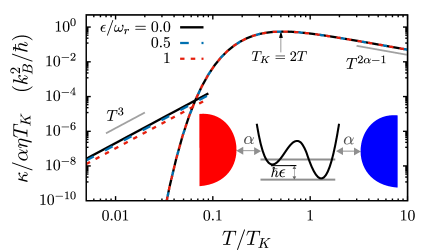
In Fig. 2 the conductance as a function of the temperature is shown for three values of the qubit bias .
It is insightful to introduce the Kondo temperature scale , defined in terms of the qubit frequency scale via . In general, this frequency scale is renormalized by the coupling to the baths Saito and Kato (2013). In our case this effect is negligible, as we assume the coupling to be weak.
The conductance displays two distinct regimes: At intermediate to high temperature, from upwards, it is dominated by , Eq. (62). With the present scaling, the curves corresponding to the different values of bias collapse. At high temperature the conductance scales as (a very good approximation of the correct nonperturbative result ). At low temperature, , the second-order conductance is exponentially suppressed, and is dominated by the fourth-order contribution , Eq. (63), which decays algebraically as .
Note that the latter does not scale with the asymmetry factor as due to the different combination of the matrix elements of the coupling operators.
As a result, the universal behavior , as shown in Fig. 2, is modulated by a bias-dependent prefactor: This is seen in the decreasing conductance for increased .
VII Application: heat transport in the quantum Rabi model
In this section we apply the machinery developed for a general transport setting in Sec. III, and specialized to the bosonic case in Sec. VI, to the concrete problem of heat transport in a qubit-oscillator system described by the quantum Rabi model, see also Magazzù et al. (2024).
VII.1 Model
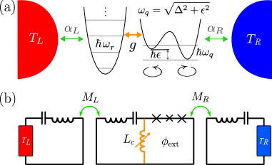
In panel (a) of Fig. 3, a schematic depiction of the heat transport setup is given, where the junction between the bosonic heat baths is formed of a qubit and an oscillator (resonator), of frequencies and , respectively, coupled with coupling strength . This system is described by the quantum Rabi model Rabi (1936, 1937). We consider a realization of the setup based on a superconducting circuit Blais et al. (2021). Figure 3(b) shows a simplified circuit model of the setup. The qubit resonator system is realized by a flux qubit (the symbol indicates a Josephson junction) sharing a common tunable inductance Forn-Díaz et al. (2010); Yoshihara et al. (2016); Magazzù et al. (2021) with a LC circuit, the oscillator. The resulting Rabi model is inductively coupled to dissipative LC circuits that realize the heat baths, the mutual inductance quantifying the coupling strength. The resonance frequencies of the baths are detuned from the low-energy spectrum of the Rabi system so that the latter sees Ohmic baths. The assumption of weak system-baths coupling is a realistic experimental regime and allows for a perturbative treatment of the system-baths interaction. The resulting Hamiltonian of the setup is given by , where the baths and interaction Hamiltonians and are given in Eq. (3) while is the system (or junction, in our quantum transport perspective) Hamiltonian and reads
| (64) |
The first and second terms describe the flux qubit (in the basis of persistent current states, see also Sec. VI.3) and the resonator, respectively, with the Pauli spin operators and and bosonic creation and annihilation operators. The third term gives the qubit-oscillator coupling. The interaction with the heat baths and is mediated by the oscillator and qubit coupling operators and , respectively. At weak coupling, the counter-rotating terms in the coupling Hamiltonian expressed in the qubit energy eigenbasis, namely and , can be safely neglected. The resulting RWA yields an easily solvable block-diagonal Hamiltonian Jaynes and Cummings (1963); Shore and Knight (1993). In the opposite regime of USC, the counter-rotating terms are non-negligible, leading to a peculiar nonperturbative effects Forn-Díaz et al. (2019); Kockum et al. (2019). This regime is described, for example, by perturbation theory on the qubit splitting , renormalized by the coupling to the oscillator Irish (2007); Ashhab and Nori (2010); Hausinger and Grifoni (2010); Zhang et al. (2013).
VII.2 Thermal conductance of the quantum Rabi model
In the following, we analyze the steady-state heat transport properties of the setup via the thermal conductance , Eq. (13), namely in the linear transport regime that characterizes the conduction in the presence of a small temperature bias. Note that the formalism developed in the previous sections has no restrictions on the temperature/chemical potential bias of the quantum transport setup and is able to describe the nonlinear transport regime at no additional cost. For the evaluations, identical Ohmic-Drude spectral densities are assumed with and . The conductance is calculated up to fourth order. The leading-order contribution is given by the full secular ME, Eqs. (55)-(13), or the partial secular ME, Eqs. (LABEL:BR_partial_secular) and (53), according to the spectral properties of the system, whereas for the fourth-order contribution we use the analytical limiting expression (60).
VII.2.1 Conductance as a function of the temperature: Universality, interference and the USC regime
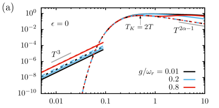
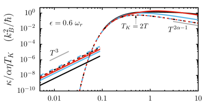
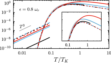
We start by considering, in Fig. 4, the temperature behavior of the conductance of the Rabi model (solid lines) up to fourth order. A comparison is made with the conductance of the TLS truncation of the Rabi model, Eqs. (62) and (63), namely the TLS formed by the ground and first excited state of the full Rabi model (dashed lines). Similarly to the case of a qubit junction, see Fig. 2, we introduce also here a Kondo-like temperature scale , defined in terms of the energy scale associated to the lowest energy doublet of the quantum Rabi model, namely . As shown below and in Magazzù et al. (2024), for the Rabi model is well described by its TLS truncation and a scaling behavior emerges in as a function of when both quantities are scaled with . Indeed is a function of , see Eq. (62).
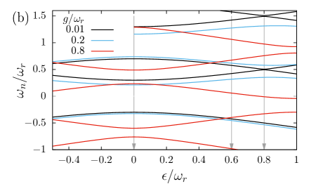
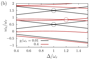
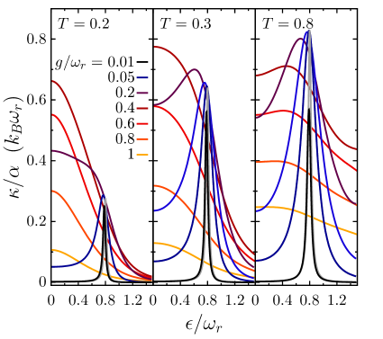
For the system is essentially in the ground state, thus , provides an excellent approximation for the 2nd-order contribution to the conductance. This expression displays however an exponential suppression at low temperature which is an artifact of lowest-order perturbation theory. Indeed, in this temperature regime, virtual processes, accounted for by the 4th-order expression for the current kernel, Eq. (58), allow for energy transfer with the system staying in its ground state Saito and Kato (2013); Yamamoto et al. (2018); Bhandari et al. (2021); Magazzù et al. (2024). This results in the algebraic low- behavior . The three panels in Fig. 4(a) show different values of the applied qubit bias for and for the same three chosen values of coupling strength , ranging from the weak to the USC regime. In particular, in moving from the first to the third panel, the qubit and oscillator frequencies approach resonance , starting from far detuned. This is reflected in Fig. 4(b) where the spectrum at weak coupling displays, at resonance, quasi-degenerate doublets of excited levels. The latter in turn result in a large coherent suppression effect of the low- conductance, with respect to the TLS counterpart. The same effect is obtained at zero bias for , see Magazzù et al. (2024). This suppression is due to inherently multi-level interference effects induced by the sum over the states in Eq. (60), which is absent in the TLS truncation, cf. Eq. (62). At resonance, USC restores the separation of the energy levels and yields an increased with approaching .
As anticipated above, in the intermediate temperature regime, where the conductance is dominated by but the temperature is low enough so that , the curves at different collapse for all values of detuning. The second-order conductance of the TLS truncation of the Rabi model has a maximum when the condition is met, as derived from Eq. (62).
Note that, in the USC regime, the scaling behavior extends to higher temperatures.
Increasing further the temperature, higher energy levels are involved and the TLS truncation breaks down: The curves depend on the details of the spectrum (and the matrix elements of the coupling operators) which are peculiar to the different values of the coupling. Deviations from the behavior , predicted for a TLS and well approximated by the limiting behavior of , are found.
It is worth noting that also the second-order conductance is suppressed, at resonance and for weak , due to steady-state coherences. Indeed, the conductance predicted by the partial secular master equation, solid, black curve for in Fig. 4(a), is smaller than the one calculated in the full secular approximation (solid gray line in the same panel, see the inset). Due to a truncation to the first five levels used in the partial secular ME, its high-temperature behavior is not reliable and thus omitted. An illustration of the emergent steady-state coherences in the presence of quasi-degenerate levels at second order is provided in Appendix F for a three-level truncation of the full Rabi model.
VII.2.2 Conductance vs. qubit-oscillator detuning: Transition from resonant to shifted, broadened peaks
Coherent effects at the level of second order are also displayed in Figs. 5 and 6, where the conductance vs. the qubit-oscillator detuning is analysed in a temperature regime where .
The transport features shown in these figures result from the interplay between the qubit-resonator coupling strength and the detuning.
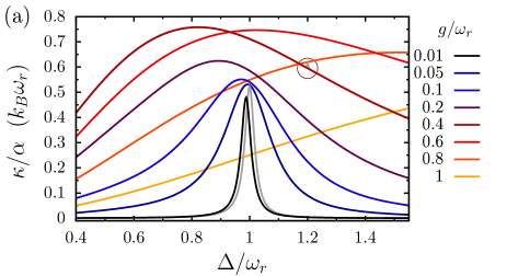
In Fig. 5(a), is plotted as a function of the qubit splitting , at zero qubit bias, for several values of the qubit-oscillator coupling strength, well into the USC regime.
At weak coupling, the conductance is sharply peaked at resonance, and suppressed elsewhere. At resonance, the weak-coupling spectrum displays quasi-degeneracies, indicated by the black circles in Fig. 5(b), that, as already seen in Fig. 4, entail a deviation of the conductance from the full secular approximation. The latter is depicted as a grey line. The result from the partial secular ME shows a suppressed peak and a Lamb shift (black line).
Increasing the coupling, the peaks broaden and move towards values of smaller than . However, in the nonperturbative coupling regime, the maxima are found at .
Intuition on these three regimes across the range of coupling considered in Fig. 5, namely resonant peak, broadened peaks for , and maxima for , is given by the approximate treatments of the quantum Rabi model summarized in Appendix G, see also Magazzù et al. (2024). At weak coupling, the RWA shows that the matrix elements of the coupling operators are suppressed everywhere except at the resonance condition, see Eq. (112). At larger , Van Vleck perturbation theory in , a second-order treatment which includes in a perturbative way the counter-rotating terms in the qubit-oscillator coupling Hamiltonian Hausinger and Grifoni (2008), predicts a shift of the resonance condition to negative detuning , as pointed out below
Eq. (109). Finally, at large coupling, in the nonperturbative regime, the generalized rotating-wave approximation Irish (2007), which is perturbative in the qubit parameter down-renormalized by the coupling to the oscillator, requires a large bare splitting, , in order to achieve the resonance condition, see Eq. (124).
For values of larger than , the results from the full secular ME essentially reproduce those of the partial secular ME, with the exception of the degeneracy at for , see the dark-red circle in Fig. 5(b). In this case, the partial secular approximation corrects an unphysical jump given by the full secular approximation, as highlighted by the dark-red circle in Fig. 5(a).
The behavior of the conductance as a function of the qubit bias with fixed displays, at low , resonant peaks when the qubit frequency matches . Upon increasing ,
undergoes a transition from resonant peaks to a broadened zero-bias maxima Magazzù et al. (2024).
This is shown in Fig. 6, where the case is considered.
Similarly to Figs. 4 and 5, at resonance and weak coupling, the spectrum presents quasi-degeneracies, see Fig. 4(b), that entail nonzero steady-state coherences. The latter result in a suppression of the conduction peak, with respect to the full secular approximation (gray curves) and a Lamb-shift to negative detuning, see also Magazzù et al. (2024).
This transition from resonant peaks to broad zero-bias maxima is reproduced at different temperatures: The suppression of the weak-coupling resonance peak is proportionally larger at higher temperature, consistently with increased steady-state coherences, see Fig. 7 in Appendix F, and the onset of the zero-bias maxima occurs at larger the larger the temperature.
These results show how the conduction properties of the quantum Rabi model, in a realistic implementation based on superconducting circuits, can be tuned by acting on the qubit parameters and on the qubit-oscillator coupling. The application showcases the nontrivial features of quantum heat transport of a system weakly coupled to heat baths which can be easily accessed with the diagrammatic technique presented in this work.
VIII Conclusions
In this work, we have developed a unified treatment of quantum transport in nanojunctions coupled to fermionic or bosonic baths. The treatment, based on a generalized master equation approach in Liouville space to open quantum systems, is suitable for a perturbation expansion in the system-baths coupling. Nevertheless, nonperurbative results are also possible with suitable diagram selections to all order Donarini and Grifoni (2024).
While the fermionic case has already being extensively investigated in the context of charge transport in quantum dot systems, bosonic heat transport beyond the leading order in multi-level systems has not yet received the same attention.
The diagrammatic method described in this work allowed us to obtain analytical, approximate expressions for the steady-state bosonic heat transport in multi-level systems up to the so-called cotunneling level, namely to fourth order in the system-baths coupling. At the level of second order, projection in the system eigenbasis reproduces the Redfield equation.
Though the method can be directly applied to the nonlinear transport regime, we focused on linear transport: Known results for the spin-boson model are reproduced, and novel results for generic multilevel systems are obtained.
The low-temperature thermal conductance is dominated by fourth-order processes where heat transfer between the baths occurs via virtual transitions in the system. For quasi-degenerate excited states, interference effects yield a large suppression of the conductance. This is an exquisite multi-level effect which is not displayed by two-level junctions (i.e. qubits). We note here that the computational cost of numerically-exact methods such as the HEOM, grows fast with the Hilbert space dimension of the system and therefore low-temperature simulations can become impractical beyond two-level systems.
Our findings are illustrated with an application to a specific instance of heat transport setup where the junction is formed of a qubit-oscillator system described by the quantum Rabi model. The features of thermal transport in this system are dictated by the qubit-oscillator detuning and coupling strength. At resonance and weak coupling, the multi-level structure of the system presents quasi-degeneracies in the excited levels that induce steady-state coherences at second order and multi-level interference effects at the level of cotunneling. This is shown by studying the conductance as a function of the temperature at different detunings and by changing the qubit splitting and bias in a temperature regime where the so-called sequential tunneling (second-order) is the dominant heat transfer mechanism. Heat transport regimes are crucially influenced by the qubit-resonator coupling strength. Indeed, coherent effects are removed at large coupling due to the pronounced repulsion of the excited levels and a behavior that converge to the one of the two-level system truncation of the Rabi model is found in the USC regime. The conductance as a function of the temperature displays in this case a scaling behavior which is highlighted by introducing the Kondo-like temperature scale corresponding to the separation internal to the lowest energy doublet.
The thermal conductance as a function of the detuning, shows a transition from a resonant peak behavior at weak coupling to a broadened, shifted peaks in the USC regime. In particular, when increasing the coupling at zero applied bias on the qubit, the resonant peak broadens and moves to negative detuning, i.e. the maxima occur at values of the qubit splitting smaller than the oscillator frequency. Upon a further increase of the coupling, in the non perturbative regime, the maxima move to positive detunings as the Rabi systems behave as an effective two-level system undergoing a strong down-renormalization of its energy. When adjusting the applied bias, the weak-coupling resonant peaks make a transition to zero-bias maxima upon increasing the coupling.
The results obtained and the specific application to the quantum Rabi model, which describes the core element of circuit QED, are of relevance given the level of experimental control and extreme parameter regime achieved in superconducting setups. These are among the leading platforms for quantum information and simulation and, more broadly, provide appealing technological applications Vepsäläinen et al. (2016); Blais et al. (2020, 2021); Pekola and Karimi (2021). Moreover, in our model, the qubit-oscillator system is placed in series between the heat baths. This constitutes an inherently asymmetric, nonlinear junction and thus satisfies the criteria for displaying heat rectification Segal and Nitzan (2005a); Senior et al. (2020).
IX Acknowledgements
The authors thank A. Donarini, G. Falci, and J. Pekola for fruitful discussions. LM and MG acknowledge financial support from BMBF (German Ministry for Education and Research), Project No. 13N15208, QuantERA SiUCs. The research is part of the Munich Quantum Valley, which is supported by the Bavarian state government with funds from the Hightech Agenda Bavaria. EP acknoweldges financial support from PNRR MUR project PE0000023-NQSTI and from COST ACTION SUPQERQUMAP, CA21144.
Appendix A Nakajima-Zwanzig formalism for quantum transport
The solution of the Liouville-von Neumann equation for the total density operator is , where , with . In Laplace space
| (65) |
Let us introduce the projection superoperators
| (66) |
These definitions imply and , . Using we can obtain the useful relation
| (67) | ||||
A.1 Nakajima-Zwanzig equation for the reduced density matrix
A.2 Current
The expectation value of an operator reads
| (71) | ||||
If does not conserve the particle number in the reservoirs, as for the current , then . Using again Eq. (67), similarly as for the Nakajima-Zwanzig equation for , we have
| (72) | ||||
In the time domain
| (73) | ||||
Appendix B Series expansion of the propagator
Let us define and . We have
Now consider
| (74) | ||||
Integrating and multiplying from the left by one obtains
| (75) |
which qualifies as the self-energy in the above Dyson equation. In Laplace space
| (76) | ||||
giving the perturbative expansion in the interaction .
Appendix C 4th-order current kernel in the energy eigenbasis
.
The - and -diagram of the current kernel, applied to , the projector in the system state , result in
In the continuum limit, the sums over and turn into integrals over and , respectively. At low , the Bose-Einstein functions are different from zero only for small arguments. Thus, the processes with give the leading contributions by approximating the central fractions of Eq. (31) as
which easily solves the integral over (neglecting the principal part). The contributions to with the constraint that the system transition frequency in the central free propagators vanish, i.e. the system is in a diagonal state between the second and third vertexes, are thus given by
| (79) | ||||
Appendix D Bosonic heat current to 4th order
In the bosonic case, the 3rd and 4th lines in Eq. (79) cancel each other as well as the 5th and 6th lines. At the steady state, , we can set and . Moreover, since both the integrals are over the positive frequencies and , this results in the constraint . Finally, for the heat current to bath , we fix the bath index of the last transition to . This yields
| (80) | ||||
where the cases in the first two lines and in the third and fourth lines cancel each other and we conveniently excluded them. Including also and swapping in the last two lines of Eq. (80),
| (81) | ||||
Use of the symmetry properties and shows directly that
| (82) |
Using this result, we have for the 4th-order current (assuming the coherences to vanish at the steady state)
| (83) | ||||
Thus, assuming , we have for
| (84) | ||||
After some algebra, using the properties of the Bose-Einstein function, which gives , where to () corresponds (), we obtain for the real part ()
| (85) | ||||
Note that if or , then the resulting expression vanishes due to the sum over , or , respectively, in the first equality.
Appendix E Evaluation of and
Specializing the general expression (40) for the 2nd-order kernel to the bosonic case, the rates are defined as
Using the definition of bath spectral density function , the sum over the reservoir states becomes the integral
| (86) | ||||
where,
is the correlation function of the baths operators , the time evolution being with respect to the free bath Hamiltonian.
The quantity which enters the expression for the 2nd-order current, Eq. (53), is analogously obtained as
| (87) | ||||
In practice, to calculate the rates (we skip here the bath index ) we start from the expression in Laplace space
| (88) | ||||
where
| (89) |
Given that the following symmetries hold .
In the Ohmic case, , with an even cutoff function, the integrand is even and we can extend the integration domain to . Using we obtain
| (90) | ||||
E.1 Analytical evaluation for Ohmic-Drude spectral density
Assuming a cutoff function such that its extension to the complex plane is holomorphic except for the poles, is given by
| (91) | ||||
where 333This can be proven by setting , where and integrating over from to 0 with , and taking the limit . is the contribution from the infinitely small detour to avoid the singularity in the integration path. We can also chose to include the pole at , with a counterclockwise detour below the pole. In this case we sum the residuum and subtract the detour which contributes as . Alternatively, one can keep the , perform the contour integral, and take the limit afterward, as done in Eq. (93) below. The pole expansion of the Bose-Einstein distribution reads
| (92) |
Here, are the Matsubara frequencies. For a Ohmic-Drude spectral density function
| (93) | ||||
From Eq. (90), noting that the last term cancels with , we get
| (94) | ||||
The calculation of the bath correlation function at goes similarly as above using the pole expansion of .
| (95) | ||||
Note that the the sum over the Matsubara frequencies diverges. As shown in the main text however, the terms containing the above bath correlation function in the expression for the current, Eq. (53), cancel out.
Fermions
For completeness, we show how the calculation of the rates, analogous to the one of , is carried out in the fermionic case. Setting , close to the poles , the Fermi function can be written as . Choosing for the electronic density of states in the leads (wide-band limit) and considering that along the upper semi circle for , and 0 between and , we obtain
| (96) | ||||
Following Ref. Leijnse and Wegewijs (2008), we single out the term in the sum over and add and subtract the Euler-Mascheroni constant . At this point, using the definition of digamma function , we get
| (97) |
Here, is the bandwidth of the fermionic reservoir. Note that the third term on the right-hand side is equal to . This expression diverges logarithmically with . The rates stay however finite due to an exact cancellation of the second term on the right-hand side when performing the sum over the Fock/Liouville indices Magazzù and Grifoni (2022); Donarini and Grifoni (2024).
Appendix F Steady-state coherence for a three-level truncation of the Rabi model
The starting point is the partial secular master equation (LABEL:BR_partial_secular). To obtain analytical results for the steady state RDM, we first perform a truncation of the system to a three-level system spanned by the energy eigenstates . Further we consider the weak qubit-oscillator coupling case close to the resonance, namely . Proceeding along the same lines of Ref. Ivander et al. (2022), the elements 12, 11, and 22 of the partial secular master equation give
| (98) | ||||
where are the rates connecting the populations. Using the conservation of total probability, along with the property , the system can be written as
| (99) | ||||
where and . The solution for the coherence is
| (100) | ||||
while the populations are the solution of
| (101) | ||||
with .
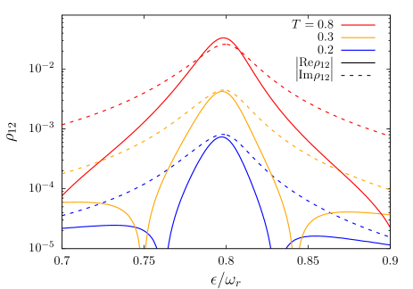
The condition of quasi-degenerate levels 1 and 2 allows for approximating . The solution for the coherence reads now
| (102) |
with , , and , and the solution for the populations is given by Eq. (101) with . The exact solution for the steady-state coherence at equilibrium in the present three-level system truncation of the Rabi model is shown in Fig. 7 as a function of the detuning between the qubit and the oscillator at weak internal coupling, , and at different temperatures.
Appendix G Analytical treatments of the Rabi model
G.1 Second-order Van Vleck perturbation theory (VVPT) in
Let us define the frequency and the couplings and . The latter are the longitudinal and transverse coupling, respectively, of the Rabi Hamiltonian expressed in the qubit energy basis. Within second-order VVPT in the qubit-resonator coupling Hausinger and Grifoni (2008) the eigenenergies of the Rabi model read ()
| (103) | ||||
where and . Note that this indexing provides the correct ordering of the eigenfrequencies only for small enough , . The corresponding eigenvectors are
| (104) | ||||
where the coefficients are given by
| (105) |
The explicit form of the transformed states in terms of the uncoupled energy eigenbasis is
| (106) | ||||
where are the normalization factors and where .
G.1.1 Zero bias,
At zero bias, the ground and first excited state read
| (107) | ||||
The matrix elements of the system’s coupling operators ( and , in the qubit energy basis) between the ground and first excited state read
| (108) |
The explicit expression for the coefficients is
| (109) |
where . Note that, at zero bias, these coefficients peak at the value of for which the condition is satisfied.
G.2 Rotating-wave approximation (RWA)
To first order in the coupling , the Van Vleck perturbation theory expressions for the eigensystem of the quantum Rabi model, Eqs. (103)-(107), reproduce the RWA results
| (110) | ||||
(), with the detuning defined as and . The corresponding eigenstates, in the energy basis of the uncoupled system, are
| (111) | ||||
with coefficients
| (112) |
Within the RWA, the relevant matrix elements of the system’s coupling operators ( and , in the qubit energy basis) read
| (113) | ||||
At resonance, while . If , the change of sign of the qubit matrix element yields the suppressed fourth-order conductance at weak coupling, see Fig. 4(a).
G.3 Generalized rotating-wave approximation (GRWA)
Within the GRWA Irish (2007); Zhang et al. (2013), the spectrum of the biased Rabi model is approximated by
| (114) | ||||
Here, , , and , where . Here, we have introduced the dressed qubit gap (), where and where are the generalized Laguerre polynomials defined by the recurrence relation
| (115) |
with and . The corresponding energy eigenstates are
| (116) | ||||
with the weights given by
| (117) |
The states
| (118) |
are superpositions of the displaced states , where is the qubit localized basis, i.e. , see the main text, and is the displacement operator.
The two-level system truncation of the Rabi model gives for the gap of the effective TLS
| (119) |
The relevant matrix elements are , where and (in the qubit localized basis). Using and , Eqs. (116) and (118) give
| (120) |
G.3.1 Zero bias,
The first two energy levels and the corresponding eigenstates read
| (121) | ||||
and, since ,
| (122) |
The gap of the effective qubit is
| (123) |
where we have defined and used and . The matrix elements of in the basis read
| (124) |
From Eq. (117), one can see that, due to the downward-renormalization of the qubit frequencies , the coefficients and peak at a bare value of for which the condition is satisfied. Note that the GRWA is perturbative in . However, this line of reasoning accounts qualitatively for the maxima at zero bias in the USC regime found in Fig. 5(a).
References
- van der Wiel et al. (2000) W. G. van der Wiel, S. De Franceschi, T. Fujisawa, J. M. Elzerman, S. Tarucha, and L. P. Kouwenhoven, “The Kondo Effect in the Unitary Limit,” Science 289, 2105 (2000).
- Nazarov and Blanter (2009) Y. V. Nazarov and Y. M. Blanter, Quantum Transport: Introduction to Nanoscience (Cambridge University Press, 2009).
- Andergassen et al. (2010) S. Andergassen, V. Meden, H. Schoeller, J. Splettstoesser, and M. R. Wegewijs, “Charge transport through single molecules, quantum dots and quantum wires,” Nanotechnology 21, 272001 (2010).
- Heikkilä (2013) T. T. Heikkilä, The Physics of Nanoelectronics: Transport and Fluctuation Phenomena at Low Temperatures (Oxford University Press, 2013).
- Segal and Agarwalla (2016) D. Segal and B. K. Agarwalla, “Vibrational heat transport in molecular junctions,” Annu. Rev. Phys. Chem. 67, 185–209 (2016).
- Pekola and Karimi (2021) J. P. Pekola and B. Karimi, “Colloquium: Quantum heat transport in condensed matter systems,” Rev. Mod. Phys. 93, 041001 (2021).
- Hanson et al. (2007) R. Hanson, L. P. Kouwenhoven, J. R. Petta, S. Tarucha, and L. M. K. Vandersypen, “Spins in few-electron quantum dots,” Rev. Mod. Phys. 79, 1217–1265 (2007).
- Laird et al. (2015) E. A. Laird, F. Kuemmeth, G. A. Steele, K. Grove-Rasmussen, J. Nygård, K. Flensberg, and L. P. Kouwenhoven, “Quantum transport in carbon nanotubes,” Rev. Mod. Phys. 87, 703–764 (2015).
- U. Vool and M. Devoret (2017) U. Vool and M. Devoret, “Introduction to quantum electromagnetic circuits,” Int. J. Circ. Theor. Appl. 45, 897–934 (2017).
- Bruus and Flensberg (2004) H. Bruus and K. Flensberg, Many-Body Quantum Theory in Condensed Matter Physics: An Introduction (OUP Oxford, 2004).
- Haug and Jauho (2008, 2nd ed) H. Haug and A.-P. Jauho, Quantum kinetics in transport and optics of semiconductors (Springer Berlin, Heidelberg, 2008, 2nd ed).
- Scheer and Cuevas (2010) E. Scheer and J. C. Cuevas, Molecular Electronics: An Introduction to Theory and Experiment (World Scientific, Singapore, 2010).
- Leggett et al. (1987) A. J. Leggett, S. Chakravarty, A. T. Dorsey, M. P. A. Fisher, A. Garg, and W. Zwerger, “Dynamics of the dissipative two-state system,” Rev. Mod. Phys. 59, 1–85 (1987).
- J. König et al. (1996) J. König, J. Schmid, H. Schoeller, and G. Schön, “Resonant tunneling through ultrasmall quantum dots: Zero-bias anomalies, magnetic-field dependence, and boson-assisted transport,” Phys. Rev. B 54, 16820–16837 (1996).
- Schoeller (2009) H. Schoeller, “A perturbative nonequilibrium renormalization group method for dissipative quantum mechanics,” Eur. Phys. J. Spec. Top. 168, 179–266 (2009).
- Donarini and Grifoni (2024) A. Donarini and M. Grifoni, Quantum Transport in Interacting Nanojunctions: A Density Matrix Approach (Springer, Berlin, 2024).
- Breuer and Petruccione (2002) H. P. Breuer and F. Petruccione, The Theory of Open Quantum Systems (Oxford University Press, Oxford, 2002).
- Li et al. (2005) Xin-Qi Li, JunYan Luo, Yong-Gang Yang, Ping Cui, and YiJing Yan, “Quantum master-equation approach to quantum transport through mesoscopic systems,” Phys. Rev. B 71, 205304 (2005).
- Leijnse and Wegewijs (2008) M. Leijnse and M. R. Wegewijs, “Kinetic equations for transport through single-molecule transistors,” Phys. Rev. B 78, 235424 (2008).
- Timm (2008) C. Timm, “Tunneling through molecules and quantum dots: Master-equation approaches,” Phys. Rev. B 77, 195416 (2008).
- Timm (2011) C. Timm, “Time-convolutionless master equation for quantum dots: Perturbative expansion to arbitrary order,” Phys. Rev. B 83, 115416 (2011).
- Blum (2012) K. Blum, Density Matrix Theory and Applications, Vol. 64 (Springer, Berlin, 2012).
- Weiss (2012, 4th ed.) U. Weiss, Quantum Dissipative Systems (World Scientific, Singapore, 2012, 4th ed.).
- Feynman and Vernon Jr. (1963) R. P Feynman and F. L. Vernon Jr., “The theory of a general quantum system interacting with a linear dissipative system,” Ann. Phys. (N.Y.) 24, 118–173 (1963).
- Magazzù et al. (2021) L. Magazzù, P. Forn-Díaz, and M. Grifoni, “Transmission spectra of the driven, dissipative Rabi model in the ultrastrong-coupling regime,” Phys. Rev. A 104, 053711 (2021).
- Tanimura (2006) Y. Tanimura, “Stochastic Liouville, Langevin, Fokker-Planck, and Master Equation Approaches to Quantum Dissipative Systems,” J. Phys. Soc. Jpn. 75, 082001 (2006).
- Jin et al. (2008) Jinshuang Jin, Xiao Zheng, and YiJing Yan, “Exact dynamics of dissipative electronic systems and quantum transport: Hierarchical equations of motion approach,” J. Chem. Phys. 128, 234703 (2008).
- Tanimura (2020) Y. Tanimura, “Numerically “exact” approach to open quantum dynamics: The hierarchical equations of motion (HEOM),” J. Chem. Phys. 153, 020901 (2020).
- Xu et al. (2022) Meng Xu, Yaming Yan, Qiang Shi, J. Ankerhold, and J. T. Stockburger, “Taming Quantum Noise for Efficient Low Temperature Simulations of Open Quantum Systems,” Phys. Rev. Lett. 129, 230601 (2022).
- Magazzù and Grifoni (2022) L. Magazzù and M. Grifoni, “Feynman-Vernon influence functional approach to quantum transport in interacting nanojunctions: An analytical hierarchical study,” Phys. Rev. B 105, 125417 (2022).
- Nakajima (1958) S. Nakajima, “On quantum theory of transport phenomena - steady diffusion,” Prog. Theor. Phys. 20, 948–959 (1958).
- Zwanzig (1960) R. Zwanzig, “Ensemble method in the theory of irreversibility,” J. Chem. Phys. 33, 1338–1341 (1960).
- Gorini et al. (1976) V. Gorini, A. Kossakowski, and E. C. G. Sudarshan, “Completely positive dynamical semigroups of N‐level systems,” J. Math. Phys. 17, 821–825 (1976).
- Lindblad (1976) G. Lindblad, “On the generators of quantum dynamical semigroups,” Comm. Math. Phys. 48, 119–130 (1976).
- Nathan and Rudner (2020) F. Nathan and M. S. Rudner, “Universal Lindblad equation for open quantum systems,” Phys. Rev. B 102, 115109 (2020).
- Mozgunov and Lidar (2020) E. Mozgunov and D. Lidar, “Completely positive master equation for arbitrary driving and small level spacing,” Quantum 4, 227 (2020).
- McCauley et al. (2020) G. McCauley, B. Cruikshank, D. I. Bondar, and K. Jacobs, “Accurate Lindblad-form master equation for weakly damped quantum systems across all regimes,” npj Quantum Inf. 6, 74 (2020).
- Trushechkin (2021) A. Trushechkin, “Unified Gorini-Kossakowski-Lindblad-Sudarshan quantum master equation beyond the secular approximation,” Phys. Rev. A 103, 062226 (2021).
- Nakamura and Ankerhold (2024) K. Nakamura and J. Ankerhold, “Qubit dynamics beyond Lindblad: Non-Markovianity versus rotating wave approximation,” Phys. Rev. B 109, 014315 (2024).
- Kato and Tanimura (2015) A. Kato and Y. Tanimura, “Quantum heat transport of a two-qubit system: Interplay between system-bath coherence and qubit-qubit coherence,” J. Chem. Phys. 143, 064107 (2015).
- Hartmann and Strunz (2020) R. Hartmann and W. T. Strunz, “Accuracy assessment of perturbative master equations: Embracing nonpositivity,” Phys. Rev. A 101, 012103 (2020).
- Xu et al. (2021) Meng Xu, J. T. Stockburger, and J. Ankerhold, “Heat transport through a superconducting artificial atom,” Phys. Rev. B 103, 104304 (2021).
- Sukhorukov et al. (2001) E. V. Sukhorukov, G. Burkard, and D. Loss, “Noise of a quantum dot system in the cotunneling regime,” Phys. Rev. B 63, 125315 (2001).
- Koller et al. (2010) S. Koller, M. Grifoni, M. Leijnse, and M. R. Wegewijs, “Density-operator approaches to transport through interacting quantum dots: Simplifications in fourth-order perturbation theory,” Phys. Rev. B 82, 235307 (2010).
- Eckern and Wysokiński (2020) U. Eckern and K. I. Wysokiński, “Two- and three-terminal far-from-equilibrium thermoelectric nano-devices in the Kondo regime,” New J. Phys. 22, 013045 (2020).
- Tesser et al. (2022) L. Tesser, B. Bhandari, P. A. Erdman, E. Paladino, R. Fazio, and F. Taddei, “Heat rectification through single and coupled quantum dots,” New J. Phys. 24, 035001 (2022).
- Velizhanin et al. (2010) K. A. Velizhanin, M. Thoss, and Haobin Wang, “Meir–Wingreen formula for heat transport in a spin-boson nanojunction model,” J. Chem. Phys. 133, 084503 (2010).
- Ruokola and Ojanen (2011) T. Ruokola and T. Ojanen, “Thermal conductance in a spin-boson model: Cotunneling and low-temperature properties,” Phys. Rev. B 83, 045417 (2011).
- Yang and Wu (2014) Yue Yang and Chang-Qin Wu, “Quantum heat transport in a spin-boson nanojunction: Coherent and incoherent mechanisms,” EPL 107, 30003 (2014).
- Yamamoto et al. (2018) T. Yamamoto, M. Kato, T. Kato, and K. Saito, “Heat transport via a local two-state system near thermal equilibrium,” New J. Phys. 20, 093014 (2018).
- Bhandari et al. (2021) B. Bhandari, P. A. Erdman, R. Fazio, E. Paladino, and F. Taddei, “Thermal rectification through a nonlinear quantum resonator,” Phys. Rev. B 103, 155434 (2021).
- Thingna et al. (2014) J. Thingna, Hangbo Zhou, and Jian-Sheng Wang, “Improved Dyson series expansion for steady-state quantum transport beyond the weak coupling limit: Divergences and resolution,” J. Chem. Phys. 141, 194101 (2014).
- Ferguson et al. (2021) M. S. Ferguson, O. Zilberberg, and G. Blatter, “Open quantum systems beyond fermi’s golden rule: Diagrammatic expansion of the steady-state time-convolutionless master equations,” Phys. Rev. Res. 3, 023127 (2021).
- Iles-Smith et al. (2016) J. Iles-Smith, A. G. Dijkstra, N. Lambert, and A. Nazir, “Energy transfer in structured and unstructured environments: Master equations beyond the Born-Markov approximations,” J. Chem. Phys. 144, 044110 (2016).
- Strasberg et al. (2018) P. Strasberg, G. Schaller, T. L. Schmidt, and M. Esposito, “Fermionic reaction coordinates and their application to an autonomous maxwell demon in the strong-coupling regime,” Phys. Rev. B 97, 205405 (2018).
- Anto-Sztrikacs and Segal (2021) N. Anto-Sztrikacs and D. Segal, “Strong coupling effects in quantum thermal transport with the reaction coordinate method,” New J. Phys. 23, 063036 (2021).
- Anto-Sztrikacs et al. (2022) N. Anto-Sztrikacs, F. Ivander, and D. Segal, “Quantum thermal transport beyond second order with the reaction coordinate mapping,” J. Chem. Phys. 156, 214107 (2022).
- Anto-Sztrikacs et al. (2023) N. Anto-Sztrikacs, A. Nazir, and D. Segal, “Effective-hamiltonian theory of open quantum systems at strong coupling,” PRX Quantum 4, 020307 (2023).
- Landi et al. (2022) G. T. Landi, D. Poletti, and G. Schaller, “Nonequilibrium boundary-driven quantum systems: Models, methods, and properties,” Rev. Mod. Phys. 94, 045006 (2022).
- Note (1) Part of the key results on heat transport in the Rabi model are in the companion article arXiv:2403.06909 (2024).
- Blais et al. (2021) A. Blais, A. L. Grimsmo, S. M. Girvin, and A. Wallraff, “Circuit quantum electrodynamics,” Rev. Mod. Phys. 93, 025005 (2021).
- Yoshihara et al. (2016) F. Yoshihara, T. Fuse, S. Ashhab, K. Kakuyanagi, S. Saito, and K. Semba, “Superconducting qubit-oscillator circuit beyond the ultrastrong-coupling regime,” Nat. Phys. 13, 44 (2016).
- Forn-Díaz et al. (2019) P. Forn-Díaz, L. Lamata, E. Rico, J. Kono, and E. Solano, “Ultrastrong coupling regimes of light-matter interaction,” Rev. Mod. Phys. 91, 025005 (2019).
- Kockum et al. (2019) F. A. Kockum, A. Miranowicz, S. De Liberato, S. Savasta, and F. Nori, “Ultrastrong coupling between light and matter,” Nat. Rev. Phys. 1, 19–40 (2019).
- Falci et al. (2019) G. Falci, A. Ridolfo, P. G. Di Stefano, and E. Paladino, “Ultrastrong coupling probed by Coherent Population Transfer,” Sci. Rep. 9, 9249 (2019).
- Giannelli et al. (2024) L. Giannelli, E. Paladino, M. Grajcar, G. S. Paraoanu, and G. Falci, “Detecting virtual photons in ultrastrongly coupled superconducting quantum circuits,” Phys. Rev. Res. 6, 013008 (2024).
- Hausinger and Grifoni (2010) J. Hausinger and M. Grifoni, “Qubit-oscillator system: An analytical treatment of the ultrastrong coupling regime,” Phys. Rev. A 82, 062320 (2010).
- Ashhab and Nori (2010) S. Ashhab and F. Nori, “Qubit-oscillator systems in the ultrastrong-coupling regime and their potential for preparing nonclassical states,” Phys. Rev. A 81, 042311 (2010).
- Ronzani et al. (2018) A. Ronzani, B. Karimi, J. Senior, Y.-C. Chang, J. T. Peltonen, C. Chen, and J. P. Pekola, “Tunable photonic heat transport in a quantum heat valve,” Nat. Phys. 14, 991–995 (2018).
- Note (2) In the case where is an interacting quantum dot, , where is a quartic function of the fermionic operators accounting for the Coulomb interaction.
- Caldeira and Leggett (1983) A. O Caldeira and A. J Leggett, “Quantum tunnelling in a dissipative system,” Ann. Phys. 149, 374–456 (1983).
- Muralidharan and Grifoni (2012) B. Muralidharan and M. Grifoni, “Performance analysis of an interacting quantum dot thermoelectric setup,” Phys. Rev. B 85, 155423 (2012).
- Schulenborg et al. (2018) J. Schulenborg, J. Splettstoesser, and M. R. Wegewijs, “Duality for open fermion systems: Energy-dependent weak coupling and quantum master equations,” Phys. Rev. B 98, 235405 (2018).
- Cattaneo et al. (2019) M. Cattaneo, G. L. Giorgi, S. Maniscalco, and R. Zambrini, “Local versus global master equation with common and separate baths: superiority of the global approach in partial secular approximation,” New J. Phys. 21, 113045 (2019).
- Potts et al. (2021) P. P. Potts, A. A. Sand Kalaee, and A. Wacker, “A thermodynamically consistent Markovian master equation beyond the secular approximation,” New J. Phys. 23, 123013 (2021).
- Ivander et al. (2022) F. Ivander, N. Anto-Sztrikacs, and D. Segal, “Quantum coherence-control of thermal energy transport: the V model as a case study,” New J. Phys. 24, 103010 (2022).
- Thingna et al. (2012) J. Thingna, J. L. García-Palacios, and J.-S. Wang, “Steady-state thermal transport in anharmonic systems: Application to molecular junctions,” Phys. Rev. B 85, 195452 (2012).
- Segal and Nitzan (2005a) D. Segal and A. Nitzan, “Heat rectification in molecular junctions,” J. Chem. Phys. 122, 194704 (2005a).
- Segal and Nitzan (2005b) D. Segal and A. Nitzan, “Spin-Boson thermal rectifier,” Phys. Rev. Lett. 94, 034301 (2005b).
- Rasmussen et al. (2021) S. E. Rasmussen, K. S. Christensen, S. P. Pedersen, L. B. Kristensen, T. Bækkegaard, N. J. S. Loft, and N. T. Zinner, “Superconducting Circuit Companion—an Introduction with Worked Examples,” PRX Quantum 2, 040204 (2021).
- Saito and Kato (2013) K. Saito and T. Kato, “Kondo Signature in heat transfer via a local two-state system,” Phys. Rev. Lett. 111, 214301 (2013).
- Magazzù et al. (2024) L. Magazzù, E. Paladino, and M. Grifoni, “Heat transport in the quantum Rabi model: Universality and ultrastrong coupling effects,” arXiv:2403.06909 (2024).
- Rabi (1936) I. I. Rabi, “On the process of space quantization,” Phys. Rev. 49, 324–328 (1936).
- Rabi (1937) I. I. Rabi, “Space quantization in a gyrating magnetic field,” Phys. Rev. 51, 652–654 (1937).
- Forn-Díaz et al. (2010) P. Forn-Díaz, J. Lisenfeld, D. Marcos, J. J. García-Ripoll, E. Solano, C. J. P. M. Harmans, and J. E. Mooij, “Observation of the Bloch-Siegert Shift in a Qubit-Oscillator System in the Ultrastrong Coupling Regime,” Phys. Rev. Lett. 105, 237001 (2010).
- Jaynes and Cummings (1963) E. T. Jaynes and F. W. Cummings, “Comparison of quantum and semiclassical radiation theories with application to the beam maser,” IEEE Proc 51, 89–109 (1963).
- Shore and Knight (1993) B. W. Shore and P. L. Knight, “The Jaynes-Cummings Model,” J. Mod. Opt. 40, 1195–1238 (1993).
- Irish (2007) E. K. Irish, “Generalized rotating-wave approximation for arbitrarily large coupling,” Phys. Rev. Lett. 99, 173601 (2007).
- Zhang et al. (2013) Yu-Yu Zhang, Qing-Hu Chen, and Yang Zhao, “Generalized rotating-wave approximation to biased qubit-oscillator systems,” Phys. Rev. A 87, 033827 (2013).
- Hausinger and Grifoni (2008) J. Hausinger and M. Grifoni, “Dissipative dynamics of a biased qubit coupled to a harmonic oscillator: analytical results beyond the rotating wave approximation,” New J. Phys. 10, 115015 (2008).
- Vepsäläinen et al. (2016) A. Vepsäläinen, S. Danilin, E. Paladino, G. Falci, and G. S. Paraoanu, “Quantum Control in Qutrit Systems Using Hybrid Rabi-STIRAP Pulses,” Photonics 3, 62 (2016).
- Blais et al. (2020) A. Blais, S. M. Girvin, and W. D. Oliver, “Quantum information processing and quantum optics with circuit quantum electrodynamics,” Nat. Phys. 16, 247–256 (2020).
- Senior et al. (2020) J. Senior, A. Gubaydullin, B. Karimi, J. T. Peltonen, J. Ankerhold, and J. P. Pekola, “Heat rectification via a superconducting artificial atom,” Commun. Phys. 3, 40 (2020).
- Note (3) This can be proven by setting , where and integrating over from to 0 with , and taking the limit .