Kantowski-Sachs and Bianchi III dynamics in $f\left(Q\right)$-gravity

Abstract

We explore the phase-space of homogeneous and anisotropic spacetimes within symmetric teleparallel $f(Q)$-gravity. Specifically, we consider the Kantowski-Sachs and locally rotational Bianchi III geometries to describe the physical space. By analyzing the phase-space, we reconstruct the cosmological history dictated by $f(Q)$-gravity and comment about the theory’s viability. Our findings suggest that the free parameters of the connection must be constrained to eliminate nonlinear terms in the field equations. Consequently, new stationary points emerge, rendering the theory cosmologically viable. We identify the existence of anisotropic accelerated universes, which may correspond to the pre-inflationary epoch.

day

I Introduction

Even though the flat Friedmann-Lemaître-Robertson-Walker (FLRW) $\Lambda$ Cold Dark Matter ($\Lambda$CDM) model passes most of the observational tests with flying colours, recent cosmological data suggest a tension between early and late Universe measurements of the expansion rate, i.e. the Hubble parameter. Specifically, Cosmic Microwave Background (CMB) data from Planck collaboration in their 2018 release Planck:2018vyg , propagated to today using flat $\Lambda$CDM suggest a value of the Hubble parameter at $H_{0}=67.4\pm 0.5$ km/s/Mpc. On the other hand, Cepheid variable stars are used as standard candles to measure the distances of galaxies with the distance ladder method, inferring a value of $H_{0}=74\pm 1.4$ km/s/Mpc (see SH0ES Riess:2019cxk ). The statistical significance between these two measurements is at 5$\sigma$. In addition, a nontrivial tension is related to the amplitude of density fluctuations at low redshifts when compared to the one predicted by CMB. The amplitude of these fluctuations, also known as linear matter perturbations, is often defined by the value of the linear matter overdensity field in spheres with a radius $8h^{-1}$Mpc. This value is called $\sigma_{8}$. The parameter $S_{8}$ is defined as $\sigma_{8}\left(\Omega_{m}/0.3\right)^{\alpha}$, where $\Omega_{m}$ is the fractional energy density of nonrelativistic matter and $\alpha$ is selected to minimize the correlation between $S_{8}$ and $\Omega_{m}$. Several weak lensing surveys such as DES DES:2017qwj , HSC HSC:2018mrq , and Heymans et al. Heymans:2020gsg , have measured $S_{8}$, but they have encountered different levels of disagreement with the value inferred from measurements by the Planck satellite. Cosmic shear data tend to recover slightly lower values of $S_{8}$ than the CMB. The Kilo-Degree Survey collaboration (KiDS) has reported the most significant disagreement so far with a significance of around 3$\sigma$ Heymans:2020gsg ; Hildebrandt:2020rno ; KiDS:2020suj ; KiDS:2020ghu ; Garcia-Garcia:2021unp . These are only some of the issues that the concordance cosmological model needs to address.

A possible alternative to solve these tensions is to consider extensions beyond $\Lambda$CDM; see DiValentino:2021izs for a review. However, incomprehension between the SNIa absolute magnitude and the Cepheid-based distance ladder instead of an exotic late- or early-time physics could be the reason for the tensions Efstathiou:2021ocp .

Because of the above, even though inflation is widely considered to be the most plausible explanation for the homogeneity and isotropy of the observable Universe, among others, most of the studies base their analysis on the fact that the Universe should be flat FLRW and, based on that, they study the evolution of perturbations. However, it could be the case that inflation does occur, but the Universe evolves towards homogeneity and isotropy starting from a more complicated metric. There have been attempts to consider an entirely arbitrary metric, meaning both inhomogeneous and anisotropic Goldwirth:1989pr ; however, the calculations become cumbersome. In this paper, we focus on homogeneous and anisotropic cosmology to extract analytical information. This class of geometries Misner1973 exhibits exciting cosmological features in the inflationary and post-inflationary epochs peebles1993principles . Nine spatially homogeneous, but generally anisotropic, Bianchi models exist based on the real three-dimensional Lie algebra classification. In these spacetimes, three-dimensional hypersurfaces are defined by the orbits of three isometries. An essential characteristic of the Bianchi models is that the physical variables depend only on time, which means that the field equations are a system of ordinary differential equations mx2 ; mx3 . In recent years, the class of anisotropic geometries has gained much interest because of anisotropic anomalies in the CMB and Large-Scale Structure (LSS) data. The origin of asymmetry and other measures of statistical anisotropy on the large scales of the Universe is a long-standing open question in cosmology. “Planck Legacy” temperature anisotropy data Planck:2018nkj show strong evidence of violating the Cosmological Principle in its isotropic aspect Fosalba:2020gls ; LeDelliou:2020kbm .

The family of spatially homogeneous Bianchi cosmologies includes as subclasses many important gravitational models, such as the Mixmaster Universe or the isotropic FLRW spacetimes mr ; Mis69 ; mis1 ; mx1 . As expected, the latter comes as a limit of Bianchi models where the anisotropy vanishes. Indeed, the flat, the open, and the closed FLRW geometries are related to the Bianchi I, V and IX spacetimes respectively WE . In general, the Bianchi spacetimes are defined by three scale factors mr ; however, the locally rotational spacetimes (LRS) admit an extra fourth isometry, and the LRS Bianchi line elements admit two independent scale factors. It is interesting to mention that the LRS Bianchi IX spacetime is related to the Kantowski-Sachs geometry ks1 .

Symmetric Teleparallel General Relativity (STGR) ngr2 ; lav1 is a geometric theory of gravity, equivalent to General Relativity. The theory is described by a metric tensor $g_{\mu\nu}\left(x^{\lambda}\right)$ and a symmetric flat connection $\Gamma_{\;\lambda\nu}^{\kappa}\left(x^{\lambda}\right)$, different from that of the Levi-Civita connection. It is assumed that the connection $\Gamma_{\;\lambda\nu}^{\kappa}\left(x^{\lambda}\right)$ admits the same symmetries with the metric tensor $g_{\mu\nu}\left(x^{\lambda}\right)$ and the corresponding Riemann tensor is assumed to have zero components (flat connection). Since the connection is considered to be symmetric, it means that its torsion also vanishes. The nonmetricity tensor plays an important role in symmetric teleparallel geometries, since it is the fundamental geometric object used to define the gravitational Action Integral lav1 and thus describe gravitational interactions.

To explain the observed cosmic acceleration rr1 ; Teg ; Komatsu ; suzuki11 in the context of symmetric teleparallel theory in a natural way, it has been proposed the employ of nonlinear terms of the nonmetricity scalar, $Q$, in the gravitational action, leading to the symmetric teleparallel $f\left(Q\right)$-theory lav2 ; lav3 . The same approach has been considered before in the case of $f\left(R\right)~{}$fr and $f\left(T\right)$ theories of gravity ft , where the Ricci scalar $R$ of the Levi-Civita connection and the torsion scalar $T$ of the teleparallel connection Weitzenb23 are considered to define the gravitational theory. For a comprehensive review on teleparallel theories of gravity see Bahamonde:2021gfp . The novelty of the $f\left(X\right)$-theories rev1 ; rev2 , where $X$ is a geometric scalar, is that new terms which are introduced in the modified field equations drive the dynamics to describe the expansion of the universe in a geometric way, without the addition of any exotic form of matter/energy cp1 .

Preliminary cosmological studies in $f\left(Q\right)$-theory have shown that it is a potential geometric dark energy candidate which can challenge the concordance model in cosmology ww0 ; ww8 ; ds00 . Numerous studies show that $f\left(Q\right)$-theory can reproduce various cosmological scenarios lym1 ; lym2 ; lym3 ; lym4 ; in nd1 , the authors determined the criteria for the existence of scaling cosmological solutions; the detailed phase-space analysis was presented in andyn1 and it indicates that $f\left(Q\right)$-theory can be used to describe not only late-time but also early-time acceleration phases of the Universe. Similar results are presented in dyn2 . The Hamiltonian analysis of $f(Q)$-theory was studied in hd1 ; hd2 ; hd3 , while quantum cosmology was investigated in qdim1 ; qdim2 . For extensions of $f\left(Q\right)$-theory we refer the reader to ex1 ; ex2 ; ex3 ; ex7 and other cosmological applications are discussed in ex4 ; ex5 ; ex6 and references therein. A recent review on the topic is Heisenberg:2023lru .

Because the connection in $f\left(Q\right)$-theory is flat and symmetric, it comes naturally that there exists a coordinate system where all the components of the connection can vanish; as a result, the covariant derivatives are reduced to partial derivatives. This characteristic coordinate system is known as the coincident gauge lav3 . Different connections, in general, affect the dynamics in a given $f(Q)$-theory. However, in the case where $f(Q)$ is a linear function, the connection becomes dynamically irrelevant and consequently, there are no differences produced by the choice of the latter. The resulting differences in the case of a non-linear theory can be easily observed in studies of isotropic and homogeneous cosmology Hohmann ; Heis2 ; Zhao and in static spherical symmetric spacetimes seb1 . When the coincident gauge is employed, the corresponding field equations of $f\left(Q\right)$-theory are of second order involving only the metric degrees of freedom, while, when we assume an arbitrary connection, the resulting field equations in the scalar-tensor representation are described by invoking two additional scalar fields mini1 ; lav3 . Although the coincident gauge can always be recovered for a given geometry, it cannot always be used blindly, when a specific assumption for the spacetime metric has been made. For instance, for a homogeneous and isotropic FLRW metric with non-zero spatial curvature, written in a diagonal form, and in the usual spherical coordinate system, the unique connection which can produce the field equations for a nonlinear function $f\left(Q\right)$ is defined in a purely non-coincident gauge Zhao . The same property is true for the case of anisotropic spacetimes with curvature dimks and non-flat inhomogeneous geometries seb1 . This happens because assuming a specific form for the spacetime metric already fixes partially the gauge, and this choice may be incompatible with the coordinate system where the connection components vanish.

The structure of the paper is as follows. In Section II we briefly discuss the basic properties and definitions of symmetric teleparallel general relativity and of the symmetric teleparallel $f\left(Q\right)$-theory of gravity. We discuss previous results for the spatially flat and isotropic universe in Section III. Homogeneous and isotropic locally rotational spacetimes with nonzero spatial curvature in symmetric teleparallel $f\left(Q\right)$-theory are introduced in Section IV. We give emphasis in the Kantowski-Sachs and Bianchi III geometries and we present the gravitational field equations in the case of vacuum for a nonlinear function $f\left(Q\right)$. Section V includes the main results of this analysis where we present a detailed analysis of the phase-space for the anisotropic cosmological model. From our analysis it follows that for specific values of the free parameters which define the connection the theory can provide the limit of General Relativity (GR) and there exist a plethora of asymptotic solutions which can describe anisotropic inflationary solutions. However, in the generic case of the connection these solutions are lost. Thus the cosmological viability of the theory constraints the free parameters of the connection as it follows from the analysis of the asymptotics. Finally, in Section VI we discuss our results.

II Symmetric Teleparallel Geometry and gravity

In teleparallel theories, parallelism at a distance is achieved by the vanishing of the curvature of the connection, i.e. $R^{\alpha}{}_{\mu\beta\nu}=0$, which makes the connection become integrable and thus it can be expressed as

$$\Gamma^{\alpha}{}_{\mu\nu}=(\Lambda^{-1})^{\alpha}{}_{\lambda}\partial_{\mu}\Lambda^{\lambda}{}_{\nu}\,,$$ (1)

where $\Lambda\in GL(4,\mathbf{R})$. In addition, symmetric means that the torsion of the connection vanishes, i.e. $T^{\alpha}{}_{\mu\nu}=2\Gamma^{\alpha}{}_{[\mu\nu]}=0$, in which case $\Lambda$ can be written as $\Lambda^{\alpha}{}_{\beta}=\partial_{\beta}\xi^{\alpha}$, with $\xi^{\alpha}$ being an arbitrary coordinate system. This leads to the symmetric teleparallel connection that can be expressed as

$$\Gamma^{\alpha}{}_{\mu\nu}=\frac{\partial x^{\alpha}}{\partial\xi^{\lambda}}\partial_{\mu}\partial_{\nu}\xi^{\lambda}\,.$$ (2)

Since $\xi^{\alpha}$ is arbitrary, we can always find a coordinate system in which the connection vanishes by performing a diffeomorphism; this is called the coincident gauge.

Notice that, the theory of gravity could be perfectly formulated just by the metric tensor, $g_{\mu\nu}$, with the kinetic term in the action being $\partial_{\alpha}g_{\mu\nu}$. However, this would not have the same symmetries as General Relativity (GR); it would violate diffeomorphism (Diff) invariance. In order to resolve that, we can employ the above $\xi$’s as Stückelberg fields and the Diff symmetry will be restored.

According to the above, the only non-trivial geometric object in a symmetric teleparallel geometry is the nonmetricity tensor, expressed as

$$Q_{\alpha\mu\nu}=\partial_{\alpha}g_{\mu\nu}-\Gamma^{\lambda}{}_{\alpha\mu}g_{\lambda\nu}-\Gamma^{\lambda}{}_{\alpha\nu}g_{\lambda\mu}=\partial_{\alpha}g_{\mu\nu}-2\frac{\partial x^{\sigma}}{\partial\xi^{\lambda}}\partial_{\alpha}\partial_{(\mu}\xi^{\lambda}g_{\nu)\sigma}\,.$$ (3)

This object transforms clearly covariantly and thus any theory formulated with it will be automatically Diff invariant.

II.1 Symmetric Teleparallel Equivalent of General Relativity

By defining the two independent traces $Q_{\mu}=Q_{\mu\nu}{}^{\nu}$ and $\tilde{Q}^{\nu}{}_{\mu\nu}$, the nonmetricity scalar is defined as

$$Q=Q_{\alpha\mu\nu}P^{\alpha\mu\nu}\,,$$ (4)

where

$$P^{\alpha}{}_{\mu\nu}=-\frac{1}{4}Q^{\alpha}{}_{\mu\nu}+\frac{1}{2}Q_{(\mu}{}^{\alpha}{}_{\nu)}+\frac{1}{4}g_{\mu\nu}(Q^{\alpha}-\tilde{Q}^{\alpha})-\frac{1}{4}\delta^{\alpha}{}_{(\mu}Q_{\nu)}\,,$$ (5)

with $\delta{\alpha}_{\mu}$ being the 4-dimensional Kronecker delta and the brackets denote symmetrization $2A_{(\mu\nu)}=A_{\mu\nu}+A_{\nu\mu}$.

As mentioned above, the curvature of the symmetric teleparallel connection (2) is zero. However, the curvature calculated from the Levi-Civita connection, $\accentset{\circ}{R}^{\alpha}{}_{\mu\beta\nu}$, is not. The relation between the nonmetricity scalar $Q$ and the Ricci scalar $\accentset{\circ}{R}$ is given by

$$\accentset{\circ}{R}=Q+\accentset{\circ}{\nabla}_{\alpha}(Q^{\alpha}-\tilde{Q}^{\alpha})\,.$$ (6)

By taking the functional integral of the above, the last term will act as a boundary term and thus contribute nothing at the dynamics of the theory. This means that GR and STGR are two dynamically equivalent theories since

$$\mathcal{S}_{\mathrm{GR}}=\int\mathrm{d}^{4}x\sqrt{-g}\accentset{\circ}{R}\sim\mathcal{S}_{\mathrm{STGR}}=\int\mathrm{d}^{4}x\sqrt{-g}Q\,.$$ (7)

What is more, any prediction of GR should be predicted by STGR as well and any solution in GR should have an analog solution in STGR. The only thing that changes is the geometric interpretation of gravitational interactions.

II.2 $f(Q)$-Theory

In the same spirit as with $f(\accentset{\circ}{R})$-theories, we can generalize the nonmetricity scalar (4) with a general function of it, so that the new action will read

$$\mathcal{S}_{f(Q)}=\int\mathrm{d}^{4}x\sqrt{-g}f(Q)\,.$$ (8)

Since the action contains non-linear terms in $Q$, not only the two theories are no longer equivalent, but also solutions, like the non-flat FLRW one, which worked fine in the coincident gauge STGR, are no longer solutions in $f(Q)$.

So in this case, we have both the metric and the connection (2) as fundamental variables. Varying the action (8) with respect to the metric, we get

$$\frac{2}{\sqrt{-g}}\nabla_{\lambda}(\sqrt{-g}f^{\prime}(Q)P^{\lambda}_{\;\;\mu\nu})-\frac{1}{2}f(Q)g_{\mu\nu}+f^{\prime}(Q)(P_{\mu\rho\sigma}Q_{\nu}{}^{\rho\sigma}-2Q_{\rho\sigma\mu}P^{\rho\sigma}{}_{\nu})=0\,,$$ (9)

where the prime denotes differentiation with respect to the argument, i.e. $f^{\prime}(Q)=f_{,Q}$. Respectively, varying the action with respect to the connection we get

$$\nabla_{\mu}\nabla_{\nu}(\sqrt{-g}f^{\prime}(Q)P^{\mu\nu}_{\quad\sigma})=0\,.$$ (10)

In the coincident gauge, the latter is satisfied identically.

III Flat FLRW Cosmology in $f(Q)$ gravity

Consider a homogeneous and isotropic flat FLRW metric of the form

$$\mathrm{d}s^{2}=-N(t)^{2}\mathrm{d}t^{2}+a(t)^{2}\left(\mathrm{d}r^{2}+r^{2}(\mathrm{d}\theta^{2}+\sin^{2}\theta\mathrm{d}\phi^{2})\right)\,,$$ (11)

with $N$ being the lapse function and $a$ the scale factor. By forcing the symmetries of this metric, i.e. three rotations and three translations, to an arbitrary connection, we find that the connection depends on five unknown functions (out of 64 independent components). Once we impose the symmetric teleparallel constraints, i.e. vanishing curvature and torsion of the connection, we end up with three unknown functions $\{C_{1},C_{2},C_{3}\}$ and three constrain equations

$$C_{1}C_{3}-C_{3}^{2}-\dot{C}_{3}=0\,,$$ (12)

$$C_{1}C_{2}-C_{2}C_{3}+\dot{C}_{2}=0\,,$$ (13)

$$C_{2}C_{3}=0\,.$$ (14)

Because of the last of the above, we have three cases

• Case I: $C_{2}=0=C_{3}$ where $\Gamma^{t}{}_{tt}=\gamma$.

• Case II: $C_{2}=0$ and $C_{3}\neq 0$ where $\Gamma^{t}{}_{tt}=\gamma+\frac{\dot{\gamma}}{\gamma}$ and $\Gamma^{r}{}_{tr}=\Gamma^{r}{}_{rt}=\Gamma^{\theta}{}_{t\theta}=\Gamma^{\theta}{}_{\theta t}=\Gamma^{\phi}{}_{t\phi}=\Gamma^{\phi}{}_{\phi t}=\gamma$.

• Case III: $C_{2}\neq 0$ and $C_{3}=0$ where $\Gamma^{t}{}_{tt}=-\frac{\dot{\gamma}}{\gamma}$ and $\Gamma^{t}{}_{rr}=\gamma,\Gamma^{t}{}_{\theta\theta}=\gamma r^{2},\Gamma^{t}{}_{\phi\phi}=\gamma r^{2}\sin^{2}\theta$.

The rest of the components of the connection are the same as the Levi-Civita one for the three-dimensional flat space, i.e.

$$\Gamma^{r}{}_{\theta\theta}=-r,\,\Gamma^{r}{}_{\phi\phi}=-r\sin^{2}\theta,\,\Gamma^{\theta}{}_{\phi\phi}=-\sin\theta\cos\theta,\,\Gamma^{\phi}{}_{\theta\phi}=\Gamma^{\phi}{}_{\phi\theta}=\cot\theta,\,$$

$$\Gamma^{\theta}{}_{r\theta}=\Gamma^{\theta}{}_{\theta r}=\Gamma^{\phi}{}_{r\phi}=\Gamma^{\phi}{}_{\phi r}=r^{-1}\,.$$ (15)

Summarizing, a connection which is spatially flat, homogeneous, isotropic, torsionless and with no curvature can be parametrized in the above three distinct ways, which could lead to interesting phenomenology in cosmology.

IV Kantowski-Sachs and Bianchi III geometry

We proceed our study by considering the anisotropic cosmological models with line element

$$ds^{2}=-N(t)^{2}dt^{2}+a^{2}\left(t\right)\left(e^{2b\left(t\right)}dx^{2}+e^{-b\left(t\right)}\left(dy^{2}+S^{2}\left(y\right)dz^{2}\right)\right),$$ (16)

with $S\left(y\right)=\sin y$ or $S\left(y\right)=\sinh y$.

For $S(y)=\sin y$ the line element (16) describes the Kantowski-Sachs space, while for $S(y)=\sinh y$ the line element (16) corresponds to the locally rotational (LRS) Bianchi III geometry. The scale factor $a\left(t\right)$ describes the size of the universe; that is, the volume of the three-dimensional space is defined as $V=a^{3}$. Moreover, $b\left(t\right)$ is the anisotropic parameter.

Indeed, spacetime (16) admits a four-dimensional Lie algebra consisted by the vector fields

$$\xi_{1}=\partial_{z}~{},~{}\xi_{2}=\cos z\,\partial_{y}-\frac{S^{\prime}(y)}{S(y)}\sin z\,\partial_{z}$$

$$\xi_{3}=\sin z\,\partial_{y}+\frac{S^{\prime}(y)}{S(y)}\cos z\,\partial_{z}\text{ and }\xi_{4}=\partial_{x}.$$

In this study we consider the symmetric and flat connection $\Gamma_{\kappa\nu}^{\mu}$ with nonzero components dimks

$$\begin{split}&\Gamma_{\;tt}^{t}=-\frac{1}{\gamma_{2}}\left[\dot{\gamma}_{2}+c_{1}\gamma_{1}\left(2-c_{2}\gamma_{1}\right)+k\right],\quad\Gamma_{\;tx}^{t}=c_{1}\left(1-c_{2}\gamma_{1}\right),\quad\Gamma_{\;xx}^{t}=c_{1}c_{2}\gamma_{2},\\ &\Gamma_{\;yy}^{t}=\gamma_{2},\quad\Gamma_{\;zz}^{t}=\gamma_{2}S(y)^{2},\quad\Gamma_{\;tt}^{x}=\frac{1}{\gamma_{2}^{2}}\left[\gamma_{1}\left(k+c_{1}\gamma_{1}\right)\left(c_{2}\gamma_{1}-1\right)-\gamma_{2}\dot{\gamma}_{1}\right]\\ &\Gamma_{\;tx}^{x}=-\frac{c_{2}\gamma_{1}}{\gamma_{2}}\left(k+c_{1}\gamma_{1}\right),\quad\Gamma_{\;xx}^{x}=c_{1}+c_{2}k+c_{1}c_{2}\gamma_{1},\quad\Gamma_{\;yy}^{x}=\gamma_{1},\quad\Gamma_{\;zz}^{x}=\gamma_{1}S(y)^{2},\\ &\Gamma_{\;ty}^{y}=\Gamma_{\;tz}^{z}=-\frac{k+c_{1}\gamma_{1}}{\gamma_{2}},\quad\Gamma_{\;xy}^{y}=\Gamma_{\;xz}^{z}=c_{1},\quad\Gamma_{\;zz}^{y}=-S(y)S^{\prime}(y),\quad\Gamma_{\;yz}^{z}=\frac{S^{\prime}(y)}{S(y)},\end{split}$$ (17)

with $\gamma_{1}=-\frac{1}{c_{2}}-\frac{k}{c_{1}}$. This choice is needed in order to eliminate the non-diagonal term produced in the field equations. The $k$ in the previous relations is a constant given by $k=-S^{\prime\prime}(y)/S(y)$ and it can be equal to $+1$ or $-1$.

For the latter connection and the line element (16) the nonmetricity scalar is derived to be

$$Q =-6H^{2}+2\frac{k}{a^{2}}e^{b}+\frac{3}{2}\frac{\dot{b}^{2}}{N^{2}}-\frac{6kH}{\gamma_{2}N}+\frac{e^{b}}{a^{2}}\left(2+c_{1}c_{2}e^{-3b}\right)\left(HN\gamma_{2}+\dot{\gamma}_{2}+\frac{\gamma_{2}\dot{N}}{N}\right)$$

$$+2\frac{e^{b}}{a^{2}}\left(1-c_{1}c_{2}e^{-3b}\right)\gamma_{2}\dot{b}+\frac{3(2c_{1}+c_{2}k)^{2}}{4c_{1}c_{2}}\frac{H}{N\gamma_{2}}-\frac{(c_{2}k-2c_{1})^{2}}{4c_{1}c_{2}N^{2}\gamma_{2}}\left(\frac{\dot{N}}{N}+\frac{\dot{\gamma_{2}}}{\gamma_{2}}\right),$$ (18)

in which $H$ stands for $H=\frac{\dot{a}}{Na}$.

Hence, the gravitational field equations in the vacuum are dimks

$tt:$

$$\begin{split}&f^{\prime}(Q)\left(3H^{2}+\frac{k}{a^{2}}e^{b}-\frac{3}{4}\frac{\dot{b}^{2}}{N^{2}}\right)+\frac{1}{2}\left(f(Q)-Qf^{\prime}(Q)\right)\\ &+\frac{\dot{Q}}{N}f^{\prime\prime}(Q)\left[\frac{(c_{2}k-2c_{1})^{2}}{8c_{1}c_{2}N\gamma_{2}}-\frac{e^{b}N\gamma_{2}}{a^{2}}\left(1+\frac{c_{1}c_{2}}{2}e^{-3b}\right)\right]=0,\end{split}$$ (19)

$xx:$

$$\begin{split}&f^{\prime}(Q)\left(\frac{\ddot{b}}{N^{2}}+3H\frac{\dot{b}}{N}-\frac{\dot{b}\dot{N}}{N^{3}}-2\frac{\dot{H}}{N}-3H^{2}-\frac{ke^{b}}{a^{2}}-\frac{3}{4}\frac{\dot{b}^{2}}{N^{2}}\right)-\frac{1}{2}\left(f(Q)-Qf^{\prime}(Q)\right)\\ &+\frac{\dot{Q}}{N}f^{\prime\prime}(Q)\left[\frac{(c_{2}k-2c_{1})^{2}}{8c_{1}c_{2}N\gamma_{2}}+\frac{e^{b}N\gamma_{2}}{a^{2}}\left(1-\frac{c_{1}c_{2}}{2}e^{-3b}\right)+\frac{\dot{b}}{N}-2H\right]=0,\end{split}$$ (20)

$yy,zz:$

$$\begin{split}&f^{\prime}(Q)\left(\frac{\ddot{b}}{N^{2}}+3H\frac{\dot{b}}{N}-\frac{\dot{b}\dot{N}}{N^{3}}+4\frac{\dot{H}}{N}+6H^{2}+\frac{3}{2}\frac{\dot{b}^{2}}{N^{2}}\right)+\left(f(Q)-Qf^{\prime}(Q)\right)\\ &+\frac{\dot{Q}}{N}f^{\prime\prime}(Q)\left[4H+\frac{\dot{b}}{N}-\frac{(c_{2}k-2c_{1})^{2}}{4c_{1}c_{2}N\gamma_{2}}-\frac{c_{1}c_{2}e^{-2b}}{a^{2}}N\gamma_{2}\right]=0.\end{split}$$ (21)

In order to write the field equations in a simpler form we introduce the scalar field $\phi=f^{\prime}\left(Q\right)$, the potential function $V\left(\phi\right)=\left(f(Q)-Qf^{\prime}(Q)\right)$, from where we can write the point-like Lagrangian mini1

$$\begin{split}L(a,\dot{a},b,\dot{b},\phi,\dot{\phi},\Psi,\dot{\Psi})&=\frac{1}{N}\left(\frac{3}{2}a^{3}\phi\dot{b}^{2}-6a\phi\dot{a}^{2}-\frac{a^{3}(k-2\alpha)^{2}\dot{\Psi}\dot{\phi}}{4\alpha}\right)\\ &-N\left(\frac{ae^{-2b}\left(2e^{3b}+\beta\right)\dot{\phi}}{\dot{\Psi}}-2kae^{b}\phi-a^{3}V(\phi)\right),\end{split}$$ (22)

with $\gamma_{2}=\frac{1}{\dot{\Psi}}$, $\alpha=\frac{c_{1}}{c_{2}}$ and $\beta=c_{1}c_{2}$.

The field equations follow from the variation of the latter Lagrangian with respect to the dynamical variables $\left\{N,a,b,\phi,\Psi\right\}$. Specifically, the gravitational field equations are (here and henceforth we impose $N=1$ for the lapse function)

$$\dot{H}= \frac{12a\dot{a}\dot{\phi}+6\phi\dot{a}^{2}-2ke^{b}\phi}{12a\phi}+\frac{a\left(6\alpha\phi\dot{b}^{2}+(k-2\alpha)^{2}\dot{\Psi}\left(-\dot{\phi}\right)+4\alpha V(\phi)\right)}{16\alpha\phi}$$

$$-\frac{\left(\beta e^{-2b}+2e^{b}\right)\dot{\phi}}{12a\phi\dot{\Psi}}+\frac{a\left(6\alpha\phi\dot{b}^{2}+(k-2\alpha)^{2}\dot{\Psi}\left(-\dot{\phi}\right)+4\alpha V(\phi)\right)}{16\alpha\phi},$$ (23)

$$\ddot{b}= -\frac{3\dot{a}\dot{b}}{a}+\frac{2e^{-2b}\left(ke^{3b}+\frac{\left(\beta-e^{3b}\right)\dot{\phi}}{\phi\dot{\Psi}}\right)}{3a^{2}}-\frac{\dot{b}\dot{\phi}}{\phi},$$ (24)

$$\ddot{\phi}= \frac{\dot{\phi}\left(\dot{a}\left(40\alpha a^{2}e^{2b}(k-2\alpha)^{2}\left(2e^{3b}+\beta\right)\dot{\Psi}^{2}-3a^{4}e^{4b}(k-2\alpha)^{4}\dot{\Psi}^{4}+16\alpha^{2}\left(2e^{3b}+\beta\right)^{2}\right)\right)}{a\left(a^{2}e^{2b}(k-2\alpha)^{2}\dot{\Psi}^{2}-4\alpha\left(2e^{3b}+\beta\right)\right)^{2}}$$

$$+\frac{\dot{\phi}\left(8\alpha a\left(6\alpha a^{2}e^{2b}\left(2e^{3b}+\beta\right)\dot{b}^{2}\dot{\Psi}+4\alpha e^{2b}\left(2e^{3b}+\beta\right)\dot{\Psi}\left(a^{2}V^{\prime}(\phi)+2ke^{b}\right)\right)\right)}{a\left(a^{2}e^{2b}(k-2\alpha)^{2}\dot{\Psi}^{2}-4\alpha\left(2e^{3b}+\beta\right)\right)^{2}}$$

$$+\frac{\dot{\phi}\left(8\alpha a\left(\left(e^{3b}-\beta\right)\dot{b}\left(a^{2}e^{2b}(k-2\alpha)^{2}\dot{\Psi}^{2}+4\alpha\beta+8\alpha e^{3b}\right)\right)\right)}{a\left(a^{2}e^{2b}(k-2\alpha)^{2}\dot{\Psi}^{2}-4\alpha\left(2e^{3b}+\beta\right)\right)^{2}}$$

$$+\frac{\dot{\phi}\left(-192\alpha^{2}ae^{2b}\dot{a}^{2}\left(2e^{3b}+\beta\right)\dot{\Psi}\right)}{a\left(a^{2}e^{2b}(k-2\alpha)^{2}\dot{\Psi}^{2}-4\alpha\left(2e^{3b}+\beta\right)\right)^{2}},$$ (25)

$$\ddot{\Psi}= \frac{\dot{\Psi}\left(8\alpha e^{3b}\left(\dot{a}+a\left(\dot{b}+k\Psi^{\prime}\right)\right)+ae^{2b}\dot{\Psi}\left(3a(k-2\alpha)^{2}\dot{a}\dot{\Psi}-24\alpha\dot{a}^{2}+2\alpha a^{2}\left(3\dot{b}^{2}+2V^{\prime}(\phi)\right)\right)\right)}{4\alpha a\left(2e^{3b}+\beta\right)-a^{3}e^{2b}(k-2\alpha)^{2}\dot{\Psi}^{2}}$$

$$+\frac{\dot{\Psi}\left(4\alpha\beta\left(\dot{a}-2a\dot{b}\right)\right)}{4\alpha a\left(2e^{3b}+\beta\right)-a^{3}e^{2b}(k-2\alpha)^{2}\dot{\Psi}^{2}}.$$ (26)

Additionally, the Friedmann equation reads

$$\frac{2ke^{b}\phi}{a^{2}}-\frac{\beta e^{-2b}\dot{\phi}}{a^{2}\dot{\Psi}}-\frac{2e^{b}\dot{\phi}}{a^{2}\dot{\Psi}}-\frac{3}{2}\phi\dot{b}^{2}+6H^{2}\phi+\frac{k^{2}\dot{\Psi}\dot{\phi}}{4\alpha}-k\dot{\Psi}\dot{\phi}+\alpha\dot{\Psi}\dot{\phi}+V(\phi)=0.$$ (27)

For simplicity, we kept the scale factor $a$ in the field equations, but in the computations, we write everything in terms of the Hubble function, that is $a=e^{\int H\,dt}.$ In the following we consider the power-law potential $V\left(\phi\right)=V_{0}\phi^{\lambda}$, which correspond to a power-law $f\left(Q\right)$ function.

V Phase-space analysis

In this section, we set $k=2\alpha$ in the point-like Lagrangian (22) and obtain a simplified version of system (23)-(26). This choice corresponds to having $\gamma_{1}=0$ in the components of the connection. The ensuing equations are

$$\dot{H}= -\frac{\alpha e^{b}}{3a^{2}}+\frac{\beta e^{-2b}\dot{\phi}}{12a^{2}\phi\dot{\Psi}}+\frac{e^{b}\dot{\phi}}{6a^{2}\phi\dot{\Psi}}-\frac{3}{8}\dot{b}^{2}-\frac{H\dot{\phi}}{\phi}-\frac{3}{2}H^{2}-\frac{V(\phi)}{4\phi},$$ (28)

$$\ddot{b}= \frac{4\alpha e^{b}}{3a^{2}}+\frac{1}{3a^{2}\phi\dot{\Psi}}\left(2\beta e^{-2b}\dot{\phi}-2e^{b}\dot{\phi}\right)-3H\dot{b}-\frac{\dot{b}\dot{\phi}}{\phi},$$ (29)

$$\ddot{\phi}= \frac{1}{2e^{3b}+\beta}\left(3a^{2}e^{2b}\dot{b}^{2}\dot{\Psi}\dot{\phi}+2a^{2}e^{2b}\dot{\Psi}\dot{\phi}V^{\prime}(\phi)+2e^{3b}\dot{b}\dot{\phi}\right)-\frac{1}{2e^{3b}+\beta}\left(12a^{2}e^{2b}H^{2}\dot{\Psi}\dot{\phi}+2\beta\dot{b}\dot{\phi}\right)$$

$$+\frac{1}{2e^{3b}+\beta}\left(2e^{3b}H\dot{\phi}+\beta H\dot{\phi}+8\alpha e^{3b}\dot{\Psi}\dot{\phi}\right),$$ (30)

$$\ddot{\Psi}= \frac{1}{2e^{3b}+\beta}\left(\frac{3a^{2}e^{2b}\dot{b}^{2}\dot{\Psi}^{2}}{2}+a^{2}e^{2b}\dot{\Psi}^{2}V^{\prime}(\phi)+2e^{3b}\dot{b}\dot{\Psi}\right)-\frac{1}{2e^{3b}+\beta}\left(6a^{2}e^{2b}H^{2}\dot{\Psi}^{2}+2\beta\dot{b}\dot{\Psi}\right)$$

$$+\frac{1}{2e^{3b}+\beta}\left(2e^{3b}H\dot{\Psi}+\beta H\dot{\Psi}+4\alpha e^{3b}\dot{\Psi}^{2}\right).$$ (31)

In this case, the Friedmann equation becomes

$$\frac{4\alpha e^{b}\phi}{a^{2}}-\frac{\beta e^{-2b}\dot{\phi}}{a^{2}\dot{\Psi}}-\frac{2e^{b}\dot{\phi}}{a^{2}\dot{\Psi}}-\frac{3}{2}\phi\dot{b}^{2}+6H^{2}\phi+V(\phi)=0.$$ (32)

At this point, we define the dimensionless variables

$$\Omega_{R} =\frac{2\alpha e^{b-2\int H\,dt}}{3H^{2}},\quad y^{2}=\frac{V(\phi)}{6H^{2}\phi},\quad\Sigma^{2}=\frac{\dot{b}^{2}}{4H^{2}},$$ (33)

$$x =\frac{\dot{\phi}}{H\phi},\quad Z=\frac{H}{\dot{\Psi}},\quad w=-\frac{\left(2e^{3b}+\beta\right)\dot{\phi}e^{-2(b+\int H\,dt)}}{6H^{2}\phi\dot{\Psi}},$$ (34)

and the new independent variable $\tau=\ln a$, such that $x^{\prime}=\frac{dx}{d\tau}$.

Using these variables, we can write the modified Friedmann’s equation as

$$\Omega_{R}-\Sigma^{2}+w+y^{2}+1=0,$$ (35)

and solve it for $w$ to reduce the dimension of the dynamical system, that is

$$w=\Sigma^{2}-y^{2}-\Omega_{R}-1.$$ (36)

The field equations are reduced to the following system of first order differential equations

$$\Omega_{R}^{\prime}= 2\Omega_{R}\left(2\Sigma^{2}+\Sigma+x+y^{2}\right),$$ (37)

$$y^{\prime}= \frac{1}{2}y\left(4\Sigma^{2}+\lambda x+x+2y^{2}+2\right),$$

$$\Sigma^{\prime}= \Sigma^{\prime 2}(\Sigma+1)+\frac{3}{2}\Omega_{R}\left(2-\frac{xZ}{\alpha}\right)+(\Sigma+2)y^{2},$$ (38)

$$x^{\prime}= x\left(\frac{x\left(2\alpha\left(\Sigma^{2}+\lambda y^{2}-1\right)+\Omega_{R}(2\alpha+3\Sigma Z)\right)}{\alpha(-\Sigma^{2}+y^{2}+\Omega_{R}+1)}+2(\Sigma-1)^{2}+y^{2}\right),$$ (39)

$$Z^{\prime}= \frac{Z\left(2\alpha(\Sigma-1)^{3}(\Sigma+1)-\alpha y^{2}((\Sigma-4)\Sigma+(\lambda+1)x+\Omega_{R}+3)\right)}{}$$

$$+\frac{Z\left(-\Omega_{R}\left(2\alpha(\Sigma-1)^{2}+x(2\alpha+3\Sigma Z)\right)-\alpha y^{4}\right)}{\alpha\left(-\Sigma^{2}+y^{2}+\Omega_{R}+1\right)},$$ (40)

Each stationary point of the latter system describes an asymptotic solution with deceleration parameter

$$q=-1-\frac{\dot{H}}{H^{2}}=2\Sigma^{2}+x+y^{2}.$$ (41)

The initial assumption that $k=2\alpha$ means that the system, the critical points, and their stability depends only on two parameters $\alpha$ and $\lambda$. Since $k=\pm 1,$ this means that $\alpha=\pm\frac{1}{2}.$ The dynamical system has the following equilibrium points $(\Omega_{R},y,\Sigma,x,Z)$:

1. The family $L_{1}=(\Omega_{Rc},0,-1,-1,-2\alpha),$ where $\Omega_{Rc}\in\mathbb{R}$ is a free parameter. Hence, the asymptotic solution is that of anisotropic or Kantowski-Sachs or Bianchi III universe. On the surface $\Omega_{Rc}=0$, the Bianchi type I dynamics are recovered. The value of the deceleration parameter is $q(L_{1})=1,$ this means that $L_{1}$ defines a decelerated solution. The eigenvalues are $\left\{0,-2,2,6,\frac{5-\lambda}{2}\right\}.$ The family is normally hyperbolic the stability is given by the nonzero eigenvalues, $L_{1}$ is a saddle. From (41) we caclulate $H\left(t\right)=\frac{1}{2t}$, that is, $a\left(t\right)=a_{0}\sqrt{t}$ and $\dot{b}^{2}=\frac{2}{t^{2}}$.

2. The family $L_{2}=(\Omega_{Rc},0,1,-3,-\frac{2\alpha}{3}),$ where $\Omega_{Rc}\in\mathbb{R}$ is a free parameter. The value of the deceleration parameter is $q(L_{2})=1$, which means it has the same physical properties with point $L_{1}$. The eigenvalues are $\left\{0,-6,-6,6,-\frac{3}{2}(\lambda-1)\right\},$ as $L_{1},$ $L_{2}$ is a saddle.

3. $P_{1}=(-\frac{2}{3},0,0,0,0),$ with eigenvalues $\left\{-2,2,-1+i\sqrt{3},-1-i\sqrt{3},1\right\}.$ $P_{1}$ is a saddle. The value of the deceleration parameter is $q(P_{1})=0.$ The asymptotic solution is isotropic and with nonzero spatially curvature. That is the limit of Milne universe, since $\dot{b}=0$, $a\left(t\right)=a_{0}t$ and $\Omega_{R}\neq 0$. It is a solution which provides the limit of GR in the theory.

4. $P_{2}=(2\left(\sqrt{13}-4\right),0,\frac{1}{2}\left(3-\sqrt{13}\right),\frac{1}{2}\left(7\sqrt{13}-25\right),0).$ The eigenvalues are

   1. for $\alpha=\frac{1}{2}$, $\left\{3\left(3-\sqrt{13}\right),3\left(3-\sqrt{13}\right),\frac{1}{2}\left(9-3\sqrt{13}\pm i\sqrt{14\left(37\sqrt{13}-133\right)}\right),\frac{1}{4}\left(7\sqrt{13}\lambda-25\lambda-5\sqrt{13}+23\right)\right\},$

   2. for $\alpha=-\frac{1}{2}$, $\left\{3\left(3-\sqrt{13}\right),3\left(3-\sqrt{13}\right),\frac{1}{2}\left(9-3\sqrt{13}\mp i\sqrt{14\left(37\sqrt{13}-133\right)}\right),\frac{1}{4}\left(7\sqrt{13}\lambda-25\lambda-5\sqrt{13}+23\right)\right\}.$

   The point is an attractor for $\lambda<\frac{5\sqrt{13}-23}{7\sqrt{13}-25}$ and a saddle in any other case, the stability does not change if $\alpha=\frac{1}{2}$ or $-\frac{1}{2}.$ The value of the deceleration parameter is $q(P_{2})=\frac{1}{2}\left(\sqrt{13}-3\right)\approx 0.3>0,$ this means that $P_{2}$ describes a decelerated solution. Those asymptotic solutions belong to an anisotropic Bianchi III universe because $\Omega_{R}\left(P_{2}\right)<0$.

5. $P_{3}=(-2\left(4+\sqrt{13}\right),0,\frac{1}{2}\left(3+\sqrt{13}\right),\frac{1}{2}\left(-25-7\sqrt{13}\right),0),$ the eigenvalues are

   1. for $\alpha=\frac{1}{2},$ $\left\{3\left(3+\sqrt{13}\right),3\left(3+\sqrt{13}\right),\frac{1}{2}\left(9+3\sqrt{13}\mp\sqrt{14\left(133+37\sqrt{13}\right)}\right),\frac{1}{4}\left(-7\sqrt{13}\lambda-25\lambda+5\sqrt{13}+23\right)\right\}$,

   2. for $\alpha=-\frac{1}{2},$ $\left\{3\left(3+\sqrt{13}\right),3\left(3+\sqrt{13}\right),\frac{1}{2}\left(9+3\sqrt{13}\pm\sqrt{14\left(133+37\sqrt{13}\right)}\right),\frac{1}{4}\left(-7\sqrt{13}\lambda-25\lambda+5\sqrt{13}+23\right)\right\}$.

   The point is a saddle for $\lambda<\frac{23+5\sqrt{13}}{25+7\sqrt{13}}$ or $\lambda>\frac{23+5\sqrt{13}}{25+7\sqrt{13}},$ the stability does not change if $\alpha=\frac{1}{2}$ or $-\frac{1}{2}.$ The value of the deceleration parameter is $q(P_{2})=\frac{1}{2}\left(-3-\sqrt{13}\right)\approx-3.3<-1,$ this means that $P_{3}$ describes an accelerated anisotropic universe with negative curvature, that is, a Bianchi III geometry.

6. $P_{4}=(\Omega_{R},y,\Sigma,x,z)=(\frac{6\lambda+6}{5-7\lambda},\frac{\sqrt{6}\sqrt{\lambda(\lambda+20)-17}}{7\lambda-5},-\frac{2(\lambda-2)}{7\lambda-5},\frac{18}{5-7\lambda},0).$ This point exist for $\lambda\neq 5/7$ and $\lambda\leq-10-3\sqrt{13}$ or $\lambda\geq 3\sqrt{13}-10.$ The eigenvalues are $l_{1}=-\frac{12(\lambda-2)}{7\lambda-5},$ $l_{2}=f_{1}(\alpha,\lambda),l_{3}=f_{2}(\alpha,\lambda),l_{4}=f_{3}(\alpha,\lambda),l_{5}=f_{4}(\alpha,\lambda),$ where $f_{i}$ are complicated expressions depending on the parameters. Setting $\alpha=\pm\frac{1}{2}$ slightly changes the eigenvalues but not the stability, see FIG.1. The point is a saddle. The value of the deceleration parameter is $q(P_{4})=\frac{2(\lambda-2)}{7\lambda-5},$ $P_{4}$ describes an accelerated solution for $\frac{5}{7}<\lambda<2$ and a de Sitter solution for $\lambda=1.$

   

   

   

   

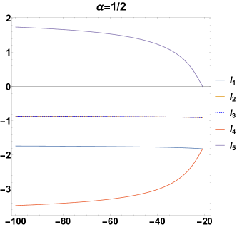
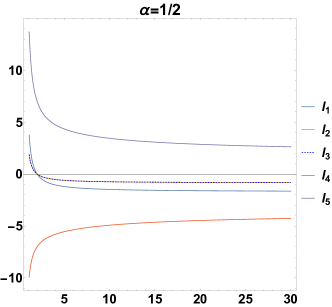
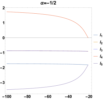
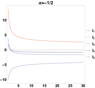
   Figure 1: Real part of the eigenvalues for point $P_{4}$ for $\alpha=\pm\frac{1}{2}$ and different ranges for $\lambda$ where the point exists.

7. $P_{5}=(\Omega_{R},y,\Sigma,x,z)=(\frac{6\lambda+6}{5-7\lambda},\frac{\sqrt{6}\sqrt{\lambda(\lambda+20)-17}}{5-7\lambda},-\frac{2(\lambda-2)}{7\lambda-5},\frac{18}{5-7\lambda},0).$ The difference with $P_{4}$ is a minus sign in the $y$ coordinate, it exists for the same values of $P_{4}$ as well. The stability is also the same (saddle) since they share eigenvalues see FIG. 1 for reference. The value of the deceleration parameter is $q(P_{5})=\frac{2(\lambda-2)}{7\lambda-5},$ $P_{5}$ describes an accelerated solution for $\frac{5}{7}<\lambda<2$ and a de Sitter solution for $\lambda=1.$

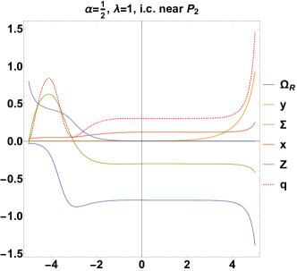
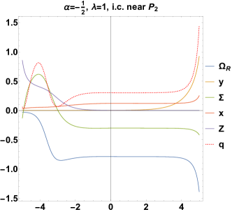
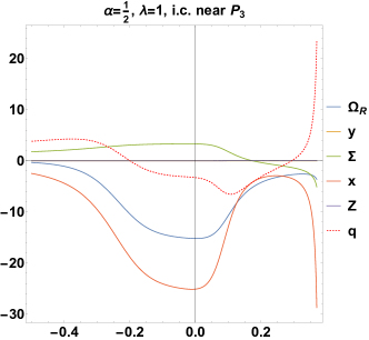
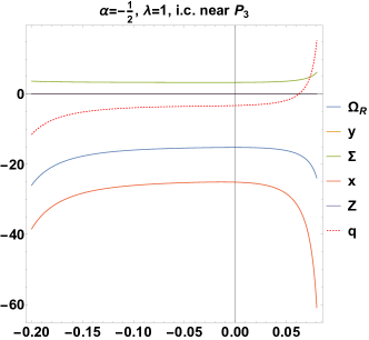
Figure 2: Evolution of $\Omega_{R},y,\Sigma,x,Z$ evaluated at a numerical solutions of system (37)-(V) for $\alpha=\pm\frac{1}{2}$ and $\lambda=1$ for initial conditions (i.c.) near the points $P_{2}$ and $P_{3}$ with a displacement of $\epsilon=\frac{1}{1000}.$ Also present as a red dotted line is the evolution of the deceleration parameter $q$ evaluated at these points.

V.1 General case

For the general case with $\alpha$ arbitrary, we introduce the dimensionless variables

$$\begin{split}&\Omega_{R}=\frac{ke^{b-2\int H\,dt}}{3H^{2}},\quad y^{2}=\frac{V(\phi)}{6H^{2}\phi},\quad\Sigma^{2}=\frac{\dot{b}^{2}}{4H^{2}},\quad x=\frac{\dot{\phi}}{H\phi},\\ &z=\frac{\dot{\Psi}}{H},\quad w=\frac{\beta\dot{\phi}e^{-2b-2\int H\,dt}}{6H^{2}\phi\dot{\Psi}}.\end{split}$$ (42)

In these variables, the Friedmann equation reads

$$\frac{(k-2\alpha)^{2}xz}{24\alpha}-\frac{x\Omega_{R}}{kz}-\Sigma^{2}-w+y^{2}+\Omega_{R}+1=0.$$ (43)

This means that we can solve (43) for $w$ to obtain the dynamical system

$$\Omega_{R}^{\prime}= \frac{x\Omega_{R}\left(12\alpha-(k-2\alpha)^{2}z\right)}{6\alpha}+2\Omega_{R}\left(2\Sigma^{2}+\Sigma+y^{2}\right),$$ (44)

$$y^{\prime}= \frac{xy\left(6\alpha(\lambda+1)-(k-2\alpha)^{2}z\right)}{12\alpha}+y\left(2\Sigma^{2}+y^{2}+1\right)$$ (45)

$$\Sigma^{\prime}= -\frac{(k-2\alpha)^{2}(\Sigma-1)xz}{12\alpha}-\frac{3x\Omega_{R}}{kz}+2(\Sigma-1)^{2}(\Sigma+1)+(\Sigma+2)y^{2}+3\Omega_{R},$$ (46)

$$\begin{split}\left(-\Sigma^{2}+y^{2}+\Omega_{R}+1\right)z^{\prime}&=z\left(-2(\Sigma-1)^{3}(\Sigma+1)+2\Omega_{R}\left((\Sigma-1)^{2}+x\right)\right)\\ &+z\left(y^{2}((\Sigma-4)\Sigma+(\lambda+1)x+\Omega_{R}+3)+y^{4}\right)\\ &-\frac{(k-2\alpha)^{2}}{12\alpha}xz^{2}\left(-(\Sigma-1)^{2}+y^{2}+\Omega_{R}\right)+\frac{6}{k}\Sigma x\Omega_{R},\end{split}$$ (47)

$$\begin{split}\frac{12\alpha z}{x}&\left(-\Sigma^{2}+y^{2}+\Omega_{R}+1\right)^{2}x^{\prime}=-(k-2\alpha)^{2}xz^{2}\left(x\left(\Sigma^{2}+\lambda y^{2}+\Omega_{R}-1\right)\right)\\ &+(k-2\alpha)^{2}xz^{2}\left(\left(-(\Sigma-6)\Sigma+y^{2}+\Omega_{R}-5\right)\left(-\Sigma^{2}+y^{2}+\Omega_{R}+1\right)\right)\\ &-\frac{6z}{k}\left((k-2\alpha)^{2}\Sigma x^{2}\Omega_{R}\right)\\ &-6z\left(4\alpha x\left(-\Sigma^{2}+y^{2}+\Omega_{R}+1\right)\left(\Sigma^{2}+\lambda y^{2}+\Omega_{R}-1\right)\right)\\ &-\frac{6z}{k}\left(2\alpha k\left(2(\Sigma-1)^{2}+y^{2}\right)\left(-\Sigma^{2}+y^{2}+\Omega_{R}+1\right)^{2}\right)\\ &+\frac{(k-2\alpha)^{4}}{6\alpha}(\Sigma-1)x^{2}z^{3}-\frac{72\alpha\Sigma}{k}x\Omega_{R}\left(-\Sigma^{2}+y^{2}+\Omega_{R}+1\right),\end{split}$$ (48)

where once more the prime means a total derivative with respect the independent variable $\tau=\ln(a)$.

The equilibrium points for the latter system are given by the family $(\Omega_{R},y,\Sigma,x,z)=(0,0,\Sigma_{c},\frac{24\alpha\left(\Sigma_{c}^{2}-1\right)}{(k-2\alpha)^{2}z_{c}},z_{c})$ where $\Sigma_{c}~{}$and $z_{c}\in\mathbb{R}$ are the parameters that define the family. This family is a normally hyperbolic set of equilibrium points and therefore it has two zero eigenvalues. We observe that there are not any asymptotic solutions which can describe anisotropic solutions with nonzero spatial curvature, that is, the limit of GR is not recovered in this case.

We conclude that the general case is not of physical interest, thus we end the discussion here.

VI Concluding remarks

In this study we investigated the asymptotic dynamics for the field equations in symmetric teleparallel $f\left(Q\right)$-theory for Kantowski-Sachs and Bianchi type III background geometries. The field equations of $f\left(Q\right)$-theory are of second-order where the geometrodynamical degrees of freedom can be attributed to two scalar fields. By using the scalar field description we were able to write a minisuperspace Lagrangian. From the minisuperspace approach we observed that, for specific values of some of the free parameters of theory, some nonlinear terms in the field equations are eliminated.

To understand the overall evolution of physical parameters in the solution space, we determined the stationary points of the phase-space and investigated their stability properties. Employing the Hubble normalization approach, we transformed the field equations into a system of algebraic-differential equations. Each stationary point of this system corresponded to an asymptotic solution, whose stability properties and physical characteristics we thoroughly examined.

We found that for the general form of the symmetric and teleparallel connection provided by the theory, the field equations admit asymptotic solutions describing dynamics similar to that of the Bianchi type I geometry, without recovering the limit of General Relativity (GR). However, for specific values of the free parameters, new stationary points emerged, describing the limit of GR and potentially representing anisotropic and accelerated solutions that could describe the pre-inflationary epoch of the universe.

From the results of this work it follows that symmetric teleparallel $f\left(Q\right)$-theory can describe anisotropic solutions with acceleration. However, we have considered a power-law function for the $f\left(Q\right)$-only and we have not found any future attractor which can describe an accelerating universe. However, for a more general $f\left(Q\right)$ function, new stationary points exist. Finally, we demonstrated how the phase-space analysis can be utilized to constrain the free parameters of the connection, in order to ensure the viability of the theory.

Data Availability Statements: Data sharing is not applicable to this article as no datasets were generated or analyzed during the current study.

References

• (1) N. Aghanim et al. [Planck], Astron. Astrophys. 641 (2020), A6 [erratum: Astron. Astrophys. 652 (2021), C4] doi:10.1051/0004-6361/201833910 [arXiv:1807.06209 [astro-ph.CO]].
• (2) N. Aghanim et al. [Planck], Astron. Astrophys. 641 (2020), A1 doi:10.1051/0004-6361/201833880 [arXiv:1807.06205 [astro-ph.CO]].
• (3) A. G. Riess, S. Casertano, W. Yuan, L. M. Macri and D. Scolnic, Astrophys. J. 876 (2019) no.1, 85 doi:10.3847/1538-4357/ab1422 [arXiv:1903.07603 [astro-ph.CO]].
• (4) M. A. Troxel et al. [DES], Phys. Rev. D 98 (2018) no.4, 043528 doi:10.1103/PhysRevD.98.043528 [arXiv:1708.01538 [astro-ph.CO]].
• (5) C. Hikage et al. [HSC], Publ. Astron. Soc. Jap. 71 (2019) no.2, 43 doi:10.1093/pasj/psz010 [arXiv:1809.09148 [astro-ph.CO]].
• (6) C. Heymans, T. Tröster, M. Asgari, C. Blake, H. Hildebrandt, B. Joachimi, K. Kuijken, C. A. Lin, A. G. Sánchez and J. L. van den Busch, et al. Astron. Astrophys. 646 (2021), A140 doi:10.1051/0004-6361/202039063 [arXiv:2007.15632 [astro-ph.CO]].
• (7) H. Hildebrandt, J. L. Van Den Busch, A. H. Wright, C. Blake, B. Joachimi, K. Kuijken, T. Tröster, M. Asgari, M. Bilicki and J. T. A. De Jong, et al. Astron. Astrophys. 647 (2021), A124 doi:10.1051/0004-6361/202039018 [arXiv:2007.15635 [astro-ph.CO]].
• (8) M. Asgari et al. [KiDS], Astron. Astrophys. 645 (2021), A104 doi:10.1051/0004-6361/202039070 [arXiv:2007.15633 [astro-ph.CO]].
• (9) T. Tröster et al. [KiDS], Astron. Astrophys. 649 (2021), A88 doi:10.1051/0004-6361/202039805 [arXiv:2010.16416 [astro-ph.CO]].
• (10) C. García-García, J. R. Zapatero, D. Alonso, E. Bellini, P. G. Ferreira, E. M. Mueller, A. Nicola and P. Ruiz-Lapuente, JCAP 10 (2021), 030 doi:10.1088/1475-7516/2021/10/030 [arXiv:2105.12108 [astro-ph.CO]].
• (11) E. Di Valentino, O. Mena, S. Pan, L. Visinelli, W. Yang, A. Melchiorri, D. F. Mota, A. G. Riess and J. Silk, Class. Quant. Grav. 38 (2021) no.15, 153001 doi:10.1088/1361-6382/ac086d [arXiv:2103.01183 [astro-ph.CO]].
• (12) G. Efstathiou, Mon. Not. Roy. Astron. Soc. 505 (2021) no.3, 3866-3872 doi:10.1093/mnras/stab1588 [arXiv:2103.08723 [astro-ph.CO]].
• (13) D. S. Goldwirth and T. Piran, Phys. Rev. Lett. 64 (1990), 2852-2855 doi:10.1103/PhysRevLett.64.2852
• (14) Misner, C. W., Thorne, K. S., and Wheeler, J. A. Gravitation. 1973.
• (15) Peebles, P., and Peebles, P.Principles of Physical Cosmology. Princeton Series in Physics. Princeton University Press, 1993.
• (16) G.F.R. Ellis and M.A.H. MacCallum, Comm. Math. Phys. 12, 108 (1969)
• (17) M. Goliath and G.F.R. Ellis, Phys. Rev. D 60, 023502 (1999)
• (18) M. Le Delliou, M. Deliyergiyev and A. del Popolo, Symmetry 12 (2020) no.10, 1741 doi:10.3390/sym12101741
• (19) P. Fosalba and E. Gaztanaga, doi:10.1093/mnras/stab1193 [arXiv:2011.00910 [astro-ph.CO]].
• (20)  C.W. Misner, Astroph. J. 151, 431 (1968)
• (21) C.W. Misner, Phys. Rev. Lett. 22, 1071 (1969)
• (22) N. Cornish and J. Levin, Phys. Rev. D 55, 7486 (1997)
• (23) M.P. Ryan and L.C. Shepley, Homogeneous Relativistic Cosmologies, Princeton University Press (1975)
• (24) J. Wainwright and G. F. R. Ellis, Dynamical Systems in Cosmology, Cambridge University Press (1997)
• (25) R. Kantowski and R.K. Sachs, J. Math. Phys. 7, 443 (1966)
• (26) J.M. Nester an H.-J. Yo, Chin. J. Phys. 37, 113 (1999)
• (27) J.B. Jimenez, L. Heisenberg and T. Koivisto, Phys. Rev. D 98, 044048 (2018)
• (28) A.G. Riess et al., Astron. J. 116, 1009 (1998)
• (29) M. Tegmark et al., Astrophys. J. 606, 702 (2004)
• (30) E. Komatsu et al., Astrophys. J. Suppl. Ser. 180, 330 (2009)
• (31) N. Suzuki et al., Astrophys. J. 746, 85 (2012)
• (32) L. Heisenberg, Phys. Reports 796, 1 (2019)
• (33) J.B. Jimenez, L. Heisenberg, T. Koivisto and S. Pekar, Phys. Rev. D 101, 103507 (2020)
• (34) H.A. Buchdahl, Mon. Not. Roy. Astron. Soc. 150, 1 (1970)
• (35) R. Ferraro and F. Fiorini, Phys. Rev. D 75, 084031 (2007)
• (36) R. Weitzenböck, Invarianten Theorie, Nordhoff, Groningen (1923)
• (37) T. Clifton, P.G. Ferreira, A. Padilla and C. Skordis, Phys. Reports 513, 1 (2012)
• (38) S. Nojiri, S.D. Odintsov and V.K. Oikonomou, Phys. Reports 692, 1 (2017)
• (39) S. Capozziello, Int. J. Mod. Phys. D 11, 483 (2002)
• (40) L. Atayde and N. Frusciante, Phys. Rev. D 104, 064052 (2021)
• (41) F. K. Anagnostopoulos, S. Basilakos and E. N. Saridakis, Phys. Lett. B 822, 136634 (2021)
• (42) J. Shi, Eur. Phys. J. C 83, 951 (2023)
• (43) O. Sokoliuk, S. Arora, S. Praharaj, A. Baransky and P.K. Sahoo, Mon. Not. Roy. Astron. Soc. 522, 252 (2023)
• (44) A. Lymperis, Late-time cosmology with phantom dark-energy in f(Q) gravity, JCAP 11, 018 (2022)
• (45) G.K. Goswami, Rita Rani, J.K. Singh and A. Pradhan, An FLRW accelerating universe model in Weyl type f(Q) gravity and Observational Constraints, (2023) [arXiv:2309.01233]
• (46) A. De and T.-H. Loo, Class. Quantum Grav. 40, 115007  (2023)
• (47) N. Dimakis, M. Roumeliotis, A. Paliathanasis, P.S. Apostolopoulos and T. Christodoulakis, Phys. Rev. D 106, 123516 (2022)
• (48) A. Paliathanasis, Phys. Dark Univ. 41, 101255 (2023)
• (49) H. Shabani, A. De and T.-H. Loo, Eur. Phys. J. C 83, 535 (2023)
• (50) K. Hu, T. Katsuragawa and T. Qiu, Phys. Rev. D 106, 044025 (2022)
• (51) F. D.’ Ambrosio, L. Heisenberg and S. Zentara, Hamiltonian Analysis of f(Q) Gravity and the Failure of the Dirac–Bergmann Algorithm for Teleparallel Theories of Gravity, (2023) [arXiv:2308.02250]
• (52) K. Tomonari and S. Bahamonte, Dirac-Bergmann analysis and Degrees of Freedom of Coincident f(Q)-Gravity (2023) [arXiv:2308.06469]
• (53) N. Dimakis, A. Paliathanasis and T. Christodoulakis, Class. Quantum Grav. 38, 225003 (2021)
• (54) N. Dimakis, A. Paliathanasis and T. Christodoulakis, Phys. Rev. D 109, 024031 (2024)
• (55) R. Zia, D.C. Maurya and A.K. Shukla, Int. J. Geom. Meth. Mod. Phys. 18, 2150051 (2021)
• (56) S. Capozziello, V. De Falco and C. Ferrara, The role of the boundary term in f(Q,B) symmetric teleparallel gravity, (2023) [arXiv:2307.1320]
• (57) T.-H. Loo, M. Koussour and A. De, Annals Phys. 454, 169333 (2023)
• (58) L. Atayde amd N. Frusciante, Phys. Rev. D 107, 124048 (2023)
• (59) M. Koussour and A. De, Eur. Phys. J. C 83, 400 (2023)
• (60) S. Capozziello, V. De Falco and C. Ferrara, Eur. Phys. J. C 82, 865 (2022)
• (61) K.F. Dialektopoulos, T.S. Koivisto and S. Capozziello, Eur. Phys. J. C 79, 606 (2019)
• (62) L.P. Eisenhart, Non-Riemannian Geometry, Dover Books on Mathematics, Dover Publications (2012)
• (63) M. Hohmann, General covariant symmetric teleparallel cosmology, Phys. Rev. D 104 124077 (2021)
• (64) F. D’ Ambrosio, L. Heisenberg and S. Kuhn, Revisiting cosmologies in teleparallelism, Class. Quantum Grav. 39 025013 (2022)
• (65) D. Zhao, Covariant formulation of f(Q) theory, Eur. Phys. J. C 82, 303 (2022)
• (66) S. Bahamonte and L. Järv, Eur. Phys. J. C 82, 963 (2022)
• (67) A. Paliathanasis, N. Dimakis and T. Christodoulakis, Phys. Dark Univ. 43, 101410 (2024)
• (68) N. Dimakis, M. Roumeliotis, A. Paliathanasis and T. Christodoulakis, Eur. Phys. J. C 83, 794 (2023)
• (69) S. Bahamonde, K. F. Dialektopoulos, C. Escamilla-Rivera, G. Farrugia, V. Gakis, M. Hendry, M. Hohmann, J. Levi Said, J. Mifsud and E. Di Valentino, Rept. Prog. Phys. 86 (2023) no.2, 026901 doi:10.1088/1361-6633/ac9cef [arXiv:2106.13793 [gr-qc]].
• (70) L. Heisenberg, [arXiv:2309.15958 [gr-qc]].