Concurrent Speaker Detection: A multi-microphone Transformer-Based Approach

Abstract

We present a deep-learning approach for the task of Concurrent Speaker Detection (CSD) using a modified transformer model. Our model is designed to handle multi-microphone data but can also work in the single-microphone case. The method can classify audio segments into one of three classes: 1) no speech activity (noise only), 2) only a single speaker is active, and 3) more than one speaker is active. We incorporate a Cost-Sensitive (CS) loss and a confidence calibration to the training procedure. The approach is evaluated using three real-world databases: AMI, AliMeeting, and CHiME 5, demonstrating an improvement over existing approaches.

I Introduction

Speaker detection, namely the ability to identify and track the activities of individual speakers in an audio stream, is an important task with many practical applications. In particular, Concurrent Speaker Detection (CSD) is the problem of identifying speakers’ presence and overlapping activity in a given audio signal. It classifies audio segments into three classes, namely: 1) no speech activity (noise only), 2) only a single speaker is active, and 3) more than one speaker is active. A reliable CSD is a key component in audio scene analysis and speech processing applications, e.g., speech detection, speaker counting and diarization, and multi-microphone spatial processing in “cocktail party” scenarios. CSD is a challenging task due to the complex nature of human speech. Accent, pitch, and speaking style variations can make the identification and detection of the speakers’ activity challenging. Consequently, developing effective CSD approaches is an active area of research, aiming to improve accuracy and robustness.

In [1], a multichannel CSD, based on Convolutional Neural Networks (CNN) architecture, was used as a building block of a Linearly Constrained Minimum Variance (LCMV) beamformer for controlling the estimation of its components, based on the speakers’ activity patterns. Specifically, the spatial correlation matrix of the noise is estimated during noise-only segments, and the steering vectors of the beamformer are estimated during single active speaker segments. The beamformer’s weights are not updated during concurrent activities of more than one speaker. In [2, 3], both CNN and attention mechanisms are employed for speaker-counting and identification. In [4, 5], a Long Short-Term Memory (LSTM) model is used for the task of Overlapped Speech Detection (OSD). Unlike the CSD, only two classes comprise the OSD task. The first comprises noise-only or single-speaker segments, while the second comprises overlapped speech segments, namely two or more concurrent speakers.

The Transformer model, which was originally proposed in the Natural Language Processing (NLP) domain [6, 7], was later adopted by the audio community for various tasks, e.g., speech separation [8] and audio classification [9]. It was demonstrated in [9] that the Audio Spectrogram Transformer (AST) model, which is an adaptation of the Vision Transformer (ViT) model [10], outperforms CNN-based models. We stress that the AST model only processes single-microphone data, whereas multiple microphones are available in many real-world use cases. It is well-known that, if properly utilized, the additional spatial information may improve performance. In [11], a model based on Temporal Convolutional Networks (TCN) is used, and in [12], a Transformer-based model is used. Both models estimate the activity of the speakers. Specifically, two related tasks are implemented, Voice Activity Detection (VAD) and OSD, as well as their joint estimation. The VAD classifies audio segments into two classes: 1) no active speaker and 2) speech activity (either one or more speakers). We can therefore refer to the combined VAD and OSD task as a CSD task. A Transformer-based solution is also utilized for audio OSD [13] and for audio-visual OSD [14]. The CSD, which is a multi-class classification task, is more complex than OSD or VAD, which are binary classification tasks.

In the current contribution, we propose an algorithm to solve the CSD task. Our contribution is threefold: 1) we extend the use of ViT and adapt it to the multi-microphone case, 2) we incorporate in the training process a re-weighting mechanism according to the importance of each class and further use calibration to improve the classification accuracy, and finally 3) similarly to [11, 12, 14, 4, 13, 5], we evaluate the performance of the proposed model on AMI [15] and CHiME 5 [16] databases, and additionally on the recently introduced AliMeeting [17] database (in Chinese).

II Problem Formulation

Let $X_{i}(\ell,k),\,i=1,\ldots,N$ represent the Short-Time Fourier Transform (STFT) of the microphone signals, where $N$ is the number of microphones, $\ell$ and $k$ represent the frame index and the frequency index, respectively. The goal of a CSD algorithm is to classify each audio segment (either single-microphone or multi-microphone) into one of the three classes:

$$\mathrm{CSD}(\ell)=\begin{cases}\textrm{Class \#0}&\textrm{Noise only}\\ \textrm{Class \#1}&\textrm{Single-speaker activity}\\ \textrm{Class \#2}&\textrm{Concurrent-speaker activity}\end{cases}.$$ (1)

The statistical characteristics of the audio segments may change according to the scenario. Multiple types of noise may exist for class ‘0’ (‘Noise-Only’). Class ‘1’ (‘Single-speaker activity’) can be challenging due to the variability of human speech. Individuals may have different accents, speaking styles, and vocal characteristics, making it difficult for algorithms to identify them accurately. In class ‘2’ (‘Concurrent-speaker activity’), the different number of active speakers may result in diverse statistical properties. In addition, the presence of background noise or reverberation can further complicate the task. Consequently, developing robust and accurate CSD methods that can handle a wide range of input conditions becomes essential.

III Proposed Model

The proposed CSD model is based on the ViT [10] architecture, which has achieved state-of-the-art performance on a variety of computer vision tasks. We have modified the original ViT architecture to better suit audio processing requirements, including the use of log-spectrum as input and the ability to handle both single-channel and multichannel audio. The input features are the log-magnitude of the STFT of the audio signals, denoted hereinafter log-spectrum.

The model consists of three main blocks: Embedding, Transformer, and Classification. The first block linearly projects the input data and generates the input tokens for the Transformer model. The second block is a multi-head attention (MHA) transformer block, consisting of self-attention layers, which can capture complex relations within its input data. The attention mechanism [7] allows the model to simultaneously focus on different parts of the input, enabling it to learn rich feature representations from the log-spectrum. Finally, several fully-connected layers are applied to map the learned features to the final output predictions.

Our starting point is, therefore, the ViT model, with the images substituted by the log-spectra and the RGB channels by the multi-microphone measurements. The multichannel model attends to different areas in the input to achieve the best classification results. We use a Cross-Entropy (CE) loss function for training, a common choice for classification tasks. In addition, we used Label-Smoothing (LS) [18] and the Cost-Sensitive (CS) loss function [19] as regularization techniques to improve the ability of the model to generalize to unknown data. The high-level architecture of the model is presented in Fig. 1.

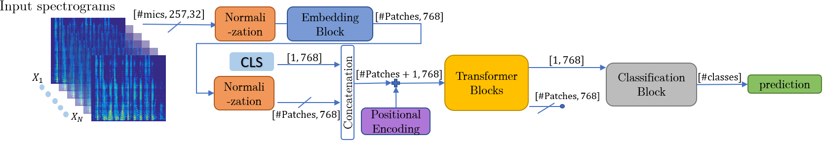
Figure 1: High-level architecture of the proposed model.

III-A Pre-Processing and Input Features

The microphone signals are first resampled to 16kHz (if the original sampling rate differs from the nominal one). Subsequently, the signals are analyzed by an STFT with Hann window of length 512 and 50% overlap. Finally, the log-spectrum is calculated, resulting in 257 frequency bins per frame.

The output labels are determined using the transcribed databases, with a resolution of 0.1 Sec and context frames 0.2 Sec long on both sides of the analyzed segment. Therefore, each audio segment, lasting 0.5 seconds, is categorized into one of the three classes. The overall dimensions of the input tensor are $N\times 257\times 32$, where $N$ is the number of microphones, $257$ is the number of frequency bins, and $32$ is the number of time bins.

III-B Architecture

We will now elaborate on the three blocks comprising the model’s architecture.

The Embedding block receives the input log spectrum and produces the tokens utilized by the Transformer block. This block splits the input data into patches and linearly projects each to form tokens. We set the dimensions of a 2-D learnable kernel and strides values in the Time-Frequency (TF) axes, such that each patch is projected to an embedding space with a dimension $D$ and considered a token. This process results in a features tensor with dimensions $\#\textrm{Tokens}\times D$. This block can be designed to handle both multichannel and single-channel signals, as will be explained below. Following [20], we apply a dual patch-normalization for improving the ViT results (see the ‘Normalization’ block in Fig. 1).

The Transformer block follows the ViT architecture with minor modifications. The Transformer was initialized with random weights and trained with the chosen databases. This module consists of several layers of MHA blocks. We followed the ViT architecture and used Class token [CLS], an additional learnable token added as an input to the Transformer. In addition, a learnable positional embedding is added to each input token before the first MHA layer. In total, the input and output of each MHA blocks are tokens of shape $(\#\textrm{Tokens}+1)\times D$.

The last block in our model, the Classification block, consists of two fully connected layers that map the Transformer output to fit the number of classes. The Classification block takes only the token corresponding to [CLS] as input. This should make the classification process unbiased towards any particular token, as discussed in [10].

III-C Single- and multichannel Embedding Blocks

The Embedding block transforms the input data into tokens used by the Transformer block, comprising 12 Transformers. We stress that the AST model [9] addresses a different classification task and is limited to single-channel inputs. Since we are also interested in the multichannel case, the standard embedding block should be modified accordingly.

The basic, single-microphone structure, i.e. $N=1$, is depicted in Fig. 2(a). The input log spectrum is split into patches with a 2-D learnable kernel with a stride set to 1. In ViT, the shape of the patches is $16\times 16$, but according to our analysis, a more useful patch size is $257\times 8$, as it jointly analyzes the entire frequency axis. Later on, each patch is linearly projected to a dimension of $D=768$, resulting in a tensor of shape $\#\textrm{Patches}\times 768$.

The information must be merged from the different channels for the multichannel case. The overall proposed structure is depicted in Fig. 2(b). The most effective merging technique, denoted here as Type #1, entails independently applying a single-channel embedding to each microphone signal and then combining all channels through concatenation. This process yields an output tensor with dimensions $N\cdot\#\textrm{Patches}\times 768$. Ensuring identical channel numbers during both the training and testing stages is necessary for this structure. Furthermore, due to the expansion of the channel dimension compared to the single-microphone scenario, there is an increase in the number of input tokens for the subsequent Transformer block. Similarly, the input feature vector to the Classification block also increases. All of which increase the total number of parameters.

To further analyze the merging strategies, we have examined two alternatives, designated hereinafter Type #2 and Type #3.

In Type #2, each single-channel embedding block is independently applied, and a summation operation merges the information. The resulting data shape is $\#\textrm{Patches}\times 768$. While the independent processing of each channel may be beneficial performance-wise, it also requires the number of channels to be identical in the training and test stages.

In Type #3, the weights of all single-channel embedding blocks are shared (Siamese networks), and their output is then merged using an averaging operation. The shape of the result is again $\#\textrm{Patches}\times 768$. This structure is indifferent to a mismatch between the number of microphones in the training and test stages and simultaneously reduces the number of parameters. Nevertheless, it may fall short of fully capturing the relationships between the signals from the microphones.

After experimenting with all three alternatives, we decided to use Type #1 due to its ability to perform cross-channel attention, a property that enhances the overall performance of the proposed method. Table I compares the mean average precision (mAP) results for the three merging types for all databases. Table I further supports choosing Type #1 since it outperforms all three types for the OSD task while exhibiting only marginal performance degradation for the VAD task.

TABLE I: Ablation study for merging strategies: The mean average precision (mAP) (%) measure for the VAD and the OSD classifiers, as well as the number of required parameters (#P) in millions (M).

	AMI			AliMeeting			CHiME
	VAD	OSD	#P (M)	VAD	OSD	#P (M)	VAD	OSD	#P (M)
Type #1	98	73.1	98.1	98.2	87.8	98.1M	91.6	83.5	91.8
Type #2	98.1	69.5	98.1	99.6	73.8	98.1M	96.6	56.5	91.7
Type #3	97.9	71.9	86.9	98.3	86.4	86.9M	91.9	63.4	86.9

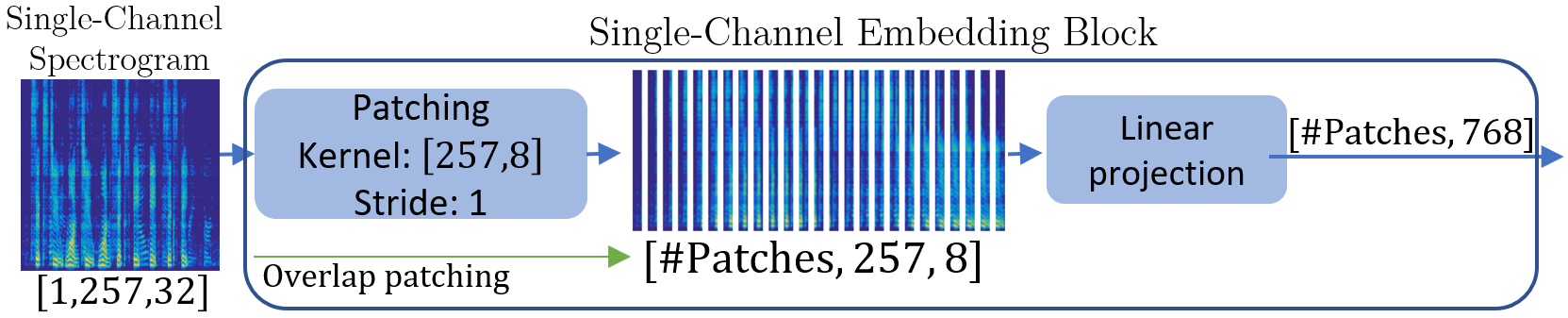
(a) Single-Channel Embedding Block: Embedding layer for a single-channel log-spectrum.

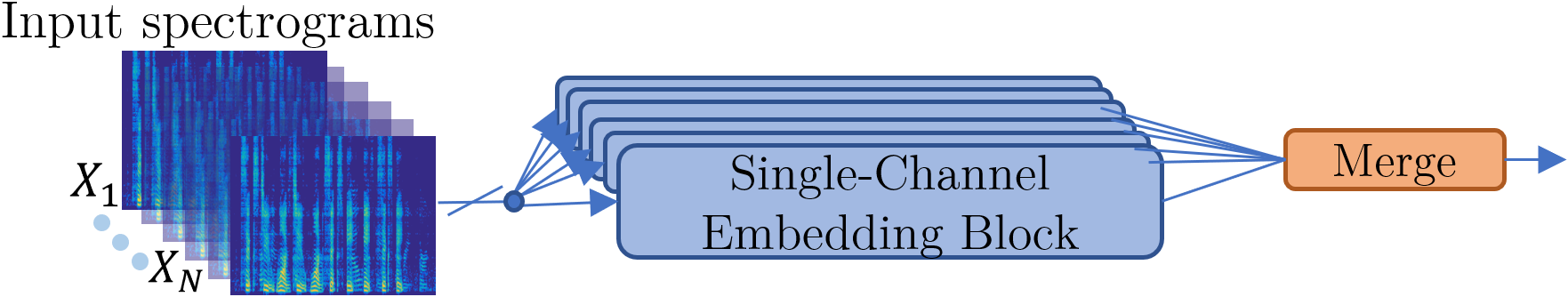
(b) multichannel Embedding Block: The ‘merge’ operation stands for either summation, averaging, or concatenation. All ‘single channel blocks’ weights can be either shared or distinct.

Figure 2: Embedding Block: Details.

III-D Objective Functions

As we aim at the classification task, the natural choice for a loss function is the Cross-Entropy (CE). However, the classification results were not balanced between the different classes in our databases. We have, therefore, used two additional methods to guide the model to focus on the more challenging examples in the data, mainly Class #1. We used Label-Smoothing (LS) [18] and class weights. Both demonstrated an improvement in classification accuracy. We also applied the Cost-Sensitive (CS) loss [19]. In this procedure, we follow a 2-stage training procedure: First, we train the model with no CS loss, then we modify the CS loss weights according to the results and retrain the model. The CS loss weights are defined as a $3\times 3$ matrix that gives more weight, i.e., increasing the loss function, for more frequent classification errors. When applying the CS loss, we use an extra hyper-parameter weighting between the CS loss and the CE loss. This hyper-parameter was tested extensively and was set to a value of 15-20 (depending on the different databases).

III-E Confidence Calibration

After training the model, we applied confidence calibration using temperature scaling [21]. The model calibration can become handy when the model is used to control the estimation of the building blocks of a beamformer [1], where erroneous classification can significantly deteriorate the separation performance. Calibration enhances the interpretability of the model’s predictions by aligning them with probabilities, establishing an appropriate threshold for considering the prediction valid. An instance of utilizing a calibrated model involves setting segments with predictions below a certain threshold to Class #2. These segments are then excluded from the estimation of the beamformer’s weights.

IV Experimental study

IV-A Databases

We applied the proposed model to three real-world databases, namely AMI [15], AliMeeting [17], and CHiME 5 [16]. All databases use a microphone array for the recordings, AMI and AliMeeting use an 8-microphone array, and CHiME 5 uses a 4-microphone array. AMI database consists of 100 hours of meeting recordings with English speakers (both male and female) in 3 different rooms and setups. The AliMeeting comprises 118.75 hours of real meetings with 2-4 participants speaking in Mandarin. The CHiME 5 database consists of recordings of conversations between English speakers from different real-home environments. CHiME 5 has six arrays (U01 to U06) with four microphones each. We chose to train and report only for arrays U01 and U02.

All databases are fully transcribed with phrase-level resolution. This allows us to generate ground-truth labels for training the model. The distribution of the different classes is depicted in Table II, where it is evident that the classes are unbalanced. The phrases are dominated by Class #1, as typical to natural human conversations. This imbalance between the different classes must be addressed during training to avoid biased classification results. This is done by modifying the cost function during training, as elaborated above.

TABLE II: Class frequency [%] in all databases.

Database/Class	#0	#1	#2
Ali-Meeting	6.9	67.2	25.9
AMI	16.8	71.8	11.4
CHiME 5	20.5	50.9	28.6

We split the databases into train, validation, and test sets.

CHiME 5 database: We used the existing Train-Val-Test split given on the challenge’s official website. Note that we chose to remove all utterances with saturated sound files. We demonstrated our results using only U01 and U02, while [12] uses all arrays U01-U06 and presents the average results.

AMI and AliMeeting databases: We used the official Train-Val-Test splits as provided in the databases’ documentation.

IV-B Algorithm Setup

We used the architecture described in Section III-C with Type #1 Embedding block and CS loss for all models since, as discussed above, it stands out as the most effective scheme. In training the models, we used the Adam optimizer with a learning rate of $1e^{-6}$, a weight decay of $1e^{-9}$, and a batch size of 128. To prevent overfitting, considering the model’s substantial parameter count, we limit the number of epochs to a range of 10-15, depending on the examined database. The overall parameter count falls within the range of 86.9-98.1M, as illustrated in Table I. We used the following hyperparameters: The Embedding block is set with a dimension of $D=768$, and the Transformer block is set with 12 heads and a depth of 12. The classification block has one hidden layer with dimension 387.

IV-C Results

Choosing the right evaluation metric is essential because our model should classify between three classes. In this work, especially when compared to competing methods, we will evaluate the performance of the proposed scheme in terms of Precision, Recall, and mean average precision (mAP). To gain further insights into the proposed method’s performance and give a more detailed analysis of the errors, we also chose to present the confusion matrix that compares the ground-truth labels with the predicted labels by our model (as a percentage normalized to the ground-truth labels). The confusion matrices for the single-microphone case are depicted in Table III and Table IV for the multi-microphone case.

TABLE III: CSD results: Single-microphone model confusion matrices, as [%] normalized to the ground-truth labels. ‘T’-true labels, ‘P’-predicted labels.

	AMI			AliMeeting			CHiME
T \P	0	1	2	0	1	2	0	1	2
0	78	20	2	88	11	1	55	32	13
1	9	75	16	10	77	13	10	51	39
2	1	37	62	2	30	68	3	34	63

TABLE IV: CSD results: Multi-microphone model confusion matrices, as [%] normalized to the ground-truth labels. Using the Type #1 embedding block. ‘T’-true labels, ‘P’-predicted labels.

	AMI			AliMeeting			CHiME
T \P	0	1	2	0	1	2	0	1	2
0	80	18	2	85	13	2	73	21	6
1	10	74	16	7	82	11	19	51	30
2	2	35	63	2	28	70	8	33	59

A performance comparison, in terms of the Precision, Recall, and mAP (%) metrics for the OSD task for the AMI database is depicted in Table V. We compare both our single- and multichannel variants to several algorithms from the literature [12, 14, 5, 13, 22]. It is worth noting that [14] introduces three models employing distinct modalities for the OSD task: 1) audio-only, 2) video-only, and 3) audiovisual. Our reference pertains to the audio-only model. We emphasize that our multi-class CSD task is inherently more intricate than the binary OSD task. We transformed our CSD classification results into two binary classification tasks to facilitate comparison. This involved combining two classes: for the VAD task, classes #1 and #2 were aggregated, while for the OSD task, classes #0 and #1 were aggregated. Notably, the proposed model demonstrates a significant performance superiority over competing methods in the OSD task.

As outlined in Table VI, a comparison between the proposed multi-microphone model and [12] using the mAP metric reveals a significant improvement in the OSD task. However, there is a slight decrease in performance for the VAD task. The AliMeeting database stands out with the most favorable classification results, while the CHiME database proves to be the most challenging among the three tested databases.

TABLE V: A comparison between the proposed single- and multi-microphone variants and various competing methods in evaluating the performance on the OSD task, including Precision, Recall, and mAP (%) measures on the AMI Database.

Variant	Method	Precision	Recall	mAP
	[12]	N/A	N/A	59.1
Single-channel	[14]	N/A	N/A	62.7
	[5]	86.8	65.8	N/A
	pyannote 2.0 [22]	80.7	70.5	N/A
	Our	91.4	88.9	69.3
	[13]	87.8	87	N/A
multichannel	[12]	87.8	87	60.3
	Our	92.4	89	73.1

TABLE VI: Multi-microphone model: Comparison of mAP (%) for VAD and OSD tasks, tested over all three databases.

	VAD		OSD
	[12]	Ours	[12]	Ours
AMI	98.7	98.7	60.3	73.1
CHiME	95.4	91.6	52.4	83.5
AliMeeting	N/A	98.2	N/A	87.8

V Conclusions

In this paper, we introduced a multi-microphone transformer-based model designed for the CSD task, accompanied by a training scheme capable of assigning weights to classes based on their importance and incorporating a calibration stage. Through experiments, we illustrated the practicality of our proposed model in real-world databases, showcasing its performance advantages compared to existing methods. Notably, the model exhibits versatility, proving effective in both single- and multi-microphone scenarios, with a distinct advantage observed in the latter.

References

- [1] S. E. Chazan, J. Goldberger, and S. Gannot, “LCMV beamformer with DNN-based multichannel concurrent speakers detector,” in 26th European Signal Processing Conference (EUSIPCO), 2018, pp. 1562–1566.
- [2] M. Yousefi and J. H. Hansen, “Real-Time Speaker Counting in a Cocktail Party Scenario Using Attention-Guided Convolutional Neural Network,” in Proc. Interspeech 2021, 2021, pp. 1484–1488.
- [3] N. Kanda, Y. Gaur, et al., “Joint Speaker Counting, Speech Recognition, and Speaker Identification for Overlapped Speech of any Number of Speakers,” in Proc. Interspeech 2020, 2020, pp. 36–40.
- [4] N. Sajjan, S. Ganesh, et al., “Leveraging lstm models for overlap detection in multi-party meetings,” in IEEE International Conference on Acoustics, Speech and Signal Processing (ICASSP), 2018, pp. 5249–5253.
- [5] L. Bullock, H. Bredin, and L. P. Garcia-Perera, “Overlap-aware diarization: Resegmentation using neural end-to-end overlapped speech detection,” in ICASSP 2020 - 2020 IEEE International Conference on Acoustics, Speech and Signal Processing (ICASSP), 2020, pp. 7114–7118.
- [6] A. Gillioz, J. Casas, et al., “Overview of the transformer-based models for NLP tasks,” in 15th Conference on Computer Science and Information Systems (FedCSIS), 2020, pp. 179–183.
- [7] A. Vaswani, N. Shazeer, et al., “Attention is all you need,” Advances in neural information processing systems (NeurIPS), vol. 30, 2017.
- [8] C. Subakan, M. Ravanelli, et al., “Attention is all you need in speech separation,” in IEEE International Conference on Acoustics, Speech and Signal Processing (ICASSP), 2021, pp. 21–25.
- [9] Y. Gong, Y.-A. Chung, and J. Glass, “AST: Audio Spectrogram Transformer,” in Proc. Interspeech, 2021, pp. 571–575.
- [10] A. Dosovitskiy, L. Beyer, et al., “An image is worth 16x16 words: Transformers for image recognition at scale,” in International Conference on Learning Representations (ICLR), 2021.
- [11] S. Cornell, M. Omologo, et al., “Detecting and counting overlapping speakers in distant speech scenarios,” in Proc. Interspeech, Shanghai, China, Oct. 2020.
- [12] ——, “Overlapped speech detection and speaker counting using distant microphone arrays,” Computer Speech & Language, vol. 72, p. 101306, 2022.
- [13] S. Zheng, S. Zhang, et al., “Beamtransformer: Microphone array-based overlapping speech detection,” arXiv preprint arXiv:2109.04049, 2021.
- [14] M. Kyoung, H. Jeon, and K. Park, “Audio-visual overlapped speech detection for spontaneous distant speech,” IEEE Access, vol. 11, pp. 27 426–27 432, 2023.
- [15] J. Carletta, S. Ashby, et al., Machine Learning for Multimodal Interaction. Springer Berlin Heidelberg, 2006, ch. The AMI Meeting Corpus: A Pre-announcement, pp. 28–39.
- [16] J. Barker, S. Watanabe, et al., “The fifth ‘chime’ speech separation and recognition challenge: Dataset, task and baselines,” in Proceedings Interspeech, Hyderabad, India, Sept. 2018.
- [17] F. Yu, S. Zhang, et al., “M2MeT: The ICASSP 2022 multi-channel multi-party meeting transcription challenge,” in IEEE International Conference on Acoustics, Speech and Signal Processing (ICASSP), 2022.
- [18] R. Müller, S. Kornblith, and G. E. Hinton, “When does label smoothing help?” Advances in neural information processing systems (NeurIPS), vol. 32, 2019.
- [19] A. Galdran, J. Dolz, et al., “Cost-sensitive regularization for diabetic retinopathy grading from eye fundus images,” in Medical Image Computing and Computer Assisted Intervention (MICCAI), 2020, pp. 665–674.
- [20] M. Kumar, M. Dehghani, and N. Houlsby, “Dual PatchNorm,” Transactions on Machine Learning Research, 2023.
- [21] C. Guo, G. Pleiss, et al., “On calibration of modern neural networks,” in Proceedings of the 34th International Conference on Machine Learning, vol. 70, Aug. 2017, pp. 1321–1330.
- [22] H. Bredin and A. Laurent, “End-to-end speaker segmentation for overlap-aware resegmentation,” arXiv preprint arXiv:2104.04045, 2021.