Hybrid optimal control with mixed-integer Lagrangian methods

Abstract

Models involving hybrid systems are versatile in their application, but difficult to handle and optimize efficiently due to their combinatorial nature. This work presents a method to cope with hybrid optimal control problems which, in contrast to decomposition techniques, does not require relaxing the integrality constraints. Based on the discretize-then-optimize approach, our scheme addresses mixed-integer nonlinear problems under mild assumptions. The proposed numerical algorithm builds upon the augmented Lagrangian framework, whose subproblems are handled using successive mixed-integer linearizations with trust regions. We validate the performance of the numerical routine with extensive investigations using several hybrid optimal control problems from different fields of application. Promising preliminary results are presented for a motion planning task with hysteresis and drag, a Lotka-Volterra fishing problem, and a facility location design problem.

Keywords. Hybrid dynamics, Optimal control, Mixed-integer programming, Augmented Lagrangian.

AMS MSC. 65K05, 90C06, 90C11, 90C30.

1 Introduction

We consider hybrid optimal control problems (OCP), that is, optimization problems involving possibly nonsmooth dynamics, mixed-integer states or controls, or logical constraints. Hybrid OCPs were investigated, e.g., in [19, 14] where hybrid dynamics are modeled with disjunctive programming. An important subclass of hybrid OCPs are mixed-integer OCPs with discrete-valued controls. Numerical methods often use variable time transformations, relaxation, or decomposition techniques, compare [12, 23] and [25, 16, 17, 15, 20] for important recent developments. Such approaches are often tailored to discrete-valued controls and exploit the time dependency.

In this work, we permit more general hybrid OCPs and apply a direct discretization method to transform the dynamic optimization problem into a finite dimensional mixed-integer nonlinear program (MINLP). Our focus is not on the direct discretization method itself, which exists in various versions, compare [13] for an overview, nor on taking advantage of the time structure. We investigate instead the numerical viability of an optimization scheme that handles hybrid features as they stand, namely without relaxing integrality constraints. Details about modelling and discretization of hybrid OCPs are provided in Section 4.

We study a tailored augmented Lagrangian (AL) method for the numerical solution of a class of MINLPs of the following type:

$$\operatorname*{minimize}\quad f(x)$$ (P)

$$\operatorname{subject~{}to}\quad x\in\mathcal{X},\quad c(x)\in\mathcal{C}$$

with $f\colon\mathcal{X}\to\mathbb{R}$ and $c\colon\mathcal{X}\to\mathbb{R}^{m}$ smooth functions, $\mathcal{C}\subset\mathbb{R}^{m}$ a nonempty closed convex set (projection-friendly in practice), and $\mathcal{X}$ a nonempty closed set with a mixed-integer linear (MIL) structure [5]. In particular, we assume $\mathcal{X}$ to be described by linear inequalities and integrality constraints on some variables, that is,

$$\mathcal{X}:=\left\{x\in\mathbb{R}^{n}\,\middle|\,\begin{array}[]{l}Ax=b,~{}x_{\textup{l}}\leq x\leq x_{\textup{u}},\\ x_{i}\in\mathbb{Z}\quad\forall i\in\mathcal{I}\end{array}\right\}$$ (1)

for some matrix $A$, vectors $b$, $x_{\textup{l}}$ and $x_{\textup{u}}$, and index set $\mathcal{I}$. The general template (P) covers hybrid OCPs discretized with arbitrary schemes, and can capture various features such as mixed-integer control inputs, nonsmooth dynamics and state jumps.

In the following, we will partition the decision variables in $x$ into a real-valued vector $u$ and an integer-valued vector $z$, according to their admissible values for $\mathcal{X}$. Furthermore, we consider the following blanket assumptions.

The approach here is to adopt the AL framework to solve the constrained problem (P) through a sequence of simpler subproblems, that is, moving the nonlinear constraints onto the objective. This methodology is motivated by sequential (partially) unconstrained minimization schemes [11], including (shifted) penalty [2] and barrier (or interior point) methods [8], and by the availability of an affordable solver [5] for problems of the form (P) without nonlinear constraints $c(x)\in\mathcal{C}$. In contrast to global optimization algorithms for (P), which often require convexity of the objective and constraint functions and become heuristics otherwise [1], our method does not rely on such convexity assumptions. Therefore, we do not seek global solutions but are content with suboptimal ones as in [21, 10].

The work contributes a solution technique for (discretized) hybrid OCPs based on an affordable safeguarded AL approach with inexact subproblems. A summary of the optimality concept is described in Section 2, while algorithmic details are provided in Section 3. High-dimensional hybrid OCPs are addressed with our method in Section 4, where numerical results demonstrate its efficacy.

2 Optimality Conditions

This section is dedicated to developing suitable solution concepts for (P). First of all, we seek feasible points, namely some $\bar{x}\in\mathcal{X}$ such that $c(\bar{x})\in\mathcal{C}$. Then, a global minimizer $\bar{x}$ for (P) can be readily characterized by

$$\bar{x}\in\mathcal{X},\quad c(\bar{x})\in\mathcal{C},\quad\forall x\in\mathcal{X},\,c(x)\in\mathcal{C}\colon~{}f(\bar{x})\leq f(x).$$

Since we aim at developing an affordable numerical method, possibly at the price of global optimality, we are interested in local optimality notions too. However, as these are sensitive to how neighborhoods are defined, local notions can be weak and fragile in the mixed-integer setting considered here. Indeed, considering simple balls, sufficiently small neighborhoods of feasible points may contain only one integer configuration, making it locally optimal, in a weak sense. To avoid this naive declaration of local optimality, we develop some stronger conditions by constructing neighborhoods based on $\|\cdot\|_{\textup{LP}}$, which is defined as a polyhedral norm of the real-valued components only [5]. For instance, it can take on the forms

$$\|x\|_{\textup{LP}}:={} \sum\{|x_{i}|\,|\,i\notin\mathcal{I}\} \ell_{1}\text{-type},$$ for

$$\text{or}\quad\|x\|_{\textup{LP}}:={} \max\{|x_{i}|\,|\,i\notin\mathcal{I}\} \ell_{\infty}\text{-type}.$$ for

Although not a norm, $\|\cdot\|_{\textup{LP}}$ induces compact neighborhoods according to $\mathbb{B}_{\textup{LP}}(\bar{x},\Delta):=\{x\in\mathbb{R}^{n}\,|\,\|x-\bar{x}\|_{\textup{LP}}\leq\Delta\}$, owing to the boundedness assumption on integer-valued variables. Now, analogously to the “unconstrained” case [5], local minimizers for (P) can be defined as follows.

We now focus on first-order necessary optimality conditions for (P). These should be useful and practical in order to characterize and numerically detect points that are (at least) candidates for global (or local) minimizers [2, Chapter 3].

2.1 Simple constraints

Let us first consider the minimization of some smooth function $\varphi\colon\mathcal{X}\to\mathbb{R}$ over $\mathcal{X}$:

$$\operatorname*{minimize}\quad \varphi(x) \operatorname{over}\quad x\in\mathcal{X}.$$ (2)

Recalling [5], a first-order criticality measure associated to (2) is defined for all $x\in\mathcal{X}$ and $\Delta\geq 0$ by

$$\Psi_{\varphi,\mathcal{X}}(x,\Delta):=\max_{\begin{subarray}{c}w\in\mathcal{X}\\ \|w-x\|_{\textup{LP}}\leq\Delta\end{subarray}}\langle\nabla\varphi(x),x-w\rangle\geq 0.$$ (3)

Then, a first-order optimality concept for (2) is that in the following definition, which also provides an approximate counterpart thereof.

The denomination criticality, in contrast to stationarity, emphasizes that the former notion is in general significantly stronger than the latter [5].

2.2 Difficult constraints

The “unconstrained” notion of Definition 2.2 is useful to characterize solutions of a problem with simple constraints. But what is a “critical point” for a problem such as (P)? We seek a stationarity characterization that resembles, at least in spirit, the so-called Karush-Kuhn-Tucker (or KKT) conditions in nonlinear programming, see e.g. [2, 6].

Let the Lagrangian function $\mathcal{L}\colon\mathcal{X}\times\mathbb{R}^{m}\to\mathbb{R}$ associated to (P) be defined by

$$\mathcal{L}(x,y):=f(x)+\langle y,c(x)\rangle.$$ (4)

From the viewpoint of nonlinear programming, where local minima correspond to saddle points of the Lagrangian functions, we consider the following notion for KKT-like points of (P), building upon Definition 2.2. Related concepts are available in [8, 6, 7].

Notice that KKT criticality demands feasibility since the normal cone $\mathcal{N}_{\mathcal{C}}(c(\bar{x}))$ to $\mathcal{C}$ at $c(\bar{x})$ would be empty otherwise [6]. By (3), the first condition in Definition 2.3 can be rewritten as

$$\min_{\begin{subarray}{c}x\in\mathcal{X}\\ \|x-\bar{x}\|_{\textup{LP}}\leq\Delta\end{subarray}}\langle\nabla f(\bar{x})+c^{\prime}(\bar{x})^{\top}y,x-\bar{x}\rangle=0$$

meaning that the Lagrangian at $\bar{x}$ cannot be (locally) further minimized with respect to $x$ while maintaining MIL feasibility, in the sense of Definition 2.2. Thanks to the $\|\cdot\|_{\textup{LP}}$-localization, this condition is in general stronger than the inclusion $0\in\nabla_{x}\mathcal{L}(\bar{x},y)+\mathcal{N}^{\textup{lim}}_{\mathcal{X}}(\bar{x})$, corresponding to mere stationarity [7], where $\mathcal{N}^{\textup{lim}}_{\mathcal{X}}(\bar{x})$ denotes the limiting normal cone to $\mathcal{X}$ at $\bar{x}$ [6]. Equivalence holds when the set $\mathcal{X}$ is convex, which is not the case as soon as $\mathcal{I}\neq\emptyset$.

Although a detailed theoretical analysis is beyond the scope of this paper, it is plausible (e.g. patterning the arguments in [6, 4]) that all local minimizers of (P) are KKT critical, possibly under some constraint qualifications.

A criterion for numerical termination arises from relaxing criticality and feasibility requirements in Definition 2.3. Analogously to $\varepsilon$-criticality of Definition 2.2, we consider the following concept, akin to those in [8, 6, 4].

3 Algorithmic Framework

Exploiting the fact that the augmented Lagrangian (AL) approach does not rely on smoothness [2, 6], we will employ an AL scheme to seek a numerical solution for (P) under Assumption 1.1. Building upon a sequence of shifted-penalty subproblems, AL algorithms can be described with a nested structure. An outer loop generates a sequence of primal-dual estimates, adapts shifts and penalty parameters, and monitors convergence toward KKT critical points. Then, each subproblem associated to a set of parameters is addressed by an iterative procedure, effectively an inner loop.

Although the AL framework comprises several algorithms and variants [2, 6, 4, 9], all these share a core element: the successive parametric minimization of an AL function. The safeguarded AL scheme for (P) stated in Algorithm 3.1 patterns that of [2, §4.1] and proceeds with a sequence of subproblems of the form

$$\operatorname*{minimize}\quad \mathcal{L}_{\mu}(x,\widehat{y}) \operatorname{over}\quad x\in\mathcal{X}$$ (5)

for some given penalty parameter $\mu>0$ and multiplier estimate $\widehat{y}\in\mathbb{R}^{m}$. Herein, the simple constraints $x\in\mathcal{X}$ are kept implicit, and the AL function with $\mu>0$ and $\widehat{y}\in\mathbb{R}^{m}$ is defined by

$$\mathcal{L}_{\mu}(x,\widehat{y}):={} f(x)+\frac{1}{2\mu}\operatorname{dist}_{\mathcal{C}}^{2}\left(c(x)+\mu\widehat{y}\right)-\frac{\mu}{2}\|\widehat{y}\|^{2},$$ (6)

cf. [4, 7]. Feasibility of (5) follows from $\mathcal{X}$ being nonempty whereas well-posedness is due to continuity of $\mathcal{L}_{\mu}(\cdot,\widehat{y})$ and can be guaranteed, e.g., by coercivity or (level) boundedness arguments. In this work, we will not deviate from the common assumption on the existence of subproblem solutions [2, 6].

Notice that $\mathcal{L}$ and $\mathcal{L}_{\mu}$ are smooth with respect to both primal and dual variables, thanks to smoothness of $f$, $c$ and convexity of $\mathcal{C}$, with derivatives

$$\nabla_{x}\mathcal{L}_{\mu}(x,\widehat{y})={} \nabla f(x)+c^{\prime}(x)^{\top}y_{\mu}(x,\widehat{y}),$$ (7a)

$$\nabla_{y}\mathcal{L}_{\mu}(x,\widehat{y})={} c(x)-s_{\mu}(x,\widehat{y})$$ (7b)

where

$$s_{\mu}(x,\widehat{y}):={} \operatorname{proj}_{\mathcal{C}}(c(x)+\mu\widehat{y}),$$ (8a)

$$y_{\mu}(x,\widehat{y}):={} \widehat{y}+\mu^{-1}[c(x)-s_{\mu}(x,\widehat{y})].$$ (8b)

Input: $x^{0}\in\mathcal{X}$, $y^{0}\in\mathbb{R}^{m}$, $\epsilon_{\textup{p}},\epsilon_{\textup{d}}>0$, $\mu_{1},\varepsilon_{1}>0$, $\kappa_{\mu},\theta_{\mu},\kappa_{\varepsilon}\in(0,1)$, $\mathcal{Y}\subset\mathbb{R}^{m}$ compact

1 for $j=1,2\ldots$ do

2       $\widehat{y}^{j}\leftarrow\operatorname{proj}_{\mathcal{Y}}(y^{j-1})$

3       $x^{j}\leftarrow$ compute an $\varepsilon_{j}$-critical point for $\mathcal{L}_{\mu_{j}}(\cdot,\widehat{y}^{j})$ over $\mathcal{X}$ starting from $x^{j-1}$

4       $s^{j}\leftarrow\operatorname{proj}_{\mathcal{C}}(c(x^{j})+\mu_{j}\widehat{y}^{j})$ and $v^{j}\leftarrow c(x^{j})-s^{j}$

5       $y^{j}\leftarrow\widehat{y}^{j}+\mu_{j}^{-1}v^{j}$

6       if $\varepsilon_{j}\leq\epsilon_{\textup{d}}$ and $\|v^{j}\|\leq\epsilon_{\textup{p}}$ then return $(x^{j},y^{j})$

7       if $j=1$ or $\|v^{j}\|\leq\max\{\epsilon_{\textup{p}},\theta_{\mu}\|v^{j-1}\|\}$ then $\mu_{j+1}\leftarrow\mu_{j}$, else $\mu_{j+1}\leftarrow\kappa_{\mu}\mu_{j}$

8       $\varepsilon_{j+1}\leftarrow\max\{\epsilon_{\textup{d}},\kappa_{\varepsilon}\varepsilon_{j}\}$

9      

Algorithm 3.1 Augmented Lagrangian routine for (P) using [5, Algorithm 3.1] as inner solver

The major computational toll is taken by Algorithm 3.1, which aims to minimize $\mathcal{L}_{\mu_{j}}(\cdot,\widehat{y}^{j})$ over $\mathcal{X}$. In fact, only approximate criticality is required, and the sequential mixed-integer linearization scheme of [5] can be readily adopted to compute a suitable critical point $x^{j}$. Although the performance of the algorithm might be improved by warm starting the inner solver and guaranteeing descent behaviour [5], these properties are not strictly required (convergence results are typically not affected). Algorithms 3.1 and 3.1 incorporate a classical first-order dual estimate update. The dual safeguard takes place in Algorithm 3.1 where the compact set $\mathcal{Y}$ can be a generic hyperbox or tailored to the constraint set $\mathcal{C}$ to exploit additional known structures [6, 24].

Given a (possibly inexact, first-order) solution $x$ to (5), the dual update rule in Algorithm 3.1 is designed toward the identity

$$\nabla_{x}\mathcal{L}_{\mu}(x,\widehat{y})={}\nabla f(x)+c^{\prime}(x)^{\top}y={}\nabla_{x}\mathcal{L}(x,y),$$

as usual in AL methods. This relationship allows to monitor the “outer” convergence for (P) with the “inner” subproblem tolerance for (5). Since the inclusion $y\in\mathcal{N}_{\mathcal{C}}(s)$ in Definition 2.4 is always satisfied by construction of $s^{j}$ and $y^{j}$ in Algorithms 3.1 and 3.1, approximate KKT criticality can be directly detected in Algorithm 3.1 returning a pair $(x^{j},y^{j})$.

Finally, penalty parameter and inner tolerance are adapted in Algorithms 3.1 and 3.1 following classical update rules [2, 6]. Initial values for steering primal-dual tolerance sequences can be user-specified or adaptively selected based on the initial infeasibility and criticality measure [2, 8]. We shall mention also that, when a feasible initial point is available, reset schemes are applicable and provide asymptotic feasibility guarantees [9] hardly attainable otherwise.

In analogy to magical steps [2, 4] and feasibility pumps [3], additional steps can be optionally included in Algorithm 3.1 to ease or accelerate the solution process. Such routines could pursue feasibility (switching to the minimization of an infeasibility measure) or refine the incumbent solution by solving a nonlinear program with fixed integer-valued variables [5].

4 Numerical Results

In this section, we present results achieved by the proposed numerical approach for several high-dimensional hybrid optimal control problems. Before going deeper into details, it is important to highlight some aspects regarding the computational procedure behind Algorithm 3.1.

For starting the AL scheme, we set $y^{0}=0$ and $\mu_{1}=\varepsilon_{1}=10^{-2}$ for the initial multiplier, penalty parameter and inner tolerance, respectively. The choice of $x^{0}$ is based on a more sophisticated approach. Admissible points for the set $\mathcal{X}$ are computed as projections onto it, in the $\ell_{1}$-norm sense. Another routine was implemented to help generating reasonable starting points and refining solutions provided by Algorithm 3.1. While integer variables are relaxed in the former case, they are fixed (to an admissible value) in the latter case so that only real-valued variables are further optimized. In both scenarios, one ends up with a nonlinear problem, which is then tackled by Ipopt. We use Gurobi for solving MIL subproblems and the numerical routine of [5] for executing Algorithm 3.1.

4.1 Car with hysteretic turbo charger and drag

The first problem handled by the proposed method is inspired by [18, Section V.A] and [5, Section 4.1]. The aim is to perform point-to-point one-dimensional motion planning of a car with hybrid nonlinear dynamics extending previous models to accommodate a drag force term. The underlying double-integrator point-mass model is equipped with a hysteretic turbo accelerator. The car is described by its time-dependent position $x(t)$, velocity $v(t)$ and a turbo state $w(t)\in\{0,1\}$ for each time point $t\in[0,T]$, $T>0$. The control variables correspond to the inputs to the acceleration $a(t)$ and brake $b(t)$ pedals. The turbo mode becomes active or inactive once the velocity exceeds $v^{+}:=10$ or falls below the threshold $v^{-}:=5$, respectively. An activated turbo mode entails an effective increase of the nominal thrust by three times but leaves the braking force unaffected. These dynamics read

$$\dot{x}(t)={} v(t),$$

$$\dot{v}(t)={} \tau(w(t),a(t))-b(t)-c_{D}v(t)^{2}$$

where $c_{D}\geq 0$ denotes the drag coefficient, and the thrust $\tau$ has two modes of operation depending on the turbo state: $\tau(w,a)=a$ if $w=0$, and $\tau(w,a)=3a$ if $w=1$.

State and control bounds, boundary conditions, the fixed time interval and the minimum-control objective functions are chosen as in [5, §4.1]. The same holds for the hysteresis characteristic describing the turbo behaviour whose logical implications are encoded as MIL constraints based on big-M reformulations.

Simulations

Considering the final time $T=10$, the problem is fully discretized using the explicit Euler scheme on a uniform time grid with $N=90$ intervals. The resulting problem in the form (P) has $637$ optimization variables (of which $91$ integer-valued) and $91$ nonlinear constraints.

Figure 1 shows the time-dependent position and velocity for different values of the drag coefficient $c_{D}\in[0,0.003]$. In all tests, boundary conditions and path constraints are satisfied. For $c_{D}=0$, the results obtained coincide with those presented in [5] for the linear-only case. However, setting the drag coefficient to the largest value in the range, i.e. $c_{D}=0.003$, prevents the car from reaching its maximum velocity $v_{\max}=25$.

To report on the numerical performance of the method, we consider the cases with $c_{D}=0$ and $c_{D}>0$ separately. In the first (all linear) case, Algorithm 3.1 terminated after 12 (outer) iterations and 11 (wall clock) seconds requiring 338 (cumulative) calls to the MIL solver. For $c_{D}>0$, the problem becomes nonlinear, and the respective values are in the range of 42–44 iterations, 21–36 seconds, and 965–1710 MIL calls.

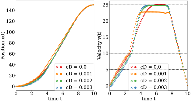
Figure 1: Position $x(t)$ (left) and velocity $v(t)$ (right) of a car with a hysteretic turbo charger and drag force. The turbo mode is also displayed as active (dots) or inactive (crosses).

4.2 Lotka-Volterra fishing with total variation

In this subsection, we present results for a Lotka-Volterra fishing problem with a total variation (TV) and a fixed final time. For two different populations $x_{1}$ and $x_{2}$, which can be interpreted as the biomasses of prey and predator, respectively, binary optimal control is performed. The primary objective is formulated as

$$\min\quad\int_{0}^{T}\|x(t)-x_{r}\|^{2}\mathrm{d}t$$ (9)

for tracking the reference value $x_{r}=\begin{bmatrix}1,1\end{bmatrix}^{\top}$ [23, §5]. The dynamics of the underlying 2-population model can be described by the equations

$$\dot{x}_{1}(t)={} x_{1}(t)-x_{1}(t)x_{2}(t)-c_{1}^{\top}w(t),$$

$$\dot{x}_{2}(t)={} x_{1}(t)x_{2}(t)-x_{2}(t)-c_{2}^{\top}w(t)$$

for given parameters $c_{1},c_{2}\in\mathbb{R}^{5}$ and controls $w(t)\in\{0,1\}^{5}$ [22]. The pointwise constraint $\sum_{i=1}^{5}w_{i}(t)=1$ encodes the choice of one among five fishing options.

To limit the well-known chattering behaviour of the optimal binary controls, we monitor the total variation (in fact, the discrete counterpart thereof)

$$TV(w)\approx\frac{1}{2}\sum_{i=1}^{m}\sum_{k=0}^{N-1}|w_{i,k+1}-w_{i,k}|,$$ (10)

possibly imposing an upper bound $TV(w)\leq U_{TV}$ or including a penalty term $\alpha_{TV}TV(w)$ in the objective [23].

Simulations

The initial state is chosen as $x(0)=\begin{bmatrix}0.5,0.7\end{bmatrix}^{\top}$. The mixed-integer OCP is fully discretized using the explicit Euler scheme over a uniform time grid with final time $T=12$ and $N=30$ intervals. The objective’s integral is approximated by the left Riemann sum. The resulting discretized problem contains $398$ optimization variables (of which $155$ integer-valued) and $31$ nonlinear constraints.

The initial guess values are set to $1$ for all variables. In order to obtain a warm start, the problem (with no TV cost nor limit) is considered with relaxed integrality and solved by Ipopt. Such solution, displayed in Figure 2, is then projected onto $\mathcal{X}$ and used as input $x^{0}$ for Algorithm 3.1 (for all subsequent tests).

Figure 2: Initial guess for the fishing problem, before projection.

We now consider two problems to highlight the effect of penalizing and limiting the TV: with TV cost $\alpha_{TV}=1$, we first solve an instance with no TV upper bound ($U_{TV}=\infty$) and then with $U_{TV}=10$. After executing Algorithm 3.1, its solution is refined with Ipopt by optimizing over real-valued variables. The corresponding results are shown in Figures 3 and 4, respectively. Limiting the (discretized) TV helps to avoid a chattering behaviour of the optimal solution without significantly impairing the tracking performance. Indeed, the solution with the TV constraint appears to improve both components of the objective, namely tracking and switching. This phenomenon indicates that the results in Figure 3 correspond to a suboptimal solution testifying the local nature of Algorithm 3.1.

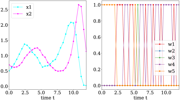
Figure 3: Refined solution for the fishing problem with TV cost $\alpha_{TV}=1$ and no TV limit ($U_{TV}=\infty$).

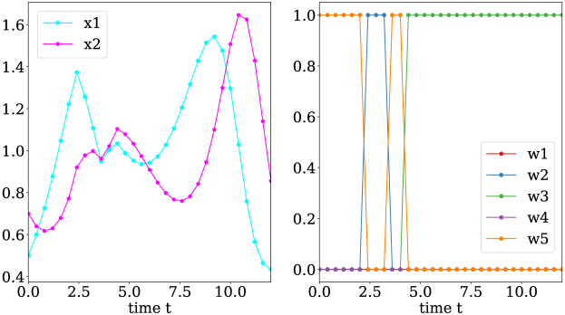
Figure 4: Refined results for a fishing problem with TV cost $\alpha_{TV}=1$ and TV limit $U_{TV}=10$.

As to the numerical performance of Algorithm 3.1, the MIL solver was called 6764 times for the case without TV limit returning a solution after 42 iterations and 150 seconds. For $U_{TV}=10$, these statistics read 2869 MIL calls, 41 iterations and 61 seconds.

4.3 Dynamic facility location problem

Let us now consider a dynamic facility location problem with applications in logistics. Consider a set of $m$ customers and $n$ possible warehouses. Each customer is given by a position $x_{j}\in\mathbb{R}^{2}$ and demand $d_{j}$, $j\in\{1,\ldots,m\}$. Each potential warehouse is associated to a region $R_{i}\subset\mathbb{R}^{2}$, its position $x_{i}$, capacity $u_{i}$, and a binary $b_{i}$ encoding whether it is actually built or not, $i\in\{1,\dots,n\}$. The amount of goods delivered from warehouse $i$ to customer $j$ (to satisfy their demand) is denoted by $l_{ij}$ whose location-dependent transportation cost is denoted by $C_{ij}(x_{i})$. Moreover, building a warehouse $i$ incurs the capacity-dependent construction cost $P_{i}(u_{i})$.

The aim is to determine, which potential warehouses are to be built as well as their position and capacity such that the total cost is minimized:

$$\operatorname*{minimize}~{}\sum_{i=1}^{n}b_{i}\left(P_{i}(u_{i})+\sum_{j=1}^{m}C_{ij}(x_{i})\right)$$ (11)

where $P_{i}$ and $C_{ij}$ are given construction and transportation cost functions, for $i\in\{1,\ldots,n\}$, $j\in\{1,\ldots,m\}$. Several constraints are incorporated into the model. First, urban planning restrictions have to be taken into account: $x_{i}\in R_{i}$ for each warehouse. Next, capacity specifications need to be integrated: $\underline{u}_{i}b_{i}\leq u_{i}\leq\overline{u}_{i}b_{i}$ and $\sum_{j=1}^{m}l_{ij}\leq u_{i}$, with $0\leq\underline{u}_{i}\leq\overline{u}_{i}$ the capacity limits for warehouse $i$. Moreover, customer demands have to be satisfied: $\sum_{i=1}^{n}l_{ij}=d_{j}$ for each customer. Lastly, integrality and nonnegativity conditions are required: $b_{i}\in\{0,1\}$ and $l_{ij}\geq 0$, respectively, for each warehouse $i$ and customer $j$. In order to decouple integer-valued variables and nonlinear functions, these relationships are rewritten by introducing some auxiliary variables and using big-M reformulations.

Simulations

We present results for the problem scenario with $n=30$ regions and $m=10$ customers, depicted in Figure 5, with $1080$ optimization variables (of which $30$ integer-valued) and $330$ nonlinear constraints. Regions $R_{i}$ are placed along two circles and are described by simple bounds for $x_{i}$. Regions are numbered from $1$ to $n$ starting with those at the inner circle and moving counter-clockwise. The capacity bounds are set to $\underline{u}_{i}=10$ and $\overline{u}_{i}=1000$. The construction cost function is chosen as $P_{i}(u):=iu+c_{P}$, $i\in\{1,\ldots,n\}$ where $c_{P}$ is a fixed nonnegative offset. As to the transportation cost function, we consider $C_{ij}(x_{i}):=c_{C}\sqrt{\operatorname{dist}(x_{i},x_{j})}$ where $c_{C}:=(4\sqrt{3\sqrt{2\alpha_{u}}})/3$, $\alpha_{u}=0.1$. Such cost corresponds to the analytical solution for a point-to-point motion (between $x_{i}$ and $x_{j}$) with free final time minimizing both final time and (integral squared) acceleration with cost factors $1$ and $\alpha_{u}$, respectively.

Figure 5 shows a feasible initial guess and the solution obtained for $c_{P}=100$, which selects 7 warehouses that overall strike a good balance between construction and transportation costs. For this instance, Algorithm 3.1 terminated after 42 iterations and 67 seconds calling the MIL solver 936 times.

Finally, we considered instances with increasing values for $c_{P}$. The optimal number of warehouses depending on parameter $c_{P}$ is shown in Figure 6 and, despite some oscillations due to local minima, the overall behaviour is consistent with our expectations in that the number of warehouses decreases with increasing $c_{P}$.

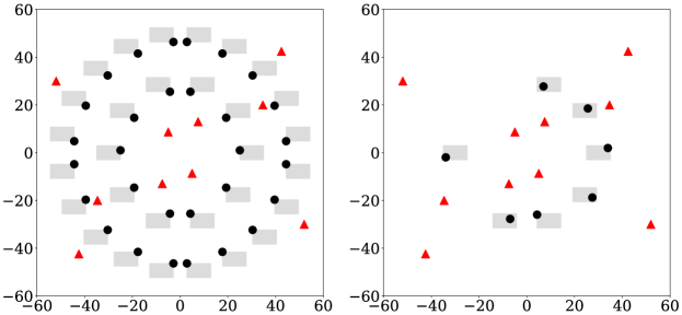
Figure 5: Facility location problem with $n=30$ regions for warehouses (gray rectangles), $m=10$ customers (red triangles), and $c_{P}=100$: position of warehouses actually built (black dots) in initial guess (left) and solution obtained (right).

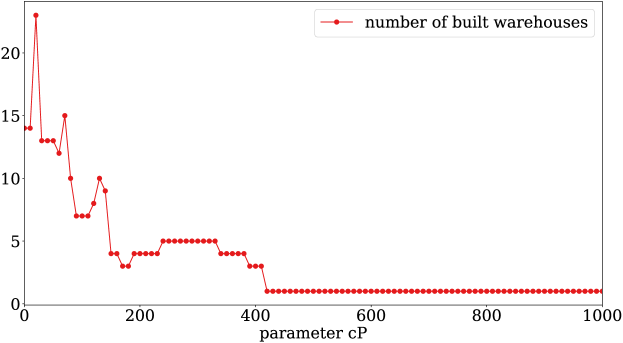
Figure 6: Facility location problem with $n=30$ regions for warehouses and $m=10$ customers: number of warehouses built as a function of $c_{P}$.

5 Conclusions

This work presents an efficient method to address hybrid optimal control problems without any relaxations. The proposed approach is based on the augmented Lagrangian framework and a routine for nonlinear optimization with mixed-integer linear constraints. The robustness and performances of the algorithm were assessed on three problem examples from different fields of application. Promising preliminary results validate the strategy here developed.

Future research should consider the convergence analysis of Algorithm 3.1 and the possibility to integrate other techniques for handling nonlinear constraints.

References

- [1] Pietro Belotti, Christian Kirches, Sven Leyffer, Jeff Linderoth, James Luedtke, and Ashutosh Mahajan. Mixed-integer nonlinear optimization. Acta Numerica, 22:1–131, 2013.
- [2] Ernesto G. Birgin and José M. Martínez. Practical Augmented Lagrangian Methods for Constrained Optimization. Society for Industrial and Applied Mathematics, Philadelphia, PA, 2014.
- [3] Claudia D’Ambrosio, Antonio Frangioni, Leo Liberti, and Andrea Lodi. A storm of feasibility pumps for nonconvex MINLP. Mathematical Programming, 136(2):375–402, 2012.
- [4] Alberto De Marchi. Implicit augmented Lagrangian and generalized optimization. arXiv:2302.00363, 2023.
- [5] Alberto De Marchi. Mixed-integer linearity in nonlinear optimization: a trust region approach. arXiv:2310.17285, 2023.
- [6] Alberto De Marchi, Xiaoxi Jia, Christian Kanzow, and Patrick Mehlitz. Constrained composite optimization and augmented Lagrangian methods. Mathematical Programming, 201(1):863–896, 2023.
- [7] Alberto De Marchi and Patrick Mehlitz. Local properties and augmented Lagrangians in fully nonconvex composite optimization. arXiv:2309.01980, 2023.
- [8] Alberto De Marchi and Andreas Themelis. An interior proximal gradient method for nonconvex optimization. arXiv:2208.00799, 2022.
- [9] Brecht Evens, Puya Latafat, Andreas Themelis, Johan Suykens, and Panagiotis Patrinos. Neural network training as an optimal control problem: An augmented lagrangian approach. In 2021 60th IEEE Conference on Decision and Control (CDC), pages 5136–5143, 2021.
- [10] Oliver Exler, Thomas Lehmann, and Klaus Schittkowski. A comparative study of SQP-type algorithms for nonlinear and nonconvex mixed-integer optimization. Mathematical Programming Computation, 4(4):383–412, 2012.
- [11] Anthony V. Fiacco and Garth P. McCormick. Nonlinear Programming: Sequential Unconstrained Minimization Techniques. Wiley, New York, 1968.
- [12] Matthias Gerdts. A variable time transformation method for mixed-integer optimal control problems. Optimal Control Applications and Methods, 27(3):169–182, 2006.
- [13] Matthias Gerdts. Optimal Control of ODEs and DAEs. De Gruyter Oldenbourg, 2023. 2nd Edition.
- [14] Ignacio E. Grossmann and Francisco Trespalacios. Systematic modeling of discrete-continuous optimization models through generalized disjunctive programming. AIChE Journal, 59(9):3276–3295, 2013.
- [15] Mirko Hahn, Sven Leyffer, and Sebastian Sager. Binary optimal control by trust-region steepest descent. Mathematical Programming, 197(1):147–190, 2023.
- [16] Christian Kirches, Paul Manns, and Stefan Ulbrich. Compactness and convergence rates in the combinatorial integral approximation decomposition. Mathematical Programming, 188(2):569–598, 2021.
- [17] Sven Leyffer and Paul Manns. Sequential linear integer programming for integer optimal control with total variation regularization. ESAIM: COCV, 28:66, 2022.
- [18] Armin Nurkanovic and Moritz Diehl. NOSNOC: A software package for numerical optimal control of nonsmooth systems. IEEE Control Systems Letters, 6:3110–3115, 2022.
- [19] Jan Oldenburg and Wolfgang Marquardt. Disjunctive modeling for optimal control of hybrid systems. Computers & Chemical Engineering, 32(10):2346–2364, 2008.
- [20] Christoph Plate, Sebastian Sager, Martin Stoll, and Manuel Tetschke. Second-order partial outer convexification for switched dynamical systems. IEEE Transactions on Automatic Control, pages 1–13, 2024.
- [21] Rien Quirynen and Stefano Di Cairano. Sequential quadratic programming algorithm for real-time mixed-integer nonlinear MPC. In 2021 60th IEEE Conference on Decision and Control (CDC), pages 993–999. IEEE Press, 2021.
- [22] Sebastian Sager. A benchmark library of mixed-integer optimal control problems. In Jon Lee and Sven Leyffer, editors, Mixed Integer Nonlinear Programming, pages 631–670, 2012. https://mintoc.de/index.php/Lotka_Volterra_absolute_fishing_problem, accessed: 2024-03-06.
- [23] Sebastian Sager, Michael Jung, and Christian Kirches. Combinatorial integral approximation. Mathematical Methods of Operations Research, 73(3):363–380, 2011.
- [24] Pantelis Sopasakis, Emil Fresk, and Panagiotis Patrinos. OpEn: Code generation for embedded nonconvex optimization. IFAC-PapersOnLine, 53(2):6548–6554, 2020. 21st IFAC World Congress.
- [25] Clemens Zeile, Nicolò Robuschi, and Sebastian Sager. Mixed-integer optimal control under minimum dwell time constraints. Mathematical Programming, 188(2):653–694, 2021.