Inverse Garment and Pattern Modeling with a Differentiable Simulator

Abstract

The capability to generate simulation-ready garment models from 3D shapes of clothed humans will significantly enhance the interpretability of captured geometry of real garments, as well as their faithful reproduction in the virtual world. This will have notable impact on fields like shape capture in social VR, and virtual try-on in the fashion industry. To align with the garment modeling process standardized by the fashion industry as well as cloth simulation softwares, it is required to recover 2D patterns. This involves an inverse garment design problem, which is the focus of our work here: Starting with an arbitrary target garment geometry, our system estimates an animatable garment model by automatically adjusting its corresponding 2D template pattern, along with the material parameters of the physics-based simulation (PBS). Built upon a differentiable cloth simulator, the optimization process is directed towards minimizing the deviation of the simulated garment shape from the target geometry. Moreover, our produced patterns meet manufacturing requirements such as left-to-right-symmetry, making them suited for reverse garment fabrication. We validate our approach on examples of different garment types, and show that our method faithfully reproduces both the draped garment shape and the sewing pattern.

1 Introduction

The ability to generate simulation-ready garment twins from 3D shapes of dressed individuals has a wide range of applications in virtual try-on, garment reverse engineering, and social AR/VR. It will allow, from the retrieved garment models, to obtain new animation, or to better capture and interpretate subsequent garment geometry undergoing deformation. This is particularly compelling given the increasing accessibility of detailed 3D scans of individuals in clothing. Such garment recovery system should ideally satisfy the following: high fidelity to faithfully replicate the given 3D geometry, flexible adaptability to obtain new garment simulations on different body shapes and poses, and the ability for the output garment to align with the standard garment modelling process used in both the fashion industry and cloth simulation softwares.

In this paper, we address the challenging problem of estimating animation-ready patterns given a 3D garment on its wearer as input. Our system operates based on a user-selected base pattern mesh and its corresponding 3D sewn garment, whose physically-based draping simulation is computed on the estimated body. Such pattern-based modeling closely mimics the design process for both real-world and synthetic garments, and effectively disentangles the inherent shape from deformations caused by external physical forces and internal fabric properties during simulation. The target sewing pattern is then recovered by iteratively optimizing the simulated garment to fit the target and updating the pattern state through an inverse simulation. Such ability to estimate garment patterns facilitates the adaptation of the reconstructed garment to new conditions for downstream applications. One can synthesize new cloth animations by computing the draping and dynamic simulations of the reconstructed garment on various body shapes or poses. It also enables the users to adjust the size or design of a captured garment. Such competence of convenient garment reanimation and garment retargeting is highly desirable for the aforementioned applications. Our approach does not require a lot of data, and is capable of faithfully replicating intricate garment shape, due to its understanding of physics.

We evaluate our approach on a variety of garment types and demonstrate that our method produces patterns of promising quality. We compare it against the state-of-the-art methods, and report that our method can replicate more detailed deformations and produce more accurate pattern estimations. In summary, we make the following contributions:

• A new formulation of inverse pattern recovery that models the draping garment geometry as a function of the pattern state and physical interaction with the body;

• Enhancing and refining a differentiable simulator to achieve realistic garment reconstruction and precise pattern estimation;

• A new parameterization of the sewing pattern that facilitates the differentiable simulation to achieve the pattern states to best-fit the simulated garment geometry to target geometry;

• A tailored loss function crafted to achieve the pattern, which is compatible with the current garment modeling and fabrication process.

Our generated data and code will be made available for research purposes at https://anonymous.project.website.

2 Related work

2.1 Garment shape recovery from 2D/3D data

Methods reconstructing a single layer mesh for the whole clothed body from one or more 2D images, such as NeRF [57, 59] or PIFu [45] require further 3D segmentation to separate the garment part from the body, which is a challenging problem in itself as addressed by some researchers, either by directly segmenting the input 3D data [2, 44, 53], or by regressing the cloth-to-body displacement map [13, 35]. However, the garment geometries obtained by these works often lack compatibility with existing cloth simulators or trained models for neural simulations due to the missing 2D pattern structure or canonical shapes. Moreover, adapting the geometries to new body shapes poses a significant challenge.

A large body of works exists on video-based 3D reconstruction of body shape and pose [25, 63, 15, 61], or on training deep neural networks to learn garment draping [55, 14, 17, 29] or dynamic garment motion [46, 62, 6, 5, 47] on the body in the light of replacing computation-intensive physics-based simulations. However, with a few exceptions [20, 31, 18], most works concentrate on capturing or reproducing physically plausible deformation of clothes whose canonical shape is known in advance.

Generative models have demonstrated their fitting capacity to given 2D or 3D image inputs. Typically, they solve for optimal parameters in the generative model to obtain a best estimation of the body pose and shape, along with the cloth style. Early models [42, 35, 9] learned the 3D clothing deformation as a displacement function, often conditioned on shape, pose, and style of garment deduced from desired or given target images. Such displacement-based representation assumes one-to-one mapping from the garment vertex to the body, thereby is mostly constrained to tight clothes close to the body in terms of topology and shape, showing reduced expressiveness when it comes to skirt/dress. Alternative representations have been explored, such as implicit surface SMPLicit [16], patch-based surface representation [34], or articulated dense point cloud [36].

Another avenue that has been explored involves reconstructing the target garment through part assembly. Starting from the semantic part detection and parsing of the given depth image, [12] searches in the database of 3D garment parts (skirts, trousers, collars, etc.) and stitches them together to form the final garment. While having the advantage of consistently producing plausible garments, this approach requires an extensive database to deal with the high diversity of garment types and configurations.

Our work is similar in spirit to that of [60], who use search-based optimization to recover both 2D sewing patterns (parameterized by numerical, such as sleeve length, waist width) and the 3D garment such that it minimizes the 2D silhouette difference between the projected 3D garment and the input image. The draped 3D garment shape is obtained by using a physics-based simulator [40]. Unlike theirs, in our work the estimation of pattern parameters are coupled with the physically-based simulation process, allowing for direct and precise mapping of 3D garment error to both the pattern geometry and material parameters.

2.2 Sewing pattern estimation from 3D data

Another related problem is to estimate 2D sewing patterns from 3D garment mesh, a challenge that has been addressed by several methods.

3D-to-2D surface flattening. Several works considered the garment mesh as developable surface and obtained 2D pattern panels by cutting the garment surface into 3D patches and flattening each of them onto a plane. The cutting lines are found either by projecting the predefined seam lines from the body mesh onto the garment mesh [2], along curvature directions expressed in the cross fields [54, 43] on the surface, or through variational surface cutting[49] to minimize the distortion induced by cutting and flattening [58]. While intuitive and versatile, such surface flattening based on a geometric strategy is prone to generating patterns that deviate from traditional panel semantics, or lack of left-to-right symmetry, making them unsuitable for garment production. Moreover, purely geometric methods [2, 43] do not account for the fabric’s elasticity in physical body-cloth interaction during the draping process, often resulting in a sewing pattern that cannot accurately replicate the originally designed garment.

Pattern geometry optimization. [3] invented a fixed point method for direct 3D garment editing and a two-phase optimization approach to get plausible patterns but it may not have an exact solution in the second phase which can meet the goal achieved in the first phase. [56] tries to solve a constrained optimization for adjusting a standard sewing pattern, and the focus is on the garment sizing task (S to XL for instance) which means adjusting a standard sewing pattern for a better fit on another input body shape. The cost function is customized that way so it’s not for generic 3D fitting.

Learning based estimation. The work of [27] explores a learning-based approach for estimating the garment sewing pattern of a given 3D garment shape. Based on a dataset of 3D garments with known sewing patterns covering a variety of garment design, their model is capable of regressing the sewing patterns representing the garment, as well as the stitching information among them. Although it presents an interesting approach, their model has trouble handling conditions beyond the situations represented in the training dataset: The actual dataset used for training limits their model to the drape shapes on average SMPL female body at T-pose, and struggles with garments with different material properties than those used to generate the dataset.

2.3 Differentiable cloth simulator

Our method mainly solves an optimization of parameters coupled with the garment simulation process. We follow the thread of differentiable physics simulation [32, 22, 30, 28, 19] that can optimize parameters to fit the measurement data. To our knowledge, this is the first work that applies the differentiable simulator to recover sewing patterns of garments from the inputs of clothed humans.

3 Method

3.1 Overview

In this section, we describe our method outlined in Fig. 1. Drawing an analogy to garment production, the garment geometry in our work is determined by the style and size of its sewing pattern, which is parameterized for efficient modification (Sect. 3.2). The first component of our system is the linear grading which accounts for capturing the coarse geometry such as size and proportion (Sect. 3.3). The second component further refines the model to capture the detailed garment shape and precise pattern. At the heart of our technique is an optimization-driven pattern refinement based on a differentiable cloth simulator (Sect. 3.4, Sect. 3.5), where the simulated garment is iteratively altered along with the physical parameters.

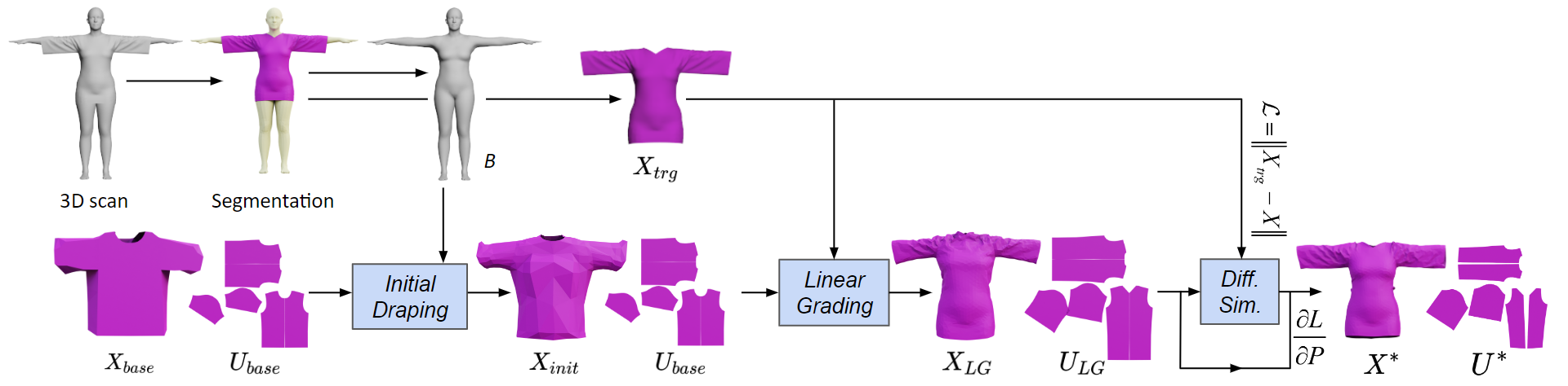
Figure 1: Overview of our method.

3.2 Representation of Base Pattern and Body

The garment shape is determined by the shape and size of its sewing pattern, which is a collection of 2D pieces of textile (panels) that are stitched together and placed around the wearer’s body at the initial stage of the later simulation.

We assume that several base models, i.e., patterns and their corresponding sewn 3D meshes, are available for representative garment categories, which are set by the user depending on the target garment type under consideration. Our system provides three base patterns chosen from the Berkeley Garment Library [40], with the option for users to incorporate their custom-created base models.

Parameterization. The planar pattern mesh $U$ serves as the FEM reference (prior to any deformation) for its corresponding 3D garment mesh $X$ during the later simulation. The mapping between a 2D vertex $u\in U$ to a 3D node $x\in X$ is known from the base models, in the form of a UV Map. A panel is a 2D triangular

mesh bounded by a number of piece-wise curves, each composed of a number of edges. Two curves join at a control point $c^{i}$, which is typically the vertex of curvature discontinuity (corner point), or the vertex having three or more seam-counterparts belonging to other panels (join point) which will be merged into one node at the time of sewing.

The control points are grouped into disjoint sets $\mathcal{C}=\{C_{p}\}$, one for each panel. The points are ordered in a counterclockwise manner within each panel $p$, i.e. $C_{p}=\{c_{p}^{i}\}$. Throughout the pattern optimization process, the control points serve as variables, while the remaining points will be repositioned so as to retain their relative locations with respect to them.

Symmetry detection. To further reduce the dimension of parameter space, and to preserve the left-to-right symmetry (which is often a desirable property in garment production) during optimization, we detect the pattern symmetry in two steps: It first detects inter-panel symmetry by computing for each pair of panels the aligning rigid transformation [48] and evaluating the quality of alignment. If their alignment score is sufficiently high, we remove one of them from the effective control point group ${K}$. Next, we perform intra-panel symmetry detection within ${K}$, by computing for each pair of control points $c_{p}^{i},c_{p}^{j}\in C_{p}$ its axis of symmetry and evaluating the symmetry score for the remainder of control points in $p$. The control points pair with the highest score exceeding a predefined threshold will be used to identify left-to-right symmetry within a panel, which is then used to further reduce control points from ${K}$. The details of the symmetry detection method can be found in the supplementary material.

Sewn garment shape. The sewn 3D garment mesh is made of 2D pattern placed in 3D, topologically stitched along seams, and geometrically deformed to have sufficiently large inter-panel distances in order to avoid any potential body-garment interpenetration. Note that the vertices along the seams will be merged with their seam counterparts on other panel(s) during stitching. Hence, the correspondence between 3D nodes $x\in X$ and 2D vertices $u\in U$ is one-to-many for those on the seams, while it remains one-to-one for the rest.

Body model. The draped shape of a garment is determined by not only the pattern shape $U$, but also the underlying body $B$, and their interaction during contact. We adopt the parametric SMPL model [33] to represent body, for which several efficient registration methods to 3D data exist [7, 8].

3.3 Pattern Linear Grading

In this phase, we aim to perform preliminary geometric deformation at the panel level to approximately capture the target garment by using a number of key measurements in 3D. The main idea is to focus on the open contours (i.e., 3D closed curves composed of edges connected to only one adjacent triangle) extracted from both the target and simulated meshes, and relocate control points so that the corresponding contours are closely aligned in 3D, in terms of circumferences and location along the bone. Note that open contours often carry design features, representing elements like neck lines, hem contours, cuff contours, etc.

Given a base model pair $U_{base}$ and $X_{base}$, an initial draped shape $X_{init}$ is computed on the estimated body $B$, with reference to $U_{base}$. The open contours on both the simulated and the target meshes are extracted, associated with their respective counterparts, the distances between them are measured along the skeleton of the underlying body. The distances, along with the difference in circumference, are used to guide the analytical relocation of control points $\{c^{i}\}$ on the pattern. An algorithmic description is given in the supplementary material.

The above process could potentially lead to substantial location changes of control points, leading to undesirable topological distortion such as fold-over. To preserve the initial topology of the pattern mesh as well as the neighboring relationship among vertices, we employ the 2D deformation method based on Mean Value Coordinates (MVC), similar to [38]. The relative positions of panel boundary vertices are first computed with respect to their neighboring control points, which in turn serve as position constraints for retrieving the remaining interior vertices by means of MVC. The resulting pattern $U_{LG}$ and its corresponding draped garment mesh $X_{LG}$ serve as good initial stage for the subsequent optimization-driven pattern alteration (Sec. 3.5).

3.4 Cloth Simulation

The pattern obtained from the previous phase is only an approximation of the target geometry. In the next phase, we conduct pattern refinements through an optimization tightly coupled with a differentiable cloth simulation. In particular, we extend the differentiable ARCSim [32, 40] by revisiting both the dynamic solve and body-cloth interaction.

3.4.1 Diffenrentible Cloth Simulation

At each forward simulation step, the draping garment over the estimated body is computed, taking into account external and internal forces until an equilibrium is achieved. The implicit Euler integration involves solving a linear system for the cloth motion, which writes as:

$$(M-\Delta t^{2}J)\Delta v=\Delta t(f+vJ\Delta t),$$ (1)

where $f$ is the sum of external forces (gravity, contact force) and internal forces (stretching, bending, etc). $M$ is the block diagonal mass matrix composed of the lumped mass of each node, and $J=\frac{\partial f}{\partial x}$ is the Jacobian of the forces. At each time step $\Delta t$, we solve equation (1) for $\Delta v$ and update the velocity $v$ and position $x$. The equation could be written as $\hat{\mathbf{M}}\mathbf{a}=\hat{\mathbf{f}}$ for simplicity.

After the forward simulation with a predefined number of deltas (10 to 20 in our experiments), a loss $\mathcal{L}$ (Sect. 3.5) is measured between the simulated garment geometry and the target cloth mesh segmented from the 3D input. The error is used to back-propagate gradients to optimize the garment rest shape in terms of pattern parameters. Taking the implicit differentiation from [32], we use the analytical derivatives of the linear solver to compute $\frac{\partial\mathcal{L}}{\partial\hat{\mathbf{M}}}$ and $\frac{\partial\mathcal{L}}{\partial\hat{\mathbf{f}}}$ with the gradients $\frac{\partial\mathcal{L}}{\partial\mathbf{a}}$ backpropagated from $\mathcal{L}$.

3.4.2 Material Model

We employ the linear orthotropic stretching model [50] to quantify the extent of planar internal forces in response to cloth deformation. The model defines the relation between stress $\sigma$ and strain $\epsilon$ using a constant stiffness matrix $\boldsymbol{H}$: $\sigma=\boldsymbol{H}\epsilon$, where

$$\boldsymbol{H} =\left[\begin{array}[]{lll}H_{00}&H_{01}&0\\ H_{01}&H_{11}&0\\ 0&0&H_{22}\end{array}\right],$$ (2)

The bending forces are modeled with piecewise dihedral angles which describes how much the out-of-plane forces would be when subject to cloth bending, as used in [11]:

$$\mathbf{f}_{i}=k\frac{\|\mathbf{e}\|^{2}}{\left\|\mathbf{A}_{1}\right\|+\left\|\mathbf{A}_{2}\right\|}\sin\left(\frac{\pi-\theta}{2}\right)\mathbf{u}_{i},$$ (3)

where $\mathbf{e}$ is the edge vector, $\mathbf{f}_{i}$ is the bending force applied on the $i$-th vertex ($i$=1,…,4), $\mathbf{A}_{1}$ and $\mathbf{A}_{2}$ are the areas of two triangles, $\mathbf{u}_{i}$ is the direction vector of the $i$-th node, and $k$ is the bending stiffness coefficient.

3.4.3 Acceleration of Force Vector Assembly

ARCSim [40, 32] uses the traditional approach of directly solving the linear system after the assembly of the extended mass matrix $\hat{\mathbf{M}}$ and the force vector $\hat{\mathbf{f}}$. The internal forces exerted by a triangle element to its nodes are split and accumulated to the global force vector, where the contributions from multiple adjacent elements are summed up for each node. Such force vector assembly process incurs a considerable overhead cost, as the number of time steps grows. It’s even more expensive for extended mass matrix assembly as it contains the Jacobian of forces, which is large and sparse. We propose an efficient method for accelerating the assembly. As the same assembly is executed for each time integration, we exploit the fact that the inherent topological structure remains unchanged during the simulation, with a sequence of triangle elements in a fixed filling order. We encode this information in a form of a static mapping matrix which maps the batched elementary forces/jacobians to the global force vector/jacobian matrix. This mapping converts the assembly process to a matrix multiplication as depicted in Fig. 2, which is parallelized on a GPU. Additionally, the matrix remains very sparse regardless of the mesh resolution, for which multiple numerical tools are available. It is highly backpropagation-friendly, which boosts the speed (Table 1). More details on this scheme are in the supplementary material.

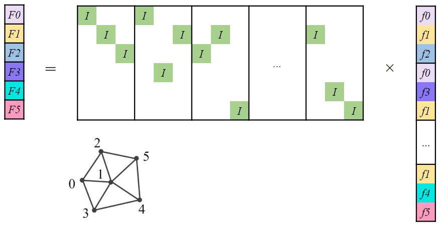
Figure 2: The per-node force vector assembly by merging partial contributions is encoded in the form of a static matrix, which is sparse.

3.4.4 Efficient Body Cloth Interaction

One important component for draping simulation lies in the body-garment interaction, which involves the contact force computation and the garment-body collision handling, for which many algorithms have been proposed [11, 52, 21], In particular, the one based on non-rigid impact zones [21] has been made differentiable by Liang et al [32]. However, it remains computationally expensive, leading to rapid growth of the computation graph (i.e. memory-hungry) during forward simulation, and struggles to accommodate high-resolution meshes. Hence, we chose to compromise by implementing a learning-based collision handling scheme that makes use of the signed distance function (SDF). Specifically, we have adopted a variant of DeepSDF [39] with MLPs with periodic activation functions [51] which learns the body surface more precisely than the vanilla DeepSDF [41]. We integrate our trained SDF-net into the simulation process to replace the collision handling in differentiable ARCSim, significantly enhancing the speed of both forward and reverse simulation while maintaining the performance level.

When the predicted signed distance of a query garment vertex $x$ falls below a threshold (indicating close proximity to the body), the repulsion force is triggered between the body and the garment, with its magnitude inversely proportional to their distance. Frictional force is also elicited when there is relative movement along the surface tangent. While the repulsion forces prevents the interpenetration, occasional collisions might still occur and need correction after the dynamic simulation. To this end, for any garment vertex $x$ with negative signed distance, we present the collision resolving setup, correcting the interpenetration by:

$$\tilde{x}=x+(\delta-sdf(x))\times n$$ (4)

if $sdf(x)<0$, where $n=\frac{\nabla sdf(x)}{\left|\nabla sdf{x}\right|}$ is the spatial gradient of $sdf(\cdot)$ (also the surface normal), and $\delta$ denotes the collision thickness. To our knowledge, our work is the first to integrate SDF-based collision handling into a differentiable simulation process, where SDFs are leveraged not only for collision response but also for repulsion and friction force computation.

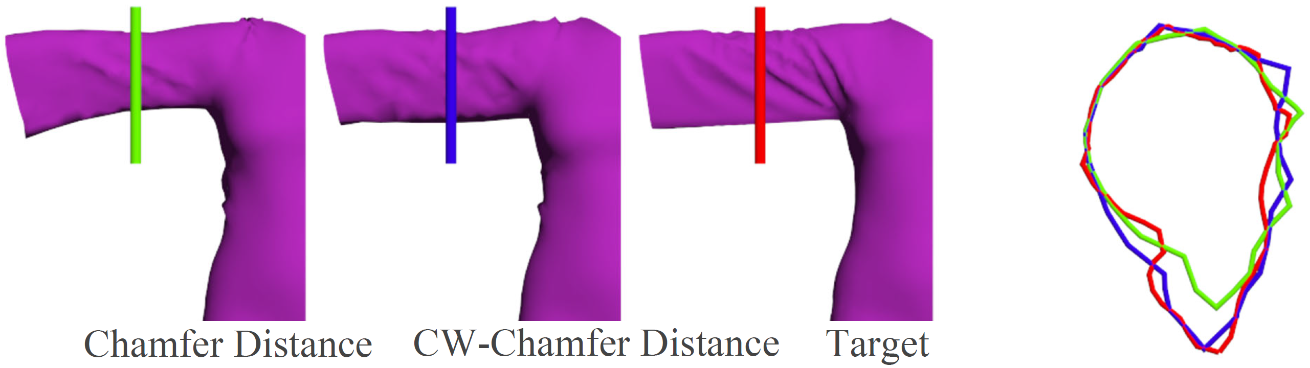
Figure 3: The cross-sectional curves on the right, generated from three meshes on the left: two simulated meshes, and the target. The colors of the cutting planes are used to draw the cross-sections. The curvature-weighted Chamfer (blue) leads to a sleeve draping silhouette closer to the ground truth (red), compared to the standard Chamfer distance (green).

3.5 Optimization-based Pattern Alteration

In this phase, we further refine both the pattern state $U_{LG}$ and the simulated garment $X_{LG}$ obtained from the previous stage through optimization using the differentiable draping simulator. At each iteration, the simulated garment geometry $X=\{x_{i}\}$ is compared with the target $T=\{t_{i}\}$ using a loss function, subsequently utilized by a gradient-based algorithm to refine the pattern shape. We define the following loss over the effective control points $K$ and the physical parameters $\Gamma$:

$$\mathcal{L}=\mathcal{L}_{rec}(X=\textit{Sim}(U(K),\Gamma;\textit{SMPL}(\theta,\beta)),T)+\lambda_{seam}\mathcal{L}_{seam}(U(K)),$$ (5)

where $\lambda$’s are weights. It combines the reconstruction loss $\mathcal{L}_{rec}$ and the seam-consistency loss $\mathcal{L}_{seam}$ penalizing the inconsistent curve lengths along the seam. The reconstruction error is composed of the Chamfer distances $\mathcal{L}_{CF}$ measured both between the surfaces ($X$ and $T$) and among open contours ($X_{open}$ and $T_{open}$),

$$\mathcal{L}_{rec}=\mathcal{L}_{CF}(X,T)+\lambda_{open}\mathcal{L}_{CF}(X_{open},T_{open})+\lambda_{mat}\mathcal{L}_{mat}(\Gamma).$$ (6)

The Chamfer distance, widely used for fitting deformable surfaces, has proven to work well in most cases. However, we observed that it is not sufficient for certain garment targets, due to its “myopia” that each point only considers its nearest neighbor on the other mesh, neglecting the surroundings. In regions with high curvatures, often present in the folded geometry of loose clothes, this can lead to lower geometric accuracy (See Fig. 3). Hence, we use curvature-weighted Chamfer distance [10] instead, which prioritizes high-curvature regions, subsequently improving the reconstruction of densely folded regions:

$$\mathcal{L}_{CWCF}\left(X,T\right)=\frac{1}{\left|X\right|}\sum_{\mathbf{x}\in X}\kappa(\tilde{\mathbf{t}})\min_{\mathbf{t}\in T}\|\mathbf{x}-\mathbf{t}\|^{2}+\frac{1}{\left|T\right|}\sum_{\mathbf{t}\in T}\kappa(\mathbf{t})\min_{\mathbf{x}\in X}\|\mathbf{t}-\mathbf{x}\|^{2},$$ (7)

with $\kappa$ the mean curvature and $\tilde{\mathbf{t}}=\arg\min_{\mathbf{y}\in T}{(\mathbf{x}-\mathbf{y})}$. The seam loss serves as the regularization that guarantees the consistent curve lengths of two panels along the seam:

$$L_{seam}(U)=\sum_{i}^{|S|}\sum_{j}^{|E_{i}|=|{E_{i}^{corr}}|}\left(|e_{i}^{j}|-|e_{i}^{corr,j}|\right)^{2},$$ (8)

where $\mathcal{S}=\{\mathcal{S}_{i}\}\subset X$ denotes the set of 3D seam curves, and $E_{i},E_{i}^{corr}\subset U$ are the sets of edges $e^{j}=u^{j}-u^{j+1}$ along the 2D panel curves comprising the seam counterparts of $\mathcal{S}_{i}$.

We also optimize over the physical parameters $\boldsymbol{H}$ and $k$ by adding them into the variable set:

$$\Gamma:=(H_{00},H_{01},H_{11},H_{22},k).$$ (9)

To penalize unrealistic material parameter combinations, we constrained the elements within the physically plausible ranges (above a non-negative threshold 1e-6). These physical parameters are added to the variable set in later iterations, once the pattern shapes reach an approximate optimum.

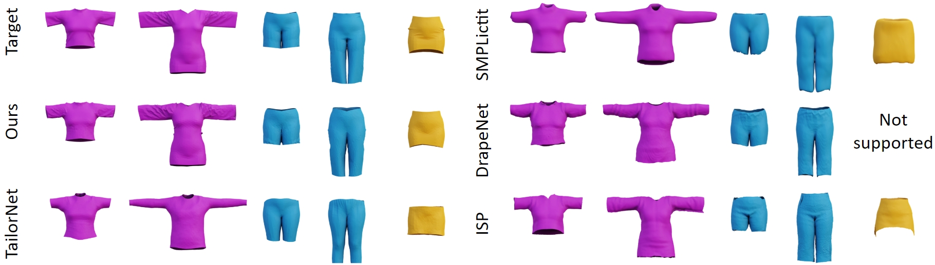
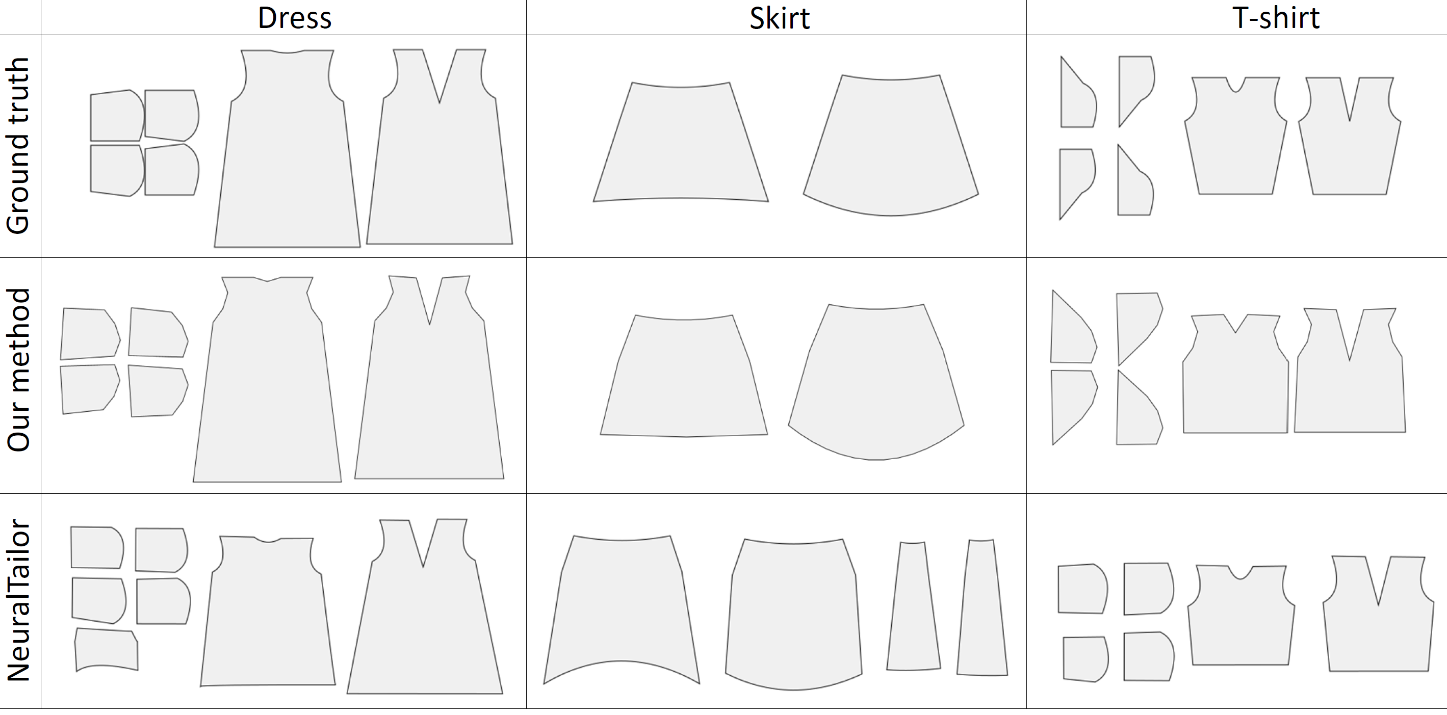
Figure 4: Up: Comparison of 3D garment reconstruction of our method with others [42, 16, 17, 29]. Our method reproduces faithful garment shapes, even accounting for intricate geometry details like wrinkles on large sleeves. Down: 2D pattern estimation from 3D garment meshes. From top to bottom: The ground truth, our results, and the results from NeuralTailor[27]. Best viewed on screen zoomed-in.

4 Experiments

4.1 Implementation details

We now describe the main implementation details. Further information is provided in the supplementary material.

Simulation. We set one time step $\Delta t$ to 0.05s, and the number of time steps for one forward simulation between 10 and 20. The garment resolution tested ranges from 1K to 3K vertices. By vectorizing as much as possible the force and jacobian computation, our extension to ARCSim differentiable cloth simulator [32] allows to run all its computations on a GPU. Table 1 summarizes the computation time of linear solve for the baseline model [32] and ours measured on a NVIDIA GeForce 3090, for T-shirt garments with different resolutions (1K to 3K). Note that in our model the first iteration involves the construction of the deterministic mapping, which is reused for the subsequent iterations. On the contrary, the overhead of assembly is required for every iterations in the baseline model. We compared our SDF query network with classical KDTree-based SDF, and the evaluation times were 0.108s and 0.0054s, respectively, for 3K query points. The periodic activations used significantly reduce the average prediction error of SDF values (from 1.19mm to 0.2mm), similarly to the results of [51]. Overall, we observed 15 times speedup compared to [32].

Table 1: The computational time recorded of matrix assembly and linear solve(in seconds) using the baseline model and ours, measured on a T-shirt garment with varying resolutions. Note how our method improves the speed as the number of iterations increases, especially during the reverse process.

	Baseline[32]		Ours
	1	20	1	20	speedup
1K (forward)	2.8	83.7	19.1	59.4	1.4x
1K (reverse)	7.0	155.6	2.7	60.0	2.59x
2K (forward)	8.4	178.1	67.6	133.0	1.34x
2K (reverse)	17.2	466.0	6.3	128.7	3.62x
3K (forward)	12.3	257.9	133.6	228.6	1.13x
3K (reverse)	24.7	505.4	12.0	186.3	2.71x

Optimization. The variables are optimized by using the Adam optimizer [24], with a learning rate $10^{-3}$, $\beta_{1}$ = 0.9, $\beta_{2}$ = 0.999. We empirically set $\lambda_{open}=0.1$, $\lambda_{mat}=0.01$ and $\lambda_{seam}=0.01$. We observed that the addition of material parameters noticeably impacts the result. Conversely, excluding these parameters from optimization might lead to distorted panels. We present the results of a related ablation study in the supplementary material. The material parameters are initialized with a specific set from the material library that spans a range of fabrics, from which the user selects the most probable one. Note that the pattern variables are effectively initialized through the linear grading.

4.2 Quantitative and Qualitative Comparisons

We evaluate our model on a number of representative garment types and compare it with previous works. We first evaluate the performance on 3D garment reconstruction, then on 2D pattern estimation. To carry out a fair comparison, we use the garment meshes of a third-party dataset [26] as targets (i.e. test data), which is an unseen dataset for all evaluated methods. It is also one of the rare datasets that provide 2D sewing patterns for every 3D garment mesh, enabling the evaluation of our results in both 3D reconstruction and 2D pattern estimation. We describe the detailed results below.

3D garment reconstruction. We compare our approach to the related methods for garment fitting, and utilize 3D garment geometry as targets. We run the Adam optimizer [24] for a varying number of iterations until the convergence for each method, while noting that the parameter space representing the garment geometry differs among them: The coordinates of effective control points and material parameters for our method, the $\gamma$ garment style parameter for TailorNet [42], the latent vector $z=[z_{cut},z_{style}]$ describing garment cut and style for SMPLicit [16], and the latent codes $z$’s encoding the garment characteristics in DrapeNet and ISP[17, 29]. The results are quantitatively evaluated using two metrics: Chamfer distance to the ground truth mesh points, and the angular error to measure the similarity of the computed normal vectors , similar to [4]. As shown in Table 2, our method is consistently better than others , which is confirmed by quanlitative results, shown in Fig. 4. We observe that the performance of the data-driven approaches is biased by the training dataset. It is clear that TailorNet basically has learned over tight-fit datasets, so it does not generalize very well when fitting to loose styles, as seen in the Pants example. In contrast, our approach reconstructs accurate 3D geometry, for both loose and tight garments.

Table 2: Quantitative evaluation in 3D (garment reconstruction) and 2D (pattern estimation). To measure the accuracy of 2D patterns, we evaluate the turning function metric for comparing polygonal shapes [1] and the surface error (the average of normalized surface difference error computed for each patch).

	3D Reconstruction					2D Estimation
	Chamfer distance / Normal similarity					Turning /Surface area
Garments	SMPLicit	TailorNet	Drapenet	ISP	Ours	NeuralTailor	Ours
T-shirt	1.4 /-	0.331 / 0.081	0.689 / 0.129	0.297 / 0.094	0.112 / 0.049	10.70 / 0.13	9.53 / 0.09
Dress	3.2 / -	1.305 / 0.161	0.619 / 0.135	0.189 / 0.131	0.110 / 0.075	11.3 / 0.37	10.96 / 0.10
Shorts	1.3 / -	1.036 / 0.050	0.131 / 0.048	0.202 / 0.095	0.126 / 0.043	7.61 / 0.05	7.37 / 0.04
Pants	2.9 / -	2.587 / 0.104	0.485 / 0.085	0.185 / 0.077	0.142 / 0.049	6.89 / 0.01	7.12 / 0.08
Skirt	6.5 / -	1.30 / 0.063	- / -	0.435 / 0.093	0.106 / 0.014	4.54 / 1.11	3.99 / 0.04

2D Pattern Estimation. The quantity of research focusing on sewing pattern recovery directly from a given 3D input data is rather limited, with majority of them dedicated to precise but minor adjustments to existing patterns [56, 3]. We compare our work with NeuralTailor [27], a deep learning framework that predicts a structural representation of a sewing pattern from a 3D garment shape. To be able to compare with the ground-truth patterns, the experiments were conducted under favorable conditions for their work – We selected five patterns from their proper dataset as the ground-truth ones. This means that NeuralTailor might have seen these data during training. Then, we generate 3D drape shapes by using an independent simulator [37] differing from both ours and theirs. Some of the results are illustrated in Fig. 4, while additional results can be found in the supplementary material. We observe that their method makes very good predictions on the trouser-like garments as the geometric variation of pants and shorts are limited and well covered in the their training dataset. For the other garment types, however, our method produces better results. To quantitatively measure the quality of estimated 2D patterns, we have used two metrics: (1) the turning function metric for comparing polygonal shapes [1], and (2) the relative error in surface area, as determined by averaging normalized surface difference error $\frac{1}{\left|P\right|}\sum\frac{\Delta A(P_{i})}{A(P_{i})}$ computed for each panel $P_{i}$.

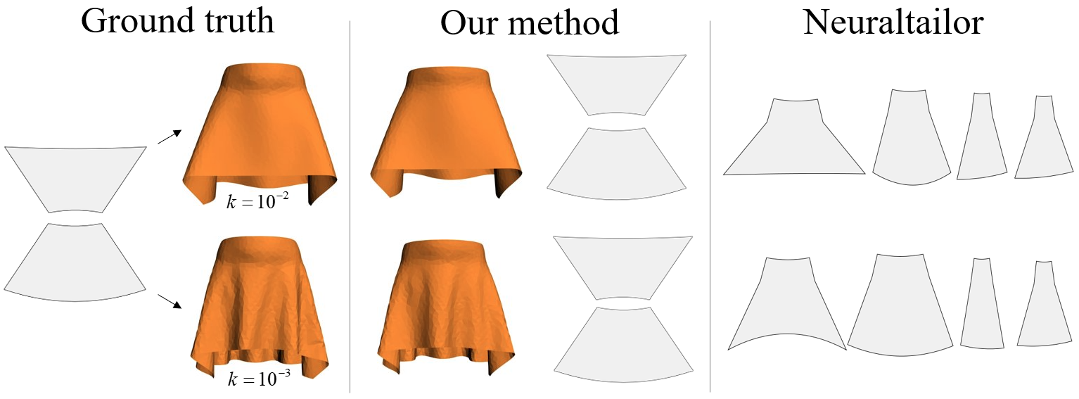
Figure 5: Sewing patterns estimated from two input meshes, both simulated from an identical ground-truth pattern but with varying bending coefficients. By optimization over bending coefficient, our method correctly finds the panel shapes, compared to the alternative method.

4.3 Recovery of Physical Parameters

To demonstrate the capability of our method to faithfully recover physics, two draping skirt meshes were simulated using identical sewing patterns but varying only the physical parameters. Then we used them as targets and compared our estimated patterns with those generated from NeuralTailor. As shown in Fig. 5, our method can faithfully capture 3D garment geometric variations originating from different bending parameters, while producing consistent patterns close to the ground truth. On the contrary, NeuralTailor translates the geometric variation into that of panels, yielding a significantly different pattern for each target instance.

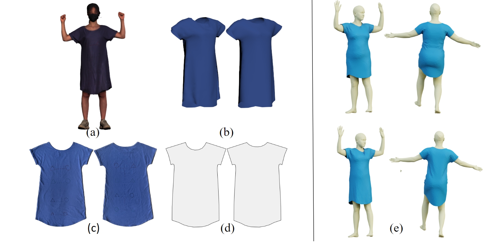
Figure 6: Results of our method evaluated using 3D scan data. (a) Input 3D scan; (b) Segmented target (left) and simulated garment (right); (c) Ground-truth pattern; (d) Estimated pattern; (e) Retargeted garment to two new SMPL bodies.

4.4 Evaluation on 3D Scan Data and Retargeting

We conducted a qualitative evaluation of our method using a 3D body scan. As shown in Fig. 6, it outputs reasonable, quality estimations of the 3D garment and the 2D pattern. We also showcase an example of how our recovered garment can be retargeted to new conditions. As the recovered pattern is simulation compatible, it can be easily reused by a simulator to generate new draping shapes. The dress model recovered from the 3D scan has been successfully used to produce compelling results on novel body poses and shapes.

5 Conclusion

We have presented a method to recover simulation-ready garment models from a given 3D geometry of a dressed person. Basing our work on a differentiable simulator, we retrieve the 2D sewing pattern through inverse simulation, ensuring that the physically based draping of the corresponding sewn garment closely matches the given target. Our experimental results confirm that our system can produce simulation- and fabrication-ready patterns on a range of representative garment geometries, outperforming comparable state-of-the-art methods. These improvements collectively render the use of differentiable simulation practical in terms of both time efficiency and memory usage. Combining our model with a learning-based method would be an interesting future investigation.

Appendix 0.A Base patterns

Our system provides base models selected and modified from the Berkeley Garment Library [40] (Sect. 3.2 in our paper), which users can modify as needed. Additionally, users have the option to import their own personalized or customized base models into the system. Fig. 7 shows three base models (t-shirt/dress, pants, and skirt) used in our experiments.

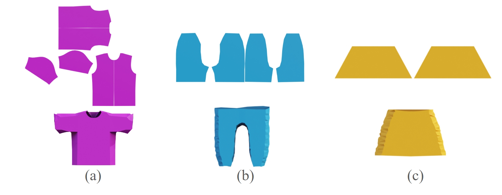
Figure 7: The base models for three garment topologies. (a) t-shirt/dress; (b) pants; and(c) skirt.

Appendix 0.B Matrix assembly acceleration

Similar to the force vector $\hat{\mathbf{f}}$, the matrix $\hat{\mathbf{M}}$ in Sect. 3.4 of our paper is constructed by aggregating the local contributions from individual elements into the corresponding locations.  Each triangle element (element hereafter) yields nine Jacobians, each representing a partial derivative of the force with respect to the position of a node ($\frac{\partial f_{i}}{\partial x_{j}}$), $i,j$=1,2,3. The Jacobians for all elements are packed into a Jacobian stack as illustrated in Fig. 8 (d), where we use $mn$ to denote $\frac{\partial f_{m}}{\partial x_{n}}$ ($m$, $n$: global indices) for a compact representation. In ARCSim [32, 40], these Jacobians are assembled to $\hat{\mathbf{M}}$ through a total of $F\times 3\times 3$ assignment or addition operations, where $F$ represents the number of triangles in the garment mesh. Optimizing this process becomes crucial, especially considering its higher computational cost compared to the force vector assembly (The optimization of the latter has been discussed in Sect. 3.4 of the main paper).

To this end, we propose to realize the Jacobian assembly using matrix multiplication. $\hat{\mathbf{M}}$ is a sparse matrix, and moreover, directly representing the mapping from the Jacobian stack to the matrix form is not feasible, although it would be ideal for leveraging GPU-accelerated matrix multiplication. We address this issue by introducing an intermediate data structure called compressed Jacobian vector (Fig. 8(a)). It is a set of Jacobians for each force-node combination, which is obtained by first reshaping the Jacobian stack into a Jacobian vector (Fig. 8(c)), and by encoding the mapping from the per-element Jacobian to the compressed Jacobian vector as a static mapping matrix (Fig. 8(b)). Then a GPU-based sparse matrix multiplication is performed, effectively substituting the iteration-based Jacobian assembly. This results in a considerable acceleration of the assembly process as reported in Table. 1 of our paper.

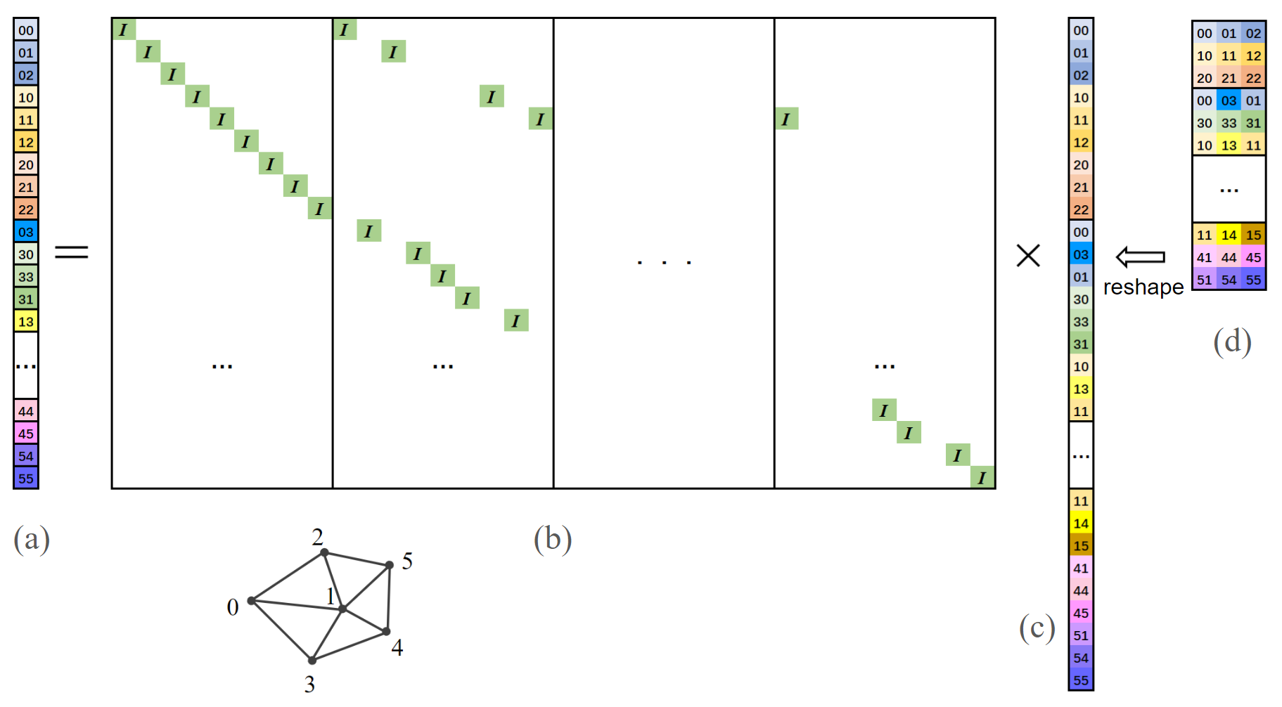
Figure 8: The assembly of a compressed Jacobian vector is obtained by a static matrix multiplication, encoding the mapping from the per-element Jacobian (d) to the per force-node Jacobian (a).

Finally, the Jacobians in the compressed vector are transferred to $\hat{\mathbf{M}}$ (Fig.9). Note that the number of operations reduces to $N+2\times E$ ($N$: number of nodes, $E$: number of edges), compared to the original $F\times 3\times 3$.

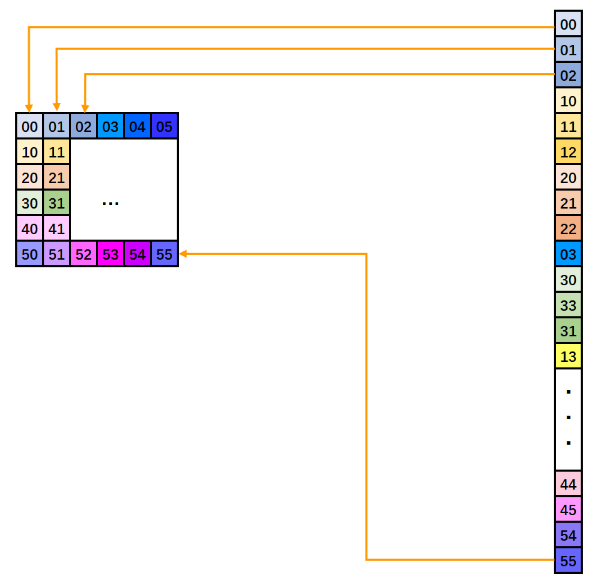
Figure 9: Transferring compressed Jacobians to the extended mass matrix $\hat{\mathbf{M}}$.

Appendix 0.C Ablation study

Here we report the results of our ablation study, where we examine the contributions of individual components to the overall performance (Table 3). Our baseline model achieved a Chamfer distance precision (CF) of 0.1103 (in mm) and a reduced cosine distance of normals (NOR) of 0.075. It outperforms other settings where the curvature-weighted Chamfer loss is replaced with the vanilla Chamfer (CF: 0.115, NOR:0.085), when the seam consistency loss term is removed (CF:0.117, NOR:0.076), or when the optimization of physical parameters was disabled (CF: 0.113, NOR: 0.081). These results confirm the importance of both loss terms and the integration of physical properties in the optimization process.

Fig. 10 illustrates the reconstructed models obtained from the ablation study. We observe that our model (Fig. 10(e)) bears the closest visual resemblance to the target. The use of weighted Chamfer distance allows for better capture of the armpit region and the lower part of the sleeve (Fig. 10(b)). The absence of seam loss leads to a puckered seam around the shoulder, resulting from the extra tension exerted on the the shorter seam (Fig. 10(c)). The optimization of physical parameters helps to recover fine wrinkles, as well as more plausible pattern estimation. As we can see in Fig. 10(d), the “A-line” shape of the body/dress has been solely attributed to the increasing panel width along the torso, when the material parameters were disregarded during the optimization.

Table 3: Ablation Study.

Method	Chamfer distance (CF)	Normal difference (NOR)
Ours(w/o curvature CF)	0.115	0.085
Ours(w/o seam loss)	0.117	0.076
Ours(w/o physics)	0.113	0.081
Ours	0.110	0.075

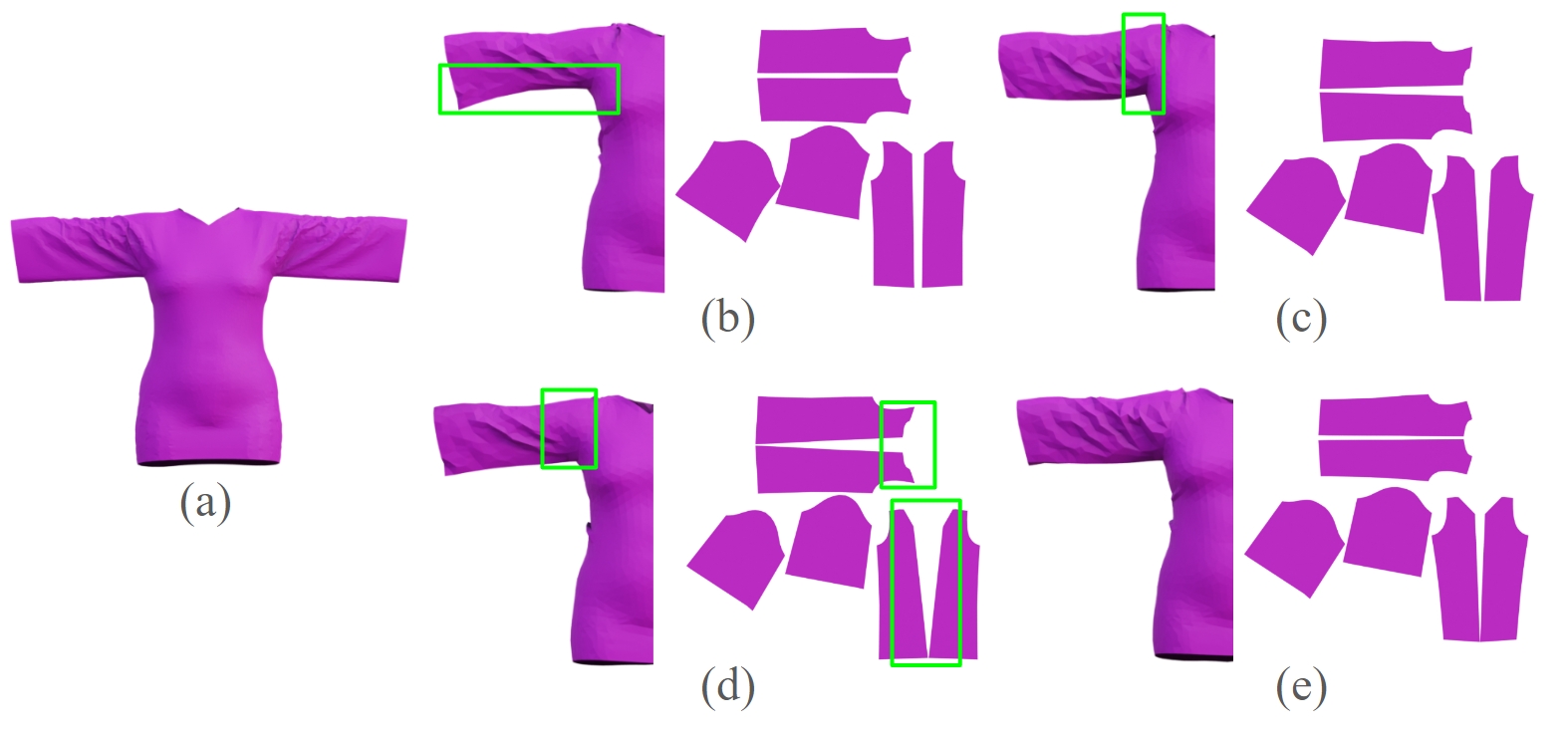
Figure 10: Results of our ablation study on loss terms. (a) Target; (b) Chamfer loss without curvature weights (i.e. vanilla Chamfer); (c) without seam loss; (d) without physical parameters; (e) Ours.

Appendix 0.D Pattern symmetry detection

A detailed algorithmic description of inter-panel and intra-panel symmetry detection can be found in Algorithm 1.

Appendix 0.E Linear grading

Once the initial draping of the 3D base garment has been simulated, the 2D pattern is adjusted to minimize the difference in both circumferences and axial distances along the bone between corresponding open contours in 3D. Contours around the hip or waist, cuff contours on the arm, are typically used in this linear grading step. In Fig. 11, the distance between the target cuff $O_{t}$ and the source $O_{s}$ measured along the arm bones, together with the difference in their circumferences, determines the amount of the displacement $|\overrightarrow{\vec{d}}|$ of control points on the corresponding open curve (in blue) of the pattern. In the 2D panel, the direction of $\overrightarrow{\vec{d}}$ is derived by computing and normalizing the midpoint of the two control points on the open curve minus the average of the remaining control points, while the width-changing vectors are computed by subtracting each control point from the other and normalizing it. Readers can refer to Algorithm 2 for a detailed procedure on pairing and computing axial distances for open contours.

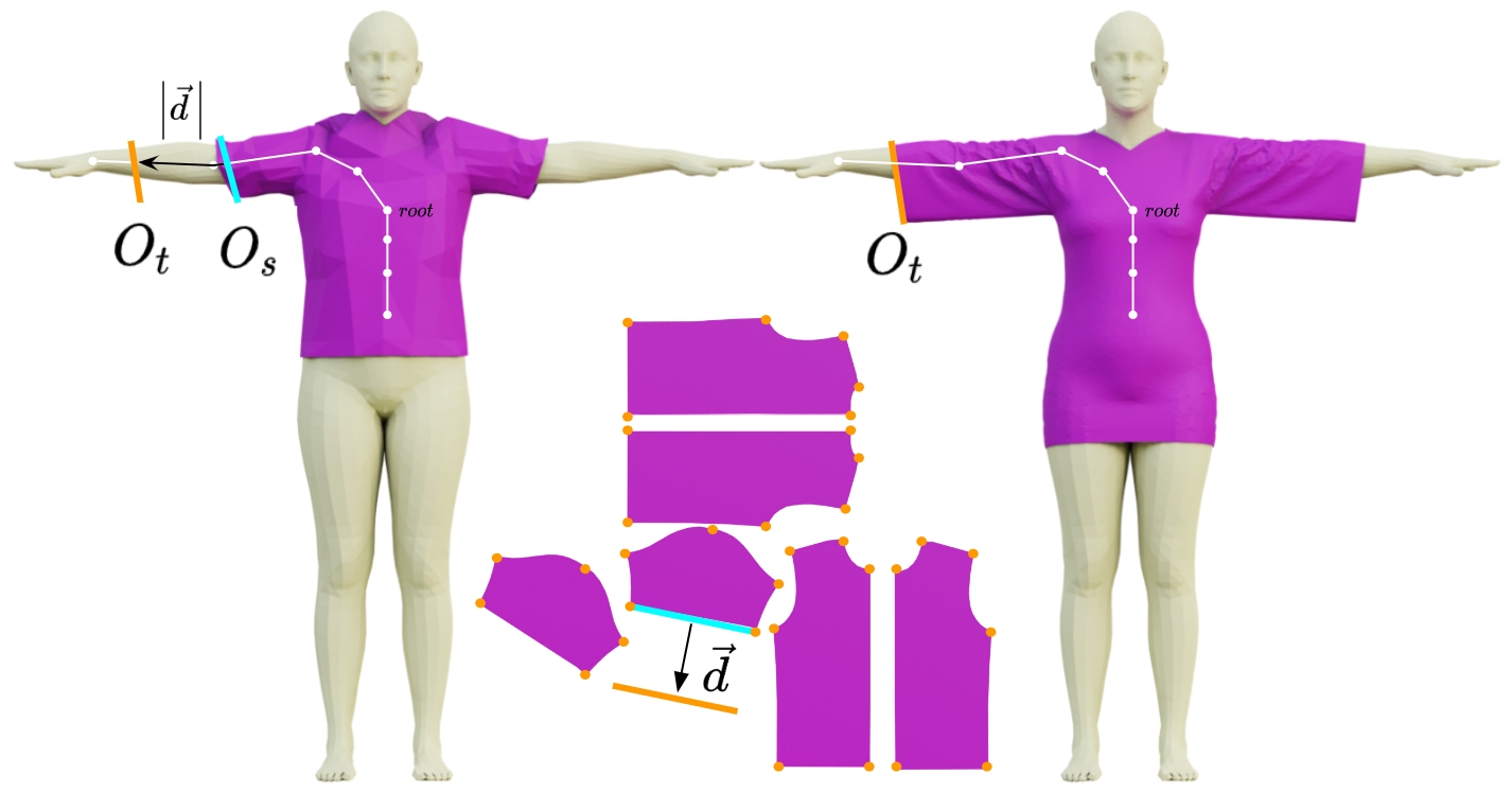
Figure 11: An example of linear grading. The axial distance $\overrightarrow{\vec{d}}$ between open contours from the source mesh (left) to the target mesh (right) is used to displace the corresponding open curve (in blue) in the 2D panel.

Appendix 0.F Limitations

Our approach presents several limitations that suggest avenues for future exploration. First, the iterative optimization process involving forward and reverse simulation is time-consuming. Further acceleration can be employed to achieve faster convergence in optimization processes [23]. Second, although our linear grading scheme effectively adjusts the base model to align with the target prior to the optimization, our final results can be sensitive to initial values, potentially resulting in different local minima, as well as to predefined design choices such as mesh resolution and the identification of control points on the panels. Combining our model with a learning-based method to achieve good initialization would be an interesting future investigation.

Input:
$C$ ={$C_{p}$}, where $C_{p}$ is an ordered set of control points of panel $p$.

Output:
$K$: Effective control points

$InterSym$: A set of panel pairs in correspondence and the orthogonal matrix {($C_{p}$, $C_{p^{\prime}}$, $M_{p}$)}, so that $c_{p}^{i}\in C_{p}$ corresponds to $c_{p\textquoteright}^{i}\in C_{p^{\prime}}$ and $(C_{p}\times M)\simeq C_{p^{\prime}}$.

$IntraSym$: A set of control point pairs in mirror symmetry and the reflection matrix per panel {$(Q,Q^{\prime},M)_{p}$} such that $(Q\times M)\simeq Q^{\prime}$.

Algorithm 1 Pattern symmetry detection.

SymmetryDetection($C$)

$K$, $InterSym$ $\leftarrow$ InterSymmetry($C$)

$IntraSym$ $\leftarrow$ $\emptyset$

for each $C_{p}\in K$ do

     1. ($U$, $U^{\prime}$, $matrix$) $\leftarrow$ IntraSymmetry($C_{p}$)

     2. $IntraSym$ $\cup$ ($U$, $U^{\prime}$, $M$)

     3. $K\leftarrow K\setminus U^{\prime}$

end for

$K,InterSym,IntraSym$

InterSymmetry($C$)

$K$ $\leftarrow$ $C$, $InterSym$ $\leftarrow$ $\emptyset$

for $C_{p}$ in $K$ do

     $error_{p}\leftarrow\infty$, $M_{p}\leftarrow I$, $p^{\prime}\leftarrow-1$

     for $C_{q}$ in $K$ do

         1. $C_{q}^{r}$ $\leftarrow$ ReversePointsOrder($C_{q}$)

         2. $error_{tmp},M_{tmp},C_{tmp}$ $\leftarrow$ RigidAlignment($C_{p},C_{q}^{r}$)

         if  $error_{tmp}<\epsilon$ and $error_{tmp}<error_{p}$ then

              $p^{\prime}$ $\leftarrow$ $q$, $error_{p}\leftarrow error_{tmp}$, $M_{p}\leftarrow M_{tmp}$, $C_{p}$ $\leftarrow$ $C_{tmp}$

         end if

     end for

     if  $p^{\prime}\neq-1$ then

         1. $InterSym$ $\cup$ ($C_{p}$,$C_{p^{\prime}}$,$M_{p}$)

         2. $K\leftarrow K\setminus C_{p^{\prime}}$

     end if

end for

$K,InterSym$

IntraSymmetry($C_{p}$)

$l$ $\leftarrow$ $\left|C_{p}\right|$

for  $i=0...l/2$ do

     $U$ $\leftarrow$ $\left\{c_{p}^{u}\right\}$, $u=\left\{i...i+\left\lfloor l/2\right\rfloor-1\right\}$

     $V$ $\leftarrow$$\left\{c_{p}^{v}\right\}$, $v=\left\{(i+\left\lceil l/2\right\rceil)\%l...(i+l-1)\%l\right\}$

     $V^{r}$ $\leftarrow$ ReversePointsOrder($V$)

     $error$, $M$, $U^{\prime}$ $\leftarrow$ RigidAlignment($U,V^{r}$)

     if  $error$ $<$ $\epsilon$ then

         return ($U$,$U^{\prime}$,$M$)

     end if

end for

RigidAlignment($C_{1},C_{2}$)

$l$ $\leftarrow$ $\left|C_{2}\right|$, $error_{min}$ $\leftarrow$ $\infty$, $M^{*}$ $\leftarrow I$ , $C_{2}^{*}\leftarrow C_{2}$

for $i=0...l$ do

     $C_{2}$ $\leftarrow$ Concatenate($C_{2}[i:],C_{2}[0:i]$)

     $error$, $matrix$ $\leftarrow$ OrthogonalProcrustes($C_{1},C_{2}$)

     if $error<error_{min}$ then

         $M^{*}$ $\leftarrow$ $matrix$, $C_{2}^{*}\leftarrow C_{2}$, $error_{min}$ $\leftarrow$ $error$

     end if

end for

$error_{min},M^{*},C_{2}^{*}$

Input:
$\left\{B_{k}\right\}$: Bone vectors from SMPL joints

$\left\{O^{s}\right\}$: Open contours on a source mesh $S$

$\left\{O^{t}\right\}$: Open contours on a target mesh $T$

Output:
$\left\{O^{s},O^{t},d_{st}\right\}$: A set of open contour pairs ($O^{s}\in S$, $O^{t}\in T$) and their distance along the skeleton

Algorithm 2 Axial distance computation among open contours.

MeasureDistanceAlongBones($\left\{B_{k}\right\}$, $\left\{O^{s}\right\}$, $\left\{O^{t}\right\}$)

for each $O^{s}$ do

     $\left\{L_{i}^{s}\right\}\leftarrow$EncircledBones $(O^{s},\left\{B_{k}\right\})$

end for

for each $O^{t}$ do

     $\left\{L_{j}^{t}\right\}\leftarrow$ EncircledBones $(O^{t},\left\{B_{k}\right\})$

end for

$MAP\leftarrow\emptyset$

for each $(O^{s},O^{t})$ pair do

     $MAP^{st}\leftarrow\emptyset$

     for each $(L_{i}^{s},L_{j}^{t})$ pair do

         if bodypartname($B_{i}^{s}$) == bodypartname($B_{j}^{t})$ then    //bodyparts: torso and four limbs

              $MAP^{st}\leftarrow MAP^{st}\cup\{(O^{s},O^{t},L_{i}^{s},L_{j}^{t})\}$

         end if

     end for

     $MAP\leftarrow MAP\cup\left\{MAP^{st}\right\}$

end for

for each $MAP^{st}$ in $MAP$ do

     1. take $\left\{(L_{i}^{s},L_{j}^{t})\right\}$ from $MAP^{st}$

     2. $i^{*}\leftarrow\mathop{\arg\min}_{i}\|h_{i}^{s}\in L_{i}^{s}\|$

     3. take $P_{i^{*}}^{s},P_{j^{*}}^{t}$ from $(L_{i^{*}}^{s},L_{j^{*}}^{t})$

     4. $d(O^{s},O^{t})\leftarrow distToRoot(P_{j^{*}}^{t})-distToRoot(P_{i^{*}}^{s})$

end for

$\left\{O^{s},O^{t},d_{st}=d(O^{s},O^{t})\right\}$

EncircledBones($O,\left\{B_{k}\right\}$)

Input:

$\left\{B_{k}\right\}$: bone vectors from SMPL joints

$O$: open contour on a mesh

Output:

$L=\{L_{i}\},L_{i}=\{(B_{i},u_{i},P_{i},h_{i})\}$ where bone vector $B_{i}$ is enclosed by $O$, and $u_{i}$ and $h_{i}$ are the axial and the perpendicular distances of the contour center in relation to $B_{i}$.

$L\leftarrow\emptyset,O_{center}\leftarrow center(O)$

for each $B_{i}$ in $\left\{B_{k}\right\}$ do

     1. $J_{i}^{parent},J_{i}^{child}\leftarrow\text{Two joints of bone vector }B_{i}$

     2. $u_{i}\leftarrow\frac{\overrightarrow{J_{i}^{parent}J_{i}^{child}}\cdot\overrightarrow{J_{i}^{parent}O_{center}}}{\|\overrightarrow{J_{i}^{parent}J_{i}^{child}}\|^{2}}$       // axial distance from the parent

     3. $P_{i}\leftarrow J_{i}^{parent}+u*(\overrightarrow{J_{i}^{parent}J_{i}^{child}}))$ // projection of $O_{center}$ onto the bone

     4. $h_{i}\leftarrow\|O_{center}-P_{i}\|$                           // distance to the bone

     if $0<u_{i}<1$  then

         $L_{i}\leftarrow\left\{B_{i},u_{i},P_{i},h_{i}\right\}$

         $L\cup L_{i}$

     end if

end for

$L=\left\{L_{i}\right\}$

References

- [1] Arkin, E., Chew, L., Huttenlocher, D., Kedem, K., Mitchell, J.: An efficiently computable metric for comparing polygonal shapes. IEEE Transactions on Pattern Analysis and Machine Intelligence 13(3), 209–216 (1991). https://doi.org/10.1109/34.75509
- [2] Bang, S., Korosteleva, M., Lee, S.H.: Estimating garment patterns from static scan data. In: Computer Graphics Forum. vol. 40, pp. 273–287. Wiley Online Library (2021)
- [3] Bartle, A., Sheffer, A., Kim, V.G., Kaufman, D.M., Vining, N., Berthouzoz, F.: Physics-driven pattern adjustment for direct 3d garment editing. ACM Trans. Graph. 35(4), 50–1 (2016)
- [4] Bednarik, J., Parashar, S., Gundogdu, E., Salzmann, M., Fua, P.: Shape reconstruction by learning differentiable surface representations. In: Proceedings of the IEEE/CVF Conference on Computer Vision and Pattern Recognition. pp. 4716–4725 (2020)
- [5] Bertiche, H., Madadi, M., Escalera, S.: Pbns: physically based neural simulator for unsupervised garment pose space deformation. arXiv preprint arXiv:2012.11310 (2020)
- [6] Bertiche, H., Madadi, M., Escalera, S.: Neural cloth simulation. ACM Trans. Graph. 41(6) (nov 2022). https://doi.org/10.1145/3550454.3555491
- [7] Bhatnagar, B.L., Sminchisescu, C., Theobalt, C., Pons-Moll, G.: Combining implicit function learning and parametric models for 3d human reconstruction. In: European Conference on Computer Vision (ECCV). Springer (aug 2020)
- [8] Bhatnagar, B.L., Sminchisescu, C., Theobalt, C., Pons-Moll, G.: Loopreg: Self-supervised learning of implicit surface correspondences, pose and shape for 3d human mesh registration. In: Advances in Neural Information Processing Systems (NeurIPS) (December 2020)
- [9] Bhatnagar, B.L., Tiwari, G., Theobalt, C., Pons-Moll, G.: Multi-garment net: Learning to dress 3d people from images. In: Proceedings of the IEEE/CVF international conference on computer vision. pp. 5420–5430 (2019)
- [10] Bongratz, F., Rickmann, A.M., Pölsterl, S., Wachinger, C.: Vox2cortex: fast explicit reconstruction of cortical surfaces from 3d mri scans with geometric deep neural networks. In: Proceedings of the IEEE/CVF Conference on Computer Vision and Pattern Recognition. pp. 20773–20783 (2022)
- [11] Bridson, R., Marino, S., Fedkiw, R.: Simulation of clothing with folds and wrinkles. In: ACM SIGGRAPH 2005 Courses, pp. 3–es (2005)
- [12] Chen, X., Zhou, B., Lu, F., Wang, L., Bi, L., Tan, P.: Garment modeling with a depth camera. ACM Transactions on Graphics (TOG) 34(6), 1–12 (2015)
- [13] Chen, X., Pang, A., Yang, W., Wang, P., Xu, L., Yu, J.: Tightcap: 3d human shape capture with clothing tightness field. ACM Trans. Graph. 41(1) (nov 2021). https://doi.org/10.1145/3478518
- [14] Chen, X., Wang, G., Zhu, D., Liang, X., Torr, P., Lin, L.: Structure-preserving 3d garment modeling with neural sewing machines. Advances in Neural Information Processing Systems 35, 15147–15159 (2022)
- [15] Choi, H., Moon, G., Chang, J.Y., Lee, K.M.: Beyond static features for temporally consistent 3d human pose and shape from a video. In: Proceedings of the IEEE/CVF conference on computer vision and pattern recognition. pp. 1964–1973 (2021)
- [16] Corona, E., Pumarola, A., Alenyà, G., Pons-Moll, G., Moreno-Noguer, F.: Smplicit: Topology-aware generative model for clothed people. In: CVPR (2021)
- [17] De Luigi, L., Li, R., Guillard, B., Salzmann, M., Fua, P.: Drapenet: Garment generation and self-supervised draping. In: Proceedings of the IEEE/CVF Conference on Computer Vision and Pattern Recognition. pp. 1451–1460 (2023)
- [18] Feng, Y., Yang, J., Pollefeys, M., Black, M.J., Bolkart, T.: Capturing and animation of body and clothing from monocular video (2022)
- [19] Guo, J., Li, J., Narain, R., Park, H.: Inverse simulation: Reconstructing dynamic geometry of clothed humans via optimal control. In: 2021 IEEE/CVF Conference on Computer Vision and Pattern Recognition (CVPR). pp. 14693–14702. IEEE Computer Society, Los Alamitos, CA, USA (jun 2021). https://doi.org/10.1109/CVPR46437.2021.01446
- [20] Habermann, M., Xu, W., Zollhoefer, M., Pons-Moll, G., Theobalt, C.: Deepcap: Monocular human performance capture using weak supervision. In: IEEE Conference on Computer Vision and Pattern Recognition (CVPR). IEEE (jun 2020)
- [21] Harmon, D., Vouga, E., Tamstorf, R., Grinspun, E.: Robust treatment of simultaneous collisions. In: ACM SIGGRAPH 2008 papers, pp. 1–4 (2008)
- [22] Hu, Y., Liu, J., Spielberg, A., Tenenbaum, J.B., Freeman, W.T., Wu, J., Rus, D., Matusik, W.: Chainqueen: A real-time differentiable physical simulator for soft robotics. In: 2019 International conference on robotics and automation (ICRA). pp. 6265–6271. IEEE (2019)
- [23] Jang, J., Yun, W.H., Kim, W.H., Yoon, Y., Kim, J., Lee, J., Han, B.: Learning to boost training by periodic nowcasting near future weights. In: Krause, A., Brunskill, E., Cho, K., Engelhardt, B., Sabato, S., Scarlett, J. (eds.) Proceedings of the 40th International Conference on Machine Learning. Proceedings of Machine Learning Research, vol. 202, pp. 14730–14757. PMLR (23–29 Jul 2023)
- [24] Kingma, D.P., Ba, J.: Adam: A method for stochastic optimization. In: International Conference on Learning Representations (ICLR) (2015), http://arxiv.org/abs/1412.6980
- [25] Kocabas, M., Athanasiou, N., Black, M.J.: Vibe: Video inference for human body pose and shape estimation. In: Proceedings of the IEEE/CVF conference on computer vision and pattern recognition. pp. 5253–5263 (2020)
- [26] Korosteleva, M., Lee, S.H.: Generating datasets of 3d garments with sewing patterns. In: Vanschoren, J., Yeung, S. (eds.) Proceedings of the Neural Information Processing Systems Track on Datasets and Benchmarks. vol. 1 (2021)
- [27] Korosteleva, M., Lee, S.H.: Neuraltailor: reconstructing sewing pattern structures from 3d point clouds of garments. ACM Transactions on Graphics (TOG) 41(4), 1–16 (2022)
- [28] Larionov, E., Eckert, M.L., Wolff, K., Stuyck, T.: Estimating cloth elasticity parameters using position-based simulation of compliant constrained dynamics. arXiv preprint arXiv:2212.08790 (2022)
- [29] Li, R., Guillard, B., Fua, P.: Isp: Multi-layered garment draping with implicit sewing patterns. Advances in Neural Information Processing Systems 36 (2024)
- [30] Li, Y., Du, T., Wu, K., Xu, J., Matusik, W.: Diffcloth: Differentiable cloth simulation with dry frictional contact. ACM Transactions on Graphics (TOG) 42(1), 1–20 (2022)
- [31] Li, Y., Habermann, M., Thomaszewski, B., Coros, S., Beeler, T., Theobalt, C.: Deep physics-aware inference of cloth deformation for monocular human performance capture (2021)
- [32] Liang, J., Lin, M., Koltun, V.: Differentiable cloth simulation for inverse problems. Advances in Neural Information Processing Systems 32 (2019)
- [33] Loper, M., Mahmood, N., Romero, J., Pons-Moll, G., Black, M.J.: Smpl: A skinned multi-person linear model. ACM transactions on graphics (TOG) 34(6), 1–16 (2015)
- [34] Ma, Q., Saito, S., Yang, J., Tang, S., Black, M.J.: Scale: Modeling clothed humans with a surface codec of articulated local elements. In: Proceedings of the IEEE/CVF Conference on Computer Vision and Pattern Recognition. pp. 16082–16093 (2021)
- [35] Ma, Q., Yang, J., Ranjan, A., Pujades, S., Pons-Moll, G., Tang, S., Black, M.J.: Learning to dress 3d people in generative clothing. In: Proceedings of the IEEE/CVF Conference on Computer Vision and Pattern Recognition. pp. 6469–6478 (2020)
- [36] Ma, Q., Yang, J., Tang, S., Black, M.J.: The power of points for modeling humans in clothing. In: Proceedings of the IEEE/CVF International Conference on Computer Vision (ICCV). pp. 10974–10984 (Oct 2021)
- [37] 3ds Max: Autodesk. https://www.autodesk.com/products/3ds-max/
- [38] Meng, Y., Mok, P.Y., Jin, X.: Computer aided clothing pattern design with 3d editing and pattern alteration. Computer-Aided Design 44(8), 721–734 (2012)
- [39] Mu, J., Qiu, W., Kortylewski, A., Yuille, A.L., Vasconcelos, N., Wang, X.: A-sdf: Learning disentangled signed distance functions for articulated shape representation. 2021 IEEE/CVF International Conference on Computer Vision (ICCV) pp. 12981–12991 (2021), https://api.semanticscholar.org/CorpusID:233240742
- [40] Narain, R., Samii, A., O’brien, J.F.: Adaptive anisotropic remeshing for cloth simulation. ACM transactions on graphics (TOG) 31(6), 1–10 (2012)
- [41] Park, J.J., Florence, P., Straub, J., Newcombe, R., Lovegrove, S.: Deepsdf: Learning continuous signed distance functions for shape representation. In: Proceedings of the IEEE/CVF conference on computer vision and pattern recognition. pp. 165–174 (2019)
- [42] Patel, C., Liao, Z., Pons-Moll, G.: Tailornet: Predicting clothing in 3d as a function of human pose, shape and garment style. In: IEEE Conference on Computer Vision and Pattern Recognition (CVPR). IEEE (jun 2020)
- [43] Pietroni, N., Dumery, C., Falque, R., Liu, M., Vidal-Calleja, T., Sorkine-Hornung, O.: Computational pattern making from 3d garment models. ACM Transactions on Graphics (TOG) 41(4), 1–14 (2022)
- [44] Pons-Moll, G., Pujades, S., Hu, S., Black, M.J.: Clothcap: Seamless 4d clothing capture and retargeting. ACM Transactions on Graphics (ToG) 36(4), 1–15 (2017)
- [45] Saito, S., , Huang, Z., Natsume, R., Morishima, S., Kanazawa, A., Li, H.: Pifu: Pixel-aligned implicit function for high-resolution clothed human digitization. arXiv preprint arXiv:1905.05172 (2019)
- [46] Santesteban, I., Otaduy, M.A., Casas, D.: Learning-based animation of clothing for virtual try-on. Computer Graphics Forum 38(2), 355–366 (2019). https://doi.org/10.1111/cgf.13643
- [47] Santesteban, I., Otaduy, M.A., Casas, D.: Snug: Self-supervised neural dynamic garments. In: Proceedings of the IEEE/CVF Conference on Computer Vision and Pattern Recognition. pp. 8140–8150 (2022)
- [48] Schönemann, P.H.: A generalized solution of the orthogonal procrustes problem. Psychometrika 31(1), 1–10 (1966)
- [49] Sharp, N., Crane, K.: Variational surface cutting. ACM Transactions on Graphics (TOG) 37(4), 1–13 (2018)
- [50] Sifakis, E., Barbič, J.: Fem simulation of 3d deformable solids: a practitioner’s guide to theory, discretization and model reduction. In: Acm siggraph 2012 courses, pp. 1–50 (2012)
- [51] Sitzmann, V., Martel, J., Bergman, A., Lindell, D., Wetzstein, G.: Implicit neural representations with periodic activation functions. Advances in Neural Information Processing Systems 33, 7462–7473 (2020)
- [52] Tang, M., Manocha, D., Tong, R.: Fast continuous collision detection using deforming non-penetration filters. In: Proceedings of the 2010 ACM SIGGRAPH symposium on Interactive 3D Graphics and Games. pp. 7–13 (2010)
- [53] Tiwari, G., Bhatnagar, B.L., Tung, T., Pons-Moll, G.: Sizer: A dataset and model for parsing 3d clothing and learning size sensitive 3d clothing. In: Computer Vision–ECCV 2020: 16th European Conference, Glasgow, UK, August 23–28, 2020, Proceedings, Part III 16. pp. 1–18. Springer (2020)
- [54] Vaxman, A., Campen, M., Diamanti, O., Panozzo, D., Bommes, D., Hildebrandt, K., Ben-Chen, M.: Directional field synthesis, design, and processing. In: Computer graphics forum. vol. 35, pp. 545–572. Wiley Online Library (2016)
- [55] Vidaurre, R., Santesteban, I., Garces, E., Casas, D.: Fully convolutional graph neural networks for parametric virtual try-on. In: Computer Graphics Forum. vol. 39, pp. 145–156. Wiley Online Library (2020)
- [56] Wang, H.: Rule-free sewing pattern adjustment with precision and efficiency. ACM Transactions on Graphics (TOG) 37(4), 1–13 (2018)
- [57] Wang, Z., Wu, S., Xie, W., Chen, M., Prisacariu, V.A.: Nerf–: Neural radiance fields without known camera parameters. arXiv preprint arXiv:2102.07064 (2021)
- [58] Wolff, K., Herholz, P., Ziegler, V., Link, F., Brügel, N., Sorkine-Hornung, O.: 3d custom fit garment design with body movement. arXiv preprint arXiv:2102.05462 pp. 1–12 (2021)
- [59] Xu, H., Alldieck, T., Sminchisescu, C.: H-nerf: Neural radiance fields for rendering and temporal reconstruction of humans in motion. In: Ranzato, M., Beygelzimer, A., Dauphin, Y., Liang, P., Vaughan, J.W. (eds.) Advances in Neural Information Processing Systems. vol. 34, pp. 14955–14966. Curran Associates, Inc. (2021)
- [60] Yang, S., Pan, Z., Amert, T., Wang, K., Yu, L., Berg, T., Lin, M.C.: Physics-inspired garment recovery from a single-view image. ACM Trans. Graph. 37(5) (nov 2018). https://doi.org/10.1145/3026479
- [61] Zhang, J., Tu, Z., Yang, J., Chen, Y., Yuan, J.: Mixste: Seq2seq mixed spatio-temporal encoder for 3d human pose estimation in video. In: Proceedings of the IEEE/CVF conference on computer vision and pattern recognition. pp. 13232–13242 (2022)
- [62] Zhang, M., Ceylan, D., Mitra, N.J.: Motion guided deep dynamic 3d garments. ACM Trans. Graph. 41(6) (nov 2022). https://doi.org/10.1145/3550454.3555485
- [63] Zheng, C., Zhu, S., Mendieta, M., Yang, T., Chen, C., Ding, Z.: 3d human pose estimation with spatial and temporal transformers. In: Proceedings of the IEEE/CVF International Conference on Computer Vision. pp. 11656–11665 (2021)
Input: