Design and Performance Comparison of FuzzyPID and Non-linear Model Predictive Controller for 4-Wheel Omni-drive Robot

Abstract

Trajectory tracking for an Omni-drive robot presents a challenging task that demands an efficient controller design. To address the limitations of manual tuning, we introduce a self-optimizing controller named fuzzyPID, leveraging the analysis of responses from various dynamic and static systems. The rule-based controller design is implemented using Matlab/Simulink, and trajectory tracking simulations are conducted within the CoppeliaSim environment. Similarly, a non-linear model predictive controller(NMPC) is proposed to compare tracking performance with fuzzyPID. We also assess the impact of tunable parameters of NMPC on its tracking accuracy. Simulation results validate the precision and effectiveness of NMPC over fuzzyPID controller while trading computational complexity.

1 Introduction

In recent years, the Omni-directional mobile robot has garnered attention and interest from various research communities due to its unique drive mode, robust maneuver control, and diverse applications across different fields. In comparison to various driving techniques, Omni-based robots offer controlled motion in all directions, allowing them to track user-defined paths or optimal trajectories with low computation costs [1, 2].

The development of an optimal path for a robot to navigate in both static and dynamic environments has been a persistent concern for researchers. Several path-generating algorithms, such as Grassfire, Dijkstra, $A^{*}$, and RRT, have been extensively used in mobile robotics to provide optimal solutions [3]. Among these algorithms, $A^{*}$ is commonly employed for 2D plane navigation, utilizing a heuristic approach to generate the desired trajectory. However, the paths generated by $A^{*}$ often consist of straight segments and sharp angular turns, which may be undesirable for navigating robots. To address this, path-smoothing techniques are applied to soften breakpoints and enhance parametric continuity [4].

Conventional PID controllers have been widely employed in mobile robotics for efficient speed control [5] and waypoint tracking [6]. However, optimizing these controllers for desirable output characteristics can be challenging, and they may not be suitable for a wide range of operating conditions [5, 7]. Consequently, an alternative and effective approach to controller design is utilizing fuzzy logic. Fuzzy logic controllers leverage sets of rules derived from the responses of various static and dynamic systems to adjust tuning parameters based on fuzzy input variables [8, 9]. These controllers exhibit good system performance, transient response, and disturbance rejection capabilities. Moreover, they have been successfully applied to various non-linear plants that are challenging to model due to a lack of sufficient parameters [10, 11]. From a driving perspective, studies such as [12, 13] have successfully evaluated the performance of path planners designed based on fuzzy logic for Omni-drive robots.

With the advancement of powerful computing devices, optimization-based control techniques have become integral in various autonomous mobile industries [14]. Model Predictive Control (MPC) is one such method widely used for path tracking of mobile robots, as it takes into consideration various constraints for optimal control inputs [15, 16, 17, 18, 19]. In comparison with traditional PID methods, MPC offers higher accuracy, smoother control inputs, and increased resistance to external disturbances. Papers such as [20, 16] also highlight the superior performance of MPC over PID controllers, especially when considering kinematic constraints in mobile robots. Considering this, different variants of MPC-based path tracking controllers have been evaluated in recent years, based on the nature of the prediction model’s nonlinearity and the representation of output state quantities [21, 22]. In 2007, the paper by Conceiccao et al. [23] proposed non-linear MPC based on error kinematics models for Omni-drive robots for path following, which was particularly challenging due to hardware constraints at that time. To address these challenges, linear MPC was introduced, which linearized the robot model to simplify computation operations. In a subsequent paper by Wang et al. [24], the authors designed linear MPC and demonstrated its effectiveness for point stabilization and trajectory tracking. Similarly, Kanjanawanishkul et al. [17] presented and applied linear error MPC in real-time for Omni-drive robots, considering system and input constraints to trade for stability. Furthermore, Grüne et al. [25] introduced various extensions of NMPC for time-varying references with or without terminal constraints.

We utilize CoppeliaSim as the simulation platform to conduct our experiments. We design the physical model of a four-wheel omni-drive robot in SolidWorks and import the URDF format into CoppeliaSim. Subsequently, it is interfaced with Matlab/Simulink via an external API to enable control. Physical parameters such as frictional force and air resistance are maintained at default values in the simulation environment.

In summary, our paper comprises three main sections. The initial two sections are dedicated to modeling the kinematics of the robot and subsequently addressing path planning. Following this, we introduce an Omni-drive controller, employing two distinct methods: fuzzy logic with the Mamdani model and Non-linear Model Predictive Control (NMPC). We proceed to assess and compare the performance of these approaches in guiding the robot along the reference trajectory generated by the path planning algorithms. The design of the Omni-drive controller involves formulating a non-linear predictive model, treated as a cost minimization problem. The objective is to determine optimal control inputs that adhere to bounded input constraints, subsequently applied to the robot kinematics. This ensures the robot effectively follows the desired path outlined by the path planning algorithms.

2 Kinematics model

To derive the kinematics model of an Omni-drive robot, it is essential to be aware of the geometric configuration of each wheel with respect to the robot’s Center of Gravity (COG). This knowledge is crucial for understanding how the global velocity of the robot is distributed to each wheel, assuming the absence of roller skidding. The kinematics model establishes the relationship between wheel angular velocity and the robot’s global velocity, and vice versa. In this context, the global coordinate are aligned with the local coordinate frame of the robot. We extend the approach taken by [26] to derive the kinematic of 4-wheel Omni-drive robot.

The global velocity of robot is written as ($\dot{x}$, $\dot{y}$, $\dot{\theta}$) and angular velocity of each wheel is denoted by ($\dot{\phi}_{1}$, $\dot{\phi}_{2}$, $\dot{\phi}_{3}$, $\dot{\phi}_{4}$) which are at an angle of $\dfrac{\pi}{4}$, $\dfrac{3\pi}{4}$, $\dfrac{5\pi}{4}$, $\dfrac{7\pi}{4}$ respectively. Robot body radius and wheel radius are also taken as $R$ and $r$. Then the translation velocity of each wheel hub $v_{i}$ can be formed as the combination of pure translation and pure rotational part of robot [26]. Thus, Fig. 2 shows each wheel has a velocity equal to the expression given as,

$$v_{i}=-\sin(\theta+\alpha_{i})\dot{x}+\cos(\theta+\alpha_{i})\dot{y}+R\dot{\theta}$$ (1)

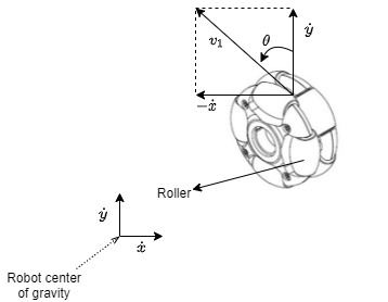
Figure 1: Component division of translational velocity of omni wheel

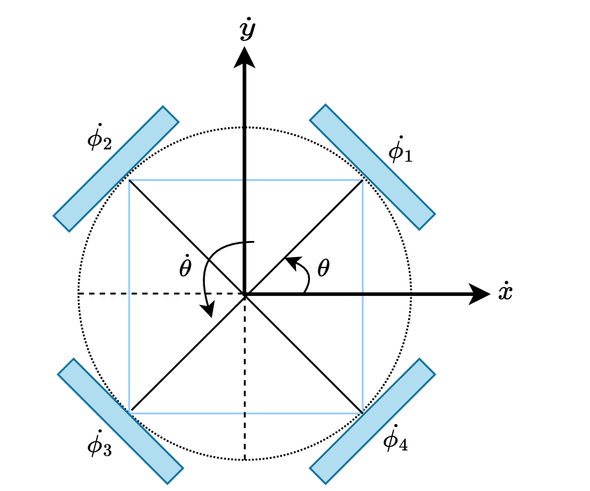
Figure 2: Kinematic diagram of four-wheel omni robot

where, $\theta$ + $\alpha_{i}$ is the offset angle of each wheel w.r.t COG. $\theta$ is $\dfrac{\pi}{4}$ in case of a four-wheel omni robot as shown in Fig. 2 and $\alpha_{i}$ is $\dfrac{\pi}{2}(i-1)$ for the wheel i=1,…,4 respectively. Now, the kinematics model of the robot can be represented in matrix form using equation (1) as,

$$\begin{bmatrix}\dot{\phi}_{1}\\ \dot{\phi}_{2}\\ \dot{\phi}_{3}\\ \dot{\phi}_{4}\end{bmatrix}=\frac{1}{r}\begin{bmatrix}-\sin(\theta+\alpha_{1})&\cos(\theta+\alpha_{1})&R\\ -\sin(\theta+\alpha_{2})&\cos(\theta+\alpha_{2})&R\\ -\sin(\theta+\alpha_{3})&\cos(\theta+\alpha_{3})&R\\ -\sin(\theta+\alpha_{4})&\cos(\theta+\alpha_{4})&R\\ \end{bmatrix}\begin{bmatrix}\dot{x}\\ \dot{y}\\ \dot{\theta}\end{bmatrix}$$ (2)

The provided model is employed to address both forward and inverse kinematics problems essential for tracking the reference trajectory of the robot, as detailed in the subsequent sections of this paper.

3 Path Planning

We select the $A^{*}$ algorithm for its efficiency and its appropriateness in devising optimal paths for static environments [3]. This algorithm uses the heuristic approach to estimate the best optimal path by avoiding obstacles in the given 2D environment if the solution really exists. Here, the environment of the robot is discretized into a number of small grid cells called an occupancy grid map filled with the binary digit of ’1’ and ’0’ which denotes the obstacle and free space respectively. In the following paper [27], different heuristic functions were compared that best optimize the algorithm. But, the simple way is to use Manhattan distance which is based upon the sum of the absolute differences between the two vectors i.e current node to goal node which is given as,

$$ManhattanDistance(c)=|x_{c}-x_{g}|+|y_{c}-y_{g}|$$ (3)

where subscript ’c’ is taken as the current node and ’g’ is the goal node.
So, the total cost function to be minimized for each node can be calculated as,

$$f(c)=g(c)+h(c)$$ (4)

Here, $g(c)$ is the cost value from the starting node to the current node, and $h(c)$ is the heuristic Manhattan function from Equation (3). In order to smooth the path generated by $A^{*}$ algorithm, we choose to apply B-spline over bezier curve due to its superior ability to control local points [4]. Moreover, it exhibits $C^{2}$ continuity which is important for stability and passenger comfort.

4 Design of tracking Controller

Given a smooth trajectory generated by B-spline, we obtain $N$ waypoints uniformly sampled at sampling rate of $t_{s}$ seconds. Here, $N$ is varying depending on the total time defined to reach the destination from the starting point. So, our trajectory waypoints of target robot can be formulated as,

$$\mathbf{X}_{ref}(T)=[\mathbf{x}_{ref}(0),\mathbf{x}_{ref}(t_{s}),...,\mathbf{x}_{ref}(nt_{s}),...,\mathbf{x}_{ref}((N-1)t_{s})]^{T}$$ (5)

$$\mathbf{U}_{ref}(T)=[\mathbf{u}_{ref}(0),\mathbf{u}_{ref}(t_{s}),...,\mathbf{u}_{ref}(nt_{s}),...,\mathbf{u}_{ref}((N-1)t_{s})]^{T}$$ (6)

where, $T$ is the total specified tracking time, $\mathbf{x}_{ref}(nt_{s})$ and $\mathbf{u}_{ref}(nt_{s})$ are the intermediate reference waypoint and corresponding velocity respectively. Each waypoint is represented as target robot pose coordinate by $[x_{ref}(nt_{s}),y_{ref}(nt_{s}),\theta_{ref}(nt_{s})]$ at time $nt_{s}$. Here, reference heading angle $\theta_{ref}(nt_{s})$ is calculated as,

$$\theta_{ref}(nt_{s})=\tan^{-1}\left(\frac{\Delta y_{ref}(nt_{s})}{\Delta x_{ref}(nt_{s})}\right)$$ (7)

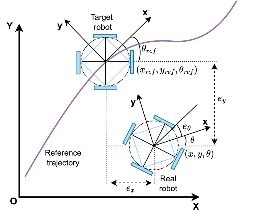
Figure 3: Trajectory tracking error for Omni-drive robot

Similarly, we use $[v_{ref}(nt_{s}),\omega_{ref}(nt_{s})]$ to represent reference linear and angular velocity at each sampling time which is given as,

$$\begin{cases}v_{ref}(nt_{s})=\frac{\sqrt{(\Delta x_{ref}(nt_{s}))^{2}+(\Delta y_{ref}(nt_{s}))^{2}}}{t_{s}}\\ \omega_{ref}(nt_{s})=\frac{\theta_{ref}(nt_{s})-\theta_{ref}((n-1)t_{s})}{t_{s}}\end{cases}$$ (8)

such that,

$$\begin{cases}\Delta y_{ref}(nt_{s})=y_{ref}(nt_{s})-y_{ref}((n-1)t_{s})\\ \Delta x_{ref}(nt_{s})=x_{ref}(nt_{s})-x_{ref}((n-1)t_{s})\end{cases}$$ (9)

In order to track the generated waypoints, the robot position state must also be known in global coordinate system. It is denoted as $\mathbf{X}(T)$ which compose of sequence of pose coordinates of real robot calculated at each sampling interval given by $[x(nt_{s}),y(nt_{s}),\theta(nt_{s})]$. The whole process can be seen in Fig. 3.

4.1 FuzzyPID controller

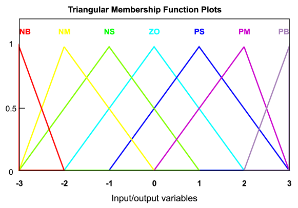
Figure 4: The range of triangular membership function are adjusted based on input and output variables. Both input variables $e$ and $de$ are in the range between -3 to 3. For output variables ($kp,ki,kd$), range is adjusted in between -0.3 to 0.3 keeping the structure of membership function similar.

The design of the fuzzy Controller begins with defining input variables $e(k)$ and the change in error $de(k)$. Initially, these are considered as crisp inputs and need to be converted into 7 overlapping fuzzy sets through the process of fuzzification. The universe of discourse for the variables is defined based on the ranges of the input variables. Triangular membership functions are employed for the fuzzification step, where the membership values (degree of truth) are obtained in the range of 0 to 1 on the universe of discourse for the given input values. This process is illustrated in Fig. 4. Fuzzy sets are represented in linguistic form using the set of variables NB, NM, NS, ZO, PS, PM, and PB, where N, Z, H represent Negative, Zero, and Positive respectively, and B, M, S, O represent Big, Medium, Small, and Zero respectively. The next step involves designing the Mamdani-based fuzzy inference system, where a set of fuzzy rules is defined based on the relationship between fuzzy input sets ($e(k)$ and $de(k)$) and output parameters ($kp,ki,kd$). These rules are formulated by control engineers based on their experience with various system responses. In this context, we establish 49 rules for each fuzzyPID output parameter, drawing reference from the work in [28]. A fuzzy rule takes the form of an IF(antecedent)-THEN(consequent) statement, such as ”if $e(k)$ is PB and $de(k)$ is PB, then apply a large negative $kp$ (i.e., NB)”. The process is executed by fuzzy inference engine that employ the max-min composition.

The final step in the design of the fuzzyPID controller is defuzzification process, which involves the conversion of linguistic variables into crisp output values using membership functions. This step is the reverse process of fuzzification, where values between 0 and 1 are converted using the Center of Gravity (COG) defuzzification technique. Ultimately, we obtain changes in the PID parameters, which are added to the previous PID parameters to continuously track the reference values, expressed as $K_{pid}=K_{pid}^{\prime}+\Delta K_{pid}$. The entire fuzzyPID controller is implemented in Simulink, as illustrated in Fig. 5.

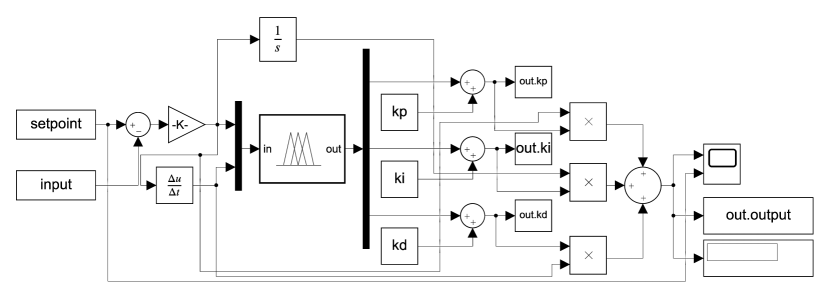
Figure 5: Simulink model of fuzzyPID

Now, tracking the reference trajectory involves calculating the distance and direction errors from robot pose to target reference as,

$$\begin{cases}dr=\sqrt{e_{x}^{2}+e_{y}^{2}},\ dr\geq threshold\\ d\alpha=\tan^{-1}\left(\frac{y_{ref}-y}{x_{ref}-x}\right)-\theta,\ -\pi\leq d\alpha\leq\pi\end{cases}$$ (10)

such that $e_{x}=x_{ref}-x$ and $e_{y}=y_{ref}-y$. The direction error $d\alpha$ forces the robot to follow the target robot with linear velocity $v$ as fuzzyPID($dr$). But, this leads to problem of drifting heading angle which in our case is designed to follow the reference heading angle defined in Equation (7). So, we need addition angular velocity($\omega$) to do the following task which is calculated as fuzzyPID($e_{\theta}$) such that $e_{\theta}=\theta_{ref}-\theta$. Thus, the global velocity of robot is formulated as $[v\cos(d\alpha),v\sin(d\alpha),\omega]$ which is finally passed through the inverse kinematics model to compute individual wheel velocity.

4.2 Non-linear MPC

The Non-linear Model Predictive Controller (NMPC) is an optimization technique that employs the non-linear classical kinematics model to predict the future behavior of a mobile robot within bounded physical constraints on both state variables and control inputs. The cost function is formulated by integrating the tracking error between the predicted states and the true output states within a finite prediction horizon $N_{p}$ in a sliding mode fashion. Additionally, it includes a term for minimizing the control input error for the target robot velocity. Subsequently, the cost function is processed through a non-linear solver [29], thereby achieving optimal robot states and control sequences for the next $N_{p}$ prediction horizon. These optimal robot states are closer to the desired path based on the corresponding applied control sequences. Next, we advance one sample time ahead to compute the target direction angle from the first state. Similarly, we consider the first control input velocity, and these steps are repeated for each sampling period with the shifted horizon.

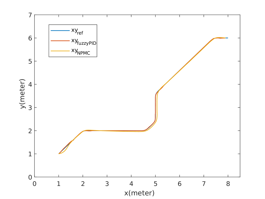
Figure 6: Comparison of tracking performance of pose(XY) for both fuzzyPID and NMPC with prediction horizon of 15 with a total tracking time of 30 seconds

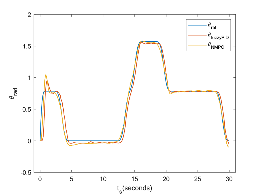
Figure 7: Comparison of tracking performance of pose($\theta$) for both fuzzyPID and NMPC with prediction horizon of 15 with a total tracking time of 30 seconds

Here, discrete time non-linear model is used to predict the evolution of future states for the mobile robot. Given $N_{p}$ prediction horizon, following mathematical equation is used to compute state at each sample period $k=nt_{s}$.

$${\mathbf{x}}(k+1\mid k)={\mathbf{x}}(k\mid k)+t_{s}\dot{{\mathbf{x}}}(k\mid k)$$ (11)

Given that,

$$\dot{{\mathbf{x}}}(k) =f({\mathbf{x}}(k),{u}(k))\ s.t.\ {\mathbf{x}}(k)\in X,{u}(k)\in U,\forall{k}\geq 0$$

$$=[v(k)cos(\theta(k)),v(k)sin(\theta(k)),\dot{\theta}(k)]^{T}$$ (12)

where, $\mathbf{x}(k)\in\mathbb{R}^{n}$ and $u(k)\in\mathbb{R}^{m}$ are the state and control vector respectively. Subsequently, we calculate the error between the robot predicted states and reference trajectory as,

$$\left\{\begin{array}[]{c}\mathbf{e}(k\mid k)=\mathbf{\bar{x}}(k\mid k)-\mathbf{x}_{ref}(k\mid k)\\ \vdots\\ \mathbf{e}\left(k+N_{p}\mid k\right)=\mathbf{\bar{x}}\left(k+N_{p}\mid t\right)-\mathbf{x}_{ref}\left(k+N_{p}\mid k\right)\end{array}\right.$$ (13)

$$\mathbf{x}_{ref}(k\mid k)=\left[\begin{array}[]{lll}x_{ref}(k\mid k)&y_{ref}(k\mid k)&\theta_{ref}(k\mid k)\end{array}\right]^{\mathrm{T}}$$ (14)

where, $\mathbf{\bar{x}}(k\mid k)=\mathbf{x}(k)$ which is robot initial position state. Given target velocity, we also define our objective to minimize the control input error over the finite control horizon of length $N_{p}-1$ as defined by equation,

$$\left\{\begin{aligned} \Delta\mathbf{u}(k\mid k)&=\mathbf{\bar{u}}(k\mid k)-\mathbf{u_{ref}}(k\mid k)\\ &\vdots\\ \Delta\mathbf{u}(k+i+1\mid k)&=\mathbf{\bar{u}}(k+i+1\mid k)-\mathbf{u_{ref}}(k+i+1\mid k)\\ &\vdots\\ \Delta\mathbf{u}\left(k+N_{p}-1\mid k\right)&=\mathbf{\bar{u}}\left(k+N_{p}-1\mid k\right)-\mathbf{u_{ref}}\left(k+N_{p}-1\mid k\right)\end{aligned}\right.$$ (15)

$$\mathbf{u}_{ref}(k\mid k)=\left[\begin{array}[]{lll}v_{ref}(k\mid k)&\omega_{ref}(k\mid k)\end{array}\right]^{\mathrm{T}}$$ (16)

Our objective cost function to be optimized is given as,

$$w^{*}=\min J_{w}(\mathbf{e}(k\mid k),\Delta\mathbf{u}(k\mid k)=\sum_{k=0}^{N_{p}}\|\mathbf{e}(k+i\mid k)\|_{\mathbf{Q}}^{2}+\sum_{k=0}^{N_{p}-1}\|\Delta\mathbf{u}(k+i\mid k)\|_{\mathbf{R}}^{2}$$ (17)

subject to equality constraints:

$$\mathbf{g}_{2}(\mathbf{w})=\left[\begin{array}[]{c}\overline{\mathbf{x}}(k)-\mathbf{x}(k)\\ \mathbf{f}\left(\mathbf{x}(k),\mathbf{u}(k)\right)-\mathbf{x}(k+1)\\ \vdots\\ \mathbf{f}\left(\mathbf{x}(k+N_{p}-1),\mathbf{u}(k+N_{p}-1)\right)-\mathbf{x}(k+N_{p})\end{array}\right]=0$$ (18)

where, $w=\left[\begin{array}[]{lllll}\mathbf{u}_{0}&\cdots&\mathbf{u}_{N_{p}-1},\mathbf{x}_{0}&\cdots&\mathbf{x}_{N_{p}}\end{array}\right]$ are problem decision variables which need to be solved. Also the weight matrix $\mathbf{Q}\in\mathbb{R}^{n*n}$ and $\mathbf{R}\in\mathbb{R}^{m*m}$ are tuned for the better accuracy and smooth control inputs. Now, we calculate next output state $\mathbf{x_{1}}$ based on optimal control input $\mathbf{u_{0}}$. We extract third element from evolved state which acts as the target direction angle for the Omni-drive robot. Similarly, linear and angular velocity corresponding to first input vector $\mathbf{u_{0}}$ acts as control inputs which drives the robot to reference pose coordinates.

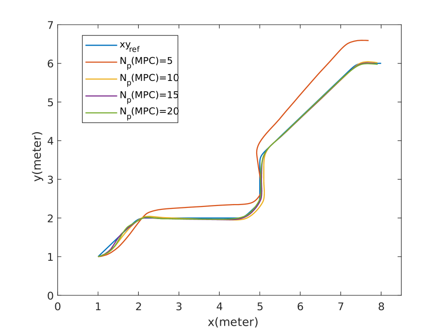
Figure 8: Comparison of tracking performance of pose(XY) for NMPC with different prediction horizon values with total tracking time of 20 seconds

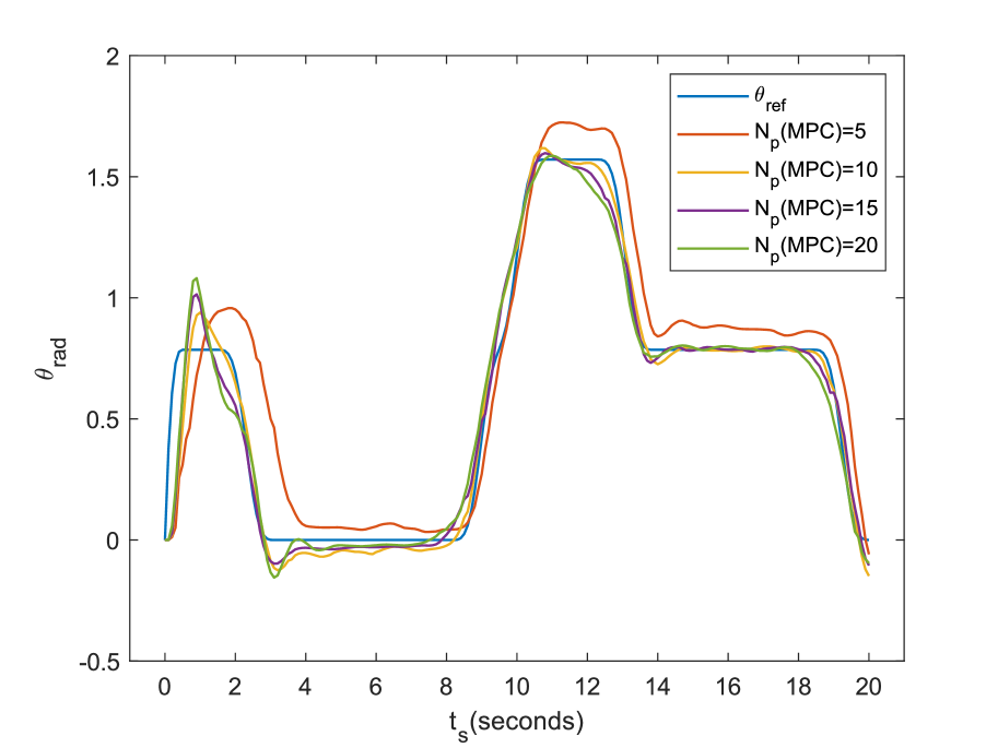
Figure 9: Comparison of tracking performance of pose($\theta$) for NMPC with different prediction horizon values with total tracking time of 20 seconds

5 Simulation setup

We conduct trajectory tracking experiments using CoppeliaSim, with our primary objective being the comparison of tracking accuracy between both controllers while keeping the sampling time constant. The tracking performance is simulated over a fixed time intervals of 20 and 30 seconds for the generated trajectory, and the results obtained are plotted for a fair comparison. The reference and actual 2D-pose values for both the controllers are shown in Fig. 7 and 7. For NMPC, we use a prediction horizon value of 15. It is crucial to note that altering the prediction horizon value has adverse effects on the controller’s efficiency, as illustrated in Fig. 9 and 9. The accuracy of the controller is also dependent on the number of intermediate poses sampled within the given tracking time. In this trajectory experiment, we choose the parameters as, $\mathbf{Q}=15\mathbb{I}_{3}$, $\mathbf{R}=\mathbb{I}_{2}$, $t_{s}=0.1s$, $v_{max}=1.5m/s$, $\omega_{max}=3.14rad/s$.

We do not take hardware constraints into account as limitations for our simulation platforms. Mean Cross-track Error (ME) and Mean Absolute Error (MAE) metrics serve as the evaluation criteria for judging our results. ME is calculated by averaging the Euclidean distance between the target pose and the real pose at each sampling period. Similarly, we calculate the average value of all absolute deviations between the reference heading angle and the robot heading angle for MAE. Lower error values correspond to better tracking accuracy. Furthermore, we compare the tracking results for different prediction horizon values ($N_{p}$) in the case of Non-linear Model Predictive Control.

Table 1: Comparison of tracking error of omni drive robot for both fuzzyPID and NMPC

	fuzzyPID			NPMC($N_{p}=15$)
Tracking time		ME($XY$)	MAE($\theta$)		ME($XY$)	MAE($\theta$)
20 seconds		0.0712 m	0.0793 rad		0.0529 m	0.0564 rad
30 seconds		0.0499 m	0.0613 rad		0.0439 m	0.0391 rad

6 Comparison of fuzzyPID and NMPC

Table 1 presents the tracking error for both fuzzyPID and NMPC with a prediction horizon value of 15. The NMPC controller achieves a lower error compared to fuzzyPID in both metrics. As the tracking time increases, a corresponding improvement in tracking accuracy is observed for both controllers. FuzzyPID is identified as more computationally efficient than NMPC, albeit at the expense of tracking accuracy.

Conversely, the performance of NMPC is contingent upon selecting a suitable value for the prediction horizon, resulting in a significant impact on the designed controller’s performance. Opting for a lower prediction horizon value leads to suboptimal control actions, rendering the controller less adept at handling the complex dynamics of the system and resulting in lower accuracy. Conversely, a larger prediction horizon increases system complexity and results in a slower response. Furthermore, it introduces a higher risk of overfitting to the prediction model, subsequently yielding sub-optimal results. The error for different values of the prediction horizon is illustrated in Fig. 10.

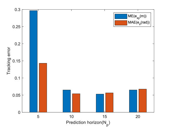
Figure 10: Comparison of tracking error of robot pose for NMPC with different prediction horizon values with total tracking time of 20 seconds

7 Conclusions

In this study, we propose a comprehensive framework for developing a trajectory tracking methodology in a 4-wheel Omni-drive robot. This scheme involves deriving the kinematic model, creating an obstacle-free path, followed by a path-smoothing algorithm. Subsequently, we design two popular control methods, namely fuzzyPID and NPMC, for achieving robust path tracking. The entire setup is simulated, and we compare tracking performance by calculating the cross-track error for both controllers.

The results indicate that NPMC outperforms fuzzyPID, albeit with a trade-off in computational complexity. Conversely, the simplicity of fuzzyPID makes it applicable in a wide variety of controller applications. We also assess the effectiveness of NMPC for different values of the prediction horizon in the stability control of our robot.

In a nutshell, the proposed approaches can be useful for a variety of control and robotics tasks, aiming to improve the accuracy and throughput of the system.

References

- \bibcommenthead
- Shabalina et al. [2018] Shabalina, K., Sagitov, A., Magid, E.: Comparative analysis of mobile robot wheels design. In: 2018 11th International Conference on Developments in eSystems Engineering (DeSE), pp. 175–179 (2018). IEEE
- Taheri and Zhao [2020] Taheri, H., Zhao, C.X.: Omnidirectional mobile robots, mechanisms and navigation approaches. Mechanism and Machine Theory 153, 103958 (2020)
- Karur et al. [2021] Karur, K., Sharma, N., Dharmatti, C., Siegel, J.E.: A survey of path planning algorithms for mobile robots. Vehicles 3(3), 448–468 (2021)
- Ravankar et al. [2018] Ravankar, A., Ravankar, A.A., Kobayashi, Y., Hoshino, Y., Peng, C.-C.: Path smoothing techniques in robot navigation: State-of-the-art, current and future challenges. Sensors 18(9), 3170 (2018)
- Somwanshi et al. [2019] Somwanshi, D., Bundele, M., Kumar, G., Parashar, G.: Comparison of fuzzy-pid and pid controller for speed control of dc motor using labview. Procedia Computer Science 152, 252–260 (2019)
- Lee et al. [2018] Lee, K., Im, D.-Y., Kwak, B., Ryoo, Y.-J., et al.: Design of fuzzy-pid controller for path tracking of mobile robot with differential drive. International Journal of Fuzzy Logic and Intelligent Systems 18(3), 220–228 (2018)
- Jiang and Jiang [2012] Jiang, W., Jiang, X.: Design of an intelligent temperature control system based on the fuzzy self-tuning pid. Procedia Engineering 43, 307–311 (2012)
- Bansal and Narvey [2013] Bansal, U.K., Narvey, R.: Speed control of dc motor using fuzzy pid controller. Advance in Electronic and Electric Engineering 3(9), 1209–1220 (2013)
- Chao et al. [2019] Chao, C.-T., Sutarna, N., Chiou, J.-S., Wang, C.-J.: An optimal fuzzy pid controller design based on conventional pid control and nonlinear factors. Applied Sciences 9(6), 1224 (2019)
- Nour et al. [2007] Nour, M., Ooi, J., Chan, K.: Fuzzy logic control vs. conventional pid control of an inverted pendulum robot. In: 2007 International Conference on Intelligent and Advanced Systems, pp. 209–214 (2007). IEEE
- Alouache and Wu [2018] Alouache, A., Wu, Q.: Fuzzy logic pd controller for trajectory tracking of an autonomous differential drive mobile robot (ie quanser qbot). Industrial Robot: An International Journal 45(1), 23–33 (2018)
- Hashemi et al. [2011] Hashemi, E., Jadidi, M.G., Jadidi, N.G.: Model-based pi–fuzzy control of four-wheeled omni-directional mobile robots. Robotics and Autonomous Systems 59(11), 930–942 (2011)
- Abiyev et al. [2017] Abiyev, R.H., Günsel, I.S., Akkaya, N., Aytac, E., Çağman, A., Abizada, S.: Fuzzy control of omnidirectional robot. Procedia Computer Science 120, 608–616 (2017)
- Vu et al. [2021] Vu, T.M., Moezzi, R., Cyrus, J., Hlava, J.: Model predictive control for autonomous driving vehicles. Electronics 10(21), 2593 (2021)
- Maurović et al. [2011] Maurović, I., Baotić, M., Petrović, I.: Explicit model predictive control for trajectory tracking with mobile robots. In: 2011 IEEE/ASME International Conference on Advanced Intelligent Mechatronics (AIM), pp. 712–717 (2011). IEEE
- Liu et al. [2022] Liu, X., Wang, W., Li, X., Liu, F., He, Z., Yao, Y., Ruan, H., Zhang, T.: Mpc-based high-speed trajectory tracking for 4wis robot. ISA transactions 123, 413–424 (2022)
- Kanjanawanishkul and Zell [2009] Kanjanawanishkul, K., Zell, A.: Path following for an omnidirectional mobile robot based on model predictive control. In: 2009 IEEE International Conference on Robotics and Automation, pp. 3341–3346 (2009). IEEE
- Yang et al. [2018] Yang, H., Guo, M., Xia, Y., Cheng, L.: Trajectory tracking for wheeled mobile robots via model predictive control with softening constraints. IET Control Theory & Applications 12(2), 206–214 (2018)
- Nascimento et al. [2018] Nascimento, T.P., Dórea, C.E.T., Gonçalves, L.M.G.: Nonlinear model predictive control for trajectory tracking of nonholonomic mobile robots: A modified approach. International Journal of Advanced Robotic Systems 15(1), 1729881418760461 (2018)
- Pacheco and Luo [2015] Pacheco, L., Luo, N.: Testing pid and mpc performance for mobile robot local path-following. International Journal of Advanced Robotic Systems 12(11), 155 (2015)
- Mayne [2014] Mayne, D.Q.: Model predictive control: Recent developments and future promise. Automatica 50(12), 2967–2986 (2014)
- Bai et al. [2019] Bai, G., Meng, Y., Liu, L., Luo, W., Gu, Q., Liu, L.: Review and comparison of path tracking based on model predictive control. Electronics 8(10), 1077 (2019)
- Conceição et al. [2007] Conceição, A.S., Oliveira, H.P., Silva, A.S., Oliveira, D., Moreira, A.P.: A nonlinear model predictive control of an omni-directional mobile robot. In: 2007 IEEE International Symposium on Industrial Electronics, pp. 2161–2166 (2007). IEEE
- Wang et al. [2018] Wang, C., Liu, X., Yang, X., Hu, F., Jiang, A., Yang, C.: Trajectory tracking of an omni-directional wheeled mobile robot using a model predictive control strategy. Applied Sciences 8(2), 231 (2018)
- Grüne et al. [2017] Grüne, L., Pannek, J., Grüne, L., Pannek, J.: Nonlinear Model Predictive Control. Springer, ??? (2017)
- Baede [2006] Baede, T.: Motion control of an omnidirectional mobile robot. Traineeship report DCT 2006 (2006)
- Jing and Yang [2018] Jing, X., Yang, X.: Application and improvement of heuristic function in a* algorithm. In: 2018 37th Chinese Control Conference (CCC), pp. 2191–2194 (2018). IEEE
- Xu and Wang [2017] Xu, X., Wang, Q.: Speed control of hydraulic elevator by using pid controller and self-tuning fuzzy pid controller. In: 2017 32nd Youth Academic Annual Conference of Chinese Association of Automation (YAC), pp. 812–817 (2017). IEEE
- Andersson et al. [2019] Andersson, J.A., Gillis, J., Horn, G., Rawlings, J.B., Diehl, M.: Casadi: a software framework for nonlinear optimization and optimal control. Mathematical Programming Computation 11, 1–36 (2019)