PolyominoIdeals: a package for Macaulay2 to work with the inner $2$-minor ideals of collections of cells

Abstract.

Let $\mathcal{P}$ be a collection of cells and $I_{\mathcal{P}}$ be the associated ideal of inner $2$-minors as defined by A. A. Qureshi in 2012. In this paper, we provide a description of the package PolyominoIdeals for the computer algebra software Macaulay2. More precisely, this package provides some functions that allow to define the ideal $I_{\mathcal{P}}$ in Macaulay2 and to compute its algebraic invariants or verifying its algebraic properties. We explain the usage of these functions and also give some examples.

1. Introduction

An unitary square in $\mathbb{Z}^{2}$, whose vertices have integer coordinates, is said to be a cell. Considering collections of cells in the plane, it is possible to create many geometric objects having a different shapes. A particular class of collections of cells consists of polyominoes. A polyomino is a finite collection of unitary squares joined edge by edge. This term was coined by S. W. Golomb in 1953 and such configurations have been studied mainly in Combinatorial Mathematics, for instance in some tiling problems of the plane. In 2012 A.A. Qureshi (see [28]) defined a polyomino ideal attached to a polyomino $\mathcal{P}$, as the ideal generated by all inner 2-minors of $\mathcal{P}$ in the polynomial ring $S_{\mathcal{P}}$, that is the polynomial ring over a field $K$ in the variables $x_{v}$, for all $v$ vertices of cells in $\mathcal{P}$. Such an ideal is called the polyomino ideal of $\mathcal{P}$ and it is denoted by $I_{\mathcal{P}}$. For more details see [28]. The study of the main algebraic properties of the quotient ring $K[\mathcal{P}]=S_{\mathcal{P}}/I_{\mathcal{P}}$, depending on the shape of $\mathcal{P}$, has become an exciting line of research. Many authors have focused their attention about that, see [2], [3], [4], [5], [6], [7], [8], [9], [10], [14], [16], [17], [18], [21], [22], [24], [25], [26], [29], [30], [31], [32].
In this paper, we provide a description of the package PolyominoIdeals for the computer algebra software Macaulay2. The purpose of this package is to allow the definition and manipulation of the binomial ideals attached to collections of cells, inside the computer algebra software. More precisely, encoding a fixed collection of cells by a list of lists containing the diagonal corners of each cell, the package provides three functions. The function polyoIdeal allows to define the inner $2$-minor ideal of $\mathcal{P}$. For this function, we also give three options. The option RingChoice allows one to choose between two rings having two different monomial orders: one is the lexicographic order induced by the natural partial order on $V(\mathcal{P})$; the other one is the monomial order $<$ given in [19] for bipartite graphs, that can be induced in a polyomino as shown in [28], where one also can deduce that, for a convex polyomino $\mathcal{P}$, the generators of the ideal $I_{\mathcal{P}}$ form the reduced Gröbner basis with respect to $<$. For the other two options, the first one is Field which allows changing the base field $K$ in the base polynomial ring of $I_{\mathcal{P}}$, and the second is TermOder, which allows replacing the lexicographic order by other term orders when RingChoice is defined in the first way as described above. For the other functions, we have polyoToric, which allows generating the toric ideal defined in [25]. The third function polyoMatrix gives the matrix attached to $\mathcal{P}$, that is the matrix whose set of all $2$-minors consists of the set of generators of the ideal $I_{\mathcal{P}}$. The paper is arranged as follows. In Section 2 we introduce and explain in detail the main mathematical definitions for collections of cells and the associated ideals, needed for what we describe in this work. In Section 3 we describe the functions and the related options and we show several examples of them. In Section 4 we explain a useful trick that allows getting the list encoding the collection of cells using GeoGebra.

2. Mathematical background on polyominoes and polyomino ideals

Let $(i,j),(k,l)\in\mathbb{Z}^{2}$. We say that $(i,j)\leq(k,l)$ if $i\leq k$ and $j\leq l$. Consider $a=(i,j)$ and $b=(k,l)$ in $\mathbb{Z}^{2}$ with $a\leq b$, the set $[a,b]=\{(m,n)\in\mathbb{Z}^{2}:i\leq m\leq k,\ j\leq n\leq l\}$ is called an interval of $\mathbb{Z}^{2}$. In addition, if $i<k$ and $j<l$ then $[a,b]$ is a proper interval. In such a case we say $a,b$ the diagonal corners of $[a,b]$ and $c=(i,l)$, $d=(k,j)$ the anti-diagonal corners of $[a,b]$. If $j=l$ (or $i=k$) then $a$ and $b$ are in horizontal (or vertical) position. We denote by $]a,b[$ the set $\{(m,n)\in\mathbb{Z}^{2}:i<m<k,\ j<n<l\}$. A proper interval $C=[a,b]$ with $b=a+(1,1)$ is called a cell of ${\mathbb{Z}}^{2}$; moreover, the elements $a$, $b$, $c$ and $d$ are called respectively the lower left, upper right, upper left and lower right corners of $C$. The sets $\{a,c\}$, $\{c,b\}$, $\{b,d\}$ and $\{a,d\}$ are the edges of $C$. We put $V(C)=\{a,b,c,d\}$ and $E(C)=\{\{a,c\},\{c,b\},\{b,d\},\{a,d\}\}$. Let $\mathcal{S}$ be a non-empty collection of cells in $\mathbb{Z}^{2}$. The set of the vertices and of the edges of $\mathcal{S}$ are respectively $V(\mathcal{S})=\bigcup_{C\in\mathcal{S}}V(C)$ and $E(\mathcal{S})=\bigcup_{C\in\mathcal{S}}E(C)$, while $\mathop{\rm rank}\nolimits\mathcal{S}$ is the number of cells belonging to $\mathcal{S}$. If $C$ and $D$ are two distinct cells of $\mathcal{S}$, then a walk from $C$ to $D$ in $\mathcal{S}$ is a sequence $\mathcal{C}:C=C_{1},\dots,C_{m}=D$ of cells of ${\mathbb{Z}}^{2}$ such that $C_{i}\cap C_{i+1}$ is an edge of $C_{i}$ and $C_{i+1}$ for $i=1,\dots,m-1$. In addition, if $C_{i}\neq C_{j}$ for all $i\neq j$, then $\mathcal{C}$ is called a path from $C$ to $D$. Two cells $C$ and $D$ are called connected in $\mathcal{S}$ if there exists a path of cells in $\mathcal{S}$ from $C$ to $D$. A connected collection of cells $\mathcal{P}$ is called polyomino.
Let $\mathcal{P}$ be a non-empty, finite collection of cells in $\mathbb{Z}^{2}$, $\mathcal{P}$ is called weakly connected if for any two cells $C$ and $D$ in $\mathcal{P}$ there exists a sequence of cells $\mathcal{C}:C=C_{1},\dots,C_{m}=D$ of $\mathcal{P}$ such that $V(C_{i})\cap V(C_{i+1})\neq\emptyset$ for all $i=1,\dots,m-1$. A subset of cells $\mathcal{P}^{\prime}$ of $\mathcal{P}$ is called a connected component of $\mathcal{P}$ if $\mathcal{P}^{\prime}$ is a polyomino and it is maximal with respect to the set inclusion, that is if $A\in\mathcal{P}\setminus\mathcal{P}^{\prime}$ then $\mathcal{P}^{\prime}\cup\{A\}$ is not a polyomino. For instance, see Figure 1 (A). Observe trivially that every polyomino is a weakly connected collection of cells. For instance, see Figure 1 (B).

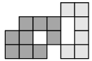
(a)

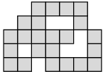
(b)

Figure 1.

A weakly connected collection $\mathcal{P}$ of cells is row convex, if the horizontal cell interval $[A,B]$ is contained in $\mathcal{P}$ for any two cells $A$ and $B$ of $\mathcal{P}$ whose lower left corners are in a horizontal position. Similarly one defines column convex. $\mathcal{P}$ is called convex if it is row and column convex. A polyomino $\mathcal{P}$ is simple if for any two cells $C$ and $D$ not in $\mathcal{P}$ there exists a path of cells not in $\mathcal{P}$ from $C$ to $D$. A finite collection of cells $\mathcal{H}$ not in $\mathcal{P}$ is a hole of $\mathcal{P}$ if any two cells of $\mathcal{H}$ are connected in $\mathcal{H}$ and $\mathcal{H}$ is maximal with respect to set inclusion. For example, the polyomino in Figure 1 (A) is not simple with three holes. Obviously, each hole of $\mathcal{P}$ is a simple polyomino and $\mathcal{P}$ is simple if and only if it has not any hole.
Let $A$ and $B$ be two cells of $\mathbb{Z}^{2}$ with $a=(i,j)$ and $b=(k,l)$ as the lower left corners of $A$ and $B$ and $a\leq b$. A cell interval $[A,B]$ is the set of the cells of $\mathbb{Z}^{2}$ with lower left corner $(r,s)$ such that $i\leqslant r\leqslant k$ and $j\leqslant s\leqslant l$. If $(i,j)$ and $(k,l)$ are in horizontal (or vertical) position, we say that the cells $A$ and $B$ are in horizontal (or vertical) position.
Let $A$ and $B$ be two cells of a polyomino $\mathcal{P}$ in a vertical or horizontal position. The cell interval $[A,B]$, containing $n>1$ cells, is called a block of $\mathcal{P}$ of rank n if all cells of $[A,B]$ belong to $\mathcal{P}$. The cells $A$ and $B$ are called extremal cells of $[A,B]$. Moreover, a block $\mathcal{B}$ of $\mathcal{P}$ is maximal if there does not exist any block of $\mathcal{P}$ which contains properly $\mathcal{B}$. It is clear that an interval of ${\mathbb{Z}}^{2}$ identifies a cell interval of ${\mathbb{Z}}^{2}$ and vice versa, hence we associate to an interval $I$ of ${\mathbb{Z}}^{2}$ the corresponding cell interval denoted by $\mathcal{P}_{I}$. A proper interval $[a,b]$ is called an inner interval of $\mathcal{P}$ if all cells of $\mathcal{P}_{[a,b]}$ belong to $\mathcal{P}$. We denote by $\mathcal{I}(\mathcal{P})$ the set of all inner intervals of $\mathcal{P}$. An interval $[a,b]$ with $a=(i,j)$, $b=(k,j)$ and $i<k$, is called a horizontal edge interval of $\mathcal{P}$ if the sets $\{(\ell,j),(\ell+1,j)\}$ are edges of cells of $\mathcal{P}$ for all $\ell=i,\dots,k-1$. In addition, if $\{(i-1,j),(i,j)\}$ and $\{(k,j),(k+1,j)\}$ do not belong to $E(\mathcal{P})$, then $[a,b]$ is called a maximal horizontal edge interval of $\mathcal{P}$. We define similarly a vertical edge interval and a maximal vertical edge interval.
Let $\mathcal{P}$ be a collection of cells, we set $S_{\mathcal{P}}=K[x_{v}|v\in V(\mathcal{P})]$, where $K$ is a field. If $[a,b]$ is an inner interval of $\mathcal{P}$, with $a$,$b$ and $c$,$d$ respectively diagonal and anti-diagonal corners, then the binomial $x_{a}x_{b}-x_{c}x_{d}$ is called an inner 2-minor of $\mathcal{P}$. $I_{\mathcal{P}}$ denotes the ideal in $S_{\mathcal{P}}$ generated by all the inner 2-minors of $\mathcal{P}$ and is called the polyomino ideal of $\mathcal{P}$, if $\mathcal{P}$ is a polyomino. The quotient ring $K[\mathcal{P}]=S_{\mathcal{P}}/I_{\mathcal{P}}$ is called the coordinate ring of $\mathcal{P}$.

3. Functions in the package PolyoIdeals

In this section we describe the functions included in the package PolyominoIdeals.m2 developed for Macaulay2 ([13]). First of all, consider that a collection of cells $\mathcal{P}$ is encoded, for the package, with a list of lists, where each list represents a cell of the collection and contains two lists representing the diagonal corners of the cell, the first for the lower left corner, the second for the upper right corner. For instance, the collection of cells in Figure 2 is encoded with the list Q = {{{1, 1}, {2, 2}}, {{2, 1}, {3, 2}}, {{3, 1}, {4, 2}}, {{2, 2}, {3, 3}}, {{3, 2}, {4, 3}}, {{2, 3}, {3, 4}}}.

3.1. polyoIdeal function

Let $\mathcal{P}$ be a polyomino and $I_{\mathcal{P}}$ be the polyomino ideal associated to $\mathcal{P}$. The polyoIdeal function available in the PolyominoIdeals package gives the output as the generators of polyomino ideal $I_{\mathcal{P}}$. The polynomial ring defined as $S_{\mathcal{P}}=K[x_{v}:v\in V(\mathcal{P})]$ is auto-declared in the polyoIdeal function and can be accessed with the command ring(polyoIdeal(Q)), where Q is the input list which comprises of the diagonal corners of each cell in $\mathcal{P}$.

Example 3.1.

Consider the polyomino on $6$ cells shown in Figure 2. Observe that the inner intervals are $[A,F],[A,G],[A,H],[B,G],[B,H],[B,J],[B,K],[B,M],[C,H],[C,K].[F,J],$ $[F,K],[F,M],[G,K],[I,M]$ and, by definition of the polyomino ideal, the generators correspond to the binomials associated with the 14 inner intervals listed above.

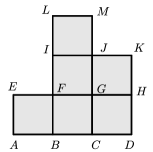
Figure 2. A polyomino.

Fixing the lower left corner $A$ as $(1,1)$ we embed the polyomino with the list $Q=\{\{\{1,1\},\{2,2\}\},\{\{2,1\},\{3,2\}\},\{\{3,1\},\{4,2\}\},\{\{2,2\},\{3,3\}\},\{\{3,2\},\{4,3\}\},\{\{2,3\},\{3,4\}\}\}$. Using the polyoIdeal(Q) function we obtain the binomials that generate the polyomino ideal.

⬇

Macaulay2, version 1.20

with packages: ConwayPolynomials, Elimination, IntegralClosure,

InverseSystems, Isomorphism, LLLBases, MinimalPrimes, OnlineLookup,

PrimaryDecomposition, ReesAlgebra, Saturation, TangentCone

i1 : loadPackage ”PolyominoIdeals”;

i2 : Q={{{1, 1}, {2, 2}}, {{2, 1}, {3, 2}}, {{3, 1}, {4, 2}}, {{2, 2}, {3, 3}},

{{3, 2}, {4, 3}}, {{2, 3}, {3, 4}}};

i3 : I=polyoIdeal(Q);

i4 : g = gens I

o4 : | x_(4,3)x_(3,2)-x_(4,2)x_(3,3) x_(2,2)x_(1,1)-x_(2,1)x_(1,2)

—————————————————————————

x_(4,3)x_(2,1)-x_(4,1)x_(2,3) x_(3,2)x_(2,1)-x_(3,1)x_(2,2)

—————————————————————————

x_(4,3)x_(2,2)-x_(4,2)x_(2,3) x_(3,3)x_(2,1)-x_(3,1)x_(2,3)

—————————————————————————

x_(4,2)x_(1,1)-x_(4,1)x_(1,2) x_(3,4)x_(2,1)-x_(3,1)x_(2,4)

—————————————————————————

x_(3,3)x_(2,2)-x_(3,2)x_(2,3) x_(4,2)x_(3,1)-x_(4,1)x_(3,2)

—————————————————————————

x_(3,4)x_(2,2)-x_(3,2)x_(2,4) x_(3,2)x_(1,1)-x_(3,1)x_(1,2)

—————————————————————————

x_(4,3)x_(3,1)-x_(4,1)x_(3,3) x_(3,4)x_(2,3)-x_(3,3)x_(2,4)

—————————————————————————

x_(4,2)x_(2,1)-x_(4,1)x_(2,2) |

3.2. polyoMatrix function

Let $\mathcal{P}$ be a collection of cells and $[(p,q),(r,s)]$ be the smallest interval of ${\mathbb{N}}^{2}$ containing $\mathcal{P}$. The matrix $M(\mathcal{P})$ has $s-q+1$ rows and $r-p+1$ columns with $M(\mathcal{P})_{i,j}=x_{(i,j)}$ if $(i,j)$ is a vertex of $\mathcal{P}$, otherwise it is zero.

Example 3.2.

Consider the same polyomino given in Figure 2 encoded by $Q=\{\{\{1,1\},\{2,2\}\},\{\{2,1\},\{3,2\}\},\{\{3,1\},\{4,2\}\},\{\{2,2\},\{3,3\}\},\{\{3,2\},\{4,3\}\},\{\{2,3\},\{3,4\}\}\}$. The associated matrix is obtained using polyoMatrix function.

⬇

Macaulay2, version 1.20

with packages: ConwayPolynomials, Elimination, IntegralClosure,

InverseSystems, Isomorphism, LLLBases, MinimalPrimes, OnlineLookup,

PrimaryDecomposition, ReesAlgebra, Saturation, TangentCone

i1 : loadPackage ”PolyominoIdeals”;

i2 : Q={{{1, 1}, {2, 2}}, {{2, 1}, {3, 2}}, {{3, 1}, {4, 2}}, {{2, 2}, {3, 3}},

{{3, 2}, {4, 3}}, {{2, 3}, {3, 4}}};

i3 : M=polyoMatrix(Q);

o3 : | 0 x_(2,4) x_(3,4) 0 |

| 0 x_(2,3) x_(3,3) x_(4,3) |

| x_(1,2) x_(2,2) x_(3,2) x_(4,2) |

| x_(1,1) x_(2,1) x_(3,1) x_(4,1) |

The associated matrix for a collection of cells can help to order the variables to define a polynomial ring with another monomial order. In particular, this function is fundamental for coding the option when RingChoice has a different value by $1$ (see Subsection 3.5). Also, the ideal generated by all the inner $2$-minors of this matrix is the same polyomino ideal defined earlier.

3.3. polyoToric function

Let $\mathcal{P}$ be a weakly connected collection of cells. We introduce a suitable toric ideal attached to $\mathcal{P}$ based on that one given in [25] for polyominoes. Consider the following total order on $V(\mathcal{P})$: $a=(i,j)>b=(k,l)$, if $i>k$, or $i=k$ and $j>l$. If $\mathcal{H}$ is a hole of $\mathcal{P}$, then we call the lower left corner $e$ of $\mathcal{H}$ the minimum, with respect to $<$, of the vertices of $\mathcal{H}$. Let $\mathcal{H}_{1},\dots,\mathcal{H}_{r}$ be the holes of $\mathcal{P}$ and $e_{k}=(i_{k},j_{k})$ be the lower left corner of $\mathcal{H}_{k}$. For $k\in K=[r]$, we define the following subset $F_{k}=\{(i,j)\in V(\mathcal{P}):i\leq i_{k},j\leq j_{k}\}$. Denote by $\{V_{i}\}_{i\in I}$ the set of all the maximal vertical edge intervals of $\mathcal{P}$, and by $\{H_{j}\}_{j\in J}$ the set of all the maximal horizontal edge intervals of $\mathcal{P}$. Let $\{v_{i}\}_{i\in I}$, $\{h_{j}\}_{j\in J}$ , and $\{w_{k}\}_{k\in K}$ be three sets of variables. We consider the map

$$\alpha:V(\mathcal{P})\rightarrow K[{h_{i},v_{j},w_{k}}:i\in I,j\in J,k\in K]$$

$$a\rightarrow\prod_{a\in H_{i}\cap V_{j}}h_{i}v_{j}\prod_{a\in F_{k}}w_{k}$$

The toric ring $T_{\mathcal{P}}$ associated to $\mathcal{P}$ is defined as $T_{\mathcal{P}}=K[\alpha(a):a\in V(\mathcal{P})]$. The homomorphism $\psi:S\rightarrow T_{\mathcal{P}}$ with $x_{a}\rightarrow\alpha(a)$ is surjective and the toric ideal $J_{\mathcal{P}}$ is the kernel of $\psi$. Observe that the latter generalizes in a natural way that is given in [3] and [30].

Theorem 3.3 (Theorem 3.3, [3]).

Let $\mathcal{P}$ be a simple and weakly-connected collection of cells. Then $I_{\mathcal{P}}=J_{\mathcal{P}}$.

The same holds for the class of grid polyominoes, defined in Section 4 of [25]. Moreover, with some suitable changes in the choice of the vertices of $\mathcal{P}$ to assign the variable $w$, similar statements can be proved for the classes of closed paths and weakly closed paths (see Section 4-5 of [2] and Section 4 of [3]).

The function PolyoToric(Q,H) provides the toric ideal $J_{\mathcal{P}}$ defined before, where Q is the list encoding the collection of cells and H is the list of the lower left corners of the holes. It provides a nice tool to study the primality of the inner $2$-minor ideals of weakly connected collections of cells. Here we illustrate some examples.

Example 3.4.

Consider the simple and weakly-connected collection $\mathcal{P}$ of cells in Figure 3 (A), encoded by the list Q={{{1, 1}, {2, 2}}, {{2, 2}, {3, 3}}, {{2, 1}, {3, 2}},{{3, 2}, {4, 3}},{{2, 3}, {3, 4}}, {{4, 1}, {5, 2}}, {{3, 4}, {4, 5}}}}.
We can compute the ideal $I_{\mathcal{P}}$ using the function polyoIdeal(Q), the toric ideal $J_{\mathcal{P}}$ with polyoToric(Q,{}) and finally we do a comparison between the two ideals. We underline that, to verify the equality, we need to bring the ideal J=polyoToric(Q,{}) in the ring R of polyoIdeal(Q), using the command substitute(J,R). In according to Theorem 3.3, we find that $I_{\mathcal{P}}=J_{\mathcal{P}}.$

(a)

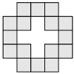
(b)

Figure 3.

⬇

Macaulay2, version 1.20

with packages: ConwayPolynomials, Elimination, IntegralClosure,

InverseSystems, Isomorphism, LLLBases, MinimalPrimes, OnlineLookup,

PrimaryDecomposition, ReesAlgebra, Saturation, TangentCone

i1 : loadPackage ”PolyominoIdeals”;

i2 : Q={{{1, 1}, {2, 2}}, {{2, 2}, {3, 3}}, {{2, 1}, {3, 2}},{{3, 2}, {4, 3}},

{{2, 3}, {3, 4}}, {{4, 1}, {5, 2}}, {{3, 4}, {4, 5}}};

i3 : I=polyoIdeal(Q);

i4 : J=polyoToric(Q,{});

i5 : R=ring I;

i6 : J=substitute(J,R);

o6 : Ideal of R

i7 : J==I

o7 = true

Consider the closed path polyomino $\mathcal{P}$ in Figure 1 (B). The polyomino ideal is not prime (see [2]), so $I_{\mathcal{P}}\subset J_{\mathcal{P}}$ since $I_{\mathcal{P}}=(J_{\mathcal{P}})_{2}$ (Lemma 3.1, [25]). We can compute also the set of the binomials generating $J_{\mathcal{P}}$ but not $I_{\mathcal{P}}$.

⬇

Macaulay2, version 1.20

with packages: ConwayPolynomials, Elimination, IntegralClosure,

InverseSystems, Isomorphism, LLLBases, MinimalPrimes, OnlineLookup,

PrimaryDecomposition, ReesAlgebra, Saturation, TangentCone

i1 : loadPackage ”PolyominoIdeals”;

i2 : Q={{{2, 1}, {3, 2}}, {{2, 2}, {3, 3}}, {{1, 2}, {2, 3}}, {{1, 3}, {2, 4}},

{{1, 4}, {2, 5}}, {{2, 4}, {3, 5}}, {{2, 5}, {3, 6}}, {{3, 5}, {4, 6}},

{{4, 5}, {5, 6}}, {{4, 4}, {5, 5}}, {{5, 4}, {6, 5}}, {{5, 3}, {6, 4}},

{{5, 2}, {6, 3}}, {{4, 2}, {5, 3}}, {{4, 1}, {5, 2}}, {{3, 1}, {4, 2}}};

i3 : I=polyoIdeal(Q);

i4 : J=polyoToric(Q,{{2,3}});

i5 : R=ring I;

i6 : J=substitute(J,R);

i7 : J==I

o7 = false

i8 : select(first entries mingens J,f->first degree f>=3)

o8 = {x x x x - x x x x }

6,5 5,1 2,6 1,2 6,2 5,6 2,1 1,5

3.4. The options Field and TermOrder

Let $\mathcal{P}$ be a collection of cells. The option Field for the function polyIdeal allows changing the base ring of the polynomial ring embedded in $I_{\mathcal{P}}$. One can choose every base ring that Macaulay2 provides. The option TermOrder allows changing the monomial order of the ambient ring of $I_{\mathcal{P}}$ as given by the function polyoIdeal. In particular, by default, it provides the lexicographic order but one can replace it with other monomial orders defined in Macaulay2. See, for instance, the following example.

⬇

Macaulay2, version 1.20

with packages: ConwayPolynomials, Elimination, IntegralClosure,

InverseSystems, Isomorphism, LLLBases, MinimalPrimes, OnlineLookup,

PrimaryDecomposition, ReesAlgebra, Saturation, TangentCone

i1 : loadPackage ”PolyominoIdeals”;

i2 : Q={{{1,1},{2,2}},{{2,2},{3,3}},{{3,3},{4,4}}};

i3 : I = polyoIdeal(Q,RingChoice=>1,TermOrder=> GRevLex);

o3 : Ideal of QQ[x , x , x , x , x , x , x , x , x , x ]

4,4 4,3 3,4 3,3 3,2 2,3 2,2 2,1 1,2 1,1

i4 : R=ring I;

i5 : describe R

o5 = QQ[x , x , x , x , x , x , x , x , x , x ,

4,4 4,3 3,4 3,3 3,2 2,3 2,2 2,1 1,2 1,1

Degrees => {10:1}, Heft => {1}, MonomialOrder => {MonomialSize => 32},

DegreeRank => 1{GRevLex => {10:1}}{Position => Up}]

3.5. RingChoice: an option for the function PolyoIdeal

Let $\mathcal{P}$ be a collection of cells. Recall that the definition of a ring in Macaulay2 needs to provide, together with a base ring and a set of variables, also a monomial order. RingChoice is an option that allows choosing between two available rings that one can define into $I_{\mathcal{P}}$.
If RingChoice is equal to 1, or by default, the function polyoIdeal gives the ideal $I_{\mathcal{P}}$ in the polynomial ring $S_{\mathcal{P}}=K[x_{a}:a\in V(\mathcal{P})]$, where $K$ is a field and the monomial order is defined by Term order induced by the following order of the variables: $x_{a}>x_{b}$ with $a=(i,j)$ and $b=(k,l)$, if $i>k$, or $i=k$ and $j>l$.
Now we describe what is the ambient ring in the case RingChoice has a value different from 1. Consider the edge ring $R=K[s_{i}t_{j}:(i,j)\in V(\mathcal{P})]$ associated to the bipartite graph $G$ with vertex set $\{s_{1},\dots,s_{m}\}\cup\{t_{1},\dots,t_{n}\}$ such that each vertex $(i,j)\in V(\mathcal{P})$ determines the edge $\{s_{i},t_{j}\}$ in $G$. Let $S=K[x_{a}:a\in V(\mathcal{P})$ and $\phi:S\rightarrow R$ be the $K$-algebra homomorphism defined by $\phi(x_{ij})=s_{i}t_{j}$, for all $(i,j)\in V(\mathcal{P})$ and set $J_{\mathcal{P}}=\ker(\phi)$. From Theorem 2.1 of [28], we know that $I_{\mathcal{P}}=J_{\mathcal{P}}$, if $\mathcal{P}$ is a weakly connected and convex collection of cells. In such a case, from [19] we get that the generators of $I_{\mathcal{P}}$ form the reduced Gröebner basis with respect to a suitable order $<$, and in particular the initial ideal $\mathrm{in}_{<}(I_{\mathcal{P}})$ is squarefree and generated in degree two. Following the proof in [19], the implemented routine provides the polynomial ring $S_{\mathcal{P}}$ with monomial order $<$.

Example 3.5.

The polyomino $\mathcal{P}$ in Figure 2 is convex. Using the options RingChoice => 2 to define $I_{\mathcal{P}}$, the ambient ring of $I_{\mathcal{P}}$ is given by PolyoRingConvex. Hence the initial ideal is squarefree in degree two.

⬇

Macaulay2, version 1.20

with packages: ConwayPolynomials, Elimination, IntegralClosure,

InverseSystems, Isomorphism, LLLBases, MinimalPrimes, OnlineLookup,

PrimaryDecomposition, ReesAlgebra, Saturation, TangentCone

i1 : loadPackage ”PolyominoIdeals”;

i2 : Q={{{1, 1}, {2, 2}}, {{2, 1}, {3, 2}}, {{3, 1}, {4, 2}}, {{2, 2}, {3, 3}},

{{3, 2}, {4, 3}}, {{2, 3}, {3, 4}}};

i3 : I=polyoIdeal(Q);

i4 : In= monomialIdeal(leadTerm(I))

o4 = monomialIdeal (x x , x x , x x , x x , x x , x x ,

2,4 3,3 3,3 4,2 2,3 4,2 2,4 3,2 2,3 3,2 4,2 1,1

—————————————————————————

x x , x x , x x , x x , x x , x x , x x ,

3,2 1,1 2,2 1,1 3,3 4,1 2,3 4,1 3,2 4,1 2,2 4,1 2,4 3,1

—————————————————————————

x x , x x )

2,3 3,1 2,2 3,1

i5 : Q={{{1, 3}, {2, 4}}, {{2, 2}, {3, 3}}, {{2, 3}, {3, 4}}, {{2, 4}, {3, 5}},

{{3, 4}, {4, 5}}, {{3, 3}, {4, 4}}, {{3, 2}, {4, 3}}, {{3, 1}, {4, 2}},

{{3, 5}, {4, 6}}, {{4, 4}, {5, 5}}, {{4, 3}, {5, 4}}, {{5, 4}, {6, 5}}};

i6 : I = polyoIdeal(Q,RingChoice=>2);

i7 : In= monomialIdeal(leadTerm(I))

o7 = monomialIdeal (x x , x x , x x , x x , x x , x x ,

4,6 3,1 4,6 3,2 4,1 3,2 3,2 2,3 4,2 2,3 4,6 3,3

—————————————————————————

x x , x x , x x , x x , x x , x x , x x ,

4,1 3,3 4,2 3,3 2,3 5,5 3,3 5,5 4,3 5,5 3,2 2,5 4,2 2,5

—————————————————————————

x x , x x , x x , x x , x x , x x , x x ,

3,3 2,5 4,3 2,5 4,6 3,5 4,1 3,5 4,2 3,5 4,3 3,5 5,3 1,4

—————————————————————————

x x , x x , x x , x x , x x , x x , x x ,

2,3 1,4 3,3 1,4 4,3 1,4 5,5 6,4 2,5 6,4 3,5 6,4 4,5 6,4

—————————————————————————

x x , x x , x x , x x , x x , x x , x x ,

2,3 5,4 3,3 5,4 4,3 5,4 2,5 5,4 3,5 5,4 4,5 5,4 3,2 2,4

—————————————————————————

x x , x x , x x , x x , x x , x x , x x ,

4,2 2,4 3,3 2,4 4,3 2,4 3,5 2,4 4,5 2,4 4,6 3,4 4,1 3,4

—————————————————————————

x x , x x , x x )

4,2 3,4 4,3 3,4 4,5 3,4

3.6. An example of computing other properties of the polyomino ideal

Considering the ideal computed by the function polyoIdeal it is possible to verify some algebraic properties and get some algebraic invariants of it by using the functions available in Macaulay2. Moreover, we can take advantage of the package Binomials.m2 [20], that is optimized for computations in binomial ideals. In the following list of commands we provide, for polyomino $\mathcal{P}$ in Figure 4, how to compute some properties of the ideal $I_{\mathcal{P}}$. In particular, we verify its primality, we check if it is radical and we compute a primary decomposition, the minimal primes (that in this case are the ideals in its primary decomposition), and the reduced Hilbert series.

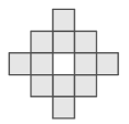
Figure 4.

⬇

Macaulay2, version 1.20

with packages: ConwayPolynomials, Elimination, IntegralClosure,

InverseSystems, Isomorphism, LLLBases, MinimalPrimes, OnlineLookup,

PrimaryDecomposition, ReesAlgebra, Saturation, TangentCone

i1 : loadPackage ”PolyominoIdeals”;

i2 : Q={{{3, 1}, {4, 2}}, {{3, 2}, {4, 3}}, {{4, 2}, {5, 3}}, {{4, 3}, {5, 4}},

{{4, 4}, {5, 5}}, {{5, 3}, {6, 4}}, {{3, 4}, {4, 5}}, {{2, 4}, {3, 5}},

{{2, 3}, {3, 4}}, {{2, 2}, {3, 3}}, {{1, 3}, {2, 4}}, {{3, 5}, {4, 6}}};

i3 : I=polyoIdeal(Q);

i4 : loadPackage ”Binomials”

i5 : binomialIsPrime(I)

o5 = false

i6 : I==binomialRadical I

Input not cellular, computing minimal primes …

o6 = true

i7 : m=binomialPrimaryDecomposition I;

i8 : #m

o8 = 4

i9 : first entries mingens m#0

o9 = {x x - x x , x x - x x , x x - x x , x x -

2,4 1,3 2,3 1,4 3,3 2,2 3,2 2,3 3,4 1,3 3,3 1,4 3,4 2,2

—————————————————————————

x x , x x - x x , x x - x x , x x - x x ,

3,2 2,4 3,4 2,3 3,3 2,4 3,5 2,2 3,2 2,5 3,5 2,3 3,3 2,5

—————————————————————————

x x - x x , x x - x x , x x - x x , x x -

3,5 2,4 3,4 2,5 4,2 3,1 4,1 3,2 4,3 2,2 4,2 2,3 4,3 3,1

—————————————————————————

x x , x x - x x , x x - x x , x x - x x ,

4,1 3,3 4,3 3,2 4,2 3,3 4,5 2,4 4,4 2,5 4,5 3,4 4,4 3,5

—————————————————————————

x x - x x , x x - x x , x x - x x , x x -

4,6 3,4 4,4 3,6 4,6 3,5 4,5 3,6 5,3 2,2 5,2 2,3 5,3 3,2

—————————————————————————

x x , x x - x x , x x - x x , x x - x x ,

5,2 3,3 5,3 4,2 5,2 4,3 5,4 4,2 5,2 4,4 5,4 4,3 5,3 4,4

—————————————————————————

x x - x x , x x - x x , x x - x x , x x -

5,5 2,4 5,4 2,5 5,5 3,4 5,4 3,5 5,5 4,2 5,2 4,5 5,5 4,3

—————————————————————————

x x , x x - x x , x x - x x , x x - x x ,

5,3 4,5 5,5 4,4 5,4 4,5 6,4 4,3 6,3 4,4 6,4 5,3 6,3 5,4

—————————————————————————

x x x x - x x x x , x x x x - x x x x ,

5,4 4,1 3,6 1,3 5,3 4,6 3,1 1,4 5,4 4,1 3,6 2,2 5,2 4,6 3,1 2,4

—————————————————————————

x x x x - x x x x , x x x x - x x x x ,

5,4 4,1 3,6 2,3 5,3 4,6 3,1 2,4 5,5 4,1 3,6 2,2 5,2 4,6 3,1 2,5

—————————————————————————

x x x x - x x x x , x x x x - x x x x ,

5,5 4,1 3,6 2,3 5,3 4,6 3,1 2,5 6,4 4,1 3,5 1,3 6,3 4,5 3,1 1,4

—————————————————————————

x x x x - x x x x , x x x x - x x x x ,

6,4 4,1 3,6 1,3 6,3 4,6 3,1 1,4 6,4 4,1 3,6 2,3 6,3 4,6 3,1 2,4

—————————————————————————

x x x x - x x x x , x x x x - x x x x ,

6,4 4,2 2,5 1,3 6,3 4,5 2,2 1,4 6,4 4,2 3,5 1,3 6,3 4,5 3,2 1,4

—————————————————————————

x x x x - x x x x , x x x x - x x x x ,

6,4 4,2 3,6 1,3 6,3 4,6 3,2 1,4 6,4 5,2 2,5 1,3 6,3 5,5 2,2 1,4

—————————————————————————

x x x x - x x x x }

6,4 5,2 3,5 1,3 6,3 5,5 3,2 1,4

i10 : first entries mingens m#1

o10 = {x , x , x , x , x , x , x , x , x x - x x ,

3,2 3,3 3,4 3,5 4,2 4,3 4,4 4,5 2,4 1,3 2,3 1,4

————————————————————————–

x x - x x , x x - x x , x x - x x ,

5,3 2,2 5,2 2,3 5,5 2,4 5,4 2,5 6,4 5,3 6,3 5,4

————————————————————————–

x x x x - x x x x }

6,4 5,2 2,5 1,3 6,3 5,5 2,2 1,4

i11 : first entries mingens m#2

o11 = {x , x , x , x , x , x , x , x , x x - x x ,

2,3 2,4 3,3 3,4 4,3 4,4 5,3 5,4 3,5 2,2 3,2 2,5

————————————————————————–

x x - x x , x x - x x , x x - x x ,

4,2 3,1 4,1 3,2 4,6 3,5 4,5 3,6 5,5 4,2 5,2 4,5

————————————————————————–

x x x x - x x x x }

5,5 4,1 3,6 2,2 5,2 4,6 3,1 2,5

i12 : first entries mingens m#3

o12 = {x , x , x , x , x , x , x , x , x , x , x , x }

2,3 2,4 3,2 3,3 3,4 3,5 4,2 4,3 4,4 4,5 5,3 5,4

i13 : n=binomialMinimalPrimes I;

i14 : n==m

o14 = true

i15 : reduceHilbert hilbertSeries I

2 3 4 5 6

1 + 12T + 50T + 92T + 76T + 24T + 2T

o15 = —————————————–

12

(1 - T)

4. A trick with the help of GeoGebra

In order to make tests for some big polyominoes or collections of cells, it could be not so easy to provide to Macaulay2 the list of the diagonal corners of each cell that encodes our object. In this section, we give a trick to obtain the encoding of a desired collection of cells, after drawing it in GeoGebra. GeoGebra is a dynamic mathematics software for all levels of education that brings together geometry, algebra, spreadsheets, graphing, statistics, and calculus in one engine. Its usage is very intuitive, in particular in the Graphics View it is possible to draw points, vectors, segments, lines, polygons, and many other things. The Graphics View Toolbar provides a wide range of Tools that allow you to create the graphical representations of objects directly in the Graphics View. GeoGebra allows to export its materials in several formats, including SVG, Animated GIF, Windows Metafile, PNG, PDF, and EPS, and can also generate code for use in LaTeXfiles. GeoGebra is available on multiple platforms, with apps for desktops (Windows, macOS and Linux), tablets (Android, iPad and Windows) and web. For many other insights see [11]. In the following explanation, we use the web app in the English(UK) language.

First of all, we explain how a collection of cells must be drawn in GeoGebra. In the Graphics View, by default, the coordinate axes and the grid appear. In the Graphics View Toolbar select the tool Regular polygon. This tool works in the following way: if one selects two points $A$ and $B$ in the plane and specifies the number $n$ of vertices in the input field of the appearing dialog window, then a regular polygon with $n$ vertices including points $A$ and $B$ is provided. We use this tool to draw each cell of the collection we want to study, as a regular polygon of $4$ vertices. For our purpose, each cell must be drawn by selecting first the lower left corner, say $A$, and then the lower right corner $A+(1,0)$, using only integer points (see Figure 5).

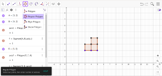
Figure 5.

In order to continue, we provide here the code of the function “GeoPoly” that we need to import in Macaualy2. If one uses a different language in GeoGebra, the code of the function must be changed opportunely.

⬇

GeoPoly=(n)->(

out={};

for i from 1 to n do (

out=join(out,{”{Vertex(poly”|i|”,1),Vertex(poly”|i|”,3)}”});

);

”vertices” << out << endl << close;

return out;

);

Now suppose the collection of cells drawn in GeoGebra has $n$ cells. In the command line of Macaulay2, type the command “GeoPoly($n$)”. This function creates the text file “vertices.txt” in the local folder where Macaulay2 is launched. So, open the file “vertices.txt” and copy and paste its content in the Input Bar of the GeoGebra window (to activate it, go to the options up-right) where the collection of cells is drawn, and type Enter (see Figure 6).

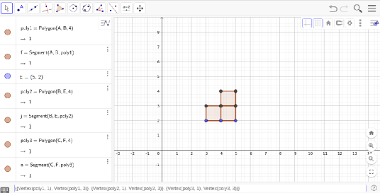
Figure 6.

In this way a list is generated, where each element is the list of the diagonal corners of each cell. Let $l1$ be the name of this list and, in the Input bar, type the command “Text(l1)” (see Figure 7).

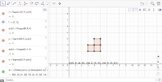
Figure 7.

Observe that, at this point, we can obtain the input data in Macaulay2 of the drawn collection of cells by the text appearing in the Graphic view. We only need to change parentheses with braces.
A possible way to obtain the character string of the text in the Graphic view, is to export it as PGF/TikZ (see Figure 8).

Figure 8.

In the exported file (that is a .txt file), one can find the desired character string in a particular line (see Figure 9 for the example explained in the previous pictures).

Figure 9.

Finally, copy the character string, open Macaulay2 and paste it into the command line creating a variable P. That is, in the command line of Macaulay2 you have something like P={{(3, 2), (4, 3)}, {(4, 2), (5, 3)}, {(4, 3), (5, 4)}} (considering the polyomino in the previous pictures). In order to replace parentheses in braces, and so obtain the right encoding of the desired collection of cells in a variable Q, it suffices to type the following commands:

⬇

Macaulay2, version 1.20

with packages: ConwayPolynomials, Elimination, IntegralClosure,

InverseSystems, Isomorphism, LLLBases, MinimalPrimes, OnlineLookup,

PrimaryDecomposition, ReesAlgebra, Saturation, TangentCone

i1 : P={{(3, 2), (4, 3)}, {(4, 2), (5, 3)}, {(4, 3), (5, 4)}};

i2 : Q={};

for i from 0 to #P-1 do(

Q=join(Q,{{toList(P#i#0),toList(P#i#1)}});

);

i4 : Q

o4 = {{{3, 2}, {4, 3}}, {{4, 2}, {5, 3}}, {{4, 3}, {5, 4}}}

o4 : List

The list Q encodes the desired collection of cells drawn in the Graphic view of GeoGebra, and from it, we are able to use the functions of the package PolyominoIdeals.m2.

References

- [1]
- [2] C. Cisto, F. Navarra, Primality of closed path polyominoes, Journal of Algebra and its Applications, Vol. 22, No. 02, 2350055, 2023.
- [3] C. Cisto, F. Navarra, R. Utano, Primality of weakly connected collections of cells and weakly closed path polyominoes, Illinois Math. Journal, 1-19, 2022.
- [4] C. Cisto, F. Navarra, R. Utano, On Gröbner bases and Cohen-Macaulay property of closed path polyominoes, The Electronic Journal of Combinatorics, 29, 3, 2022.
- [5] C. Cisto, F. Navarra, R. Utano, Hilbert-Poincaré series and Gorenstein property for closed path polyominoes, Bull. Iranian Math. Soc., 49(3): Article number 22, 2023.
- [6] C. Cisto, F. Navarra, D. Veer, Polyocollection ideals and primary decomposition of polyomino ideals, J. Algebra, 641: 498-529, 2024.
- [7] R. Dinu, F. Navarra, Non-simple polyominoes of König type, arXiv:2210.12665, preprint.
- [8] R. Dinu, F. Navarra, On the rook polynomial of grid polyominoes, arXiv:2309.01818, 2023.
- [9] V. Ene, J. Herzog, T. Hibi, Linearly related polyominoes, Journal of Algebraic Combinatorics, 41(4), 2015.
- [10] V. Ene, J. Herzog, A. A. Qureshi, F. Romeo, Regularity and Gorenstein property of the L-convex polyominoes, The Electronic Journal of Combinatorics, 28(1), P1.50, 2021.
- [11] GeoGebra.org, https://wiki.geogebra.org/en/Manual
- [12] S. W. Golomb, Polyominoes, puzzles, patterns, problems, and packagings, Second edition, Princeton University Press, 1994.
- [13] D. R. Grayson, M. E. Stillman, “Macaulay2: a software system for research in algebraic geometry”, available at http://www.math.uiuc.edu/Macaulay2.
- [14] J. Herzog, T. Hibi, Finite distributive lattices, polyominoes and ideals of König type, Internat. J. Math., 34(14): 2350089, 2023.
- [15] J. Herzog, T. Hibi, H. Ohsugi, Binomial Ideals, Graduate Texts in Mathematics, v. 279, Springer, 2018.
- [16] J. Herzog, S. S. Madani, The coordinate ring of a simple polyomino, Illinois J. Math., 58, 981–995, 2014.
- [17] J. Herzog, A. A. Qureshi, A. Shikama, Gröbner basis of balanced polyominoes, Math. Nachr., 288(7), 775–783, 2015.
- [18] T. Hibi, A. A. Qureshi, Nonsimple polyominoes and prime ideals, Illinois J. Math., 59, 391–398, 2015.
- [19] T. Hibi, H. Ohsugi, Koszul bipartite graphs, Adv. Appl. Math., 22, 25-28, 199.
- [20] T. Kahle, Decompositions of binomial ideals, J. Softw. Algebra Geom., 4 , 1–5,2 012.
- [21] M. Kummini, D. Veer, The -polynomial and the rook polynomial of some polyominoes, Electron. J. Comb., 30(2): #P2.6, 2023.
- [22] M. Kummini, D. Veer, The Charney-Davis conjecture for simple thin polyominoes, Comm. Algebra , 51(4): 1654-1662, 2022.
- [23] R. Jahangir, Hilbert Series of Polyomino Ideals and Cohen-Macaulay Posets, PhD Thesis, (2024) Sabanci University, Turkey.
- [24] R. Jahangir, F. Navarra, Shellable simplicial complex and switching rook polynomial of frame polyominoes, J. Pure Appl. Algebra, 228(6): 107576, 2024.
- [25] C. Mascia, G. Rinaldo, F. Romeo, Primality of multiply connected polyominoes, Illinois J. Math., 64(3), 291–304, 2020.
- [26] C. Mascia, G. Rinaldo, F. Romeo, Primality of polyomino ideals by quadratic Gröbner basis, Mathematische Nachrichten 295(3), 593–606, 2022.
- [27] F. Navarra, Ideals generated by the inner 2-minors of collections of cells, PhD Thesis, 2023. https://hdl.handle.net/10447/594519
- [28] A. A. Qureshi, Ideals generated by 2-minors, collections of cells and stack polyominoes, J. Algebra 357, 279–303, 2012.
- [29] A. A. Qureshi, G. Rinaldo, F. Romeo, Hilbert series of parallelogram polyominoes, Res. Math. Sci. 9(28), 2022.
- [30] A. A. Qureshi, T. Shibuta, A. Shikama, Simple polyominoes are prime, J. Commut. Algebra, 9(3), 413–422, 2017.
- [31] G. Rinaldo, and F. Romeo, Hilbert Series of simple thin polyominoes, J. Algebr. Comb. 54, 607–624, 2021.
- [32] A. Shikama, Toric representation of algebras defined by certain nonsimple polyominoes, J. Commut. Algebra, 10, 265–274, 2018.