Beyond Pairwise: Higher-order physical interactions affect phase separation in multi-component liquids
Abstract
Phase separation, crucial for spatially segregating biomolecules in cells, is well-understood in the simple case of a few components with pairwise interactions. Yet, biological cells challenge the simple picture in at least two ways: First, biomolecules, like proteins and nucleic acids, exhibit complex, higher-order interactions, where a single molecule may interact with multiple others simultaneously. Second, cells comprise a myriad of different components that form various droplets. Such multicomponent phase separation has been studied in the simple case of pairwise interactions, but an analysis of higher-order interactions is lacking. We propose such a theory and study the corresponding phase diagrams numerically. We find that interactions between three components are similar to pairwise interactions, whereas composition-dependent higher-order interactions between two components can oppose phase separation. This surprising result can only be revealed from the equilibrium phase diagrams, implying that the often-used stability analysis of homogeneous states is inadequate to study these systems. We thus show that higher-order interactions could play a crucial role in forming droplets in cells, and their manipulation could offer novel approaches to controlling multicomponent phase separation.
I Introduction
Phase separation provides a thermodynamic mechanism that partitions multicomponent liquids. The spontaneous segregation of molecules into droplets is crucial in chemical engineering and is implicated in the intricate organization of biological cells. Biological cells comprise thousands of different components that separate into various droplets known as biomolecular condensates [1], each containing hundreds of components [2]. Yet, the formation of condensates is often discussed in the simple framework of a binary Flory-Huggins theory [3, 4], which describes how two components segregate from each other because of an effective repulsive interaction [5, 6]. While this simple theory qualitatively explains phase separation of a single condensate type, it does not account for the complexity in cells. A defining feature of cells is that they are alive, so phase separation might be affected by active processes [7]. However, even the passive behavior of biomolecules in cells differs from the simplest model: First, biomolecules have complex interactions that are not captured by the Flory-Huggins free energy, and, second, there are thousands of different molecules that form multiple types of condensates simultaneously. While these challenges have been addressed separately, a combined theory describing both aspects is lacking.
The molecular interactions of biomolecules, like proteins and nucleic acids, are difficult to measure experimentally since they are generally weak and depend on the physiochemical properties of their surrounding [8]. Partial experimental measurements can be used to inform theory [9, 10, 11, 12, 13], and coarse-grained simulations can unveil sequence-based grammars to describe phase separation [14, 15, 16]. These works, and even simple polymer models [17, 18], suggest that interaction energies of biomolecules cannot be characterized by the simple quadratic terms in the Flory-Huggins theory [5, 6]. This is not surprising given the complexity of the molecules and the high volume fraction of macromolecules of about in cells [19], which together suggest that a virial expansion only up to second order is insufficient [20]. Moreover, biomolecules tend to have many different domains [21, 22], so they can interact with multiple components simultaneously. Such higher-order interactions appear naturally in colloidal systems [23, 24, 25], lead to complex competitions between components [26], enable allosteric effects [27], and explain the behavior of ternary lipid systems [28]. More broadly, higher-order interactions are vital in ecological networks [29, 30, 31, 32, 33, 34, 35, 36], and they generally emerge from coarse-graining complex interactions [37, 38]. It is thus likely that higher-order interactions are also crucial to explain the observed complex phase diagrams in cells [11].
Another complexity of cellular phase separation originates from the many different components that form multiple distinct droplets. Such multicomponent phase separation currently cannot be described adequately with detailed numerical simulations, so more abstract approaches have been developed [39]. However, even for the relatively simple Flory-Huggins theory, concrete phase diagrams are complex and can only be predicted for few components [40, 39]. Liquids with a large number of components have been studied using linear stability of the homogeneous state. For random pairwise interactions, this analysis predicts that multicomponent liquids either demix into as many phases as components, or condense into just one or two phases [41, 19, 42, 43]. Since neither behavior describes biological reality, this suggests that either linear stability analysis is inadequate or higher-order interactions are relevant in cellular phase separation.
To understand the impact of higher-order interactions on multicomponent phase separation, we study a systematically extended Flory-Huggins theory. We find that interactions that involve three different species play a similar role to pairwise interactions, whereas higher-order interactions that only involve two species, describing composition-dependent interactions, can strongly oppose normal tendencies to phase separate. Some of these qualitative differences can only be revealed from equilibrium phase diagrams, but not from the simpler linear stability analysis.
II Theory
II.1 Multicomponent mixtures with cubic interactions
We consider an incompressible, isothermal mixture of species, including one inert solvent . The composition is then described by the volume fractions of the interacting species, while the solvent fraction is . The thermodynamics of the system are governed by the free energy density
| (1) |
where is the relevant energy scale, and denotes a molecular volume, which we consider to be the same for all species for simplicity. The terms on the first line capture the translational entropy of all species, while all other contributions to the energy are described by the terms in the second line. The second line can be interpreted as a Taylor expansion in terms of the densities . The lowest orders of the expansion do not contribute since the zeroth-order term just shifts the overall energy and terms linear in drop out in the equilibrium conditions; see below. The first relevant term is the quadratic one, which quantifies the principle pair interactions between species and by Flory parameters ; positive values denote effective repulsion of species and , whereas negative values lead to attraction [5, 6]. Finally, the last term in Eq. 1 quantifies cubic interactions among species , , and by a parameter , which we address in this paper. Terms of higher order could be included (see Appendix for a general framework), but we limit the discussion to third-order interactions for simplicity. The sums in Eq. 1 imply that only the symmetric parts of the interaction parameters contribute, so we can assume and . Moreover, we exploit incompressibility (), and the fact that terms linear in do not change the equilibrium states, to remove diagonal entries (). The thermodynamics of the liquid are then fully described by the two sets of interaction parameters and .
The cubic interactions quantified by describe two fundamentally different physical processes. To see this, we rewrite the second line in Eq. 1 as by introducing re-scaled pair interactions
| (2) |
which now depend on the composition . The first term on the right hand side summarizes the familiar quadratic interactions, but we split the cubic interactions into two fundamentally different contributions: The last term captures true cubic interactions between three different species (), which we thus call ternary cubic interactions. In contrast, the middle term describes composition-dependent pair interactions, where the coefficients and capture how the pair-interaction depends on the composition of the two involved species, and we thus call these binary cubic interactions. Such composition-dependent pair interactions are often used for describing real polymers [44].
In a system with components (including the inert solvent), the interaction parameters and have and independent entries, respectively. To limit this large parameter space, we for simplicity only consider random interaction matrices, where the entries of and are drawn independently from normal distributions. Specifically, we chose the quadratic interactions as , the binary cubic interactions as , and the ternary cubic interactions as , where represents a normal distribution with mean and variance . Our model is thus parametrized by the component count and six parameters describing the distributions of the interaction parameters.
II.2 Unstable modes of homogeneous states
One approach to investigate the behavior of multicomponent liquids is to analyze homogeneous states, which are quantified by the volume fractions . Such a state is stable if the Hessian of the free energy,
| (3) |
is positive definite, i.e., if all its eigenvalues are positive. In contrast, the homogeneous state is unstable if one of the eigenvalues is negative, indicating that the system would split into different phases. We expect that the number of unstable modes , i.e., the number of negative eigenvalues, is correlated with the number of distinct phases that form during phase separation. For instance, the homogeneous state must be stable when it is the only stable state ( implies ). Moreover, we expect the maximal number of phases () when all modes are unstable (). Taken together, the simplest hypothesis for the correlation is thus , but since the eigenvalue analysis strictly only applies to infinitesimal small deviations from the homogeneous phase, it is unclear how well predicts fully phase separated states. To investigate this in detail, we thus also quantify coexisting phases directly.
II.3 Phase count in equilibrium states
Coexisting phases need to obey thermodynamic conditions, enforcing equal chemical potentials and pressures in all phases [7]. Denoting the volume fraction of the -th species in the -th phase by , we express these intensive quantities in non-dimensional form, and , implying
| (4a) | ||||
| (4b) | ||||
The coexistence conditions thus read
| and | (5) |
for and . These are independent conditions, which need to be satisfied for phases to coexist. These non-linear equations are difficult to solve explicitly and we thus resort to a numerical Monte-Carlo method [45] to discover solutions. Since the original implementation weighted compositions with similar fractions much more heavily [46], we have improved the method to find a solution of these equations for a given average fraction. Briefly, we initialize many compartments with random compositions such that the composition averaged over all compartments assumes a desired value. We then minimize the overall free energy by exchanging components and volume between compartments until a stationary state is reached, which corresponds to thermodynamic equilibrium [45]. We can then analyze the coexisting equilibrium phases and uniformly sample the phase space.
III Results
To analyze the impact of cubic interactions on phase separation, we will first investigate the simpler situation of few components with symmetric interactions. After increasing the component count in the third subsection, we will finally study the impact of diverse cubic interactions.
III.1 Attractive binary cubic interactions promote phase separation
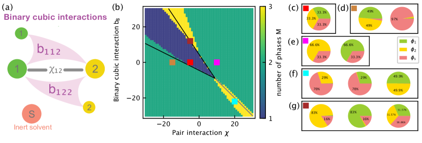
We first focus on the effect of the binary cubic interactions in the simplest system with components; see Fig. 1(a). Since the solvent is inert, only two species interact with each other and the ternary cubic interaction does not contribute. For simplicity, we first consider identical interactions ( and ) and equal fractions of all components (). Fig. 1(b) reveals that the system exhibits either one or two phases without cubic interactions (). The former case corresponds to a stable homogeneous state, see Fig. 1(c), whereas the latter comes in two flavors: For strong attraction (), species and are equally enriched in one phase and together segregate from the solvent; see Fig. 1(d). In contrast, for strong repulsion (), species and separate from each other with equal solvent fractions throughout; see Fig. 1(e). Binary cubic interactions () significantly impact the phase diagram, revealing unexpected regions supporting three phases (yellow areas in Fig. 1(b)). We again observe two qualitatively different regions: For negative and positive , the two solutes form one phase with barely any solvent, whereas the other two phases exhibit a lot of solvent and either one of the solutes; see Fig. 1(f). Conversely, for positive and negative , each solute dominates in one phase, whereas the third phase has a balanced composition of all components; see Fig. 1(g). Notably, when , marked by the gray line in Fig. 1(b), all three species behave equivalently, so the system necessarily forms three phases when the interactions are sufficiently repulsive. The apparent interaction of the solutes with the inert solvent is a consequence of incompressibility; see Appendix. This particular case also reveals that the effect of binary cubic interactions can at least partly be described by effective interactions with the inert solvent. This initial investigation shows that binary cubic interactions affect what phases coexist when they oppose the binary quadratic interactions .
To analyze the effect of binary cubic interactions on the three-component system further, we next investigate the phase diagrams as a function of compositions at fixed and . Fig. 2(a) shows the phase count averaged over all possible compositions. Most of the phase diagram exhibits roughly two phases, but the homogeneous state dominates in a part of the upper left quadrant; similar to Fig. 1(b). Interestingly, the two parameter regions that exhibited three phases for equal composition (see Fig. 1(b)) are now less prominent. To analyze the effect of the cubic interactions more clearly, we average over all values of ; see right panel in Fig. 2(a). This quantification reveals that attractive binary cubic interactions () increase the average phase count and thus promote phase separation, whereas repulsive interactions tend to suppress phase separation unless they are very strong. A similar result is also visible in the quantification of the number of unstable modes shown in Fig. 2(b), although the direct comparison between and shown in Fig. 2(c) reveals that often deviates substantially from .
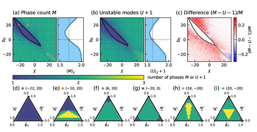
To understand the role of composition in more detail, we next determine the full phase diagrams for particular choices of ; see Fig. 2(d–i). For large positive , the homogenous phase is the only stable phase when (Fig. 2(d)), indicating that repulsive binary cubic interactions can suppress phase separation. However, slightly larger values of can lead to rich phase diagrams, also involving three-phase regions (Fig. 2(e)), until the two-phase region dominates for positive (Fig. 2(f)). Here, the homogeneous system is only favored when the solvent fraction is very high. Conversely, the homogeneous state is favored for low when the cubic interactions are absent; see Fig. 2(g). When the binary cubic interactions are attractive (), the homogenous state is rare and we again find three-phase regions; see Fig. 2(h). Interestingly, the width of the three-phase region becomes smaller for small , whereas it became wider in Fig. 2(e), which might be caused by the opposite signs of the interactions in these two cases. Moreover, Fig. 2(i) reveals that the special case of indeed leads to symmetric interactions between all species. stinct roles played by binary cubic attraction and repulsion.
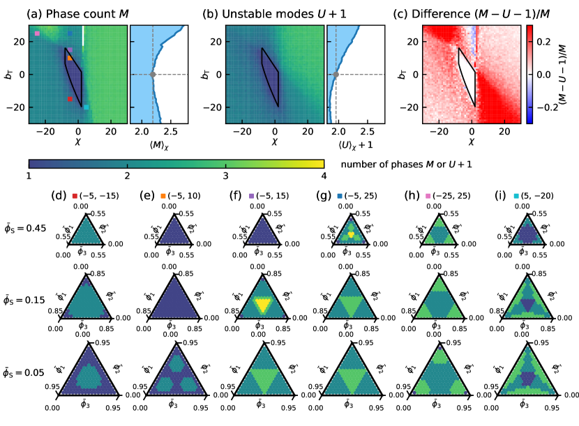
The influence of binary cubic interactions can be partly rationalized by interpreting them as effective pair interactions. For and , Eq. 2 reduces to , implying that repulsive cubic interactions () generally increase . This equation also reveals that the sum of the parameters and is crucial, explaining why interesting phase emerge in the region where is small. The effect on is particularly large when the fraction of the inert solvent is low, explaining why we find more phases in the lower part of Fig. 2(e). Conversely, for attractive cubic interactions (), we find in the special case , showing that the effective interaction becomes more repulsive for larger solvent fraction , consistent with Fig. 2(h). Taken together, this analysis again reveals that binary cubic interactions can partly be interpreted as interactions with the inert solvent. In particular, repulsive binary cubic interactions stabilize homogeneous states, whereas attractive interactions promote phase separation.
III.2 Repulsive ternary cubic interactions promote phase separation
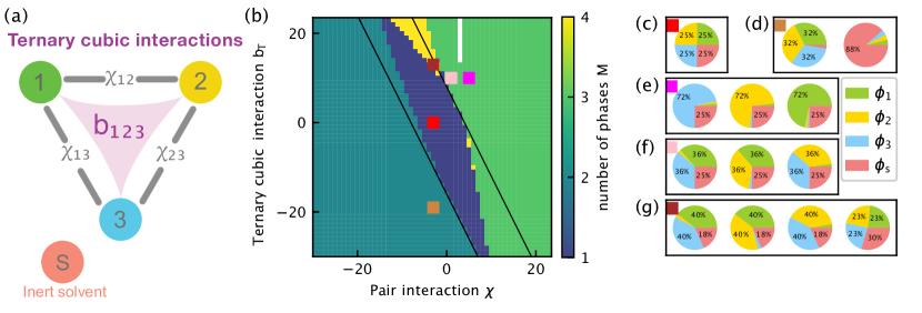
We next analyze the effect of ternary cubic interactions that characterize the interplay among three different species in a liquid with components; see Fig. 3(a). We start by considering identical interactions across all species (vanishing variances; ) without binary cubic interactions () for equal fractions (), so the only two control parameters are and . Fig. 3(b) shows the system exhibits between one and three phases without ternary cubic interactions (). In particular, only the homogeneous state is stable for weak binary interactions (small ); see Fig. 3(c). Strong attraction () results in a phase enriched in species , , and , which together segregate from the inert solvent, and hence form two phases whose compositions are similar to that shown in Fig. 3(d). In contrast, for strong repulsion (), species , , and separate from each other with equal solvent fractions throughout, leading to three phases with compositions similar to those shown in Fig. 3(e). Adding ternary cubic interactions () enriches the phase diagram: In particular, we now find one parameter region supporting four phases when ternary cubic interactions are repulsive (, but ); see yellow area in Fig. 3(b). Surprisingly, two solute components co-segregate together in three of the phases, whereas the solvent dominates the fourth one; see Fig. 3(g). The detailed compositions also reveal additional transitions in regions where panel b reports the same phase count. For instance, in the large bright green region (), we observe a transition from three phases where always two solutes co-segregate (Fig. 3(f), ) to three phases that are each dominated by a single solute (Fig. 3(e), ). Taken together, this initial analysis suggests ternary cubic interactions result in interesting phases, which cannot be explained by a simple re-scaling of quadratic interactions.
To analyze the effect of composition, we next investigate the phase count averaged over all compositions. The features of the respective diagram shown in Fig. 4(a) are similar to Fig. 3(b); Attractive quadratic interactions () generally lead to two phases, whereas strong repulsion () leads to three phases. Weak interactions stabilize the homogeneous state, although the parameter region where this is the only possible state (enclosed by the black line) is smaller than in Fig. 3(b). Adding ternary cubic interactions has qualitatively similar effects to the case of equal composition shown in Fig. 3(b): Repulsive interactions () generally increase the phase count , which is particularly obvious when is averaged over all ; see right panel of Fig. 4(a). Although the number of unstable modes shown in Fig. 4(b) paints a similar picture, the predicted effects are much weaker. Moreover, Fig. 4(c) reveals that consistently underestimates , particularly when ternary cubic interactions oppose quadratic interactions. Taken together, this suggests that repulsive ternary cubic interactions promote phase separation, similar to repulsive quadratic interactions, and in stark contrast to binary cubic interactions.
To understand the role of composition in detail, we next determine the full phase diagram for particular choices of , , and ; see Fig. 4(d–i). Panel (d) reveals that attractive interactions ( and ) generally favor two phases, particularly for larger solvent fractions (upper row). In contrast, larger hinders the formation of two phases for repulsive ternary cubic interactions (large , Fig. 4(e)). Even stronger ternary repulsion can facilitate states with four phases (yellow regions in Fig. 4(f)), but both low and high suppresses this state. For large positive at low , three-phase regions appear for equal composition (bright green regions in lower panel of Fig. 4(g)), while they appear in the corner of the phase diagram when is lower; see Fig. 4(h). Finally, Fig. 4(i) shows that for positive , increasing leads to fewer phases, similar to Fig. 4(e), but now three phases can be prevalent. Taken together, these detailed phase diagrams demonstrate a profound effect of ternary interactions on the actual phases that form for a particular composition of the system.
We demonstrated that ternary cubic interactions affect the number of phases and particularly their composition. Linear stability analysis predicts this behavior even worse than in the case of binary interactions; compare Fig. 4(c) to Fig. 2(c). Although Eq. 2 demonstrates that can be interpreted as composition-dependent pairwise interactions, our numerical results indicate that third-order interactions do not merely rescale the two-body interaction . Moreover, binary cubic interactions tend to lead to more phases when they are attractive (), whereas repulsive ternary cubic interactions () tend to increase it. Taken together, even the simplest cases of and components, respectively, highlight that cubic interactions play a nontrivial role.
III.3 Ternary cubic interactions dominate binary cubic interactions in case of many components
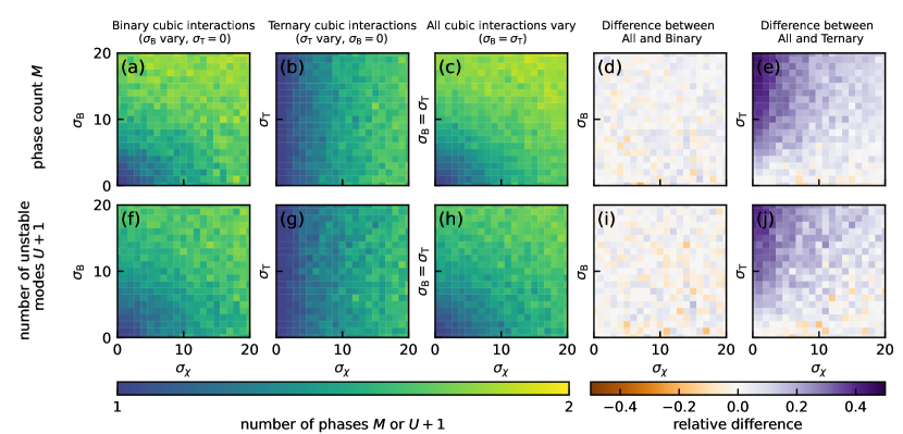
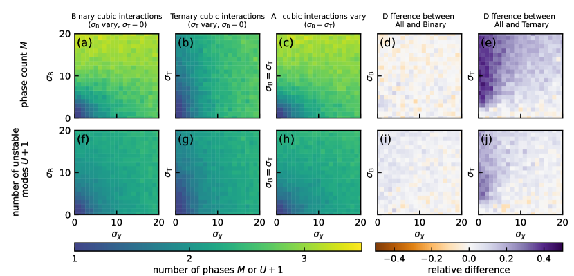
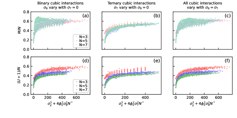
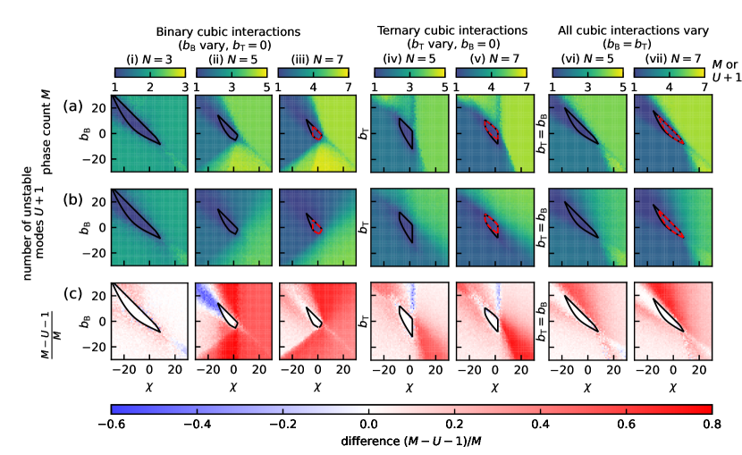
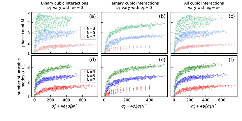
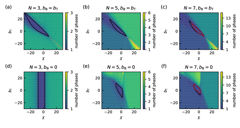
To elucidate how cubic interactions affect phases in liquids with more components, we next vary the component count . If we again used identical interactions between components, we would often find states with more than phases, seemingly violating Gibb’s phase rule [47]. This exceptional result is a consequence of the symmetry in the interaction matrix leading to degenerate states; for example, if there are states that enrich two of the interacting components (e.g., see Fig. 3f), there are choices of the component pair, all leading to states of equal energy, which can coexist. To avoid this problem and study the generic behavior where at most phases form, we thus investigate systems with almost equal interaction by setting a finite standard deviation for the interaction matrices (). Fig. 5 summarizes the results for three different cases, where binary cubic interactions vary without ternary cubic interactions (, left columns), ternary cubic interactions vary without binary cubic interactions (, middle columns), and all cubic interactions exist with identical mean (, , right columns).
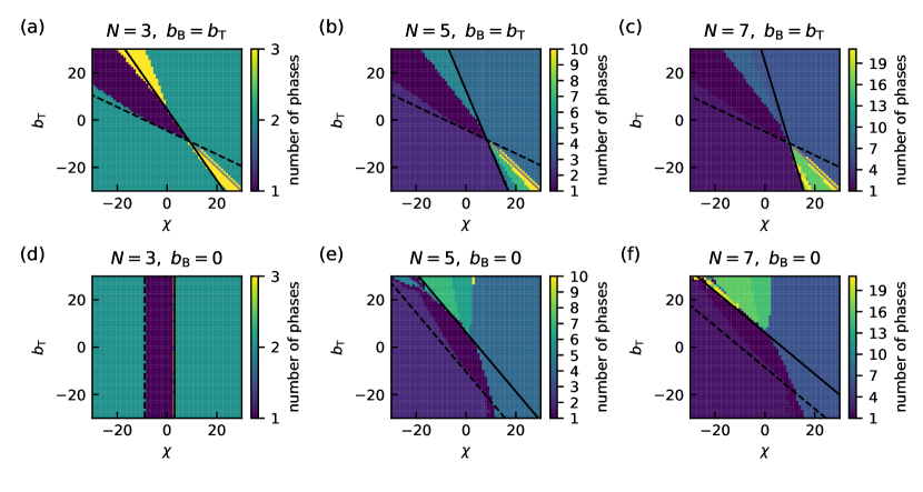
The phase count shown in the upper row of Fig. 5 indicates that there is a finite region in parameter space where the homogeneous state is stable and phase separation is impossible for all choices of and in all three scenarios. This region generally shrinks for larger , indicating that adding components promotes phase separation. However, the region stays finite even in the limit of , so that the homogeneous state is always stable for weakly interacting systems; see red dashed line in Fig. 5(a)(iii, v, vii) and Appendix. We also observe that the maximal phase count increases with , in accordance with Gibb’s phase rule. Generally, more phases () are expected when binary interactions are sufficiently repulsive (), whereas two phases form for sufficiently attractive binary interactions. While this general trend is expected [45], the cubic interactions modify the picture substantially.
The most significant difference between the three scenarios shows in the dependence of the phase count on the strength of the cubic interaction; see Fig. 5(a). Consistent with the first result section, we find that attractive binary cubic interactions () increase , particularly for large (left columns). In contrast, ternary cubic interactions tend to increase when they are repulsive (, middle columns). Interestingly, the joint scenario where both cubic interactions are present seems to be dominated by the ternary interactions since the data shown in the right columns of Fig. 5(a) resembles the data in the middle columns. However, this conclusion does not seem justified when considering the region without phase separation (enclosed by black lines), which is largest in the joint scenario. Taken together, this suggests that ternary cubic interactions dominate the phase behavior over binary cubic interactions.
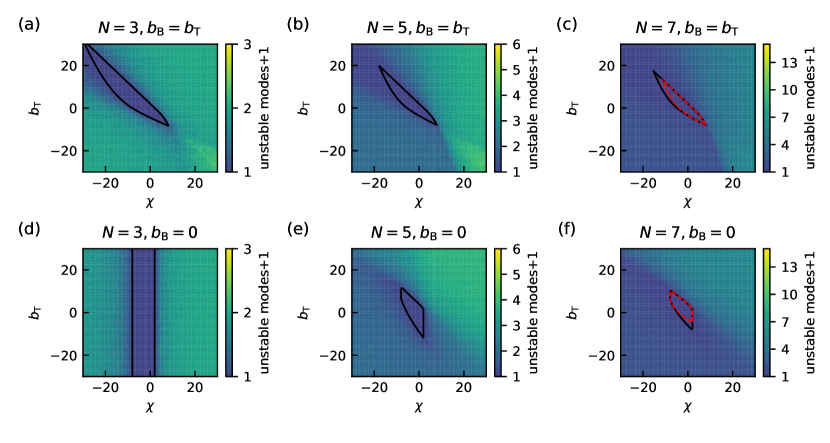
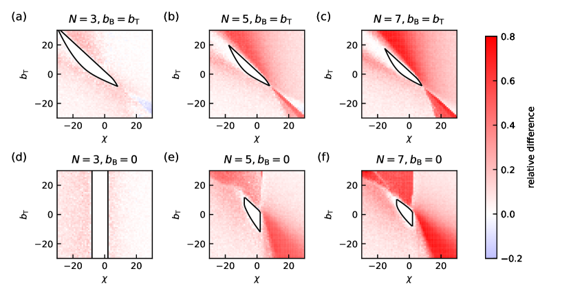
We next check whether the same conclusions could have been obtained from observing the number of unstable modes of the homogeneous state. The density plots shown in Fig. 5(b) roughly resemble the diagrams in the upper row and particularly capture the increased phase count for larger quadratic interactions . However, the influence of the cubic interactions is not even captured qualitatively. For instance, repulsive binary cubic interactions (, left columns) tend to slightly increase the phase count , whereas the number of unstable modes decreases. Similarly, the effect of attractive ternary cubic interactions (, middle columns) is not captured very well. These differences are revealed more prominently in the direct comparison shown in Fig. 5(c). This plot reveals that almost always underestimates by a significant fraction and that this discrepancy tends to increase for larger component counts . Interestingly, the disagreement seems to be less severe when both ternary interactions are considered (right column).
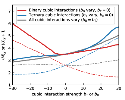
To map out the average influence of cubic interactions, we next average the measured phase counts and number of unstable modes over the analyze range of quadratic interaction parameters . Fig. 6 summarizes that cubic interactions have a strong influence on both and , and that generally underestimates significantly. This presentation also highlights that repulsive ternary cubic interactions () generally promote phase separation, whereas repulsive binary cubic interactions () increase only weakly. In contrast, attractive binary cubic interactions () increase more strongly than any other scenario, whereas attractive ternary cubic interactions () even decrease . Moreover, Fig. 6 shows that the combined scenario, where both types of cubic interactions have equal strength, is dominated by the ternary cubic interactions, presumably because it contributes more terms to the free energy; see Eq. 2. This is particularly surprising for attractive interactions, where the phase count of combined scenario lies below either of the individual cases, whereas the number of unstable modes lies between these cases. Taken together, this quantification highlights that cubic interactions have a strong effect, which is effectively opposite for binary and ternary cubic interaction. However, we have so far only considered cases where the interactions between components were relatively similar (small variance), but realistic interactions might vary widely.
III.4 Variance of binary cubic interactions raises phase count more than variance of ternary interactions
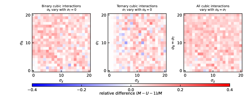
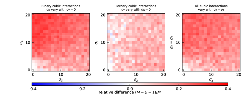
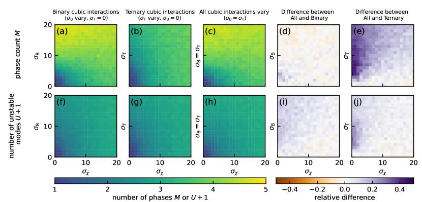
To study the role of diverse interactions, we next vary the variances , , and of the random interaction matrices, but we consider vanishing mean interactions () for simplicity. Fig. 7 shows that the average phase count always increases for larger variance of the pairwise interactions, consistent with literature [45, 43]. Similarly, increases when the variance of binary cubic interactions, of ternary cubic interactions, or both are increased. However, while large values of lead to roughly phases [43], large values of , but not , can apparently induce many more phases, consistent with the important role of binary cubic interactions revealed in the previous sections.
The combined scenario shown in Fig. 7(c) reveals that the variance of binary cubic interactions dominates the phase count, which is particularly visible in the direct comparisons shown in panels (d) and (e). This difference might originate from the strong influence of attractive binary cubic interactions, see Fig. 6, which will occur frequently in random interactions with vanishing mean. Interestingly, the difference we observe when analyzing is not visible if we instead quantify the number of unstable modes. The data shown in panels (f)–(j) again emphasizes that linear stability analysis is not well suited for predicting phase counts. Taken together, our data suggests that the variance of binary cubic interactions is more crucial than that of ternary interactions, whereas we found the opposite trend when analyzing the mean interactions in the previous section.
The phase count and the number of unstable modes shown in Fig. 7 suggest a simple dependence on the variances and . Indeed, Eq. 2 indicates that cubic interactions can be absorbed into effective pairwise interactions when analyzing the symmetric homogeneous state where ; see Appendix. The pairwise interactions of this reduced system are then a random matrix with zero mean and variance , where quantifies the number of terms that stem from cubic interaction ( for , for , and for ). This reduction suggests that systems with the same effective variance should exhibit similar behavior. Indeed, Figs. 8(d–f) show that all values collapse on a line for various when plotted as a function of . Such a collapse is also visible for the phase count for solely ternary cubic interactions Fig. 8(b). In contrast, does not collapse in systems with binary cubic interactions, and the spread even increase for larger ; see panels (a) and (c). These results are consistent with the previous finding that cubic interactions matter more when binary cubic terms are present.
We also briefly tested whether the dependence on the component count can be captured by rescaling and with . Fig. S13 in the Appendix indicates that the phase count generally scales with , whereas the number of unstable modes does less so. Since these deviations become significant at large component count (), the phase count might also show deviations for larger , which is unfortunately intractable numerically. Taken together, this analysis demonstrates that random cubic interactions can be described by re-scaled pairwise interactions when only the stability of the homogeneous state is considered. In contrast, they need to be included explicitly to describe coexisting phases, particularly when binary cubic interactions are present.
We systematically investigated the role of higher-order interactions in multicomponent phase separation. Our results demonstrate that cubic interactions influence phase separation significantly by altering the number of phases that coexist and their composition. By analyzing the coexisting phases in equilibrium, and not just the number of unstable modes of the homogeneous state, we showed that cubic interactions do not merely rescale binary interactions, which was previously suggested for random interactions [19]. Moreover, we clearly identified two distinct classes of cubic interactions: Cubic interactions between three distinct species tend to have a similar effect to binary interactions, although they can lead to more phases even when the solvent is inert. In contrast, cubic interactions between only two species, which can be interpreted as composition-dependent binary interactions, have profoundly different influences: Here, attractive interactions tend to increase the number of phases (whereas increasing the phase count otherwise would typically require repulsion). This effect is so strong that it dominates the phase count for random matrices with vanishing mean interactions, which is a case that is often studied. Taken together, we have shown that cubic interactions have profound effects and that there are different classes, which need to be treated separately. These conclusions are similar to the effect of higher-order interactions in ecology [35] and will likely translate to quartic interactions and beyond.
Our comparison of the actual phase count in equilibrium to the predictions from a linear stability of the homogeneous state suggests that the latter systematically underestimates the phase count. The predicted values can deviate by more than and becomes often worse when cubic interactions are significant. This suggests that linear stability analysis is not very suitable to analyze the phase behavior, particular in complex situations.
Higher-order interactions emerge naturally in complex systems, particularly in biological phase separation. The interaction parameters, quantified by , can in principle be calculated rigorously from first principles and validated through simulations [20, 23, 14, 16]. Alternatively, they could be determined by comparison with multi-component phase diagrams, like those presented in [12, 11]. Our work focused on random interactions to keep the number of independent parameters manageable, but it is unclear whether random interactions represent realistic systems faithfully since designed interactions provide a more diverse behavior [48, 49], and evolutionary optimization can for instance tune the condensate count [45]. Moreover, allostery could be used to engineer specific cubic interactions [27]. The resulting complex phase diagrams provide many phase boundaries, which could be used to respond to external changes in biological contexts. In this case, the precise composition of the system will affect what phases form [50]. Higher-order interactions expand the range of possibilities of such biological computations, and might thus facilitate the retrieval of target structures in multicomponent liquids [51]. These properties reminiscent of information processing might explain why phase separation is ubiquitous in biology.
acknowledgement
We thank Pablo Sartori, Izaak Neri, and Sonali Priyadarshini Nayak for helpful discussions and critical reading of the manuscript. CL thanks Baoshuang Shang and Yuanchao Hu for helpful discussions. We gratefully acknowledge funding from the Max Planck Society and the European Union (ERC, EmulSim, 101044662).
References
- Banani et al. [2017] S. F. Banani, H. O. Lee, A. A. Hyman, and M. K. Rosen, Biomolecular condensates: organizers of cellular biochemistry, Nature reviews Molecular cell biology 18, 285 (2017).
- Youn et al. [2019] J.-Y. Youn, B. J. Dyakov, J. Zhang, J. D. Knight, R. M. Vernon, J. D. Forman-Kay, and A.-C. Gingras, Properties of stress granule and p-body proteomes, Mol. Cell 76, 286 (2019).
- Hyman et al. [2014] A. A. Hyman, C. A. Weber, and F. Jülicher, Liquid-liquid phase separation in biology, Annu. Rev. Cell Dev. Biol. 30, 39 (2014).
- Jülicher and Weber [2023] F. Jülicher and C. A. Weber, Droplet physics and intracellular phase separation, Annual Review of Condensed Matter Physics 15 (2023).
- Flory [1942] P. I. Flory, Thermodynamics of high polymer solutions, The Journal of Chemical Physics, J. Chem. Phys. 10, 51 (1942).
- Huggins [1941] M. L. Huggins, Solutions of long chain compounds, The Journal of chemical physics 9, 440 (1941).
- Zwicker [2022] D. Zwicker, The intertwined physics of active chemical reactions and phase separation, Current Opinion in Colloid & Interface Science , 101606 (2022).
- Dignon et al. [2020] G. L. Dignon, R. B. Best, and J. Mittal, Biomolecular phase separation: from molecular driving forces to macroscopic properties, Annual review of physical chemistry 71, 53 (2020).
- Doi [1996] M. Doi, Introduction to polymer physics (Oxford university press, 1996).
- Fredrickson [2006] G. Fredrickson, The equilibrium theory of inhomogeneous polymers, 134 (Oxford University Press, 2006).
- Riback et al. [2020] J. A. Riback, L. Zhu, M. C. Ferrolino, M. Tolbert, D. M. Mitrea, D. W. Sanders, M.-T. Wei, R. W. Kriwacki, and C. P. Brangwynne, Composition-dependent thermodynamics of intracellular phase separation, Nature 581, 209 (2020).
- Arter et al. [2022] W. E. Arter, R. Qi, N. A. Erkamp, G. Krainer, K. Didi, T. J. Welsh, J. Acker, J. Nixon-Abell, S. Qamar, J. Guillén-Boixet, et al., Biomolecular condensate phase diagrams with a combinatorial microdroplet platform, Nature Communications 13, 7845 (2022).
- Saar et al. [2023] K. L. Saar, D. Qian, L. L. Good, A. S. Morgunov, R. Collepardo-Guevara, R. B. Best, and T. P. Knowles, Theoretical and data-driven approaches for biomolecular condensates, Chemical Reviews (2023).
- Holehouse and Kragelund [2023] A. S. Holehouse and B. B. Kragelund, The molecular basis for cellular function of intrinsically disordered protein regions, Nature Reviews Molecular Cell Biology , 1 (2023).
- Lin et al. [2018] Y.-H. Lin, J. D. Forman-Kay, and H. S. Chan, Theories for sequence-dependent phase behaviors of biomolecular condensates, Biochemistry 57, 2499 (2018).
- Pappu et al. [2023] R. V. Pappu, S. R. Cohen, F. Dar, M. Farag, and M. Kar, Phase transitions of associative biomacromolecules, Chemical Reviews (2023).
- Dudowicz et al. [2002] J. Dudowicz, K. F. Freed, and J. F. Douglas, Beyond Flory-Huggins Theory: New Classes of Blend Miscibility Associated with Monomer Structural Asymmetry, Physical Review Letters 88, 095503 (2002).
- Pesci and Freed [1989] A. I. Pesci and K. F. Freed, Lattice theory of polymer blends and liquid mixtures: Beyond the Flory–Huggins approximation, The Journal of Chemical Physics 90, 2017 (1989).
- Sear [2005] R. P. Sear, The cytoplasm of living cells: a functional mixture of thousands of components, Journal of Physics: Condensed Matter 17, S3587 (2005).
- Bruns [1997] W. Bruns, The third osmotic virial coefficient of polymer solutions, Macromolecules 30, 4429 (1997).
- Choi et al. [2020] J.-M. Choi, A. S. Holehouse, and R. V. Pappu, Physical principles underlying the complex biology of intracellular phase transitions, Annual review of biophysics 49, 107 (2020).
- [22] P. Mohanty, A. Rizuan, Y. C. Kim, N. L. Fawzi, and J. Mittal, A complex network of interdomain interactions underlies the conformational ensemble of monomeric tdp-43 and modulates its phase behavior, Protein Science , e4891.
- Russ et al. [2002] C. Russ, H. Von Grünberg, M. Dijkstra, and R. van Roij, Three-body forces between charged colloidal particles, Physical Review E 66, 011402 (2002).
- Brunner et al. [2004] M. Brunner, J. Dobnikar, H.-H. von Grünberg, and C. Bechinger, Direct measurement of three-body interactions amongst charged colloids, Physical review letters 92, 078301 (2004).
- Dobnikar et al. [2004] J. Dobnikar, M. Brunner, H.-H. von Grünberg, and C. Bechinger, Three-body interactions in colloidal systems, Physical Review E 69, 031402 (2004).
- Sanders et al. [2020] D. W. Sanders, N. Kedersha, D. S. Lee, A. R. Strom, V. Drake, J. A. Riback, D. Bracha, J. M. Eeftens, A. Iwanicki, A. Wang, et al., Competing protein-rna interaction networks control multiphase intracellular organization, Cell 181, 306 (2020).
- McCullagh et al. [2024] M. McCullagh, T. N. Zeczycki, C. S. Kariyawasam, C. L. Durie, K. Halkidis, N. C. Fitzkee, J. M. Holt, and A. W. Fenton, What is allosteric regulation? exploring the exceptions that prove the rule!, Journal of Biological Chemistry , 105672 (2024).
- Idema et al. [2009] T. Idema, J. Van Leeuwen, and C. Storm, Phase coexistence and line tension in ternary lipid systems, Physical Review E 80, 041924 (2009).
- Billick and Case [1994] I. Billick and T. J. Case, Higher order interactions in ecological communities: what are they and how can they be detected?, Ecology 75, 1529 (1994).
- Mayfield and Stouffer [2017] M. M. Mayfield and D. B. Stouffer, Higher-order interactions capture unexplained complexity in diverse communities, Nature ecology & evolution 1, 0062 (2017).
- Battiston et al. [2020] F. Battiston, G. Cencetti, I. Iacopini, V. Latora, M. Lucas, A. Patania, J.-G. Young, and G. Petri, Networks beyond pairwise interactions: Structure and dynamics, Physics Reports 874, 1 (2020).
- Grilli et al. [2017] J. Grilli, G. Barabás, M. J. Michalska-Smith, and S. Allesina, Higher-order interactions stabilize dynamics in competitive network models, Nature 548, 210 (2017).
- Bairey et al. [2016] E. Bairey, E. D. Kelsic, and R. Kishony, High-order species interactions shape ecosystem diversity, Nature communications 7, 12285 (2016).
- Gibbs et al. [2022] T. Gibbs, S. A. Levin, and J. M. Levine, Coexistence in diverse communities with higher-order interactions, Proceedings of the National Academy of Sciences 119, e2205063119 (2022).
- Kleinhesselink et al. [2022] A. R. Kleinhesselink, N. J. Kraft, S. W. Pacala, and J. M. Levine, Detecting and interpreting higher-order interactions in ecological communities, Ecology letters 25, 1604 (2022).
- Li et al. [2020] Y. Li, J. Xiao, H. Liu, Y. Wang, and C. Chu, Advances in higher-order interactions between organisms, Biodiversity Science 28, 1333 (2020).
- Thibeault et al. [2024] V. Thibeault, A. Allard, and P. Desrosiers, The low-rank hypothesis of complex systems, Nature Physics , 1 (2024).
- Herron et al. [2023] L. Herron, P. Sartori, and B. Xue, Robust retrieval of dynamic sequences through interaction modulation, PRX Life 1, 023012 (2023).
- Jacobs [2023a] W. M. Jacobs, Theory and simulation of multiphase coexistence in biomolecular mixtures, Journal of Chemical Theory and Computation (2023a).
- Mao et al. [2018] S. Mao, D. Kuldinow, M. Haataja, and A. Kosmrlj, Phase behavior and morphology of multicomponent liquid mixtures, Soft Matter 15, 1297 (2018).
- Sear and Cuesta [2003] R. P. Sear and J. Cuesta, Instabilities in complex mixtures with a large number of components., Physical Review Letters, Phys. Rev. Lett. 91, 245701 (2003).
- Jacobs and Frenkel [2017] W. M. Jacobs and D. Frenkel, Phase transitions in biological systems with many components, Biophys. J. 112, 683 (2017).
- Shrinivas and Brenner [2021] K. Shrinivas and M. P. Brenner, Phase separation in fluids with many interacting components, Proc. Natl. Acad. Sci. USA 118, 10.1073/pnas.2108551118 (2021).
- Baulin and Halperin [2002] V. Baulin and A. Halperin, Concentration dependence of the flory parameter within two-state models, Macromolecules 35, 6432 (2002).
- Zwicker and Laan [2022] D. Zwicker and L. Laan, Evolved interactions stabilize many coexisting phases in multicomponent liquids, Proceedings of the National Academy of Sciences 119, e2201250119 (2022).
- Jacobs [2023b] W. M. Jacobs, Theory and simulation of multiphase coexistence in biomolecular mixtures, J. Chem. Theory Comput. 19, 3429 (2023b).
- Gibbs [1876] J. W. Gibbs, On the equilibrium of heterogeneous substances, Transactions of the Connecticut Academy of Arts and Sciences, Trans. Conn. Acad. Arts Sci. 3, 1 (1876).
- Mao et al. [2019] S. Mao, D. Kuldinow, M. P. Haataja, and A. Košmrlj, Phase behavior and morphology of multicomponent liquid mixtures, Soft Matter 15, 1297 (2019).
- Chen and Jacobs [2023] F. Chen and W. M. Jacobs, Programmable phase behavior in fluids with designable interactions, The Journal of Chemical Physics 158 (2023).
- Thewes et al. [2023] F. C. Thewes, M. Krüger, and P. Sollich, Composition dependent instabilities in mixtures with many components, Physical Review Letters 131, 058401 (2023).
- Teixeira et al. [2023] R. B. Teixeira, G. Carugno, I. Neri, and P. Sartori, Liquid hopfield model: retrieval and localization in heterogeneous liquid mixtures, arxiv 2310.18853 (2023).
Appendix A Theory for multi-component mixtures with higher-order interactions
We first write the free energy for the incompressible component mixtures with internal energies for species , pair interactions between species and , and higher-order interactions. We denote the -order interaction among species as , and include interactions up to order . The free energy density reads
| (6) |
where is the volume fraction of the solvent and the last two terms in the square bracket capture translational entropy. If we use and neglect the internal energies that do not change the equilibrium states, this gives Eq. (1) in the main text.
The exchange chemical potentials are
| (7) |
and the osmotic pressure is
| (8) |
With these expressions, we can in principle predict the equilibrium state for given mean volume fractions by solving Eq. (5) in the main text. The Hessian matrix can also be calculated,
| (9) |
In the following, we focus on the system with pair and cubic interactions . Note we set and , as well as and , as explained in the main text.
Appendix B Extra results for identical interactions
In this section we expose some results for identical and symmetric interactions, where all off-diagonal terms of pair interactions are , all ternary cubic interactions are , and all binary cubic interactions are . More specifically,
| (10) |
The free energy density after neglecting the internal energies can then be written as
| (11) |
where the enthalpic term reads
| (12) |
Absorbing the binary cubic terms to the pair interactions, we have
| (13) |
where we define a new effective pair interaction for all binary interactions
| (14) |
For the special case , we further obtain that , which is the same as the we have used in the first results section in the main text. On the other hand, Eq. 12 can be rewritten as
| (15) | |||||
If and , the equation above can be further simplified to
| (16) |
which means all components including solvent are equivalent. This can cause the degeneracy and hence more phases as we mentioned in the first result section in the main text.
B.1 Identical mean volume fractions
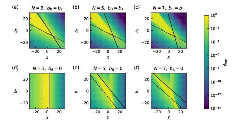
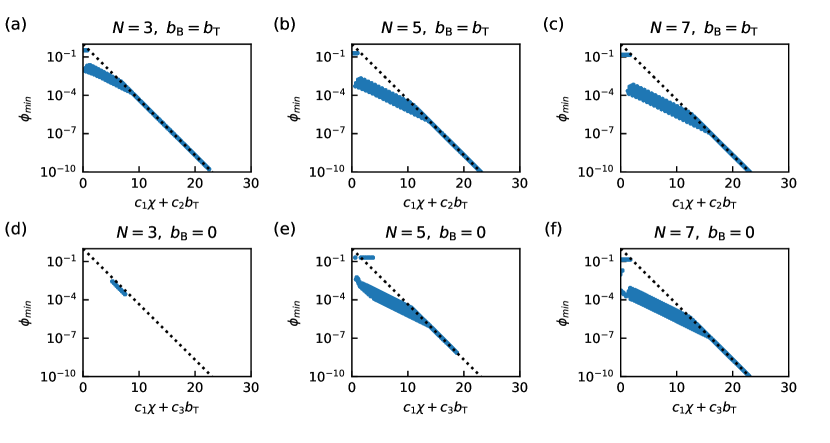
We first consider the special case where all species have the same volume fraction . We numerically solve Eqs.(4) and (5) in the main text and plot the number of species at different and in Fig. S1. The minimum volume fraction for all phases and species is plotted in Fig. S2.
When all volume fractions are identical we can analytically solve the eigenvalues of the Hessian matrix to find the instability criteria. For ,
| (17) |
For ,
| (18) |
The eigenvalues are
| (19a) | ||||
| (19b) | ||||
Solving equations we obtain
| (20a) | ||||
| (20b) | ||||
Using we have
| (21a) | ||||
| (21b) | ||||
In Fig. S1, Fig. S2, and Fig. 1(b) and Fig. 3(b) in the main text, the solid (dashed) black curve represents (). When they become
| (22a) | ||||
| (22b) | ||||
It is clear that can affect but does not appear in . From Fig. S1 we can see that the critical curves (black curves) predicted from linear stability analysis cannot capture the real transition when the three-body interactions are considered.
In this special case that all species have the same volume fraction , Eqs.(4) and (5) in the main text can be solved analytically for large interactions (, , and ). For large positive interactions, we know there are phases. The volume fractions in one phase can be written as where the high fraction and low fractions . In the other phases the volume fractions can be obtained by exchanging the -th with . The chemical potentials and are
| (23a) | ||||
| and | ||||
| (23b) | ||||
should satisfy and thus we have
| (24) |
Using , , and , we obtain
| (25) |
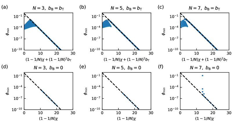
Hence,
| (26) |
This agrees with our numerical results shown in Fig. S3. Note that disappears in the expression of . If , is determined only by the pair interaction and the number of component . For , we find
| (27) |
We next focus on the strong attractive interaction regime. Here we have two phases with fractions and because of the symmetry of the interactions. Note that and . We have two equations
| (28) |
Specifically,
| (29) |
and
| (30) |
Sinces the lowest fraction is , we can assume , , and . Hence,
| (31a) | ||||
| and | ||||
| (31b) | ||||
The latter gives
| (32) |
Eq. 32 is consistent with numerical results for sufficient large interactions; see Fig. S4.
B.2 Ensemble average over different mean volume fractions
In Fig. S5 we plot the mean number of unstable modes obtained by sampling 100 different mean volume fractions that follows a uniform distribution [45]. In Fig. S6 we plot the mean number of unstable modes. In Fig. S7 we show the relative different of the mean phase number and the mean number of unstable modes plus one , defined as . All are qualitatively the same as the data shown in Fig. 5 in the main text.
We next explain how we obtain the boundary of the stable region, i.e., the black curves shown in Fig. 2, Fig. 4, and Fig. 5 in the main text. The only assumption is that the phase separation happens first when there are equivalent species. For a given , the stable region is the intersection of all the stable regions for all possible .
B.2.1 Stable region for
For and hence , the Hessian is
| (35) |
All eigenvalues should be larger than to ensure no phase separation can happen. We assume that because of symmetry and use ,
| (38) |
The eigenvalues are
| (39) |
or more specifically
| (40a) | ||||
| (40b) | ||||
Simultaneously satisfying for all possible leads to the black curves in Fig.2(a) in the main text.
Generally, for , the two eigenvalues are
| (41a) | ||||
| (41b) | ||||
The condition leads to
| (42) |
We define and need to find the minimum of . When , increases as increases, and hence , which is
| (43) |
which reduces to since . When , however,
| (44) |
which leads to
| (45) |
If , i.e., ,
| (46) |
and hence
| (47) |
If , then still . Taken together,
| (48) |
Hence, at gives the most strict criteria and hence it is still the boundary even if . For , it is more difficult because the minimum depends on both and . We know that if Eq. 41b with converges to
| (49) |
We numerically solve with Eq. 41b up to and find it agrees well with Eq. 49. This large limit boundary of the stable region is plotted as red dashed line in Fig. 5(vii) in the main text.
B.2.2 Stable region for
Now we consider . We obtain the two eigenvalues
| (50a) | ||||
| (50b) | ||||
Here, leads to
| (51) |
This is exactly the same as Eq. 42 if we replace by and hence we obtain
| (52) |
Similar to the case of , is more complicated but we can numerically obtain the boundary of the stable region, as the black curves shown in Fig. 5(iv–v) in the main text. We also plot the boundary for as the red dashed line in Fig. 5(v) in the main text.
B.2.3 Stable region for
Now we consider . We obtain the two eigenvalues
| (53a) | ||||
| (53b) | ||||
Here, leads to
| (54) |
Similar as before, we obtain the boundary of the stable region; see the black curves shown in Fig. 5(i–iii) in the main text. We also plot the boundary for as the red dashed line shown in Fig. 5(iii) in the main text.
Appendix C Extra results for random interactions
Here we report some results for Gaussian random interactions.
C.1 Stability analysis for identical volume fractions
We first consider the special case with identical volume fractions . The Hessian matrix in Eq. 9 becomes
| (55) |
We consider the system only with pair random interactions, i.e.,
| (56) |
This is well studied [41]. More specifically, there are eigenvalues that follows the semi-circle distribution
| (57) |
if where
| (58) |
and is the eigenvalue. One eigenvalue is asymptotically Gaussian distributed
| (59) |
We next add the higher-order interactions and assume that they also follow a normal distribution . We can construct an effective pair interaction
| (60) |
with the mean value
| (61) |
and the variance
| (62) |
Therefore, for identical volume fractions, the higher order interactions are trivial and can be represented by an effective pair interaction. Note that this good feature is based on the assumption that all elements follow the same distribution and are independent. In the model we considered in the main text, however, we need to be more careful because not all three-body interaction terms follow the the same normal distribution. For example, when , the elements are fixed to . Therefore, we need change the value in Eq. 62 by the real number of random elements and we denote it by . For , ; for , ; and for , . Therefore, we rescale the variance in Fig. 8 in the main text, by assuming that this also works for arbitrary mean volume fractions. A more strict way to analytically study this can follow [50].
C.2 Numerical results for different volume fractions
We have sampled different random interactions and different mean volume fractions for each point . Fig. S8 and Fig. S9 are the figure for and respectively, similar to Fig. 7 in the main text. Fig. S10, Fig. S11 and Fig. S12 show the differences for , respectively. All results demonstrate that . Fig. S13 shows the phase count scaled by the number of components.