Experimental realization of universal quantum gates and six-qubit state
using photonic quantum walk

Abstract

Controlled quantum walk forms the basis for various quantum algorithm and quantum simulation schemes. Though theoretical proposals are also available to realize universal quantum computation using quantum walks, no experimental demonstration of universal set of gates has been reported. Here we report the experimental realize of universal set of quantum gates using photonic quantum walk. Taking cue from the discrete-time quantum walk formalism, we encode multiple qubits using polarization and paths degree of freedom for photon and demonstrate realization of universal set of gates with 100% success probability and high fidelity, as characterised by quantum state tomography. For a 3-qubit system we encode first qubit with $H$ and $V-$polarization of photon and path information for the second and third qubit, closely resembling a Mach-Zehnder interference setup. To generate a 6-qubit system and demonstrate 6-qubit GHZ state, entangled photon pairs are used as source to two 3-qubit systems. We also provide insights into the mapping of quantum circuits to quantum walk operations on photons and way to resourcefully scale. This work marks a significant progress towards using photonic quantum walk for quantum computing. It also provides a framework for photonic quantum computing using lesser number of photons in combination with path degree of freedom to increase the success rate of multi-qubit gate operations.

I Introduction

Quantum computers hold the potential to solve problems that are too complex for classical computers. They are also poised to efficiently mimic-understand various complex, inaccessible quantum systems in nature by harnessing and controlling quantum mechanical principles namely, superposition, interference and entanglement. While we’re yet to construct a practical quantum computer of a sufficient size, numerous quantum algorithms have been developed and demonstrated in various quantum computing platform that is being developed [1, 2, 3, 4, 5, 6, 7, 8, 9]. Multiple schemes for realizing qubits and to perform quantum operations have been developed for each quantum computing platform. Among them, photonic platform are being developed using multiple approaches where discrete-variable, continuous-variable, measurement based and fusion based approach are prominent to note [10, 11, 12]. Though photons are robust against noise compared to other systems, they have their own disadvantages. For example, in discrete-variable approach the multi-qubit gate operations are probabilistic in nature due to natural restriction in photon-photon interaction, reducing the success probability of a computational task [13, 14, 15]. Any improvement to increase multi-qubit gate operations will help in boosting the potential of discrete-variable approach for photonic quantum computation.

Quantum walks, which have both continuous-time and discrete-time variants, have played a fundamental role in development of quantum algorithms [16, 17, 18] and schemes for quantum simulations [19, 20, 21, 22, 23, 24, 25, 26, 27, 28, 29]. One-dimensional discrete-time quantum walks have been employed to engineer various high-dimensional quantum states, showcasing their versatility [30, 31]. These walks can be experimentally implemented, such as in linear optical systems controlling polarization-path and other degree of freedom of single photon states [32, 37, 34, 36, 33, 35, 38]. They also provide the basis for implementing quantum gates [39, 40, 41, 42, 43]. This implies that the universal quantum computation can be realized using quantum walk operations. While quantum computing model has been developed using both, continuous-time and discrete-time quantum walk, our model, based on discrete-time quantum walk [42, 43], offers a more tangible and logical foundation for photonic quantum computing architecture. It maps position-based states to qubit states and in addition to that polarization state is also a qubit state. This helps in implementing polarization controlled operations, thus conducts quantum computations by emulating gates through unitary evolution. This approach provides a physical and structured framework for photonic quantum computation, which is instrumental for building quantum processors.

One of the main criteria for a system to be considered for universal quantum computation is its ability to implement a universal set of quantum gates. The universal gate set typically includes single-qubit gates like phase (P) and Hadamard (H) gates, along with the two-qubit controlled-NOT (CNOT) gate. The focus of this work is to harness the power of single-particle photonic discrete-time quantum walk to experimentally demonstrate a three-qubit universal quantum computation and configure a six-qubit system using entangled photon pairs in combination of three-qubit systems. For experimental demonstration of gates operation on 3-qubit system we use heralded single photons from spontaneous parametric down conversion (SPDC) process and control its propagation on four path degree of freedom. To demonstrate a 6-qubit system two 3-qubit system units are combined using an entangled photon source. At a three qubit level involving only single photon and its interference along paths, all multi-qubit gate operations are definite and not probabilistic in nature making it a robust scheme. We report high fidelity of all universal quantum gate operations as characterised by quantum state tomography involving about 28 gate operations including quantum state preparation on a 3-qubit system. At 6-qubit level controlling the entanglement between the two-photons, each 3-qubit systems can be engineered to demonstrate control on the composite 6-qubit system and we use 6-qubit system and generate GHZ state. This work provides a scalable framework for photonic quantum computing using lesser number of photons in combination with path degree of freedom to increase the success rate of multi-qubit gate operations.

II PHOTONIC QUANTUM WALK AND UNIVERSAL QUANTUM GATES

The dynamics of a one-dimensional discrete-time quantum walk is defined on a configuration of Hilbert space composing of an internal degree of freedom of a particle and position space, $\mathcal{H}_{w}=\mathcal{H}_{C}\otimes\mathcal{H}_{S}$ [44, 45]. For a photonic quantum walk, coin space can be configured to be spanned by the horizontal and vertical polarization states of the photon $\mathcal{H}_{C}=span${$\ket{H},\ket{V}$} and the description of the position space corresponds to the various paths a photon can take, and its dimensionality depends on the specific requirements of the problem. Typically, on an one-dimensional position space it is denoted as $\mathcal{H}_{S}=span${$\ket{-x},,.......,\ket{-1},\ket{0},\ket{1},...,\ket{x}$} representing a range of possible positions or paths that the photon can occupy.

The standard evolution of each step in this quantum walk is defined using two sequential operations. First, is the unitary quantum coin operation, a non-orthogonal unitary operator that solely acts on the coin space and it is followed by the conditional position shift operation. A general coin operation would be a $U(2)$ matrix consisting of 4 parameters,

$$C(\tau,\eta,\zeta,\theta)=e^{i\tau}\begin{bmatrix}e^{i\eta}\cos(\theta)&e^{i\zeta}\sin(\theta)\\ -e^{-i\zeta}\sin(\theta)&e^{-i\eta}\cos(\theta)\\ \end{bmatrix}$$ (1)

and shift-operation takes the form,

$$S=\sum_{x}(|H\rangle\langle H|\otimes|x-1\rangle\langle x|+|V\rangle\langle V|\otimes|x+1\rangle\langle x|).$$

After $t$-step of evolution the polarization-path state of the photon would be,

$$|\Psi\rangle_{P-P}=[S(C(\theta))\otimes\mathbb{I}]^{t}(\alpha|H\rangle+\beta|V\rangle)\otimes|x\rangle.$$ (2)

We can experimentally achieve full polarization control of a single photon using a combination of Quarter-Half-Quarter waveplates (Q-H-Q), if we neglect the global phase of $C(\tau,\eta,\zeta,\theta)$, i.e. $\tau$ [46]. The encoding of its path is accomplished by applying a beamsplitter (BS) or a polarizing beam splitter (PBS) at each step. The choice between using a PBS or a BS depends on the specific operational requirements. In different setting various realization of photonic quantum walk has already been experimentally demonstrated.

The universal set of quantum gates for quantum computation consists of two single-qubit gates: the Phase gate ($P$) and the Hadamard gate ($H$), along with one two-qubit gate, the controlled-NOT gate ($CNOT$). In mathematical form, it can be represented as follows,

$$U=\left(\begin{bmatrix}1&0\\ 0&e^{i\pi/4}\end{bmatrix},\frac{1}{\sqrt{2}}\begin{bmatrix}1&1\\ 1&-1\end{bmatrix},\begin{bmatrix}1&0&0&0\\ 0&1&0&0\\ 0&0&0&1\\ 0&0&1&0\end{bmatrix}\right).$$

These three gates, along with the single-qubit Pauli gates form a universal gate set. This means that we can achieve optimal accuracy for any operation according to our needs simply by applying these gates.

For the quantum computation model using discrete-time quantum walk a general form of shift operators and quantum coin operator is defined in Ref. [43, 42]. The shift operations are configured to enable control on the shift of the particle to either left or to the right along with retaining in the same path (position) conditioned on the coin-state of the particle. In consolidated form it looks like,

$$S_{\pm}^{k}=\sum_{l\in\mathbb{Z}}\Bigr{[}\ket{k}\bra{k}\otimes\ket{l\pm 1\;\textrm{mod}\;m}\bra{l}+\sum_{i\neq j}^{\mu}\ket{i}\bra{i}\otimes\ket{l}\bra{l}\Bigr{]},$$ (3)

where $\mu$ is internal degree of freedom and $S^{0}_{+}$ or $S^{0}_{-}$ dictates the particle to the right or left if the coin-state is $\ket{0}$ representing the polarization state of photon $\ket{H}$, respectively. Similarly, $S^{1}_{+}$ and $S^{1}_{-}$ will act for $\ket{1}$ representing the polorization state of photon $\ket{V}$, this type of shift operation can be achieved using a combination of half-waveplates (HWP) and PBS. The $mod\;m$ comes for a closed graph dynamics of the quantum walk. The collection of operators $\{S^{0}_{\pm},S_{\pm}^{1},C(\tau,\eta,\zeta,\theta),\mathbb{I}\}$ constitutes a versatile set of operators representing the quantum walk. Moreover, this set of operators can be effectively employed to realize the universal set of quantum-gates within the discrete-time quantum walk framework.

III Encoding qubits and Universal gate implementation

Encoding the qubit in the basis of polarization degree of freedom of photon and path degree of freedom for the photon forms the basis for photonic quantum computing presented here. For example, using polarization state of a photon and four path basis, one can define a 3-qubit system where one qubit will be the polarization degree of freedom of photon and other two qubits will be defined on the position basis. Although it is possible to extend the number of available paths for photons and increase the realisable number of qubits, it does not scale resourcefully. Here we will present the encoding to qubits in polarization and path basis first and address the scalability after that.

Polarization information as qubit : A general polarization state of a photon can be spanned by the two basis states, $\{\ket{H},\ket{V}\}$, where $H$ and $V$ represents, horizontal and vertical polarization, respectively. Finally the general qubit $|\psi\rangle$ can be written as

$$\ket{\psi}=\cos\left(\frac{\theta}{2}\right)\ket{H}+e^{i\phi}\sin\left(\frac{\theta}{2}\right)\ket{V}.$$ (4)

Here $\theta\in[0,\pi]$ and $\phi\in[0,2\pi)$ varying these parameters we can generate all the possible polarization states i.e. it helps us to map any point on the Bloch-Sphere. Experimentally, we can achieve all polarization pure states using a combination of Quarter-Half-Quarter (Q-H-Q) waveplates introduced in the path of a single photon source. Moreover, we can use any combination of these three waveplates, i.e., Q-Q-H or H-Q-Q, to prepare any arbitrary superposition.

HWP and Quarter-Wave Plates (QWP) are characterized by matrix structures derived from Jones Calculus, represented as follows:

$$\begin{gathered}H(x)=\begin{pmatrix}\cos 2x&\sin 2x\\ \sin 2x&-\cos 2x\end{pmatrix}\\ \\ Q(x)=e^{-i\pi/4}\begin{pmatrix}{\cos^{2}x}+i\sin^{2}x&(1-i)\sin{x}\cos{x}\\ (1-i)\sin{x}\cos{x}&i\cos^{2}x+\sin^{2}x\end{pmatrix}.\end{gathered}$$ (5)

Pauli matrices {$\sigma_{x}$, $\sigma_{y}$, $\sigma_{z}$} don’t belong to $SU(2)$ because their determinant is -1. In contrast, HWP and QWP have determinant values of -1 and +1, respectively, based on their matrix structures. Then the determinant of Q-H-Q will be -1.

The set of Pauli matrices along with identity($\mathds{I}_{2})$, $\{\mathds{I}_{2},\sigma_{x},\sigma_{y},\sigma_{z}\}$, form a basis for unitary matrices in the $(2\times 2)$ space. By choosing the proper angles of Q-H-Q we can get all the Pauli matrices, enabling all the single-qubit operations on polarization qubits. It is written as follows,

• X: $(0,\frac{\pi}{4},0)$, $\sigma_{x}$:= $\begin{bmatrix}0&1\\ 1&0\end{bmatrix}$

• Y: $(\frac{\pi}{2},-\frac{\pi}{4},0)$, $\sigma_{y}$:= $\begin{bmatrix}0&-i\\ i&0\end{bmatrix}$

• Z: $(0,{\pi},\frac{\pi}{2})$, $\sigma_{z}$:= $\begin{bmatrix}1&0\\ 0&-1\end{bmatrix}$

• S($\pi/2$): $(\frac{\pi}{4},\frac{7\pi}{8},\frac{5\pi}{4})$ := $e^{i\pi/4}\begin{bmatrix}1&0\\ 0&e^{i\pi/2}\end{bmatrix}$

• P($\pi/4$): $(\frac{3\pi}{4},\frac{3\pi}{16},\frac{3\pi}{4})$ := $-e^{-i\pi/8}\begin{bmatrix}1&0\\ 0&e^{i\pi/4}\end{bmatrix}$

This describes how we can achieve all sorts of single-qubit operations via Q-H-Q on polarization qubit.

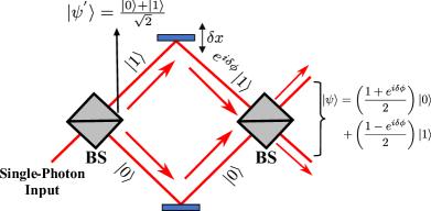
Figure 1: The schematic depicts how we can utilize the Mach-Zehnder Interferometer to form a basis for path qubit states. Apart from that it illustrates the Hadamard operation on the path qubit twice for the balanced case scenario. In other words, the operation at the first BS can be conceptualized as a unitary operation $U=\mathbb{I}_{2}\otimes\textrm{H}$, and similarly, the operation at the second BS is the same. High visibility of interference, ensures the good fidelity of the two simultaneous Hadamard operations on the path.

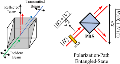
Figure 2: The left figure illustrates the operation of a PBS, while the right figure demonstrates the generation of the Bell state $\ket{\phi^{+}}=\frac{\ket{00}+\ket{11}}{\sqrt{2}}$ in polarization and path degree of freedom. When an HWP is set at $22.5^{\circ}$, it transforms the photon state from $\ket{H}$ to $\frac{\ket{H}+\ket{V}}{\sqrt{2}}$. After passing through a PBS, the resulting state becomes $\ket{\psi}_{P-P}=\frac{\ket{H}\ket{0}+\ket{V}\ket{1}}{\sqrt{2}}$.

Path information as qubit : Path encoding becomes most comprehensible through the lens of a Mach-Zender interferometer designed for a single photon. This setup involves the photon initially encountering a beam splitter, at which point it can choose between two feasible paths, denoted as $\ket{0}$ (the lower path) and $\ket{1}$ (the upper path). By introducing a phase delay in the $\ket{1}$ path using a slide, the system takes on the configuration depicted in the Fig. 1. Upon recombination of the two path components at another beam splitter, the final state materializes as $|\psi\rangle=\frac{(1+e^{i\delta\phi})}{2}\ket{0}+\frac{(1-e^{i\delta\phi})}{2}\ket{1}$. This culminates in the emergence of an interference pattern that transforms as $\phi$ varies.

Remarkably, from the standpoint of information encoding, manipulating $\delta\phi$ permits the attainment of all fundamental states $\ket{+},\ket{-},\ket{L},\ket{R}$. This intriguing feature underscores the versatility of path encoding and its potential for information manipulation within the quantum domain. In our context, path encoding initially disregards polarization information. However, for a comprehensive description of polarization-path encoding, we must consider the polarization of each path, resulting in a Hilbert space denoted as $\mathcal{H}_{P-P}=\mathcal{H}_{Pol.}\otimes\mathcal{H}_{Path}$, encompassing a total of four modes of a single photon (2-polarization, 2-path), effectively representing the polarization-path quantum state. The general 2-qubit state can be expressed as:

$$\ket{\Psi}_{\textrm{Gen}}=\alpha\ket{H}\ket{0}+\beta\ket{H}\ket{1}+\gamma\ket{V}\ket{0}+\delta\ket{V}\ket{1}$$ (6)

where $\{\alpha,\beta,\gamma,\delta\}\in\mathcal{C}$ and $|\alpha|^{2}+|\beta|^{2}+|\gamma|^{2}+|\delta|^{2}=1$.

Method of preparation of these type of state is detailed in the supplementary material. The computational basis takes the form - $\ket{H}\ket{0}=\ket{00}$, $\ket{H}\ket{1}=\ket{01}$, $\ket{V}\ket{0}=\ket{10}$ and $\ket{V}\ket{1}=\ket{11}$. To prepare 2-qubit maximally entangled states (i.e., Bell states) in polarization-path encoding, we can use a PBS instead of a BS. A concise description of PBS is illustrated in Fig. 2, the input state of light in polarization and path is - $\ket{\psi}_{in}=(\alpha\ket{H}+\beta\ket{V})\ket{0}$, where the $\ket{0}$ represent the path in which the photon is, then the output state would be $\ket{\psi}_{out}=\alpha\ket{H}\ket{0}+\beta\ket{V}\ket{1}$, so now it becomes a polarization-path entangled state.

1- and 2-qubit gate implementation : The 2-qubit system we will present here is a composition of polarization degree of freedom of photon as qubit 1 and path degree of freedom for photons to travel as qubit 2. Optical scheme for 2-qubit state preparation and implementation of universal gates are illustrated in Fig. 3. Implementation of gates is a composition of a path-dependent quantum coin operation realized using Q-H-Q or other combination of waveplates and conditioned shift operator using PBS or BS. We can note that for realizing Hadamard operation on path encoded qubit needs a single photon interference setup whereas realizing CNOT gates are relatively easier.

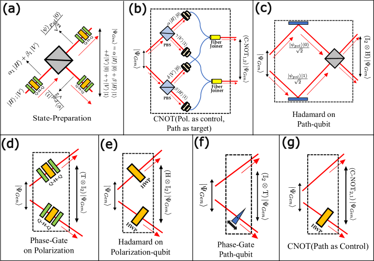
Figure 3: Illustration of all the two-qubit gate operations necessary for achieving universal quantum computing using the discrete-time single-particle quantum walk approach. (a) It demonstrates how a general 2-qubit state can be generated using beam-splitters and Q-H-Qs.(b)-(g) depict the specific gates realization with appropriate label.

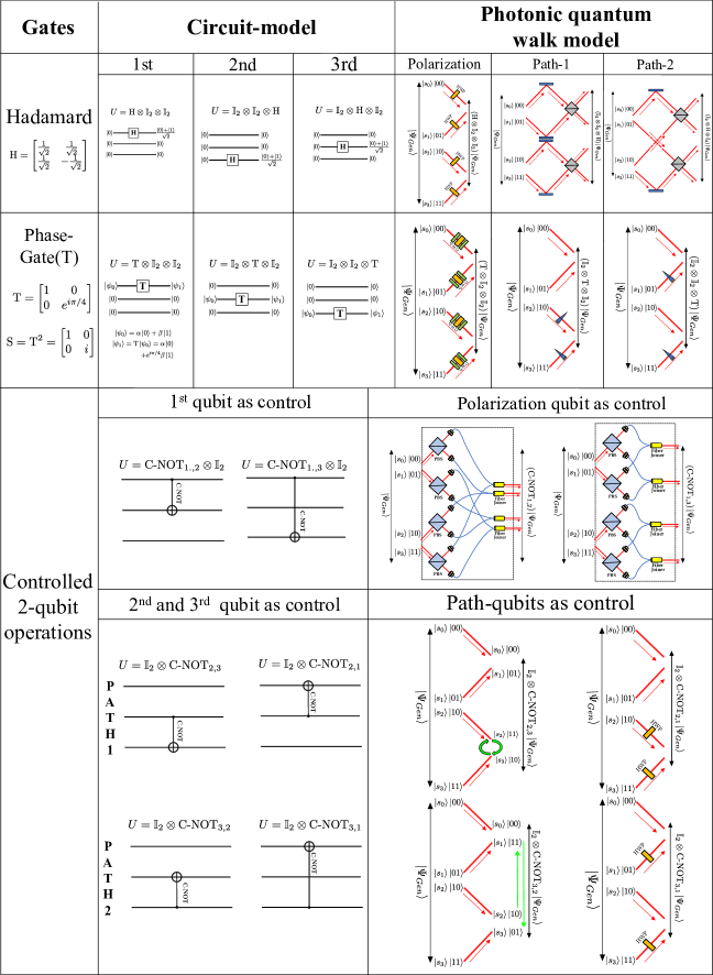
Figure 4: Table provides a comprehensive description of a full 3-qubit representation of single-particle photonic quantum walk, alongside a comparison with the circuit model representation. In our scenario, the polarization of the single photon serves as the first qubit, while the four-path degree of freedom serves as the other two qubits.

For a 2-qubit realization, heralded single-photons of 810nm obtained from spontaneous parametric down conversion (SPDC) using PPKTP crystal was used. The quantum state tomography scheme used to reconstruct the density matrix is detailed in the supplementary material, involving additional path interference and polarization manipulation using Q-H-Q. For experimental purposes, we have also demonstrated the visibility pattern of the interferometer. To experimentally obtain the gate fidalities, initial state was first prepared to $|\Psi\rangle_{in}=\frac{1}{\sqrt{2}}[|00\rangle+|11\rangle]$ and the gate operations were implemented. Starting from state preparation to quantum state tomography, around 10 gate operations were executed. The experimentally obtained gate fidalities from quantum state tomography are given in Table 1.

Table 1: Fidelity of 2-qubit gate operation

Gate	$\textrm{H}\otimes\mathbb{I}_{2}$	$\textrm{T}\otimes\mathbb{I}_{2}$	$\textrm{C-NOT}_{1,2}$	$\mathbb{I}_{2}\otimes\textrm{H}$	$\mathbb{I}_{2}\otimes\textrm{T}$	$\textrm{C-NOT}_{2,1}$
Fidelity	0.97	0.92	0.89	0.95	0.91	0.96

IV 3- and 6-qubit system

For 3-qubit system, polarization degree of freedom of photon represents qubit 1 and four path degree of freedom for photons represent qubit 2 and qubit 3. The universal gate operation on 3-qubit system in a standard circuit model and its equivalent optical scheme in the polarization-path encloded 3-qubit system is illustrated in Fig. 4. One can note that realizing Hadamard operation on path encoded qubit involves interfereometry and realizing CNOT gate which is usually difficult in other setup are easily realizable by swapping the paths in this scheme.

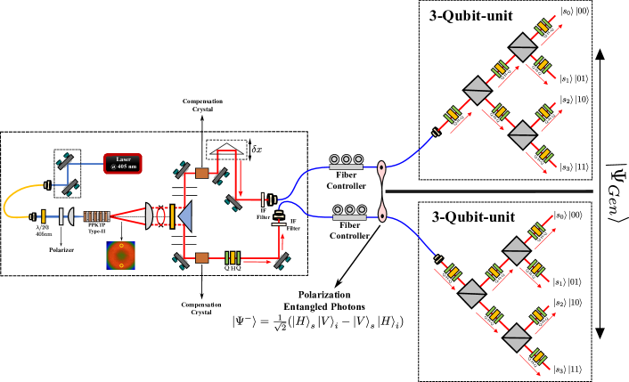
Figure 5: The first part of the experimental setup involves generation of entangled photons from SPDC process using type II PPKTP crystal. Subsequently, the two photons are fiber-coupled using a fiber controller before being directed to two separate 3-qubit units, shown to the right. Utilizing the entanglement, we can connect the distinct 3-qubit units and perform the necessary gates as required on each 3-qubit unit..

Table 2: Fidelity of 3-qubit gate operation

Gate	$\mathbb{I}_{2}\otimes\textrm{C-NOT}_{3,2}$	$\mathbb{I}_{2}\otimes\textrm{C-NOT}_{3,1}$	$\mathbb{I}_{2}\otimes\textrm{C-NOT}_{2,3}$	$\mathbb{I}_{2}\otimes\textrm{C-NOT}_{2,1}$	$\textrm{C-NOT}_{1,2}\otimes\mathbb{I}_{2}$	$\textrm{C-NOT}_{1,3}\otimes\mathbb{I}_{2}$
Fidelity	0.98	0.93	0.99	0.94	0.86	0.88

To calculate the fidelities of the gate operations, starting from the 3-qubit general state preparation to performing quantum state tomography, maximum of 28 gate operations were executed. The experimentally obtained gate fidelities are given in Table 2. Since the fidelities of Hadamard operations are same as given in Table 1, only CNOT operations for different combination of qubits are given. We can note that the fidelity of CNOT gate between two path qubits is very high when compared to CNOT between the polarization and path qubits. This is because to use of only swapping of path between path qubits to implement CNOT gate. This allows for efficient handling multi-qubit operations using path basis.

One of the method to realize 6-qubit system is illustrated in Fig. 5. A 6-qubit system is sourced by the, entangled photon pair given by $\ket{\Psi}=1/\sqrt{2}(\ket{H}\ket{V}-\ket{V}\ket{H})$ generated from the SPDC process. Each photon from the entangled pair are used as an input to two separate 3-qubit systems. Various operations on the 6-qubit system can be configured first by controlling entanglement between the two photons and these two photons are sourced to the two 3-qubit systems where gate operations are performed as discussed for 3-qubit system earlier. For example, we can easily convert entangled state to the state $\ket{\Psi^{{}^{\prime}}}=1/\sqrt{2}(\ket{H}\ket{H}-\ket{V}\ket{V})$ using HWP in one of the the arm (signal arm). By placing a PBS in the two separate 3 qubit units we can generate the 6-qubit GHZ state

$$\ket{\Psi}_{GHZ}=\frac{1}{\sqrt{2}}(\ket{0}^{\otimes 6}-\ket{1}^{\otimes 6}).$$

Though all the 6 qubits in the system are not completely connected to one another, through entangled photon pairs they can be connected and engineered to control a 6-qubit system.

Scaling : Number of qubits can be scaled by using multiple four path basis in a tensor network configuration of 2-qubits and entangling them with a single photon as as given in the mathematical model of the scheme [42, 43]. However, single photon in multiple network of two-qubit position basis will results in loss of fidelity. As demonstrated for 6-qubit here, further scaling with a combination of six-qubit systems can be explored by further entangled in other degree’s of freedom of photons. However, involving more photons will make the connection between the each units of smaller qubits probabilistic but overall efficiency will be better than the standard approach of using single photon in dual rail encoding to represent each qubits.

V Conclusion

In this work we have reported the experimental demonstration of realizing universal set of quantum gates using photonic quantum walk. In the scheme, multiple qubits were encoded using polarization and paths degree of freedom for and universal quantum gates were implemented with 100% success probability, and high fidelity. The fidelity was characterised by quantum state tomography. For a 2-qubit and 3-qubit system, the first qubit was encoded with polarization state of photon and path information was used for encoding other qubits. For the 6-qubit system an entangled photon pairs from SPDC process was used to source two 3-qubit units and realize full 6-qubit GHZ state. In the scheme only one photon is involved to realize 2-qubit and 3-qubit system. Not invoking photon-photon interaction has resulted in very high fidelity of gate operations. This also makes all the gates operation a definite realizaiton. Fidelities directly accounts for experimental inaccuraries involved in the process. We have demonstrated that some of the two-qubit gates, CNOT between path qubits, are easily realizable in the scheme compared to other approaches. The high fidealities obtained after implementing 10 and 28 gates operation on 2-qubit and 3-qubit systems inlcuding state preparation and quantum state tomography are very promising. This indicates a promising progress towards using photonic quantum walk for quantum computing and provide a general framework for photonic quantum computing using lesser number of photons in combination with path and other degree of freedom of photons.

Acknowledgement
We would like to thank Dr. Prateek Chawla for useful discussions on some of the schemes for optical realization. We acknowledge the support from the Office of Principal Scientific Advisor to the Government of India, project no. Prn.SA/QSim/2020.

Supplemental Materials: Experimental realization of universal quantum gates and six-qubit state using photonic quantum walk

V.1 Quantum State Tomography $\And$ Measurement

In this section we will describe the measurement part, how quantum state tomography is done via various projective measurements on a different basis. It will help us to reconstruct the density matrix. So, we need to define the different bases and know that we need $2^{2N}$ projective measurement to get the entire density matrix, where N is the number of qubits.

The number of qubits is 2, so we need 16 measurements. At first, the new basis states are

$$\ket{0^{\prime}},\ket{1^{\prime}}=\frac{\ket{0}\pm\ket{1}}{\sqrt{2}}\equiv\ket{D},\ket{A}\qquad\ket{0^{\prime\prime}},\ket{1^{\prime\prime}}=\frac{\ket{0}\pm i\ket{1}}{\sqrt{2}}\equiv\ket{L},\ket{R}$$ (7)

Here, $\ket{D}$, $\ket{A}$ represents diagonal and anti-diagonal states and $\ket{L}$, $|\ket{R}$ represents left circular and right circular polarization of light. Similarly, we have to define 3 sets of basis states in qubit involving path information of the photon, here $\ket{0}$ and $\ket{1}$ represent to path in the state preparation.

Now, the Pauli-matrices are Hermitian, and together with the identity matrix $\mathds{1}$ (sometimes considered as the zeroth Pauli matrix $\sigma_{0}$), the Pauli matrices form a basis for the vector space of $2\times 2$ Hermitian matrices. This means that any $2\times 2$ Hermitian matrix can be written uniquely as a linear combination of Pauli matrices.

It implies any Hermitian can be represented by a linear combination of these 4 matrices then we also represent the 1 qubit density matrix using these operators. Also, we know that

$$\begin{split}\hat{\sigma}_{0}=\begin{bmatrix}1&0\\ 0&1\end{bmatrix}=|H\rangle\langle H|+|V\rangle\langle V|\;;\;\hat{\sigma}_{1}=\begin{bmatrix}0&1\\ 1&0\end{bmatrix}=|D\rangle\langle D|-|A\rangle\langle A|\\ \hat{\sigma}_{2}=\begin{bmatrix}0&-i\\ i&0\end{bmatrix}=|R\rangle\langle R|-|L\rangle\langle L|\;;\;\hat{\sigma}_{3}=\begin{bmatrix}1&0\\ 0&-1\end{bmatrix}=|H\rangle\langle H|-|V\rangle\langle V|\end{split}$$ (8)

Finally, we can write the density matrix as -

$$\hat{\rho}=\frac{1}{2}\sum_{i=0}^{3}S_{i}\hat{\sigma_{i}}\;\;\;;\;\;\;S_{i}\equiv\textrm{Tr}\{\hat{\sigma}_{i}\rho\}$$ (9)

$S_{i}$ are know are as the Stokes parameters. For pure states, we have $\sum_{i=0}^{3}S_{i}^{2}=1$ ; for mixed states, $\sum_{i=0}^{2}S_{i}^{2}<1$ and for the completely mixed state, $\sum_{i=0}^{3}S_{i}^{2}=0$. Upon imposing normalization, $S_{0}$ will always be 1. These values are essentially the results of various orthogonal projective measurements:

$$S_{0} =P_{|H\rangle}+P_{|V\rangle}\;;\;S_{1}=P_{|D\rangle}-P_{|A\rangle}$$ (10)

$$S_{2} =P_{|R\rangle}-P_{|L\rangle}\;;\;S_{3}=P_{|H\rangle}-P_{|V\rangle}$$

Similarly, we can map this situation to an N-qubit case, i.e. an N-qubit density matrix can be written as -

$$\hat{\rho_{N}}=\frac{1}{2^{N}}\sum_{i_{1},i_{2},...i_{N}=0}^{3}S_{i_{1},i_{2},...i_{N}}\hat{\sigma}_{i_{1}}\otimes\hat{\sigma}_{i_{2}}...\otimes\hat{\sigma}_{i_{N}}$$ (11)

Normalization condition leaves $S_{0,0,...,0}=1$; that leaves us to calculate $2^{2N}-1$ projective measurement to be done to reconstruct the density matrix.

$$S_{i_{1},i_{2},...,i_{N}}=\mathrm{Tr}\left(\{\hat{\sigma}_{i_{1}}\otimes\hat{\sigma}_{i_{2}}\otimes\dots\otimes\hat{\sigma}_{i_{N}}\}\cdot\hat{\rho}_{N}\right)$$ (12)

More easily, we can write these ”General Stokes Parameter” as -

$$S_{i_{1},i_{2},...,i_{N}}=(P_{\ket{\psi_{i_{1}}}}\pm P_{\ket{\psi_{i_{1}}^{\perp}}})\otimes(P_{\ket{\psi_{i_{2}}}}\pm P_{\ket{\psi_{i_{2}}^{\perp}}})\otimes...\otimes(P_{\ket{\psi_{i_{N}}}}\pm P_{\ket{\psi_{i_{N}}^{\perp}}})$$ (13)

all $i_{1},i_{2}...i_{N}$ runs from $\{0,1,2,3\}$, the $\{+\}$ sign appears for 0, and $\{-\}$ appears for 1,2,3

Clearly, for a 2-qubit case, we need 15 measurements. A general 2 qubit density matrix would be -

$$\hat{\rho_{2}}=\frac{1}{4}\sum_{i_{1},i_{2}=0}^{3}S_{{i_{1}},{i_{2}}}\hat{\sigma}_{i_{1}}\otimes\hat{\sigma}_{i_{2}}$$ (14)

For a 2-qubit setup, we will require 4 detectors to make simultaneous measurements. Choosing the measurement basis for each qubit leads to a particular setting and the detection pattern can be mapped to a particular measurement outcome. Each setting can give 4 possible measurement outcomes, leading to determining 4 of those probability values. We need 36 such probability values: $P_{|\psi_{1}\rangle|\psi_{2}\rangle}$where $|\psi_{1}\rangle,|\psi_{2}\rangle\in\{|H\rangle,|V\rangle,|D\rangle,|A\rangle,|R\rangle,|L\rangle\}$. Thus, 9 measurement settings are required instead of 15.

The Stokes parameters for a 2-qubit system polarisation state are -

$$S_{00}=1,\qquad S_{20}=P_{LH}+P_{LV}-P_{RH}-P_{RV},$$

$$S_{01}=P_{HD}-P_{HA}+P_{VD}-P_{VA},\qquad S_{21}=P_{RD}-P_{RA}-P_{LD}+P_{LA},$$

$$S_{02}=P_{HL}-P_{HR}+P_{VL}-P_{VR},\qquad S_{22}=P_{LD}-P_{LA}-P_{RD}+P_{RA},$$

$$S_{03}=P_{HH}-P_{HV}+P_{VH}-P_{VV},\qquad S_{23}=P_{LH}-P_{LV}-P_{RH}+P_{RV},$$

$$S_{10}=P_{DH}+P_{DV}-P_{AH}-P_{AV},\qquad S_{30}=P_{HH}+P_{HV}-P_{VH}-P_{VV},$$

$$S_{11}=P_{DD}-P_{DA}-P_{AD}+P_{AA},\qquad S_{31}=P_{HD}-P_{HA}-P_{VD}+P_{VA},$$

$$S_{12}=P_{DL}-P_{DR}-P_{AL}+P_{AR},\qquad S_{32}=P_{HL}-P_{HR}-P_{VL}+P_{VR},$$

$$S_{13}=P_{DH}-P_{DV}-P_{AH}+P_{AV},\qquad S_{33}=P_{HH}-P_{HV}-P_{VH}+P_{VV}.$$

Since, in our setup, 1st qubit is represented by the polarization of the photon, and the path information represents the 2nd qubit, for that purpose we have to change our notation, for example - $P_{HH}$ would be $P_{00}$ it implies $0$ and $1$ belongs to computational basis, $\ket{0^{\prime}}=\frac{\ket{0}+\ket{1}}{\sqrt{2}}$ and $\ket{1^{\prime}}=\frac{\ket{0}-\ket{1}}{\sqrt{2}}$, finally $\ket{0^{\prime\prime}}=\frac{\ket{0}+i\ket{1}}{\sqrt{2}}$ and $\ket{1^{\prime\prime}}=\frac{\ket{0}-i\ket{1}}{\sqrt{2}}$ the entire list is -

$P_{HH}=P_{00}$ , $P_{HV}=P_{01}$ , $P_{HD}=P_{00^{\prime}}$ , $P_{HA}=P_{01^{\prime}}$ , $P_{HL}=P_{00^{\prime\prime}}$ , $P_{HR}=P_{01^{\prime\prime}}$

$P_{VH}=P_{10}$ , $P_{VV}=P_{11}$ , $P_{VD}=P_{10^{\prime}}$ , $P_{VA}=P_{11^{\prime}}$ , $P_{VL}=P_{10^{\prime\prime}}$ , $P_{VR}=P_{11^{\prime\prime}}$

$P_{DH}=P_{0^{\prime}0}$ , $P_{DV}=P_{0^{\prime}1}$ , $P_{DD}=P_{0^{\prime}0^{\prime}}$ , $P_{DA}=P_{0^{\prime}1^{\prime}}$ , $P_{DL}=P_{0^{\prime}0^{\prime\prime}}$ , $P_{DR}=P_{0^{\prime}1^{\prime\prime}}$

$P_{AH}=P_{1^{\prime}0}$ , $P_{AV}=P_{1^{\prime}1}$ , $P_{AD}=P_{1^{\prime}0^{\prime}}$ , $P_{AA}=P_{1^{\prime}1^{\prime}}$ , $P_{AL}=P_{1^{\prime}0^{\prime\prime}}$ , $P_{AR}=P_{1^{\prime}1^{\prime\prime}}$

$P_{LH}=P_{0^{\prime\prime}0}$ , $P_{LV}=P_{0^{\prime\prime}1}$ , $P_{LD}=P_{0^{\prime\prime}0^{\prime}}$ , $P_{LA}=P_{0^{\prime\prime}1^{\prime}}$ , $P_{LL}=P_{0^{\prime\prime}0^{\prime\prime}}$ , $P_{LR}=P_{0^{\prime\prime}1^{\prime\prime}}$

$P_{RH}=P_{1^{\prime\prime}0}$ , $P_{RV}=P_{1^{\prime\prime}1}$ , $P_{RD}=P_{1^{\prime\prime}0^{\prime}}$ , $P_{RA}=P_{1^{\prime\prime}1^{\prime}}$ , $P_{RL}=P_{1^{\prime\prime}0^{\prime\prime}}$ , $P_{RR}=P_{1^{\prime\prime}1^{\prime\prime}}$

We will now represent the state in different bases, examine the coefficients that emerge, and subsequently apply our setup and interference effects to calculate the projective measurements as probabilities. We will do this by changing the polarization state and interference effects.

Rather than delving into the orthogonal basis of each qubit during tomography, we will adjust the polarization amplitudes of both the individual paths and their interference to attain the necessary coefficients. This section elucidates how these various measurements are conducted -

The state is already written in the basis

$$\{(\ket{0},\ket{1});(\ket{0},\ket{1})\}\Rightarrow\ket{\psi}=\alpha\ket{0}\ket{0}+\beta\ket{0}\ket{1}+\gamma\ket{1}\ket{0}+\delta\ket{1}\ket{1}$$

it provides the projection values $\{P_{00},P_{01},P_{10},P_{11}\}$ And for all the other basis the state and the projection operators are enlisted -

1. $$\{(\ket{0},\ket{1});(\ket{0^{\prime}},\ket{1^{\prime}})\}\Rightarrow\ket{\psi}=\left(\frac{\alpha+\beta}{\sqrt{2}}\right)\ket{0}\ket{0^{\prime}}+\left(\frac{\alpha-\beta}{\sqrt{2}}\right)\ket{0}\ket{1^{\prime}}+\left(\frac{\gamma+\delta}{\sqrt{2}}\right)\ket{1}\ket{0^{\prime}}+\left(\frac{\gamma-\delta}{\sqrt{2}}\right)\ket{1}\ket{1^{\prime}}$$

   it provides the projection values $\{P_{00^{\prime}},P_{01^{\prime}},P_{10^{\prime}},P_{11^{\prime}}\}$

2. $$\{(\ket{0},\ket{1});(\ket{0^{\prime\prime}},\ket{1^{\prime\prime}})\}\Rightarrow\ket{\psi}=\left(\frac{\alpha-i\beta}{\sqrt{2}}\right)\ket{0}\ket{0^{\prime\prime}}+\left(\frac{\alpha+i\beta}{\sqrt{2}}\right)\ket{0}\ket{1^{\prime\prime}}+\left(\frac{\gamma-i\delta}{\sqrt{2}}\right)\ket{1}\ket{0^{\prime\prime}}+\left(\frac{\gamma+i\delta}{\sqrt{2}}\right)\ket{1}\ket{1^{\prime\prime}}$$

   it provides the projection values $\{P_{00^{\prime\prime}},P_{01^{\prime\prime}},P_{10^{\prime\prime}},P_{11^{\prime\prime}}\}$

3. $$\{(\ket{0^{\prime}},\ket{1^{\prime}});(\ket{0},\ket{1})\}\Rightarrow\ket{\psi}=\left(\frac{\alpha+\gamma}{\sqrt{2}}\right)\ket{0^{\prime}}\ket{0}+\left(\frac{\beta+\delta}{\sqrt{2}}\right)\ket{0^{\prime}}\ket{1}+\left(\frac{\alpha-\gamma}{\sqrt{2}}\right)\ket{1^{\prime}}\ket{0}+\left(\frac{\beta-\delta}{\sqrt{2}}\right)\ket{1^{\prime}}\ket{1}$$

   it provides the projection values $\{P_{0^{\prime}0},P_{0^{\prime}1},P_{1^{\prime}0},P_{1^{\prime}1}\}$

4. $$\{(\ket{0^{\prime\prime}},\ket{1^{\prime\prime}});(\ket{0},\ket{1})\}\Rightarrow\ket{\psi}=\left(\frac{\alpha-i\gamma}{\sqrt{2}}\right)\ket{0^{\prime\prime}}\ket{0}+\left(\frac{\beta-i\delta}{\sqrt{2}}\right)\ket{0^{\prime\prime}}\ket{1}+\left(\frac{\alpha+i\gamma}{\sqrt{2}}\right)\ket{1^{\prime\prime}}\ket{0}+\left(\frac{\beta+i\delta}{\sqrt{2}}\right)\ket{1^{\prime\prime}}\ket{1}$$

   it provides the projection values $\{P_{0^{\prime\prime}0},P_{0^{\prime\prime}1},P_{1^{\prime\prime}0},P_{1^{\prime\prime}1}\}$

5. $$\{(\ket{0^{\prime}},\ket{1^{\prime}});(\ket{0^{\prime}},\ket{1^{\prime}})\}\Rightarrow\ket{\psi}= \left(\frac{\alpha+\beta+\gamma+\delta}{2}\right)\ket{0^{\prime}}\ket{0^{\prime}}+\left(\frac{\alpha-\beta+\gamma-\delta}{2}\right)\ket{0^{\prime}}\ket{1^{\prime}}$$

   $$+\left(\frac{\alpha+\beta-\gamma-\delta}{2}\right)\ket{1^{\prime}}\ket{0^{\prime}}+\left(\frac{\alpha-\beta-\gamma+\delta}{2}\right)\ket{1^{\prime}}\ket{1^{\prime}}$$

   it provides the projection values $\{P_{0^{\prime}0^{\prime}},P_{0^{\prime}1^{\prime}},P_{1^{\prime}0^{\prime}},P_{1^{\prime}1^{\prime}}\}$

6. $$\{(\ket{0^{\prime}},\ket{1^{\prime}});(\ket{0^{\prime\prime}},\ket{1^{\prime\prime}})\}\Rightarrow\ket{\psi}= \left(\frac{\alpha-i\beta+\gamma-i\delta}{2}\right)\ket{0^{\prime}}\ket{0^{\prime\prime}}+\left(\frac{\alpha+i\beta+\gamma+i\delta}{2}\right)\ket{0^{\prime}}\ket{1^{\prime\prime}}$$

   $$+\left(\frac{\alpha-i\beta-\gamma+i\delta}{2}\right)\ket{1^{\prime}}\ket{0^{\prime\prime}}+\left(\frac{\alpha+i\beta-\gamma-i\delta}{2}\right)\ket{1^{\prime}}\ket{1^{\prime\prime}}$$

   it provides the projection values $\{P_{0^{\prime}0^{\prime\prime}},P_{0^{\prime}1^{\prime\prime}},P_{1^{\prime}0^{\prime\prime}},P_{1^{\prime}1^{\prime\prime}}\}$

7. $$\{(\ket{0^{\prime\prime}},\ket{1^{\prime\prime}});(\ket{0^{\prime}},\ket{1^{\prime}})\}\Rightarrow\ket{\psi}= \left(\frac{\alpha+\beta+i\gamma+i\delta}{2}\right)\ket{0^{\prime\prime}}\ket{0^{\prime}}+\left(\frac{\alpha-\beta+i\gamma-i\delta}{2}\right)\ket{0^{\prime\prime}}\ket{1^{\prime}}$$

   $$+\left(\frac{\alpha+\beta-i\gamma-i\delta}{2}\right)\ket{1^{\prime\prime}}\ket{0^{\prime}}+\left(\frac{\alpha-\beta-i\gamma+i\delta}{2}\right)\ket{1^{\prime\prime}}\ket{1^{\prime}}$$

   it provides the projection values $\{P_{0^{\prime\prime}0^{\prime}},P_{0^{\prime\prime}1^{\prime}},P_{1^{\prime\prime}0^{\prime}},P_{1^{\prime\prime}1^{\prime}}\}$

8. $$\{(\ket{0^{\prime\prime}},\ket{1^{\prime\prime}});(\ket{0^{\prime\prime}},\ket{1^{\prime\prime}})\}\Rightarrow\ket{\psi}= \left(\frac{\alpha+i\beta+i\gamma-\delta}{2}\right)\ket{0^{\prime\prime}}\ket{0^{\prime\prime}}+\left(\frac{\alpha-i\beta+i\gamma+\delta}{2}\right)\ket{0^{\prime\prime}}\ket{1^{\prime\prime}}$$

   $$+\left(\frac{\alpha+i\beta-i\gamma+\delta}{2}\right)\ket{1^{\prime\prime}}\ket{0^{\prime\prime}}+\left(\frac{\alpha-i\beta-i\gamma-\delta}{2}\right)\ket{1^{\prime\prime}}\ket{1^{\prime\prime}}$$

   it provides the projection values $\{P_{0^{\prime\prime}0^{\prime\prime}},P_{0^{\prime\prime}1^{\prime\prime}},P_{1^{\prime\prime}0^{\prime\prime}},P_{1^{\prime\prime}1^{\prime\prime}}\}$

Once we get all the values of the projection we can get all the ”Stokes Parameters($S_{i_{1},i_{2}}$)” from the above-mentioned tomography approach. All the setup for tomography is mentioned in the Fig. 6 . Then we get our density matrix of the prepared state experimentally $\rho_{ext}$, and if we have prepared a state of our knowledge then we have actual the density matrix of our state i.e. $\rho_{th}$. Finally, we can check the Fidelity of $\rho_{ext}$ and $\rho_{th}$ to check how good our experimental data is -

$$F(\rho,\sigma)=\left(\operatorname{Tr}\left(\sqrt{\sqrt{\rho}\sigma\sqrt{\rho}}\right)\right)^{2}$$

The approach we have utilized for 2-qubit general state tomography requires the 3-path interference of a single photon. Experimental setup of the tomography is detailed in the Fig 7.

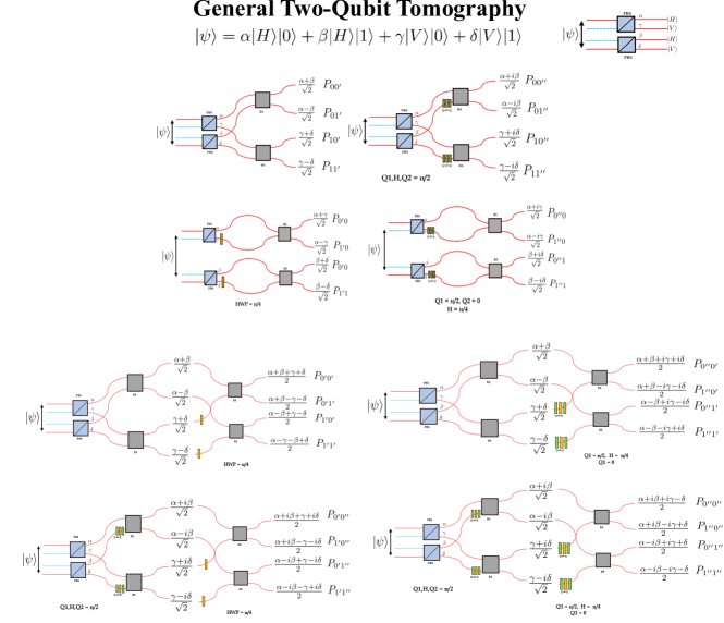
Figure 6: This figure outlines all the projection measurements necessary for reconstructing the density matrix of the 2-qubit system, along with the coefficients resulting from interference, are specified too. Additionally, it includes all the angles of the Q-H-Qs.

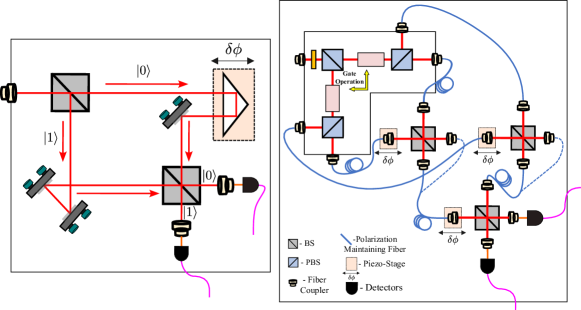
Figure 7: Full - 2 qubit tomography setup

Figure 8: Tomography of the relevant 2-qubit states and the fidelity mentioned in the table. More tomography figures for all gate operations are available upon request.

References

- [1] B. B. Blinov, D. Leibfried, C. Monroe and D. J. Wineland, Quantum Computing with Trapped Ion Hyperfine Qubits QIP, 3, 45 59, (2004).
- [2] D Jaksch, Optical lattices, ultracold atoms and quantum information processing Contemporary Physics 45, Issue 5, (2004).
- [3] John Clarke , Frank K Wilhelm, Superconducting quantum bits Nature 453, 1031-1042 (2008).
- [4] Stefanie Barz, Quantum computing with photons: introduction to the circuit model, the one-way quantum computer, and the fundamental principles of photonic experiments J. Phys. B: At. Mol. Opt. Phys. 48, 083001 (2015).
- [5] Christian Gross , Immanuel Bloch, Quantum simulations with ultracold atoms in optical lattices Science 357, 6355 (2017).
- [6] Frank Arute et. al, Quantum supremacy using a programmable superconducting processor Nature 574, 505 - 510 (2019).
- [7] Sergei Slussarenko , Geoff J. Pryde Photonic quantum information processing: A concise review Appl. Phys. Rev. 6, 041303 (2019).
- [8] Nicolás Quesada and Jonathan Lavoie et. al,Quantum computational advantage with a programmable photonic processor Nature 606, 75 - 81 (2022).
- [9] Jianwei Wang et. al, Very-large-scale integrated quantum graph photonics Nature Photonics, 17, 573 - 581(2023).
- [10] H. J. Briegel, D. E. Browne, W. Dür, R. Raussendorf & M. Van den Nest , Measurement-based quantum computation Nature Physics 5, 19 - 26 (2009).
- [11] Xi-Lin Wang et. al, 18-Qubit Entanglement with Six Photons’ Three Degrees of Freedom Phys. Rev. Lett. 120, 260502(2018).
- [12] Han-Sen Zhong et. al, Phase-Programmable Gaussian Boson Sampling Using Stimulated Squeezed Light Phys. Rev. Lett. 127, 180502 (2021).
- [13] E Knill 1, R Laflamme, G J Milburn, A scheme for efficient quantum computation with linear optics Nature 409, 46 - 52 (2001).
- [14] Jacob D. Biamonte and Peter J. Love, Realizable Hamiltonians for universal adiabatic quantum computers Phys. Rev. A 78, 012352 (2008).
- [15] Lilian Childress and Ronald Hanson, Diamond NV centers for quantum computing and quantum networks QIP, 38, pages 134 - 138, (2013).
- [16] N. Shenvi, J. Kempe, K. B. Whaley, Quantum random-walk search algorithm, Phys. Rev. A 67, 052307 (2003).
- [17] A. M. Childs, R. Cleve, E. Deotto, E. Farhi, et.al., Exponential algorithmic speedup by a quantum walk. Proceedings of the Thirty-fifth Annual ACM Symposium on Theory of Computing, 59 (2003).
- [18] Andris Ambainis, Quantum Walk and their Algorithmic Application International Journal of Quantum Information 01 ( 04), 507-518 (2003).
- [19] T. Oka, N. Konno, R. Arita,, H. Aoki, Breakdown of an electric-field driven system: a mapping to a quantum walk, Phys. Rev. Lett. 94, 100602 (2005).
- [20] F. W. Strauch, Relativistic quantum walks, Phys. Rev. A 73, 054302 (2006).
- [21] G. S. Engel, T. R. Calhoun, E. L. Read, T. -K, Ahn, et al. Evidence for wavelike energy transfer through quantum coherence in photosynthetic systems, Nature 446, 782 (2007).
- [22] M. Mohseni, P. Rebentrost, S. Lloyd, A. Aspuru-Guzik, Environment-assisted quantum walks in photosynthetic energy transfer, J. Chem. Phys. 129, 174106 (2008).
- [23] C. M. Chandrashekar, R. Laflamme, Quantum phase transition using quantum walks in an optical lattice, Phys. Rev. A 78, 022314 (2008).
- [24] T. Kitagawa, M. S. Rudner, E. Berg, E. Demler, Exploring topological phases with quantum walks, Phys. Rev. A 82, 033429 (2010).
- [25] C. M. Chandrashekar, Disordered-quantum-walk-induced localization of a Bose-Einstein condensate, Phys. Rev. A 83, 022320 (2011).
- [26] C. M. Chandrashekar, Two-component Dirac-like Hamiltonian for generating quantum walk on one-, two- and three-dimensional lattices, Sci. Rep. 3, 2829 (2013).
- [27] A. Mallick, C. M. Chandrashekar, Dirac cellular automaton from split-step quantum walk, Sci. Rep. 6, 25779 (2016).
- [28] A. Mallick, S. Mandal, C. M. Chandrashekar, Neutrino oscillations in discrete-time quantum walk framework,Eur. Phys. J. C 77, 85 (2017).
- [29] C. H. Alderete, S. Singh, N. H. Nguyen, et al., Quantum walks and Dirac cellular automata on a programmable trapped-ion quantum computer, Nat. Commun. 11, 3720 (2020).
- [30] A. Schreiber, K. N. Cassemiro, V. Potoek, A. Gabris, et al., Photons walking the line: a quantum walk with adjustable coin operations, Phys. Rev. Lett. 104, 050502 (2010).
- [31] Taira Giordani et. al, Experimental Engineering of Arbitrary Qudit States with Discrete-Time Quantum Walks. Phys. Rev. Lett. 122, 020503(2019).
- [32] M. A. Broome, A. Fedrizzi, B. P. Lanyon, I. Kassal, A. Aspuru-Guzik, and A. G. White, Discrete Single-Photon Quantum Walks with Tunable Decoherence Phys. Rev. Lett. 104, 153602(2010)
- [33] Youn-Chang Jeong, Carlo Di Franco, Hyang-Tag Lim, M.S. Kim and Yoon-Ho Kim, Experimental realization of a delayed-choice quantum walk Nature Communications 4 2471(2013)
- [34] A. Schreiber, K. N. Cassemiro, V. Potoček, A. Gábris, P. J. Mosley, E. Andersson, I. Jex, and Ch. Silberhorn, Photons Walking the Line: A Quantum Walk with Adjustable Coin Operations Phys. Rev. Lett. 104, 050502(2010)
- [35] Xiaogang Qiang , Thomas Loke , Ashley Montanaro , Kanin Aungskunsiri , Xiaoqi Zhou, Jeremy L O’Brien , Jingbo B Wang , Jonathan C F Matthews, Efficient quantum walk on a quantum processor Nature Communications vol.7, 11511(2016)
- [36] Schreiber, Andreas and Gábris, Aurél and Rohde, Peter P. and Laiho, Kaisa and Štefaňák, Martin and Potoček, Václav and Hamilton, Craig and Jex, Igor and Silberhorn, Christine, A 2D Quantum Walk Simulation of Two-Particle Dynamics, Science,336 6077(2012)
- [37] Pei Zhang, Bi-Heng Liu, Rui-Feng Liu, Hong-Rong Li, Fu-Li Li, and Guang-Can Guo, Implementation of one-dimensional quantum walks on spin-orbital angular momentum space of photons Phys. Rev. A 81, 052322(2010)
- [38] Farshad Nejadsattari, Yingwen Zhang, Frédéric Bouchard, Hugo Larocque, Alicia Sit, Eliahu Cohen, Robert Fickler, and Ebrahim Karimi, Experimental realization of wave-packet dynamics in cyclic quantum walks Optica Vol. 6, Issue 2, pp. 174-180 (2019)
- [39] Andrew M. Childs, Universal Computation by Quantum Walk Phys. Rev. Lett. 102, 180501(2009)
- [40] Neil B. Lovett, Sally Cooper, Matthew Everitt, Matthew Trevers, and Viv Kendon, Universal quantum computation using the discrete-time quantum walk Phys. Rev. A 81, 042330(2010)
- [41] Andrew M. Childs, David Gosset, Zak Webb, Universal Computation by Multi particle Quantum Walk Science Vol 339, Issue 6121(2013)
- [42] Shivani Singh, Prateek Chawla, Anupam Sarkar and C. M. Chandrashekar, Universal quantum computing using single-particle discrete-time quantum walk Scientific Reports V11,11551(2021)
- [43] Prateek Chawla, Shivani Singh, Aman Agarwal, Sarvesh Srinivasan and C. M. Chandrashekar, Multi-qubit quantum computing using discrete-time quantum walks on closed graphs Scientific Reports V13,12078(2023)
- [44] C. M. Chandrashekar, R. Srikanth, and Raymond Laflamme, Optimizing the discrete time quantum walk using a SU(2) coin Phys. Rev. A 82, 019902 (2010)
- [45] Salvador Elías Venegas-Andraca, Quantum walks: a comprehensive review QIP, 11, 1015–1106, (2012)
- [46] R. Simon, N. Mukunda, Minimal three-component SU(2) gadget for polarization optics Physics Letters A 143, 4, 5, (1990)
- [47] Sara Bartolucci et. al, Creation of Entangled Photonic States Using Linear Optics arXiv:2106.13825(2021)
- [48] P. Walther, K. J. Resch, T. Rudolph, E. Schenck, H. Weinfurter, V. Vedral, M. Aspelmeyer & A. Zeilinger, Nature volume 434, 169–176 (2005)