Towards a Generic Representation of Combinatorial Problems for Learning-Based Approaches

Abstract

In recent years, there has been a growing interest in using learning-based approaches for solving combinatorial problems, either in an end-to-end manner or in conjunction with traditional optimization algorithms. In both scenarios, the challenge lies in encoding the targeted combinatorial problems into a structure compatible with the learning algorithm. Many existing works have proposed problem-specific representations, often in the form of a graph, to leverage the advantages of graph neural networks. However, these approaches lack generality, as the representation cannot be easily transferred from one combinatorial problem to another one. While some attempts have been made to bridge this gap, they still offer a partial generality only. In response to this challenge, this paper advocates for progress toward a fully generic representation of combinatorial problems for learning-based approaches. The approach we propose involves constructing a graph by breaking down any constraint of a combinatorial problem into an abstract syntax tree and expressing relationships (e.g., a variable involved in a constraint) through the edges. Furthermore, we introduce a graph neural network architecture capable of efficiently learning from this representation. The tool provided operates on combinatorial problems expressed in the XCSP3 format, handling all the constraints available in the 2023 mini-track competition. Experimental results on four combinatorial problems demonstrate that our architecture achieves performance comparable to dedicated architectures while maintaining generality. Our code and trained models are publicly available at https://github.com/corail-research/learning-generic-csp.

1 Introduction

Combinatorial optimization has drawn the attention of computer scientists since the discipline emerged. Combinatorial problems, such as the traveling salesperson problem or the Boolean satisfiability have been the focus of many decades of research in the computer science community. We can now solve large problems of these kinds efficiently with exact methods [2] and heuristics [14]. Heuristics are handcrafted procedures that crystallize expert knowledge and intuition about the structure of the problems they are applied to. While heuristics have found success and applications for the resolution of combinatorial problems either as a direct-solving process or integrated into a search procedure, the rise of deep learning in many different fields [4, 7, 18, 24] has attracted the attention of researchers [5]. Among deep learning architectures, graph neural networks (GNNs) [29] have proven to be a powerful and flexible tool for solving combinatorial problems. However, as identified by Cappart et al. (2023) [8], it is still cumbersome to integrate GNN and machine learning into existing solving processes for practitioners. One reason is that a dedicated architecture must be designed and trained for each combinatorial problem. In addition to potentially expensive computing resources for training, this also requires the existence of a large and labeled training set.

Building such a problem-specific graph representation has been the preferred choice of most related approaches, such as NeuroSAT [30] leveraging an encoding for SAT formulas, or approaches tightly linked to the traveling salesperson problem [27, 16]. These approaches suffer from a lack of generality as the architecture could not be trivially exported from one combinatorial problem to another one (e.g., the representation in NeuroSAT cannot be used for encoding an instance of the traveling salesperson problem). Few attempts have been realized to bridge this gap, but they still provide only a partial genericity. For instance, Gasse et al. (2019) [13] proposed a bipartite graph linking variables and constraints when a variable is involved in a given constraint. However, this approach only encodes binary mixed-integer programs. Chalumeau et al. (2021) [10] later introduced a tripartite graph where variables, values, and constraints are specific types of vertices. This approach also lacks genericity as the method requires retraining when the number of variables changes. To our knowledge, the last attempt in this direction has been realized by Marty et al. (2023) [23] who leveraged a tripartite graph allowing decorating each vertex type with dedicated features. Although any combinatorial problem can theoretically be encoded with this framework, some information is lost with the encoding. For instance, it was not clear how the constraint $3x_{1}\leq 4x_{2}$, could be differentiated from the constraint $2x_{1}\leq 5x_{2}$. On the one hand, both constraints can be represented as an inequality, but we lose information about the variables’ coefficients. On the other hand, both constraints can be encoded as two distinct relationships, but in this case, we lose the fact that we have an inequality in both cases. More formally, their encoding function was not injective. Different instances could have the same encoding with no option to differentiate them. Besides, the experiments proposed only targeted relatively pure problems (maximum independent set, maximum cut, and graph coloring). Similar limitations are observed in the approach of Tönshoff et al. (2022) [31].

Based on this context, this paper progresses towards a fully generic representation of combinatorial problems for learning-based approaches. Intuitively, our idea is to break down any constraint of a problem instance as an abstract syntax tree and connect similar items (e.g., the same variables or constraints) through an edge. Then, we introduce a GNN architecture able to leverage this graph. To demonstrate the genericity of this approach, our architecture directly operates on instances expressed with the XCSP3 format [6] and can handle all the constraints available in the 2023 mini-track competition. Experiments are carried out on four problems (featuring standard intension, and global constraints such as allDifferent [28], table [11], negativeTable [33], element and sum) and aims to predict the satisfiability of the decision version of combinatorial problems. The results show that our generic architecture gives performances close to problem-specific architectures and outperforms the tripartite graph of Marty et al. (2023) [23].

2 Encoding Combinatorial Problem Instances as a Graph

Formally, a combinatorial problem instance $\mathcal{P}$ is defined as a tuple $\langle X,D(X),C,O\rangle$, where $X$ is the set of variables, $D(X)$ is the set of domains, $C$ is the set of constraints, and $O$ ($X\to\mathbb{R}$) is an objective function. A valid solution is an assignment of each variable to a value of its domain such that every constraint is satisfied. The optimal solution is a valid solution such that no other solution has a better value for the objective. Our goal is to build a function $\Phi:\langle X,D(X),C,O\rangle\mapsto\mathcal{G}(V,f,E)$, where $\mathcal{G}$ is a graph and $V$, $f$, $E$ are its vertex, vertex features and arc sets, respectively. We want this function to be injective, i.e., an encoding refers to at most one combinatorial problem instance. We propose to do so by introducing an encoding consisting in a heterogeneous and undirected graph featuring 5 types of vertices: variables (var), constraints (cst), values (val), operators (ope), and model (mod). The idea is to split each constraint as a sequence of elementary operations, to merge vertices representing the same variable or value, and connect together all the relationships. An illustration of this encoding is proposed in Figure 1 with a running example. Intuitively, this process is akin to building the abstract syntax tree of a program. Formally, the encoding gives a graph $\mathcal{G}(V,f,E)$ with $V=V_{\textsc{var}}\cup V_{\textsc{cst}}\cup V_{\textsc{val}}\cup V_{\textsc{ope}}\cup V_{\textsc{mod}}$ is a set containing the five types of vertices, $f=f_{\textsc{var}}\cup f_{\textsc{cst}}\cup f_{\textsc{val}}\cup f_{\textsc{ope}}\cup f_{\textsc{mod}}$ is the set of specific features attached to each vertex, and $E$ is the set of edges connecting vertices. Each type is defined as follows.

Values ($V_{\textsc{val}}$).

A value-vertex is introduced for each constant appearing in $\mathcal{P}$. Such values can appear inside either a domain or a constraint. All the values are distinct, i.e., they are represented by a unique vertex. The type of the value (integer, real, etc.) is added as a feature ($f_{\textsc{val}}$) to each value-vertex, using a one-hot encoding.

Variables ($V_{\textsc{var}}$).

A variable-vertex is introduced for each variable appearing in $\mathcal{P}$. A vertex related to a variable $x\in X$ is connected through an edge to each value $v$ inside the domain $D(x)$. Such as the value-vertices, all variables are represented by a unique vertex. The type of the variable (boolean, integer, set, etc.) is added as a feature ($f_{\textsc{var}}$) using a one-hot encoding.

Constraints ($V_{\textsc{cst}}$).

A constraint-vertex is introduced for each constraint appearing in $\mathcal{P}$. A vertex related to a constraint $c\in C$ is connected through an edge to each value $v$ that is present in the constraint. The type of the constraint (inequality, allDifferent, table, etc.) is added as a feature ($f_{\textsc{cst}}$) using a one-hot encoding.

Operators ($V_{\textsc{ope}}$).

Tightly related to constraints, operator-vertices are used to unveil the combinatorial structure of constraints. Specifically, operators represent modifications or restrictions on variables involved in constraints (e.g., arithmetic operators, logical operators, views, etc.). An operator-vertex is added each time a variable $x\in X$ is modified by such operations. The vertex is connected to the vertices related to the impacted variables. The type of the operator (+, $\times$, $\land$, $\lor$, etc.) is added as a feature ($f_{\textsc{ope}}$) using a one-hot encoding. If the operator uses a numerical value to modify a variable, this value is used as a feature ($f_{\textsc{ope}}$) as well.

Model ($V_{\textsc{mod}}$).

There is only one model-vertex per graph. This vertex is connected to all constraint-vertices and all variable-vertices involved in the objective function. Its semantics is to gather additional information about the instance (e.g., the direction of the optimization) by means of its feature vector ($f_{\textsc{mod}}$).

$$\mathsf{max}~{} x_{1}$$

$$\mathsf{s.t.}~{} 3x_{1}\leq 4x_{2}$$

$$\textsc{table}([x_{1},x_{2}],[(1,2),(2,3)])$$

$$x_{1}\in\{1,2\}$$

$$x_{2}\in\{2,3\}$$

Figure 1: Encoding of a combinatorial problem instance presented as a running example. There are $3$ value-vertices depicted (in green) and $2$ variable-vertices (in red). As $x_{1}$ contains values $1$ and $2$ in its domain, they are connected with an edge, and similarly for the domain of $x_{2}$. There are $2$ constraint-vertices (in blue), one for the inequality ($\leq$) and one for the table constraint (ext). The figure’s gray area illustrates the constraint $3x_{1}\leq 4x_{2}$, highlighted by operators (in orange) and showing a multiplication ($\times$, with feature $3$) of $x_{1}$ on the right-side (rhs) and another ($\times$, with feature $4$) of $x_{2}$ on the left-side (lhs). The rhs and lhs operators clarify equation sides, essential for distinguishing between $3x_{1}\leq 4x_{2}$ and $3x_{1}\geq 4x_{2}$, and link to the associated constraint (e.g., inequality $\leq$). The constraint $\textsc{table}([x_{1},x_{2}],[(1,2),(2,3)])$ is expressed in a similar way. It involves two tuples $t_{1}$ and $t_{2}$. Finally, the model-vertex (in yellow) is connected to the two constraints, and to variable $x_{1}$, as it is part of the objective function.

As a final remark, this encoding can be used to represent any combinatorial problem instance in a unique way. To do so, a parser for each constraint, describing how a constraint has to be split with the involved operators and variables, must be implemented. We currently support all the constraints formalized in XCSP3-core modeling format [6] and used for the mini-solver tracks of the XCSP-2023 competition: binary intension, table, negative table, short table, element and sum. Our repository contains the required documentation to build a graph from an instance in the XCSP3-core format with a description of all the features considered.

3 Learning from the Encoding with a Graph Neural Network

To achieve the next step and learn from this representation, we designed a tailored graph neural network (GNN) architecture to leverage this encoding. A GNN is a specialized neural architecture designed to compute a latent representation (known as an embedding) for each node of a given graph [29]. This process involves iteratively aggregating information from neighboring nodes. Each aggregation step is denoted as a layer of the GNN and incorporates learnable weights. There are various ways to perform this aggregation, leading to different variants of GNNs documented in the literature [20, 25, 32]. The model is differentiable and can then be trained with gradient descent methods.

Let $\mathcal{G}(V,f,E)$ be the graph encoding previously obtained, and let $h^{[i]}_{t,v}\in\mathbb{R}^{p}$ be a $p$-dimensional vector representation of a vertex $v\in V_{t}$ ($t$ refers to a vertex type from $\mathcal{T}:\{\textsc{var},\textsc{val},\textsc{cst},\textsc{ope},\textsc{mod}\}$) at iteration $i\in\{0,\ldots,I\}$. The inference process of a GNN consists in computing the next representations ($h^{[i+1]}_{t,v}$) from the previous ones for each vertex. This operation is commonly referred to as message passing. First, we set $h^{[0]}_{t,v}=f_{t,v}$ for each type, where $f_{t,v}$ is the vector of features related to vertex $v\in V_{t}$. Then, the representations at each iteration are obtained with LayerNorm [3] and LSTM layers [15]. The whole inference process is formalized in Algorithm 1. First, the initial embedding of each vertex is set to its feature (line 1) and the hidden states of the LSTM are initialized to 0 (line 1), as commonly done. Then, $I$ steps of message-passing are carried out (main loop). At each iteration $i$, a message ($\mu^{[i]}_{t_{1},v}$) is obtained for each vertex. The computation is done in three steps (line 1): (1) the embedding of each neighbor of a given type is summed up, (2) the resulting value is fed to a standard multi-layer perceptron ($\mathsf{MLP}^{\mathsf{in}}_{t_{1},t_{2}}$), note that there is a specific module for each edge type, (3) the messages related to each type are concatenated together ($\bigoplus$) to obtain the global message for each vertex. Notation $\mathcal{N}_{t_{2}}(v)$ refers to the set of neighbors of vertex $v$ of type $t_{2}$. The result is then given as input to an LSTM cell (line 1, one cell for each type) and is used to obtain the embedding at the next layer. We note that each LSTM has its internal state ($\gamma^{[i]}_{t,v}$) updated. At the end of the loop, each vertex has a specific embedding ($h^{[I]}_{t,v}$). After the last iteration, we compute the vertex-type dependent output by passing $h^{[I]}_{t,v}$ through a standard multi-layer perceptron $\mathsf{MLP}^{\mathsf{out}}_{t}$ (line 1). This produces the output embeddings for all nodes, which are then averaged (line 1). Finally, the sigmoid function ($\sigma$) is used to obtain an output between 0 and 1.

1 $\triangleright$ Pre: $\mathcal{G}(V_{\textsc{var},\textsc{cst},\textsc{val},\textsc{ope},\textsc{mod}},f_{\textsc{var},\textsc{cst},\textsc{val},\textsc{ope},\textsc{mod}},E)$ is the graph encoding.

2$\triangleright$ Pre: $\mathcal{T}:\{\textsc{var},\textsc{val},\textsc{cst},\textsc{ope},\textsc{mod}\}$ is the set of vertex-types.

3$\triangleright$ Pre: $I$ is the number of iterations of the GNN.

4 

5$h^{[0]}_{t,v}:=f_{t,v}~{}~{}~{}\forall v\in V_{t},\forall t\in\mathcal{T}$

6$\gamma^{[0]}_{t,v}:=0~{}~{}~{}~{}~{}~{}~{}~{}\forall v\in V_{t},\forall t\in\mathcal{T}$

7for $i~{}\mathbf{from}~{}1~{}\mathbf{to}~{}I$  do

8      

9      $\mu^{[i]}_{t_{1},v}:=\bigoplus\limits_{t_{2}\in\mathcal{T}}\mathsf{MLP}^{\mathsf{in}}_{t_{1},t_{2}}\Big{(}\sum\limits_{u\in\mathcal{N}_{t_{2}}(v)}h^{[i-1]}_{t_{2},u}\Big{)}~{}~{}~{}\forall v\in V_{t_{1}},\forall t_{1}\in\mathcal{T}$

10      $h^{[i]}_{t,v},\gamma^{[i]}_{t,v}:=\mathsf{LSTM}_{t}\Big{(}\mu^{[i]}_{t,v},\gamma^{[i-1]}_{t,v}\Big{)}~{}~{}~{}\forall v\in V_{t},\forall t\in\mathcal{T}$

11

12$\nu_{t,v}:=\mathsf{MLP}^{\mathsf{out}}_{t}\Big{(}h^{[I]}_{t,v}\Big{)}~{}~{}~{}\forall v\in V_{t},\forall t\in\mathcal{T}$

13$\hat{y}:=\sigma\Big{(}\frac{1}{|\mathcal{T}|\times|V|}\sum\limits_{t\in\mathcal{T}}\sum\limits_{v\in V_{t}}\nu_{t,v}\Big{)}$

14return $\hat{y}$

Algorithm 1 Inference process of our GNN architecture.

4 Experiments

This section evaluates our approach on combinatorial task, focusing on four problems: Boolean satisfiability (SAT), graph coloring (COL), knapsack (Knap), and the traveling salesperson problem (TSP) with TSP-Ext (table constraint) and TSP-Elem (element constraint) models. We trained models on the decision version of the problems, asking if a solution exists with costs under a target $k$. When there is no objective function, we have a plain constrained satisfaction problem (e.g., SAT). The aim is not to find the solution but to determine its existence, aligning with recent studies  [30, 27, 19, 21]. We compared our approach with problem-specific architectures and the tripartite graph of Marty et al. (2023)  [23]. For the latter, we extracted their graph representation and used it in our GNN. The evaluation metric considered is the accuracy in correctly predicting the answer to the decision problem. Details on experimental protocols and implementations follow.

Boolean Satisfiability.

Instances are generated with the random generator of Selsam et al. (2018) [30]. Briefly, the generator builds random pairs of SAT instances of $n$ variables by adding new random clauses until the problem becomes unsatisfiable. Once the problem becomes unsatisfiable, it changes the sign of the first literal of the problem, rendering it satisfiable. On average, clauses have an arity of 8. Both the satisfiable and unsatisfiable instances are included in the dataset. Still following Selsam et al. (2018), we built a dataset containing millions of instances having 10 to 40 literals. The SAT-dependent architecture considered in our analysis has been also introduced in the same paper. We used a training set of size 3,980,000 and a validation set of size 20,000.

Traveling Salesperson Problem.

Instances are generated with the random generator of Prates et al. (2018) [27]. The generation consists in (1) creating $n$ points in a $(\sqrt{2}/2\times\sqrt{2}/2)$ square, (2) building the distance matrix with the Euclidean distance, and (3) solving them using the Concorde solver [1] to obtain the optimal tour cost $C^{*}$. Two instances are then created: a feasible one and an unfeasible one with target costs of $1.02C^{*}$ and $0.98C^{*}$, respectively. We build two TSP models: a first one where the distance constraints are expressed with an extension constraint (TSP-Ext), and a second one with an element constraint (TSP-Elem). The motivation is to analyze the impact of the model on the resulting graph encoding and the performances. Still following Prates et al. (2018), we built the dataset with a number of cities $n$ sampled uniformly from $20$ to $40$. The TSP-dependent architecture considered in our analysis has been also introduced in the same paper. We used a training set of size 850,000 and a validation set of size 50,000.

Graph Coloring.

Instances are generated following Lemos et al. (2019) [19]. This generator builds graphs with 40 to 60 vertices. For each graph, a single edge is added such that the $k$-coloriability is altered. The instances are produced in pairs: one where the optimal value is $k$ and another one where it is higher. Our encoding leverages a standard model of the graph coloring featuring binary intension ($\neq$) constraints. The Col-dependent architecture has been also introduced in the same paper. We used a training set of size 140,000 and a validation set of size 10,000.

Knapsack.

We built instances containing 20 to 40 items and solved them to optimality to find the optimal value $V^{*}$. Then, we created two instances, a feasible one and an unfeasible one with a target cost of $1.02V^{*}$ and $0.98V^{*}$, respectively. Our encoding leverages a standard knapsack model featuring a sum constraint. The Knapsack-specific model was based on the model of Liu et al. (2020) [21]. We used a training set of size 950,000 and a validation set of size 50,000.

Implementation Details.

All models were trained with PyTorch [26] and PyTorch-Geometric [12] on a single Nvidia V100 32 GB GPU for up to 4 days or until convergence. We selected the model having the best performance on the validation set. To make the comparisons between specific and generic graphs fair, we trained all our models using a single GPU, and we tuned each model by varying the number of hidden units in the MLP and LSTM layers. Concerning the problem-specific architectures, we reused to same hyperparameters as described in their original publications. All models are trained with Adam optimizer [17] coupled with a learning rate scheduler and a weight decay of $10^{-8}$. The main hyperparameters used for our different models are detailed in the accompanying code. All our models are expressed using XCSP3 formalism. We implemented a parser to build the graph from this representation. Our code and trained models are publicly available.

4.1 Results: Accuracy of the Approaches

Table 1 summarizes the accuracy in predicting the correct answer on the validation set for each problem and baseline. Interestingly, we observe that our approach achieves similar or close performances as the problem-specific architectures for all the problems. We see it as a promising result, as our approach, thanks to its genericity, can be directly used for all the problems without designing a new dedicated architecture. On the other hand, the approach of Marty et al. (2023) [23], fails to achieve similar results except for the graph coloring. This is because this representation does not preserve the combinatorial structure of complex constraints (Col has only constraints like $x_{1}\neq x_{2}$).

Table 1: Prediction accuracy on holdout test set

Architecture	SAT	TSP-Ext	TSP-Elem	Col	Knap
Problem-specific	94.3%	96.3%		77.0 %	98.8%
Tripartite [23]	50.0%	50.0%		84.6%	50.0%
Ours	94.4%	84.5%	91.4%	84.4%	97.9%

While TSP-Elem achieves results close to the TSP-specific approach, TSP-Ext falls short significantly. This highlights the importance of using an appropriate combinatorial model for the encoding. Specifically, the encoding TSP-Elem has a size of $1841$ vertices and $13042$ edges, while TSP-Ext yields a graph of $5661$ vertices and $28322$ edges, for a same instance of 40 cities. This is consequently larger encoding, which is not desirable as it makes the model harder to train.

4.2 Analysis: Generalization to Larger Instances

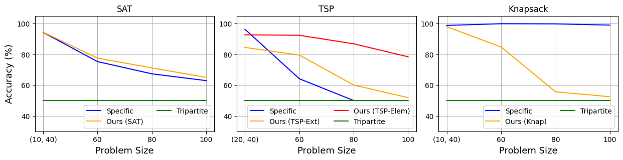
Figure 2: Analysis of the generalization ability on larger instances.

Figure 2 shows the generalization ability of the previous model, without retraining, on new instances with 60, 80 and 100 variables (5000 instances for each size). We observe that our generic representation provides a better generalization than the problem-specific architecture for SAT and TSP. Notably, TSP-Elem offers a far better generalization than TSP-Ext, confirming the impact of the input model and the size of the graph. Interestingly, we observe a strong generalization ability of the specific architecture for the knapsack. Our preliminary analysis indicates that this is achieved thanks to a GNN aggregation function based on a weighted sum. Understanding in detail the root causes of this generalization is part of our future work.

4.3 Discussion: Limitations and Challenges

Although the empirical results show the promise of this generic architecture, some limitations must be addressed. First, the training time required to obtain such results is prohibitive, although we have considered only relatively small instances so far. This is mainly because our encoding generates large graphs. This opens the door to integrating compression methods, dedicated to shrinking the size of the encoding without losing information. A parallel can be done with the smartTable [22] constraints, which encodes tables more compactly. It also highlights the importance of having a good input model, yielding a small embedding (e.g.,TSP-Elem versus TSP-Ext). Besides, the current task is restricted to solving the decision version of problems with an end-to-end approach. The next step will be to integrate this architecture in a full-fledged solver, such as what has been proposed by Gasse et al. (2019) for binary mixed-integer programs [13], and by Cappart et al. (2021) for constraint programming [9]. Finally, the generalization ability of a model trained for a specific problem (e.g., on the TSP) to a similar one (e.g., TSP with time windows) is an interesting aspect to investigate.

5 Conclusion and Perspectives

This paper introduced a first version of a generic procedure to encode arbitrary combinatorial problem instances into a graph for learning-based approaches. The encoding proposed is injective, meaning that each encoding can be obtained by only one instance. Besides, a tailored graph neural network has been proposed to learn from this encoding. Experimental results showed that our approach could achieve similar results as problem-specific architectures, without requiring the need to hand-craft a dedicated representation. All the constraints involved in the 2023 mini-track competition of XCSP3 are currently supported. Adding new constraints only requires the implementation of a parser. Our next steps are to challenge the approach on bigger and more complex problems, and on other combinatorial tasks (e.g., learning branching heuristics).

References

- [1] Applegate, D., Bixby, R., Chvatal, V., Cook, W.: Concorde TSP solver (2006)
- [2] Applegate, D.L., Bixby, R.E., Chvátal, V., Cook, W., Espinoza, D.G., Goycoolea, M., Helsgaun, K.: Certification of an optimal TSP tour through 85,900 cities. Operations Research Letters 37(1), 11–15 (Jan 2009). https://doi.org/10.1016/j.orl.2008.09.006
- [3] Ba, J.L., Kiros, J.R., Hinton, G.E.: Layer normalization. arXiv preprint arXiv:1607.06450 (2016)
- [4] Bahdanau, D., Cho, K.H., Bengio, Y.: Neural machine translation by jointly learning to align and translate. In: 3rd International Conference on Learning Representations, ICLR 2015 (2015)
- [5] Bengio, Y., Lodi, A., Prouvost, A.: Machine learning for combinatorial optimization: A methodological tour d’horizon. European Journal of Operational Research 290(2), 405–421 (2021). https://doi.org/https://doi.org/10.1016/j.ejor.2020.07.063
- [6] Boussemart, F., Lecoutre, C., Audemard, G., Piette, C.: XCSP3-core: A format for representing constraint satisfaction/optimization problems. arXiv preprint arXiv:2009.00514 (2020)
- [7] Brown, T., Mann, B., Ryder, N., Subbiah, M., Kaplan, J.D., Dhariwal, P., Neelakantan, A., Shyam, P., Sastry, G., Askell, A., et al.: Language models are few-shot learners. Advances in neural information processing systems 33, 1877–1901 (2020)
- [8] Cappart, Q., Chételat, D., Khalil, E.B., Lodi, A., Morris, C., Velickovic, P.: Combinatorial optimization and reasoning with graph neural networks. Journal of Machine Learning Research 24(130), 1–61 (2023)
- [9] Cappart, Q., Moisan, T., Rousseau, L.M., Prémont-Schwarz, I., Cire, A.A.: Combining reinforcement learning and constraint programming for combinatorial optimization. In: Proceedings of the AAAI Conference on Artificial Intelligence. vol. 35, pp. 3677–3687 (2021)
- [10] Chalumeau, F., Coulon, I., Cappart, Q., Rousseau, L.M.: Seapearl: A constraint programming solver guided by reinforcement learning. In: Integration of Constraint Programming, Artificial Intelligence, and Operations Research: 18th International Conference, CPAIOR 2021, Vienna, Austria, July 5–8, 2021, Proceedings 18. pp. 392–409. Springer (2021)
- [11] Demeulenaere, J., Hartert, R., Lecoutre, C., Perez, G., Perron, L., Régin, J.C., Schaus, P.: Compact-table: efficiently filtering table constraints with reversible sparse bit-sets. In: Principles and Practice of Constraint Programming: 22nd International Conference, CP 2016, Toulouse, France, September 5-9, 2016, Proceedings 22. pp. 207–223. Springer (2016)
- [12] Fey, M., Lenssen, J.E.: Fast graph representation learning with PyTorch Geometric. In: ICLR Workshop on Representation Learning on Graphs and Manifolds (2019)
- [13] Gasse, M., Chételat, D., Ferroni, N., Charlin, L., Lodi, A.: Exact combinatorial optimization with graph convolutional neural networks. vol. 32 (2019)
- [14] Helsgaun, K.: An Extension of the Lin-Kernighan-Helsgaun TSP Solver for Constrained Traveling Salesman and Vehicle Routing Problems: Technical report. Roskilde Universitet (Dec 2017)
- [15] Hochreiter, S., Schmidhuber, J.: Long short-term memory. Neural computation 9(8), 1735–1780 (1997)
- [16] Joshi, C.K., Cappart, Q., Rousseau, L.M., Laurent, T.: Learning the travelling salesperson problem requires rethinking generalization. Constraints 27(1-2), 70–98 (2022)
- [17] Kingma, D.P., Ba, J.: Adam: A method for stochastic optimization. arXiv preprint arXiv:1412.6980 (2014)
- [18] Krizhevsky, A., Sutskever, I., Hinton, G.E.: Imagenet classification with deep convolutional neural networks. Advances in neural information processing systems 25 (2012)
- [19] Lemos, H., Prates, M., Avelar, P., Lamb, L.: Graph colouring meets deep learning: Effective graph neural network models for combinatorial problems. In: 2019 IEEE 31st International Conference on Tools with Artificial Intelligence (ICTAI). pp. 879–885. IEEE (2019)
- [20] Li, Y., Zemel, R., Brockschmidt, M., Tarlow, D.: Gated graph sequence neural networks. In: International Conference on Learning Representations (2016)
- [21] Liu, M., Zhang, F., Huang, P., Niu, S., Ma, F., Zhang, J.: Learning the satisfiability of pseudo-boolean problem with graph neural networks. In: Principles and Practice of Constraint Programming: 26th International Conference, CP 2020, Louvain-la-Neuve, Belgium, September 7–11, 2020, Proceedings 26. pp. 885–898. Springer (2020)
- [22] Mairy, J.B., Deville, Y., Lecoutre, C.: The smart table constraint. In: Integration of AI and OR Techniques in Constraint Programming: 12th International Conference, CPAIOR 2015, Barcelona, Spain, May 18-22, 2015, Proceedings 12. pp. 271–287. Springer (2015)
- [23] Marty, T., François, T., Tessier, P., Gautier, L., Rousseau, L.M., Cappart, Q.: Learning a generic value-selection heuristic inside a constraint programming solver. In: 29th International Conference on Principles and Practice of Constraint Programming (2023)
- [24] Mnih, V., Kavukcuoglu, K., Silver, D., Rusu, A.A., Veness, J., Bellemare, M.G., Graves, A., Riedmiller, M., Fidjeland, A.K., Ostrovski, G., et al.: Human-level control through deep reinforcement learning. nature 518(7540), 529–533 (2015)
- [25] Monti, F., Boscaini, D., Masci, J., Rodola, E., Svoboda, J., Bronstein, M.M.: Geometric deep learning on graphs and manifolds using mixture model CNNs. In: Proceedings of the IEEE conference on computer vision and pattern recognition. pp. 5115–5124 (2017)
- [26] Paszke, A., Gross, S., Massa, F., Lerer, A., Bradbury, J., Chanan, G., Killeen, T., Lin, Z., Gimelshein, N., Antiga, L., et al.: Pytorch: An imperative style, high-performance deep learning library. Advances in neural information processing systems 32 (2019)
- [27] Prates, M., Avelar, P.H., Lemos, H., Lamb, L.C., Vardi, M.Y.: Learning to solve np-complete problems: A graph neural network for decision TSP. In: Proceedings of the AAAI Conference on Artificial Intelligence. vol. 33, pp. 4731–4738 (2019)
- [28] Régin, J.C.: A filtering algorithm for constraints of difference in CSPs. In: AAAI. vol. 94, pp. 362–367 (1994)
- [29] Scarselli, F., Gori, M., Tsoi, A.C., Hagenbuchner, M., Monfardini, G.: The graph neural network model. IEEE transactions on neural networks 20(1), 61–80 (2008)
- [30] Selsam, D., Lamm, M., Bünz, B., Liang, P., de Moura, L., Dill, D.L.: Learning a SAT solver from single-bit supervision. In: International Conference on Learning Representations (2019)
- [31] Tönshoff, J., Kisin, B., Lindner, J., Grohe, M.: One model, any CSP: Graph neural networks as fast global search heuristics for constraint satisfaction. arXiv preprint arXiv:2208.10227 (2022)
- [32] Veličković, P., Cucurull, G., Casanova, A., Romero, A., Liò, P., Bengio, Y.: Graph attention networks. In: International Conference on Learning Representations (2018)
- [33] Verhaeghe, H., Lecoutre, C., Schaus, P.: Extending compact-table to negative and short tables. In: Proceedings of the AAAI Conference on Artificial Intelligence. vol. 31 (2017)