CarbonNet: How Computer Vision Plays a Role in Climate Change?
Application: Learning Geomechanics from Subsurface Geometry of CCS to Mitigate Global Warming

Abstract

We introduce a new approach using computer vision to predict the land surface displacement from subsurface geometry images for Carbon Capture and Sequestration (CCS). CCS has been proved to be a key component for a carbon neutral society. However, scientists see there are challenges along the way including the high computational cost due to the large model scale and limitations to generalize a pre-trained model with complex physics. We tackle those challenges by training models directly from the subsurface geometry images. The goal is to understand the respons of land surface displacement due to carbon injection and utilize our trained models to inform decision making in CCS projects.

We implement multiple models (CNN, ResNet, and ResNetUNet) for static mechanics problem, which is a image prediction problem. Next, we use the LSTM and transformer for transient mechanics scenario, which is a video prediction problem. It shows ResNetUNet outperforms the others thanks to its architecture in static mechanics problem, and LSTM shows comparable performance to transformer in transient problem. This report proceeds by outlining our dataset in detail followed by model descriptions in method section. Result and discussion state the key learning, observations, and conclusion with future work rounds out the paper.

1 Introduction

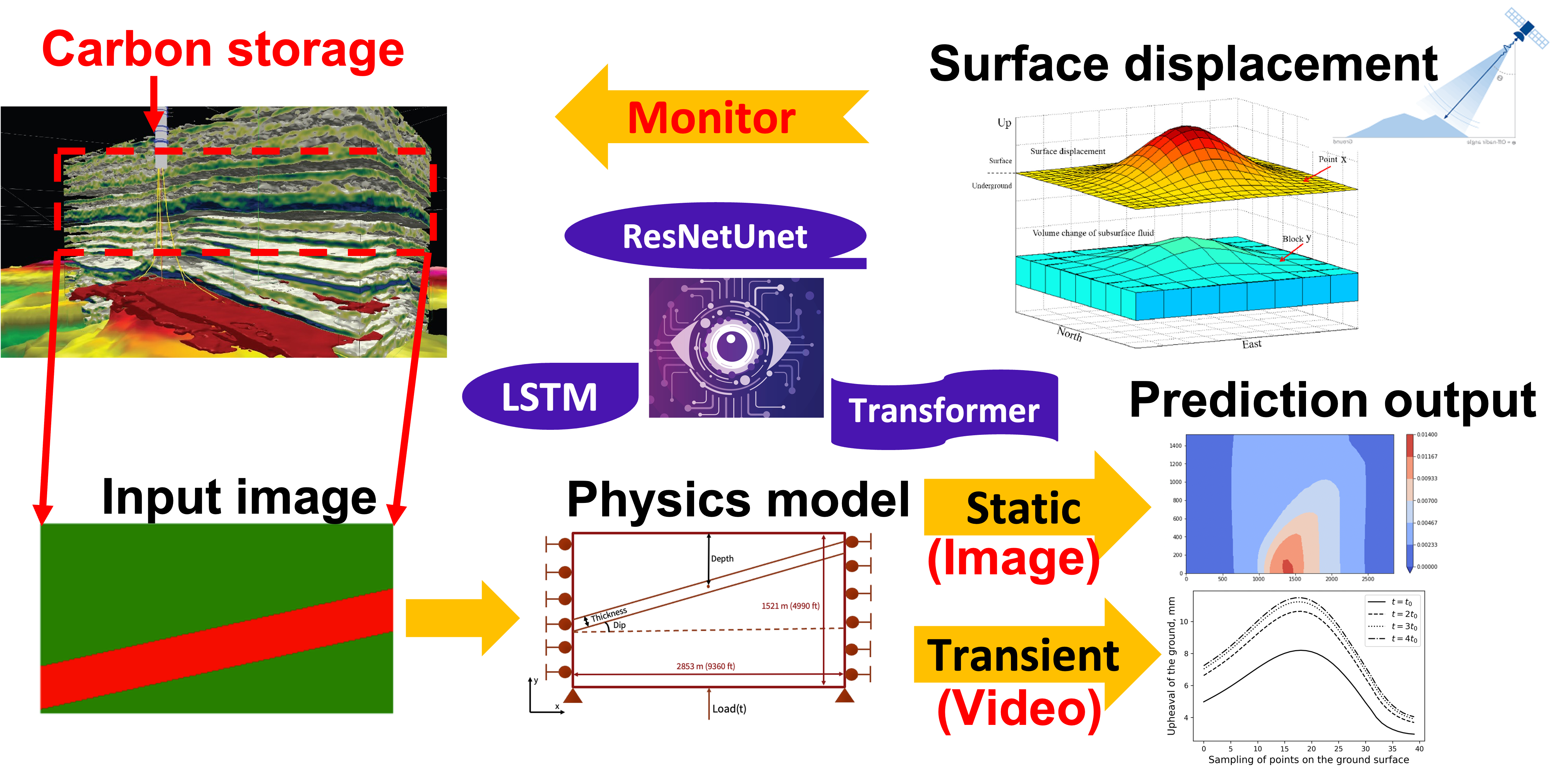
Figure 1: A summary of workflow of this project, and the goal is to leverage computer vision intelligence for carbon storage surveillance in order to mitigate climate change. ResNetUnet assists the image prediction in terms of land surface displacement, and we use LSTM and transformer to predict displacement change over time, that is a video problem in computer vision domain.

CCS is an important emissions reduction technology to alleviate global warming and climate changestephens2006growing . In CCS, the supercritical $CO_{2}$ is injected into the deep brine aquifers or abandoned oil reservoirs for permanent storage. However, the possible risk is the surface upheaval induced by excessive fluid pressure, which is possible to damage the structures on the ground and influence people’s lives li2013application . Understanding and predicting the spatial distribution and temporal change of surface deformation is important to avoid the possible hazards. However, its realization is challenged by the large spatial scale and long time scale of the project, which makes the direct numerical simulation computationally prohibitive. As the traditional numerical simulation usually requires extensive computing resourcesVilarrasa2010 ; Shi2013 ; Li2016 ; Fuchs2019 ; Talebian2013 , the neural networks may provide a less accurate, but more efficient and sufficient solution beneficial for the model-based decision making and planning Tang2021 . We formulate the entire project as the workflow described in Fig. 1. The project is to predict the variation of surface vertical displacement (upheaval) with time induced by injected fluid under different subsurface geometry settings. The input are 2D images of subsurface geometry consisting of a shale layer embedded with different dip angles in two permeable layers. The output is the displacement image. The shale layer and permeable layer have large contrast in their mechanical property as stiffness $\mathbb{C}^{e}$ and flow property as permeability $\boldsymbol{\kappa}$ josh2012laboratory .

In this project, we are motivated to apply deep learning models to predict the land surface displacement under different subsurface geometries in a coupled geomechanics and flow problem. We start from the static mechanics model, where the fluid pressure is treated as the prescribed traction boundary conditions. For prediction in terms of the static mechanics model, the input to our algorithm is a geometry image. We then use different models (CNN, ResNet, ResNetUNet) to output a predicted displacement image (Fig. 1 static prediction output) across the domain of input geometry image. ResNetUNet is designed by us to combine the advantages of UNet and ResNet architecture to map different subsurface geometries to the distribution of the 2D displacement field.

From the ResNetUNet in static mechanics model, we continue to the LSTM and transformer model to predict the temporal change of surface displacement. The input to our algorithm is a geometry image along with five frames of displacement curves, which is in format of a short video. We then use LSTM and transformer to output predicted displacement curve (Fig. 1 transient prediction output) at the next time step. LSTM is a typical algorithm for time series predictions, and we are motivated to test transformer because of its self-attention mechanism. It provides the possibility to predict the long term dependency by contracting any two locations to a constant, so that it overcomes the issue of information loss in sequence computing in LSTM zeyer2019comparison .

2 Related Work

Deep learning approaches have been proved to be effective on predicting the static and time-dependent dynamics of a system under the governing physics principles as partial differential equations (PDE). The current existing deep learning approaches are of two types as physics-based neural networks (PINN) Xu2020 ; Meng2020 ; Zheng2020 and the simulation data driven approachesTang2021 ; Tang2020 ; Wen2021 ; nie2020stress . The difference is whether the direct simulation data is needed to train the model.

PINN method obtains the approximate solution by minimizing the residual in physics governing equations. In contrast, common numerical discretization methods use finite difference method (FDM) and finite element method (FEM). PINN is a mesh-free method to employ automatic differentiation to handle differential operators. The existing PINN model for coupled flow and geomechanics problembekele2020deep is limited to one dimensional problem, and it ignores the influence of material heterogeneity. Besides, it only predicts the excess pore pressure in flow side, but not the surface displacement from geomechanics side. The other type of deep learning approaches is simulation data driven method, which takes the solution from simulation directly as training data. The end-to-end image based approaches take both input and output, from figures with the model geometry as input to the contour plot showing the distribution of different physical quantities (fluid pressure, displacement) as output. The ResNet CNN was applied to predict stress field of a 2D cantilever beam under different boundary conditions nie2020stress . Nevertheless, it is limited to static solid mechanics problem ignoring the coupling between fluid flow and mechanics response. Besides, it only deals with homogeneous model, which is not the case in reality. The R-U-Net model with LSTM is used to predict the temporal and spatial distribution of surface displacement Tang2021 , fluid pressure and saturation in the 3D model. However, it is restricted to predict one specific geological formation setting.

In order to predict the temporal change of the surface displacement under different geological formation settings, a more advanced model is needed to capture the dynamics changing with time. Transformer and self-attention models NIPS2017_3f5ee243 , which were originally developed in NLP, shows its ability to outperform other methods by learning longer-term dependencies without recurrent connections. Transformer has been used to predict the representative dynamical systems such as 2D fluid dynamics and 3D reaction-diffusion dynamics nie2020stress . The model shows its effectiveness to capture the varying behavior of different physical phenomenon evolution. Therefore, transformer is chosen to predict the transient behavior of surface displacement under different subsurface geometry setting in our project as well.

3 Dataset

In the section, we demonstrate the dataset used in the project. The dataset includes two parts as the static model and the transient model. The input dataset are 2D geometries of geological layers (Fig. 1 input image), which consists of two heterogeneous materials as the hard rock with high permeability and soft shale with low permeability; and the label is surface displacement contour (Fig. 1 static prediction output image) under specific loading. The geometries are sampled according to the real underground stratum. The size of the domain (length and width of the rectangle), the thickness, and the depth of shale layer is fixed, while the variable is the dip angle of shale layer. The data of surface displacement field is generated from simulation results in FEniCS (an open-source computational platform using Finite element Method (FEM)) alnaes2015fenics . The model setting used in the problem is depicted in Fig. 2. Data augmentation is not necessary in the project because we could generate as many training samples as we want from the physics simulation.

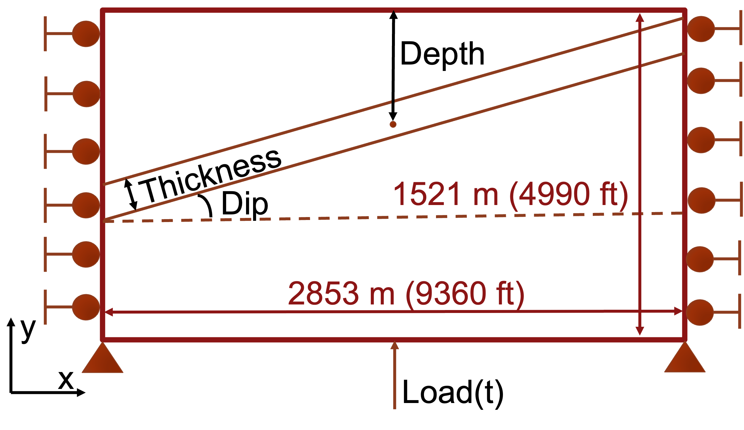
Figure 2: The layout of the computational problem. The end of the computational program is to capture the displacement given the configuration of the loading, material distribution and boundary conditionsbathe2007finite .

3.0.1 Geometry as the input

The geometries are generated as the input of machine learning model by PIL.draw modulus, and are depicted in the Fig. 1, labeled as input image. The material characteristics of the shale and rock are distinct, thus different layout of the material will yield different results. We generate 10000 groups of data by sampling the dip angles from 0^∘ to 45^∘ uniformly for the training purpose. Different dip angles correspond to specific geometries, which impact the result of displacement.We split the entire dataset with 95% for training and 5% for validation. Next, we generated 5% of new samples for testing.

3.0.2 Static displacement as the label

We consider vertical displacement $u_{y}$ as the label, which is defined on each vertices of the finite element mesh ho1988finite , and can be considered as the displacement at points uniformly sampled over the domain. The vertical displacement ($u_{y}$) corresponds to the upheaval of the stratum. The FEniCS program provides the following API:

$$\text{Layout of problem}\Longrightarrow\text{$u_{y}$ across the domain}$$ (1)

As for the labels (ground truth), we use a numpy 1D array to store the vertical displacement of 1250 points from a uniform $50\times 25$ points sampled over the domain. The dataset is demonstrated in Tab. 1.

For the mathematical interpretation, refer to the Appendix A.

Table 1: The dataset for the static machine learning model.

input image	groundtruth/label
Input image with dip angle 0	numpy array (1250 size)
$\vdots$    (9998 examples)	$\vdots$    (9998 examples)
Input image with dip angle $45^{\circ}$	numpy array (1250 size)

3.0.3 Transient displacement as the label

Based on the static model, the next problem we deal with is the coupled hydro-mechanical simulation, which takes the pressure of fluid into account to better simulate the real situation. The coupled hydro-mechanical simulation is widely applied in the industry, and is well-known for dealing with consolidation case, which is a transient (time-dependent) problems. We use the same kind of geometry as what we generated for the static case, but employ another set of equations to simulate the physics process. The mathematical interpretation can be found in Appendix A.

In the static case, we calculate one step of displacement across the domain, given one input geometry. However, the transient simulation will yield multiple images at different time steps given one single geometry. In addition, we focus on the vertical displacement on the ground, which is the interest in industry. In this project, we sample 40 points on the ground surface, and capture their vertical displacement.

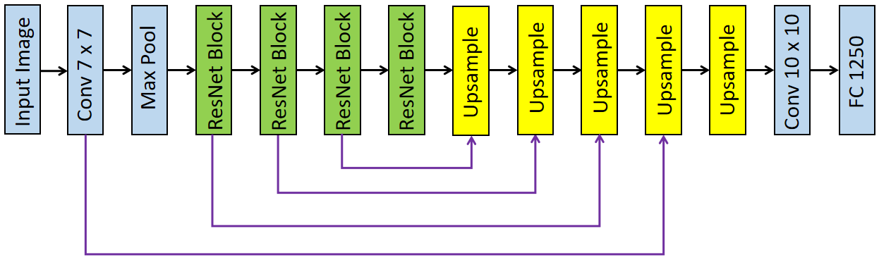
Figure 3: The architecture of ResetNetUnet, designed by ourselves for the displacement prediction of heterogeneous computational mechanics problem. The detail of the architecture is provided in the supplement section.

The dataset is illustrated in Tab. 2.

Table 2: The dataset for the transient machine learning model.

input image	ground truth/label
Input image with dip angle 0	1000 time steps
	of numpy array (40 size)
$\vdots$    (2998 examples)	$\vdots$    (2998 examples)
Input image with dip angle 0	1000 time steps
	of numpy array (40 size)

To further prepare the data for the time series prediction model, we conduct the min-max scaling for the data by

$$X=\frac{X-X_{\min}}{X_{\max}-X_{\min}}.$$ (2)

Also, we create the data sequence for the transformer and LSTM model later by using continuous five data points to predict the next data point, like

$$u_{y,t},u_{y,t+1},u_{y,t+2},u_{y,t+3},u_{y,t+4}\Longrightarrow u_{y,t+5},$$ (3)

where each $u_{y,t}$ represents a 1D array with size of 40. We adopt sliding windows to generate the sequence, thus generating $89400$ pieces of displacement sequence. Similarly, we split the dataset with 95% for training, 5% for validation, and generate new samples (5%) for testing.

4 Methods

In this project, we deal with two different computational problems, the static mechanics and the transient mechanics. We developed three models, which includes a well-designed combination of ResNet and UNet model to predict the static displacement, and the LSTM and transformer model that base on the pretrained ResNetUNet model.

4.1 Static mechanics model

We are motivated to start from CNN models by literature nie2020stress , and further test ResNet and UNet from a similar deep learning problem to handle heterogeneity in input images charng2020deep . The CNN and ResNet network reduces the dimension of images layer by layer. It loses information while collecting important features from input. Meanwhile, the deep neural network constructed by the ResNet can be utilized to decode the physical Eq. 6, which is a complicated procedure. Additionally, the heterogeneous distribution of material impacts the final result considerably. Inspired by the segmentation in computer vision ronneberger2015u , we use UNet to capture the heterogeneous distribution of the pixel/material.

4.1.1 Baseline model: CNN and Resnet

As the baseline model, we use the most basic CNN model, using continuous layers of convolution blocks which comprises a conv2d, BatchNorm2d and relu. Finally, we flatten the convolution to get a fully connected layer with 1250 dimensions for output. For the other baseline model, ResNet, we use the resnet18 model in Pytorch and modify the last layer to have the convolution with width, height and channel as $50\times 25\times 1$, which will be flattened as the fully connected layer afterwords.

4.1.2 Model: ResNetUNet

ResNetUNet is the model designed by ourselves to solve the current problem. Compared to the conventional UNet ronneberger2015u , we modify the encoder part by using the ResNet for downsampling the image to better capture the physical equations. The upsampling is the same as the traditional UNet zhou2019d . The architecture of the ResNetUNet is illustrated in the Fig. 3. The special part here is the residual block, which replace the ordinary CNN layer in UNet with two consecutive residual blocks, as is shown in Fig. 4. To successfully fulfill the functionality, we need to capture both the heterogeneous features and the physics equations laws. The UNet part is to do a segmentation-like work to distinguish the shale and rock, while the ResNet part is to learn the complicated physics laws.

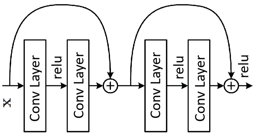
Figure 4: The implementation of the ResNet block in the ResNetUNet architecture.

As for the loss function, we adopt the mean square error (MSE) for all the three models above.

$$\text{MSE}(y,\hat{y})=\sum_{i=1}^{m}\frac{(y_{i}-\hat{y}_{i})^{2}}{m},$$ (4)

where $m$ is the number of examples. Note that we use the MSE for the loss function, but use both MSE and maximum absolute error (MAE) for the evaluation metrics.

$$\text{MAE}(y,\hat{y})=\sum_{i=1}^{m}\frac{|y_{i}-\hat{y}_{i}|}{m},$$ (5)

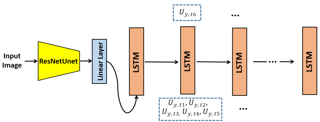
Figure 5: The architecture of the LSTM model to predict the evolution of vertical displacement.

4.2 Transient mechanics model

In this part, we use both the LSTM and transformer to predict the evolution of vertical displacement, the interest in industry, given the specified material distribution as an image. We adopt two models, LSTM and transformer, to perform the task, which is similar to an image caption work tan2019phrase ; liu2021cptr , except that we use the displacement as the sequence rather than the words embedding.

4.2.1 LSTM model

The combination of CNN and LSTM have been proved effective for the image caption work tan2019phrase . The CNN can be used to extract the features of the input image to feed into the LSTM network flow together with the sequence to be processed. In this project, we use a pretrained model in the static case to process the input geometry to get the features, which can embody the heterogeneous distribution of the material. The pretrained model used here is the ResNetUNet model trained in the static case, which has been proved effective for the feature extraction. Then, we add a linear layer for enhancing expressivity of the model, and processing the features further to enter the LSTM network. The linear layer has the architecture of in_features=1250, and out_feature=40.

For LSTM model, we use five steps of data points as the input to predict the next single step. Since the dimension of the sequence is 40, the number of points sampled on the ground surface, thus, we use the input size of the sequence as 40. The LSTMCell model, which includes input modulation gate, input gate, forget gate and output gate braun2018lstm , in Pytorch is adopted, and it is initialized by setting the input size as 40, and the hidden size as 4. We stack four LSTMCells to construct the model. The main architecture is depicted in Fig. 5. The loss function used in this model is MSE, which is the same as the Eq. 4. Also, we use both MSE and MAE as the metrics to evaluate the model.

The architecture of this model is inspired by the image caption model of LSTM soh2016learning . The difference lies in that we use the continuous value of the displacement as the data, rather than the softmax classification of the word embedding. Thus, the loss function for the two tasks is also distinct. Based on the accuracy requirements from the industry, the dimensions of the sequence data in our engineering application are approximately the same as the dimensions of words in natural language processing. The similarity in the two models provides the confidence to build the machine learning model based on the image caption model in NLP.

4.2.2 Transformer model

For the transformer model, we use the pretrained ResNetUNet to extract the image features as well, and feed it into a linear layer for secondary process. The output of the linear layer then enters the transformer encoder. As for the decoder input, we use five consecutive sequences as the input and the next five consecutive sequences as the output. For example, we use $u_{y,t_{1}},u_{y,t_{2}},u_{y,t_{3}},u_{y,t_{4}},u_{y,t_{5}}$ as the input to predict the output as $u_{y,t_{2}},u_{y,t_{3}},u_{y,t_{4}},u_{y,t_{5}},u_{y,t_{6}}$.

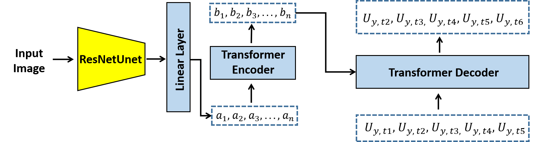
Figure 6: The architecture of the transformer model to predict the evolution of vertical displacement.

The input linear layer here has input features with size 1250, and out features with size 40, which reduces the dimensions of the output of pretrained model to 40. For the encoder part, we design another linear layer to convert the dimension from 40 to 16 to optimize the memory. The output then enters the positional encoding layer to take the order of the sequence into account. Then, we employ the nn.TransformerEncoderLayer in the Pytorch to assemble the encoder. The structure of the encoder is standardized from the attention paper vaswani2017attention . The parameters we set for the encoder layer are d_model=16, nhead= 8. We stack four nn.TransformerEncoderLayer to form the encoder layer. For decoder, we use nn.TransformerDecoderLayer, which have the structure of d_model=16, nhead= 8. And we stack four of them to set up the decoder layer. At the end of the transformer layer, we add a linear mapping to map the dimension inner the decoder to the sequence dimension. The main architecture of the transformer is illustrated in Fig. 6.

5 Results

We have studied a baseline model to predict the displacement images based on the static mechanics model. The baseline models (CNN and ResNet) are compared to a ResNetUNet model for discussion. Next, we implemented LSTM and transformer as two different models for transient mechanics model, because this is a problem related to videos. The deep learning model prediction is compared with physics modeling result, that is treated as the ground truth in this project. Due to the sufficient amount of training samples, we do not include cross validation in this work.

5.1 Static mechanics model

We selected CNN as a baseline model because it collects important information from input images as features by filtering through all pixels. We have found the different subsurface geometry has strong correlation to the displacement images, and that motivates us to try CNN first to examine its performance. We generated a total of 10,000 samples and then selected 95% for training and 5% for validation. The mini batch size is 32 because this fits our CPU/GPU memory, and we prioritize the model convergence speed for less number of epochs. Although a smaller mini batch size could be less efficient in gradient calculation terms bengio2012practical , a large batch may degrade the quality of the model because it tends to converge to sharp minima keskar2016large . We tuned the hyperparameters including learning rate, optimizer, beta1, beta2, and weight decay to expect decrease of validation loss values versus the number of epochs. We also compare the training loss versus validation loss to avoid underfitting or overfitting problems. Therefore, the learning is tuned to be 5e-6, and the weight decay is 1e-5. We finally use Adam as our optimizer, because it requires less memory with large number of parameters. More importantly, the hyperparameters have intuitive interpretation, and it requires less tuning with low computational costs kingma2014adam .

ResNet is the second model we investigated for static mechanics model prediction. The motivation for ResNet is high accuracy with moderate efficiency. It has deeper neural network structure so that it is capable to express more complex models. We set the same mini batch size as well as the number of epochs for training, and we follow a similar procedure to determine the hyperparameters, including learning rate, beta1, beta2, weight decay, and so on. The training loss and validation loss change versus epochs helps to determine the hyperparameters.

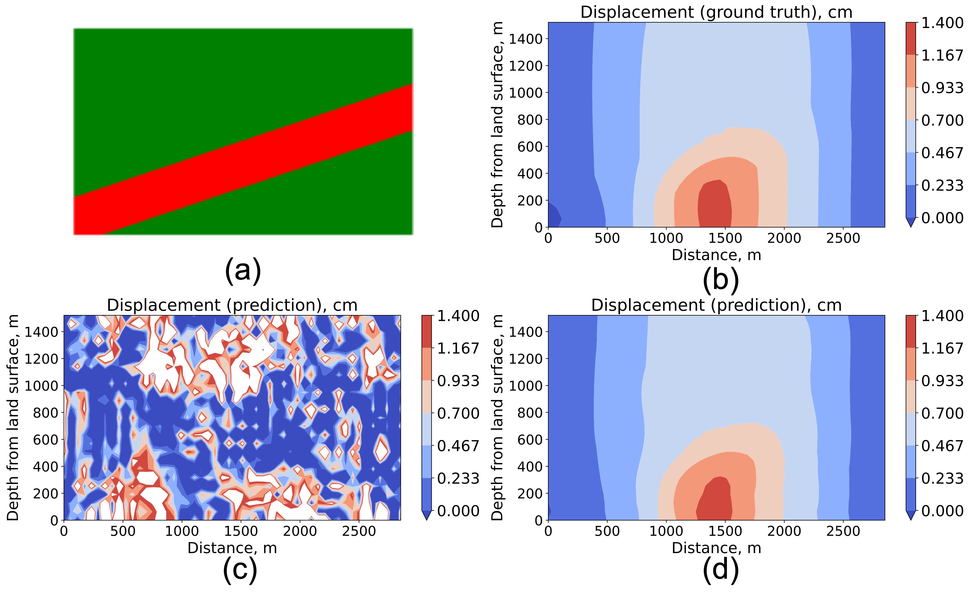
Figure 7: Comparison of ResNet and ResNetUNet prediction of the displacement images based on the geometry image as input. (a) is the input image for deep learning models, (b) is the ground truth based on physics, (c) is the prediction from our trained ResNet model and (d) is the prediction from ResNetUNet model.

The goal in this part is to develop a deep learning model to accurately predict the displacement images. Therefore, it is important to visually see the predictions versus ground truth side by side. Figure 7 shows the comparison of performance based on different models. The color represents different values of displacement as a physical parameter according to the color bar, and the unit is in meter. From the ground truth image (Fig. 7 (b)), we observe the largest displacement happens close to the point where we apply the load. And the displacement change is getting smaller when getting farther away from the point with an applied stress. The reason to see this contour is not symmetric is that we consider heterogeneity in this system. This means the material of the subsurface rock is not the same at all different locations. The motivation comes from the subsurface engineers to characterize cases that could better represent the real world scenarios. Our ResNet prediction (Fig. 7 (c)) illustrates a general trend of the displacement image on the right side of the Fig. 7. However, it clearly shows the prediction is not sufficient for accurate predictions. The result from CNN model shows comparable observations, therefore, we decide to use one failed case for analysis here. The reason is that ResNet and CNN downsamples from the input image to extract features, at the same time, the information loss through this process leads to the small regions not having values in Fig. 7 (c).

It is motivated to further improve the work by introducing ResNetUNet model because UNet includes an upsampling procedure that includes all information from each step of the downsampling process. This tends to avoid the information loss and provide more accurate predictions. We follow the same design of mini batch as well as the selection of optimizer to be Adam for this new model. And the same criterion is applied to determine hyperparameters including learning rate, beta1, beta2, and weight decay.

We tuned the learning rate to be 2e-6 in order to be sufficient. And we kept the other hyperparameters the same as CNN and ResNet models. Figure 7 (d) illustrates our results from the prediction based on ResNetUNet model. We clearly observe the significant improvement in terms of the predictions. The images are almost the same as each other and the values are comparable, which is represented by the color of contours in those images. The functionality of the ResNetUNet can be delved deeper by extract the intermediate features along the network flow as depicted in Fig. 8. The four ResNet blocks are critical to capture the features of the image. We can observe that the heterogeneity of the input geometry is captured first, and the pixel begins to spread and oscillate, which is due to the physics that we need to learn. At the last ResNet block, all the information is compressed to be unsampled by the decoder part of the network.

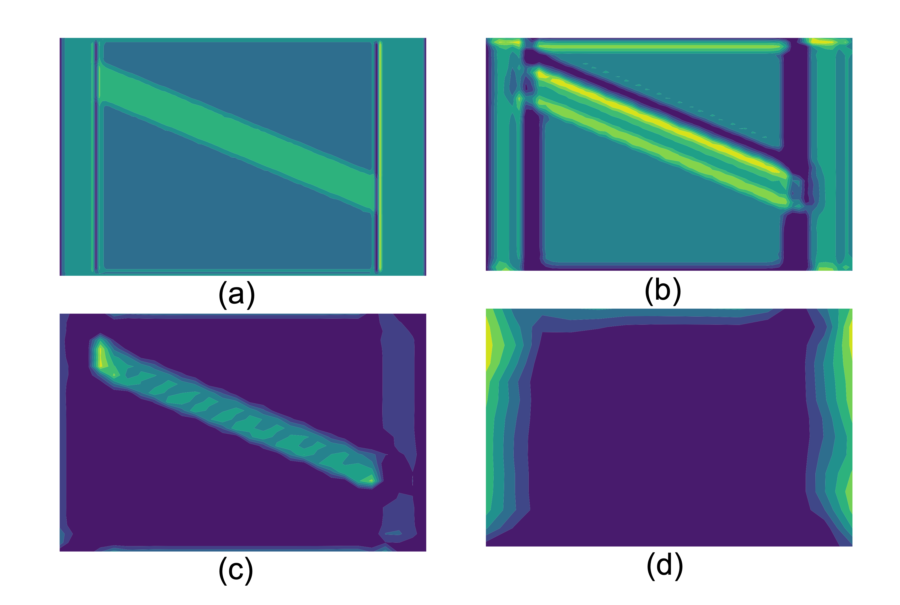
Figure 8: Intermediate steps output from the ResNetUNet decoding process.

The primary metrics to quantitatively evaluate the performance of the model are the MSE and MAE. The ground truth comes from the physics based simulation, and we are able to compare displacement values at each point in the image from prediction to simulation. This effectively quantifies the accuracy of the model. In order to quantitatively evaluate the performance of different models, we compare the training loss and validation loss for all three models in Fig. 9. The loss history illustrates that our model is tuned appropriately without overfitting or underfitting. The MSE and MAE errors are both collected and presented in the Tab. 3 as well.

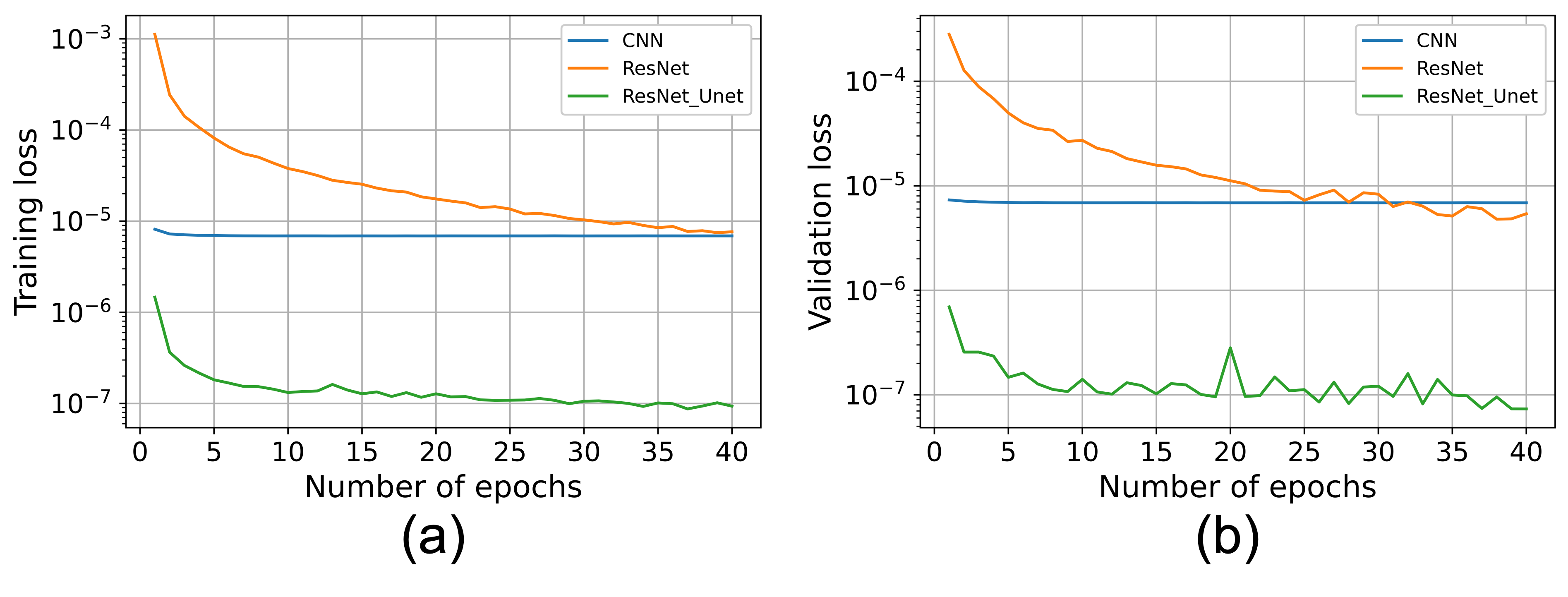
Figure 9: Training (a) and validation (b) loss change versus epoch number for all investigated models, including CNN, ResNet, and ResNetUNet.

Table 3: Comparison among CNN, ResNet and ResNetUNet using MSE and MAE loss values.

Model	Training loss		Validation loss
	MSE	MAE	MSE	MAE
CNN	6.89e-6	2.67e-3	6.88e-6	2.58e-3
ResNet	7.85e-6	2.22e-3	4.79e-6	2.00e-3
ResNetUNet	7.82e-8	1.90e-4	7.33e-8	2.00e-4

5.2 Transient mechanics model

It is essential to evaluate the transient mechanics model, because this is closer to the real world problems. The physics tells us the displacement could change over time when applied a constant load on a system having porous media with fluid inside it. Therefore, the problem changes from a static image to a time series video problem. We are motivated to use LSTM because it handles time series predictions well. And the transformer is getting more and more influential, so we decided to compare LSTM and transformer models.

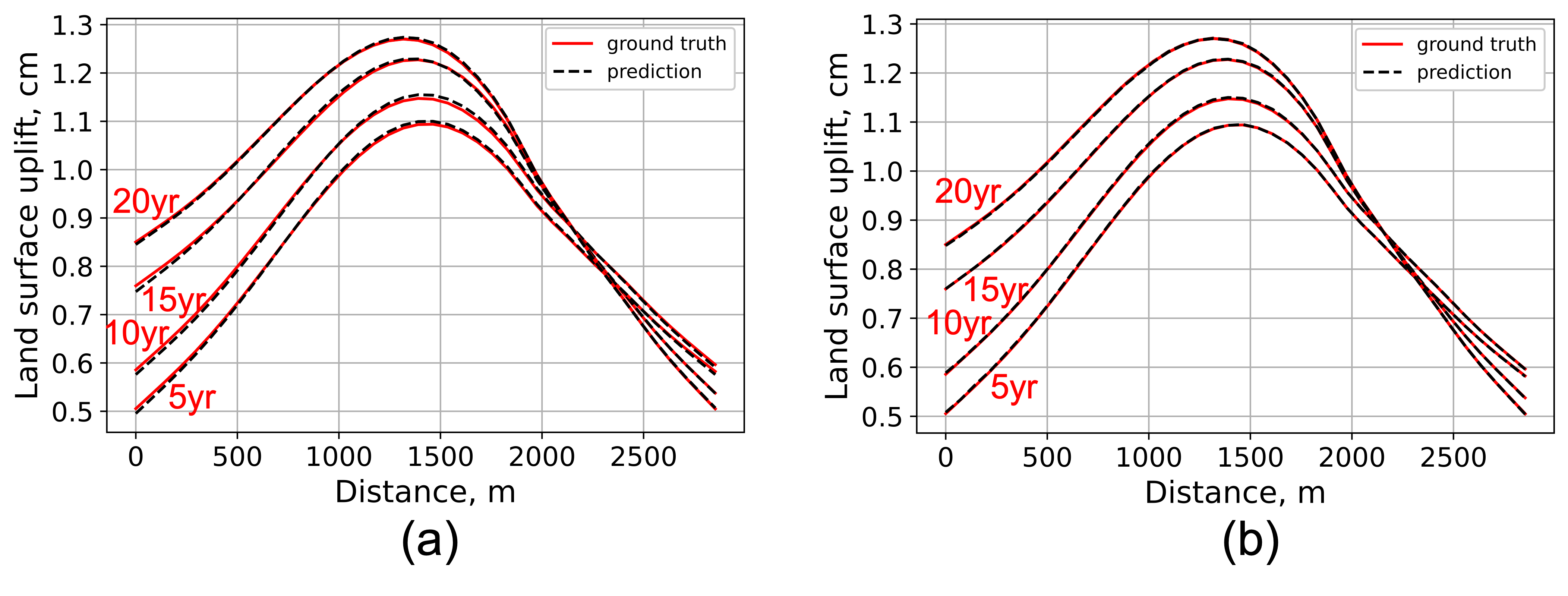
Figure 10: Predictions from (a) LSTM and (b) transformer for transient problem. We compare the surface uplift across the site at time of 5 years, 10 years, 15 years, and 20 years after the applied load in subsurface.

LSTM model has shown promising potential in time series prediction in various field sagheer2019time ; cao2019financial . However, the current data prediction mainly refers to the low-dimensional data, which is much lower than the case we deal with here, with dimension of 40. For the training of the LSTM model, we tune parameters including the number of LSTM cells, batch$\_$size, learning$\_$rate. Similarly, we use an Adam optimizer for the gradient descent. To avoid the overfitting and underfitting, we finally stack 4 LTSM cells, and we choose the batch$\_$size as 1024 to facilitate the execution in GPU. The learning$\_$rate is chosen as 0.001.

The validation loss history is shown in Fig. 11. The model is explored extensively, and we found that the LSTM prediction can fit the groundtruth with slight deviation. This is because we are predicting a value-based output with a high accuracy requirement, and the high dimension of the sequence requires an appropriate allocation of attention from the model. For example, the displacements in the middle of the domain have larger variation than the displacements at the corners, thus requiring more learning. The attention mechanism is not capable to deal with such a high dimensional data prediction task. This also inspires us to utilize a model with more attention, which gives rise to transformer.

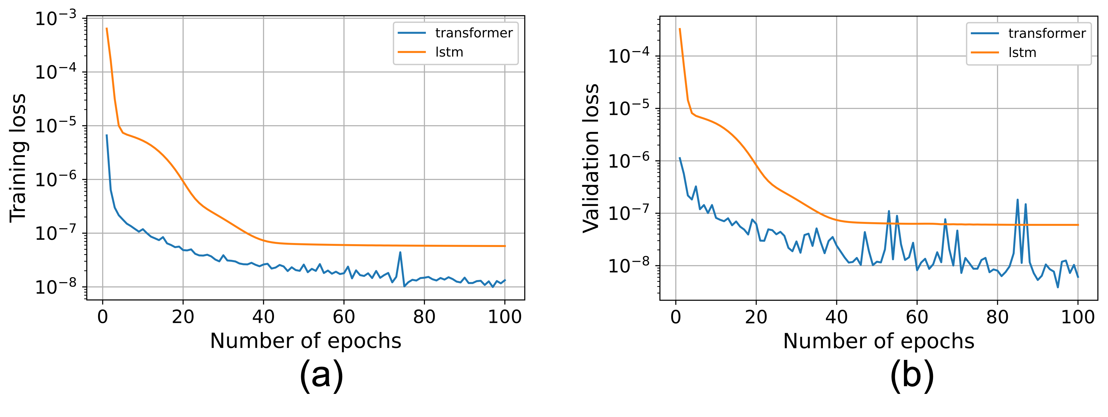
Figure 11: Comparison of model performance according to (a) training loss and (b) validation loss.

The transformer is well-tuned with the hyperparameters, such as learning$\_$rate and batch$\_$size, and the optimal value for the two parameters are the same as that of LSTM. Also, we set the dropout probability as 0.3 inside the transformer model. After running the same epochs of 100, transformer performs better than LSTM with lower loss and the prediction result also fits the groundtruth nearly perfectly. The loss history is illustrated in the Fig. 11 as well. To better quantify the LSTM and transformer model, we list the MSE and MAE in Tab. 4, which shows transformer performs better than LSTM in this case as well.

Table 4: Comparison among LSTM and transformer using MSE and MAE loss values.

Model	Training loss		Validation loss
	MSE	MAE	MSE	MAE
LSTM	6.89e-6	6.88e-6	6.00e-8	6.11e-6
Transformer	7.85e-6	2.81e-6	3.86e-9	1.50e-6

6 Conclusion and Future Work

This paper demonstrates a state-of-the-art approach to leverage computer vision intelligence for geomechanics computations. We generalize our problem for any input geometry images, and our trained models are no longer restricted to a specific case or field.

We observe the ResNetUNet model stands out compared to CNN and ResNet models for static displacement image predictions. The particular architecture of ResNetUNet ensures its excellent performance by passing the information from encoding to the decoding process. In comparison, CNN and ResNet models lose part of the information, although they successfully extract key features from input. The LSTM and transformer models work well for our transient part of work. We observe training a model for video problems requires larger RAM space due to more parameters involved. For all the models, we used both MSE and MAE as the way to quantify loss, and the comparison of training and validation loss indicates no underfitting or overfitting concerns. LSTM model shows less computational costs during the training, but we need to sacrifice prediction accuracy slightly. Both LSTM and transformer models indicate strong potential to solve the complex coupled solid mechanics and fluid flow problems, which is critical for carbon storage as one of the key components to mitigate global warming and protect our climate.

For future work, we will continue the path and generate more complicated input geometry images by using Generative Adversarial Networks (GAN) to test the performance of our models. The goal is to improve our model to be robust for land surface displacement predictions to inform decision making for carbon storage projects. In addition, we would like to launch our alpha version of web application for users to access our model, so that our work will contribute value to our society.

7 Supplementary Material

Get access to our source code in Github (Click Here).

For time series prediction, refer to the demo (Click here) to view the evolution of the displacement.

8 Acknowledgements

The authors thank Prof. Anthony Kovscek and Prof. Ronaldo Borja for valuable suggestions and advice in terms of carbon storage and rock mechanics. We acknowledge the insightful discussions with Ruohan Gao to improve our work on both image and video problems, and we also thank the support from Manasi, Sumith to formulate our work.

Appendix A. Physics formulation

For the static model, the mathematical formulation is: Formulating the problem set here further in a mathematical way, we solve a partial differential problem stated as: In terms of the domian $\Omega$, the boundary of the domain is denoted as $\Gamma=\Gamma_{u}\cup\Gamma_{t}$, where $\Gamma_{u}\cap\Gamma_{t}=\phi$, and the partial differential equations we are solving can be expressed as:

$$\nabla\cdot\boldsymbol{\sigma}+\rho\boldsymbol{g}=\boldsymbol{0},\ \boldsymbol{u}=\overline{\boldsymbol{u}}\ \text{on}\ \Gamma_{u},\ \boldsymbol{\sigma}\cdot\boldsymbol{n}=\overline{\boldsymbol{t}}\ \text{on}\ \Gamma_{t}$$ (6)

where $\boldsymbol{u}$ refers to displacement of the domain, $\boldsymbol{g}$ is the gravity acceleration, and the stress $\boldsymbol{\sigma}$ above is expressed as

$$\boldsymbol{\sigma}=\mathbb{C}^{e}:(\nabla\boldsymbol{u}+\boldsymbol{u}\nabla),$$ (7)

where $\mathbb{C}^{e}$ is the stiffness matrix.

For the transient model, the mathematical formulation is:

$$\nabla\cdot\boldsymbol{\sigma}+\rho\boldsymbol{g}=\boldsymbol{0},\ \boldsymbol{u}=\overline{\boldsymbol{u}}\ \text{on}\ \Gamma_{u},\ \boldsymbol{\sigma}\cdot\boldsymbol{n}=\overline{\boldsymbol{t}}\ \text{on}\ \Gamma_{t}$$ (8a)

$$\nabla\cdot\dot{\boldsymbol{u}}+\nabla\cdot{\boldsymbol{q}}=0,\ p=\overline{p}\ \text{on}\ \Gamma_{p},\ \overline{\boldsymbol{q}}=\overline{\boldsymbol{q}}\ \text{on}\ \Gamma_{q},$$ (8b)

where $\Gamma_{q}$ and $\Gamma_{p}$ are the essential and natural boundary for the pore pressure, and the stress $\boldsymbol{\sigma}$ is expressed as

$$\boldsymbol{\sigma}=\boldsymbol{\sigma}^{\prime}-p\mathbb{I},$$ (9)

$$\boldsymbol{\sigma}^{\prime}=\mathbb{C}^{e}:(\nabla\boldsymbol{u}+\boldsymbol{u}\nabla).$$

In addition to the symbols used in the static part, we have the pore pressure of fluid defined over the domain as $p$, and the fluid flux $\boldsymbol{q}=-\boldsymbol{\kappa}/\mu\nabla p$, which is Darcy’s law that associate the flux with the pore pressure by permeability $\boldsymbol{\kappa}$ and dynamic viscosity $\mu$.

References

- (1) A coupled reservoir simulation-geomechanical modelling study of the co2 injection-induced ground surface uplift observed at krechba, in salah. Energy Procedia, 37:3719–3726, 1 2013.
- (2) Martin Alnæs, Jan Blechta, Johan Hake, August Johansson, Benjamin Kehlet, Anders Logg, Chris Richardson, Johannes Ring, Marie E Rognes, and Garth N Wells. The fenics project version 1.5. Archive of Numerical Software, 3(100), 2015.
- (3) Klaus-Jürgen Bathe. Finite element method. Wiley encyclopedia of computer science and engineering, pages 1–12, 2007.
- (4) Yared W Bekele. Deep learning for one-dimensional consolidation. arXiv preprint arXiv:2004.11689, 2020.
- (5) Yoshua Bengio. Practical recommendations for gradient-based training of deep architectures. In Neural networks: Tricks of the trade, pages 437–478. Springer, 2012.
- (6) Stefan Braun. Lstm benchmarks for deep learning frameworks. arXiv preprint arXiv:1806.01818, 2018.
- (7) Jian Cao, Zhi Li, and Jian Li. Financial time series forecasting model based on ceemdan and lstm. Physica A: Statistical Mechanics and its Applications, 519:127–139, 2019.
- (8) Jason Charng, Di Xiao, Maryam Mehdizadeh, Mary S Attia, Sukanya Arunachalam, Tina M Lamey, Jennifer A Thompson, Terri L McLaren, John N De Roach, David A Mackey, et al. Deep learning segmentation of hyperautofluorescent fleck lesions in stargardt disease. Scientific Reports, 10(1):1–13, 2020.
- (9) Samantha J. Fuchs, D. Nicholas Espinoza, Christina L. Lopano, Ange Therese Akono, and Charles J. Werth. Geochemical and geomechanical alteration of siliciclastic reservoir rock by supercritical co2-saturated brine formed during geological carbon sequestration. International Journal of Greenhouse Gas Control, 88:251–260, 9 2019.
- (10) K Ho-Le. Finite element mesh generation methods: a review and classification. Computer-aided design, 20(1):27–38, 1988.
- (11) M Josh, L Esteban, C Delle Piane, J Sarout, DN Dewhurst, and MB Clennell. Laboratory characterisation of shale properties. Journal of Petroleum Science and Engineering, 88:107–124, 2012.
- (12) Nitish Shirish Keskar, Dheevatsa Mudigere, Jorge Nocedal, Mikhail Smelyanskiy, and Ping Tak Peter Tang. On large-batch training for deep learning: Generalization gap and sharp minima. arXiv preprint arXiv:1609.04836, 2016.
- (13) Diederik P Kingma and Jimmy Ba. Adam: A method for stochastic optimization. arXiv preprint arXiv:1412.6980, 2014.
- (14) Chao Li and Lyesse Laloui. Coupled multiphase thermo-hydro-mechanical analysis of supercritical co2 injection: Benchmark for the in salah surface uplift problem. International Journal of Greenhouse Gas Control, 51:394–408, 8 2016.
- (15) Qi Li, Guizhen Liu, Xuehao Liu, and Xiaochun Li. Application of a health, safety, and environmental screening and ranking framework to the shenhua ccs project. International Journal of Greenhouse Gas Control, 17:504–514, 2013.
- (16) Wei Liu, Sihan Chen, Longteng Guo, Xinxin Zhu, and Jing Liu. Cptr: Full transformer network for image captioning. arXiv preprint arXiv:2101.10804, 2021.
- (17) Xuhui Meng and George Em Karniadakis. A composite neural network that learns from multi-fidelity data: Application to function approximation and inverse pde problems. Journal of Computational Physics, 401:109020, 1 2020.
- (18) Zhenguo Nie, Haoliang Jiang, and Levent Burak Kara. Stress field prediction in cantilevered structures using convolutional neural networks. Journal of Computing and Information Science in Engineering, 20(1):011002, 2020.
- (19) Olaf Ronneberger, Philipp Fischer, and Thomas Brox. U-net: Convolutional networks for biomedical image segmentation. In International Conference on Medical image computing and computer-assisted intervention, pages 234–241. Springer, 2015.
- (20) Alaa Sagheer and Mostafa Kotb. Time series forecasting of petroleum production using deep lstm recurrent networks. Neurocomputing, 323:203–213, 2019.
- (21) Moses Soh. Learning cnn-lstm architectures for image caption generation. Dept. Comput. Sci., Stanford Univ., Stanford, CA, USA, Tech. Rep, 2016.
- (22) Jennie C Stephens. Growing interest in carbon capture and storage (ccs) for climate change mitigation. Sustainability: Science, Practice and Policy, 2(2):4–13, 2006.
- (23) M. Talebian, R. Al-Khoury, and L. J. Sluys. A computational model for coupled multiphysics processes of co2 sequestration in fractured porous media. Advances in Water Resources, 59:238–255, 9 2013.
- (24) Ying Hua Tan and Chee Seng Chan. Phrase-based image caption generator with hierarchical lstm network. Neurocomputing, 333:86–100, 2019.
- (25) Meng Tang, Xin Ju, and Louis J. Durlofsky. Deep-learning-based coupled flow-geomechanics surrogate model for co2 sequestration. 5 2021.
- (26) Meng Tang, Yimin Liu, and Louis J. Durlofsky. A deep-learning-based surrogate model for data assimilation in dynamic subsurface flow problems. Journal of Computational Physics, 413:109456, 7 2020.
- (27) Ashish Vaswani, Noam Shazeer, Niki Parmar, Jakob Uszkoreit, Llion Jones, Aidan N Gomez, Łukasz Kaiser, and Illia Polosukhin. Attention is all you need. Advances in neural information processing systems, 30, 2017.
- (28) Ashish Vaswani, Noam Shazeer, Niki Parmar, Jakob Uszkoreit, Llion Jones, Aidan N Gomez, Ł ukasz Kaiser, and Illia Polosukhin. Attention is all you need. In I. Guyon, U. Von Luxburg, S. Bengio, H. Wallach, R. Fergus, S. Vishwanathan, and R. Garnett, editors, Advances in Neural Information Processing Systems, volume 30. Curran Associates, Inc., 2017.
- (29) Victor Vilarrasa, Diogo Bolster, Sebastia Olivella, and Jesus Carrera. Coupled hydromechanical modeling of co2 sequestration in deep saline aquifers. International Journal of Greenhouse Gas Control, 4:910–919, 12 2010.
- (30) Gege Wen, Meng Tang, and Sally M. Benson. Towards a predictor for co2 plume migration using deep neural networks. International Journal of Greenhouse Gas Control, 105:103223, 2 2021.
- (31) Kailai Xu and Eric Darve. Physics constrained learning for data-driven inverse modeling from sparse observations. 2 2020.
- (32) Albert Zeyer, Parnia Bahar, Kazuki Irie, Ralf Schlüter, and Hermann Ney. A comparison of transformer and lstm encoder decoder models for asr. In 2019 IEEE Automatic Speech Recognition and Understanding Workshop (ASRU), pages 8–15. IEEE, 2019.
- (33) Qiang Zheng, Lingzao Zeng, and George Em Karniadakis. Physics-informed semantic inpainting: Application to geostatistical modeling. Journal of Computational Physics, 419:109676, 10 2020.
- (34) Yongjin Zhou, Weijian Huang, Pei Dong, Yong Xia, and Shanshan Wang. D-unet: a dimension-fusion u shape network for chronic stroke lesion segmentation. IEEE/ACM transactions on computational biology and bioinformatics, 18(3):940–950, 2019.