Economic Capacity Withholding Bounds of Competitive Energy Storage Bidders

Abstract

Problem definition: Economic withholding in electricity markets refers to generators bidding higher than their true marginal fuel cost, and is a typical approach to exercising market power. However, existing market designs require storage to design bids strategically based on their own future price predictions, motivating storage to conduct economic withholding without assuming market power. As energy storage takes up more significant roles in wholesale electricity markets, understanding its motivations for economic withholding and the consequent effects on social welfare becomes increasingly vital. Methodology/results: This paper derives a theoretical framework to study the economic capacity withholding behavior of storage participating in competitive electricity markets and validate our results in simulations based on the ISO New England system. We demonstrate that storage bids can reach unbounded high levels under conditions where future price predictions show bounded expectations but unbounded deviations. Conversely, in scenarios with peak price limitations, we show the upper bounds of storage bids are grounded in bounded price expectations. Most importantly, we show that storage capacity withholding can potentially lower the overall system cost when price models account for system uncertainties. Managerial implications: Our paper reveals energy storage is not a market manipulator but an honest player contributing to the social welfare. It helps electricity market researchers and operators better understand the economic withholding behavior of storage and reform market policies to maximize storage contributing to a cost-efficient decolonization.

1 Introduction

Energy storage participants are becoming key players in wholesale electricity markets. In the California Independent System Operator (CAISO), the capacity of utility-scale battery energy storage has already exceeded 5 GW and is projected to surpass 10 GW in the upcoming five years [1]. Following California’s lead, Texas has emerged as the second-largest market in storage capacity terms [2]. Consequently, the role of storage in the market has naturally transitioned from ancillary service markets to price arbitrage in wholesale markets, reflecting the significant capacity influx [3]. It’s now crucial to comprehend the factors influencing energy storage market participation. Such understanding is essential for formulating regulatory policies, addressing market power concerns, and crafting effective price signals [4].

Energy storage participants employ bidding strategies that fundamentally differ from those of conventional generators. While existing competitive electricity market designs incentivize conventional generators to base their bids on fuel costs [5], energy storage participants must integrate future opportunity values into their bid designs [6]. This is primarily because their immediate operations are influenced by anticipated price outcomes, especially in real-time markets that only clear for the imminent hour [7, 8]. Consequently, storage entities must operate with strategic foresight [9] in the present market framework, and exercise economic capacity withholding such that their bids are higher than their physical production costs. This perspective is also reflected in CAISO’s recent market power mitigation manual, which acknowledges that storage bids should account for opportunity costs and should “include the highest (predicted) price, corresponding to the storage duration of the resource" [10].

Due to the significant volatility inherent in real-time power system operations, it is impractical for storage participants to expect designing bids using accurate price predictions [11]. A more pragmatic approach to increase profit potential is thus to incorporate uncertainty price models into bid design [12]. Hence, a pivotal consideration emerges with the growth of storage market share: How would uncertainty models employed in storage’s bidding strategy affect their profit and the operating cost of the entire system? A good understanding of this problem can provide insights into future market mechanisms and regulatory framework designs.

This paper studies the economic capacity withholding behavior of storage participating in competitive electricity markets. We assume the storage has no intention of exercising market power. Hence, the withholding amount is solely dictated by the price prediction and the associated uncertainties. Our study offers the following key contributions:

1. We introduce a theoretical framework to understand the economic capacity withholding motivations in storage bid design and the associated uncertainty models, characterized by stochastic dynamic programming, in competitive electricity markets.

2. We prove that if the electricity price is unbounded, then economic withholding of storage, i.e., the bid values, can become arbitrarily high based on the uncertainty model of the price while having bounded price expectations.

3. We derive the storage economic withholding bounds in cases when the electricity market prices are bounded and discuss variations of this model to price distribution functions, such as the dependence on price spike occurrences.

4. We show that storage units when utilizing uncertainty models for market bid formulation, can potentially lower the overall system cost when the system encounters a suitable level of uncertainty.

5. We validate our result using an agent-based market simulation with Monte-Carlo scenarios based on the ISO New England system.

The remainder of the paper is organized as follows. Section 2 reviews related literature. Section 3 formulates the market clearing and storage bidding models and clarifies the definition of economic capacity withholding. Section 4 presents our theoretical results of the storage withholding bounds and welfare-aligned withholding. Section 5 shows the simulation results of proposed theorems and extend the proposed theorem to practical market settings, and Section 6 concludes this paper. Detailed proofs are provided in Appendix.

2 Backgrounds

2.1 Uncertainty management in power systems

Employment of uncertainty models in power systems operations is increasingly critical due to rising forecast errors contributed by progressive deployments of intermittent renewables [13]. The operational constraints, such as generator start-up/shut-down requirements, ramp speeds, and storage limits, limit the flexibility of most generators to adapt swiftly to immediate set-point changes [5]. Consequently, the planning of operations must anticipate and accommodate these limitations with respect to uncertainty factors in power systems.

Over the past decade, researchers have proposed various approaches to address increasing uncertainties in power system scheduling utilizing methods such as stochastic optimization [14, 15], robust optimization [16, 17], and other risk-aware methods [18, 19, 20]. While methodologically diverse, a common assumption in these frameworks is the central role of the power system operator in uncertainty management. This responsibility entails the development of stochastic models for renewable energy supply and demand, establishing risk preferences for dispatch, and integrating additional objectives and constraints into the market-clearing model.

However, solely relying on a centralized approach may not be practical. Firstly, the complexity of many uncertainty models can substantially increase the computational burden of power system optimizations, hindering their implementation over real-world systems [21]. Secondly, in deregulated power systems, where supply and demand are balanced through market clearing, the operator must maintain a neutral stance. Centralizing uncertainty management will inevitably cause market prices to be affected by the uncertainty preference set by the power system operators and may not capitalize on the advantages of distributed decision-making and risk assessment. It is thus increasingly important to analyze uncertainties in electricity markets as strategic interactions between market participants hedge against risks [22].

2.2 Economic capacity withholding of storage

Capacity withholding is a strategy where generators conserve a portion of their capacity inaccessible to market clearings. This can manifest in two ways: physical withholding, where a generator offers less capacity than available; and economic withholding, where a generator sets its offer prices above its actual marginal cost, leading to reduced capacity clearance at a specific market clearing price. A direct consequence of capacity withholding is steeper supply curves, resulting in higher market prices and, thus, higher profit of generation units despite less cleared quantity. Capacity withholding is a common practice to exercise market power [5].

While identifying physical capacity withholding is straightforward based on the rated unit capacity, economic capacity withholding is significantly more sophisticated regarding energy storage. Harvey and Hogan [6] have acknowledged energy-limited resources (which would include today’s energy storage) may withhold capacity in certain hours due to expectations of higher future prices, i.e., opportunity cost, and such behaviors should be distinguished from the exercise of market power in that “efficient pricing would fully utilize the energy of the unit in the highest price hours over the period of the limitation”. Yet, they remarked that the lack of perfect foresight, hence uncertainty or imperfect judgment, “could have a larger impact on reducing supply than the exercise of market power”. They also made an important statement that economic withholding of energy-limited resources is “necessary to the efficient and reliable operation of the electric grid”.

It is worth noting that Harvey and Hogan’s 2001 study primarily referenced liquefied natural gas (LNG) and pumped hydro resources. These resources held a relatively marginal presence in the electricity markets of that era, and their market impact was limited. Moreover, their operational characteristics differ considerably from today’s battery energy storage. For instance, LNG storage incurs consistent fuel costs, while pumped hydro operations must account for environmental and water supply constraints [23]. Hence, given the associated modeling complexity and the limited impact in practice, the paper concluded that perhaps the most realistic option is to “exempt them (energy limited resources) from the no economic or physical withholding standard”.

With the notable rise of battery energy storage in recent years, many studies have delved into the market behavior of these storage resources. A considerable body of research underscores how integrating uncertainty price models into storage bid designs can improve market profits, especially in the face of market and system fluctuations [12, 24, 25, 26, 27, 28, 29]. Storage can also seek to exercise market power like conventional generators to drive up prices and gain more profits [30, 31]. Apparently, storage can combine uncertainties and market powers to maximize their market return using more sophisticated bidding models [32]. Recent studies have also investigated storage bidding behaviors and their consequent market ramifications from the system’s perspective [33, 34]. However, a comprehensive exploration into the specific capacity withholding practices of storage and its systemic implications remains noticeably absent from current literature.

3 Formulation and Preliminaries

We first present the market clearing model considered in this study, followed by the storage bidding model considering uncertain future price predictions. We also present some results that are prerequisites to our main results, including storage bid design and bid incorporation into the market clearing model.

3.1 Market clearing model

We consider a typical two-stage energy market consisting of day-ahead markets (DAM) and real-time markets (RTM). The DAM performs unit commitment over the next 24 hours, followed by sequential real-time dispatches. Our study focuses on energy storage participation in RTM as shown in Figure 1. As a participant, storage submits bids to the system operator in a manner akin to a conventional generator. After receiving bids from storage and generator participants, the system operator clears the RTM, issuing both dispatch commands and release clearing prices.

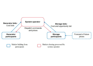
Figure 1: Storage participation in RTM.

To focus on the relationship between storage bidding models and system uncertainties, we consider a single-bus and single-storage system in which the storage acts as a price taker but takes price uncertainties into the bid design. For a time step $t\in\mathcal{T}$, the RTM clearing is thus formulated as

$$\min_{g_{t},\leavevmode\nobreak\ p_{t},\leavevmode\nobreak\ b_{t}}\;G_{t}(g_{t})+O_{t}(p_{t})-B_{t}(b_{t}),$$ (1a)

where $$\mathcal{T}=\{1,2,3,...,T\} T g_{t} G_{t} p_{t} b_{t} t p_{t} b_{t} O_{t} B_{t}$$ indicates the set of periods, in which 1 and indicates the first and the last period of an operating day, respectively. is the aggregated power generation of conventional generators, and is the aggregated generation cost function. and are the energy discharged/charged into the storage over time period , which are also referred to as the power rating in some literature. Note that we have normalized the time period duration into and , thereby eliminating the need for a duration coefficient to maintain clarity in our presentation. and are the supply (discharge) offer cost function and the demand (charge) bidding function of storage, respectively.

The RTM includes the power balance constraint, as shown in equation (1b). The associated dual variable, $\lambda_{t}$, represents the market clearing price

$$g_{t}+p_{t}-b_{t}=D_{t}-w_{t},$$ (1b)

in which $w_{t}$ is the renewable generation and $D_{t}$ is the demand. Note that $D_{t}-w_{t}$ is the net demand and is also the source of uncertainty in real-time power system operations.

The RTM models the storage unit constraints. Equation (1c) models the discharge energy limit over period $t$, which is the lesser of the limit $P$ and the energy left in the storage $e_{t-1}$ modulated by the discharge efficiency $\eta$; Similarly, equation (1d) models the charging energy limit, which is the lesser of the limit $P$ and the charging headroom given full storage capacity $E$

$$0\leq p_{t}\leq\min\{P,e_{t-1}\eta\},$$ (1c)

$$0\leq b_{t}\leq\min\{P,\frac{E-e_{t-1}}{\eta}\}.$$ (1d)

The market clearing is also subject to generator unit constraints, which are omitted in the main text for simplicity. For the full market clearing model formulation, including DAM and RTM that we used in our simulation, please refer to Appendix 6.1.

3.2 Storage bidding model

In this subsection, we elaborate on the bidding model of the storage participant, who acts as a price taker but takes price uncertainty into bidding design. As shown in Figure 1, a storage participant acts like a generator, but it takes opportunity values, together with physical costs, into bid design considering storage’s nature as a limited energy sources. Storage’s physical cost is associated with its physical parameters like efficiency and marginal discharging costs, while its opportunity cost is dependent on it forecast of future prices. Specifically, we assume the storage models the future real-time price as a time-varying stage-wise independent process, $\hat{\lambda}_{t}$.

Remark 1.

Day-ahead to real-time price convergence. The expectation of real-time prices is approximately the day-ahead market clearing price of the same time period [35]. This convergence is facilitated by two factors. First, most suppliers and demands in electricity markets are settled in day-ahead markets, while real-time markets primarily settle the deviations to day-ahead settlements. Hence, real-time prices should be distributed around the day-ahead price. Second, virtual bids, in which market speculators can arbitrage between day-ahead and real-time markets, create incentives for participants to converge persistent price gaps between day-ahead to real-time.

Thus, all RTM price models explored in this paper have fixed expectations in all bounded and unbounded cases, i.e., $\mu_{t}$ is fixed for $\forall t\in\mathcal{T}$.

Hence, the storage arbitrage problem can be formulated as stochastic dynamic programming (SDP) as

$$Q_{t-1}(e_{t-1}|\hat{\lambda}_{t}) :=\max_{p_{t},b_{t}}\hat{\lambda}_{t}(p_{t}-b_{t})-cp_{t}+V_{t}(e_{t})$$ (2a)

$$V_{t-1}(e_{t-1}) :=\mathbb{E}_{\hat{\lambda}_{t}}\Big{[}Q_{t-1}(e_{t-1}|\hat{\lambda}_{t})\Big{]}$$ (2b)

subjects to

$$0 \leq p_{t}\leq P\mathbf{1}_{[\hat{\lambda}_{t}\leq 0]}$$ (2c)

$$0 \leq b_{t}\leq P$$ (2d)

$$e_{t}-e_{t-1} =-p_{t}/\eta+b_{t}\eta$$ (2e)

$$0 \leq e_{t}\leq E$$ (2f)

where $c$ is the physical discharge cost, and $V_{t}$ is the value-to-go function recursively defined as the optimized profit expectation in the future. (2c) and (2d) are the discharging and charging energy constraints, respectively. Note in (2c) that the indicator function on the upper energy limit enforces the discharge energy to be zero if the price is smaller than zero, hence preventing the battery from discharging at negative prices. This condition is sufficient to prevent simultaneous charge and discharge and will be an important property to utilize in our later results. (2e) is the state-of-charge (SoC) efficiency constraint, and (2f) is the energy capacity constraint. Also note that (2c)–(2f) are equivalent to (1c) and (1d), which enforces power and energy rating subjecting to efficiencies. The difference is that we consider a RTM clearing model so there is no need for the system operator to model SoC constraints explicitly and can integrate energy limits into the power rating, while the storage bidding model solves a multi-period optimization.

Remark 2.

Finite horizon and end value function. Given the limited time horizon market information available to storage operators, we consider the SDP bidding problem to have a finite horizon (such as end of the day) with a terminal value function $V_{T}(e_{T})$ representing the final value of energy stored. Note that $V_{T}(e_{T})$ can be simply set to zero to show no final energy value.

Proposition 1.

Storage bid curve. Given the calculated storage value functions, we generate the storage offer curve and bid curve based on the subderivatives of the cost functions, i.e., the marginal cost curve

$${O}_{t}(p_{t}) =\Big{[}c+\frac{1}{\eta}v_{t}(e_{t})\Big{]}^{+}=\Big{[}c+\frac{1}{\eta}v_{t}(e_{t-1}-p_{t}/\eta)\Big{]}^{+}$$ (3a)

$${B}_{t}(b_{t}) =\eta v_{t}(e_{t})=\eta v_{t}(e_{t-1}+b_{t}\eta)$$ (3b)

where $[x]^{+}=\max\{0,x\}$ is used to reflect constraint (2c) that no discharge power would be cleared during negative prices.

Note that within the RTM framework, a storage participant is expected to bid as a generator and a load. Consequently, the storage bids, represented by the functions $O_{t}(p_{t})$ for discharging and $B_{t}(b_{t})$ for charging, are formulated based on the amount of energy discharged and charged, respectively, instead of focusing on the SoC $e_{t}$. The marginal value function $v_{t}(e_{t})$ is defined as

$$v_{t}(e_{t})=\max\leavevmode\nobreak\ \partial V_{t}(e_{t})$$ (4)

where $\partial V_{t}(e_{t})=\cap_{z\in\textbf{dom}V_{t}}\{g|{V_{t}}(z)\geq{V_{t}}(e_{t})+g^{T}(z-e_{t})\}$ is the subderivative at $e_{t}$. Equation (4) presents $v_{t}(e_{t})$ is the partial derivative of $V_{t}$ when $V_{t}$ is differentialable at $e_{t}$, and is the maximal subgradient value at the corner point $e_{t}$ when $V_{t}$ is not differentialable.

The bidding curve results show that the bid-offer curves consist of the physical discharge cost $c$ and the opportunity value component based on the marginal value function $v_{t}$. Note that in cases when markets require price-quantity segment offer curves, the bid function can be discretized based on power segments.

The proof of this proposition is trivial by taking the subderivative of the storage cost, represented as the second and third term in (2a), with respect to the charge or discharge energy. We utilize (2e) to calculate the partial subderivative of $e_{t}$ to $p_{t}$ and $b_{t}$, then apply the partial derivative chain rule. Finally, we utilize (2e) again to substitute $e_{t}$ with $e_{t-1}$ and discharge/charge energy since $e_{t-1}$ is a known state to the storage operator and serves as input to the bid curve. The range of the bid curves follows the feasible range of discharge and charge energy as defined in (1c) and (1d), respectively.

Remark 3.

Storage opportunity bids. Different from generators that bid based on physical costs, the storage design bids based on opportunity costs. For example, as shown in equation (2b), storage value $V_{t-1}$ is dependent on its price prediction of the next period $\hat{\lambda}_{t}$ as well as the value function $V_{t}$ at period $t$. Similarly, $V_{t}$ is dependent on the price prediction and its value function of period $t+1$. Recursively, we know storage value at period $V_{t-1}$ is dependent over price forecasts of periods $t,t+1,t+2,...,T$. In practice, storage opportunity bids have been acknowledged by system operators like California ISO [10].

We now show the value function $V_{t}(e_{t})$ will always be concave for any price distributions given a concave end value function $V_{T}(e_{T})$, and the storage bids will always be convex.

Proposition 2.

Concave value function. Given a concave end value function $V_{T}(e_{T})$, then $V_{t}(e_{t})$ is concave for all $t\in\mathcal{T}^{{}^{\prime}}=\{1,2,3,...,T-1\}$ and for all price distribution functions $\hat{\lambda}_{t}\in\hat{\lambda}(\bm{\mu},\bm{\sigma}^{2})$.

Proposition 2 states that the value of energy stored is a concave function that follows the law of diminishing returns, hence, the more energy stored, the less marginally valuable they are. We defer the complete proof to Appendix 6.2.

Corollary 1.

Convex storage bids. Given a concave end value function $V_{T}(e_{T})$, ${O}_{t}(p_{t})$ monotonically increases with $p_{t}$, ${B}_{t}(b_{t})$ monotonically decreases with $b_{t}$, hence the market clearing model in (2) is always convex.

This corollary is trivial to show based on Proposition 2, which proves $V_{t}(e_{t})$ is always concave. Then $v_{t}(e_{t})$ is a monotonically decreasing function. Then we can finish the proofs according to (3).

At this point, we have shown if the storage model is linear, then all its bid curves will fit the convex market clearing model under stochastic bid design objectives under any assumed price distributions.

3.3 Economic capacity withholding storage bids

We now formally define non-withholding capacity bids for storage and state our definition of economic withholding. We are building up our framework on the perspective of Harvey and Hogan [6] that states the economic capacity withholding intentions of energy-limited resources can only be identified after-the-fact but must also account for the imperfect foresight. First, we introduce the following proposition to show that non-withholding bids of a linear storage model should always be constant bids if 1) it does not assume market power, 2) it assumes deterministic future price forecast, and 3) the final SoC value is also a linear function.

Proposition 3.

Deterministic storage bids. If $\sigma_{t}^{2}=0$ in equation (2), then storage bid curves will be constant if $V_{T}(e_{T})$ is a linear function. Hence, $O_{t}(p_{t})$ and $B_{t}(b_{t})$ as in (3) are linear.

Proof.

The proof of this proposition is based on using Simplex algorithm [36], which states the optimal solution of linear programming must be on a polyhedral vertex. Note that if there is no uncertainty, then (2) becomes equivalent to the following linear programming formulation with a strict linear objective function (not piece-wise linear)

$$\max_{p_{t},b_{t}}\sum_{t=1}^{T}\hat{\lambda}_{t}(p_{t}-b_{t})-cp_{t}+V_{T}(e_{T})$$ (5)

subjects to (2c)–(2f) for all $t\in\mathcal{T}.$ Then $p_{t}$ and $b_{t}$ must be bonded by one of the constraints, including the upper/lower energy limits and the SoC limits factoring in efficiency. Thus, for all price predictions $\hat{\lambda}_{t}$ and beginning SoC $e_{t-1}$ for all time period $t\in\mathcal{T}$, the storage dispatch solution will be either charging at $b_{t}=\min\{P,(E-e_{t-1})/\eta\}$, idle ($p_{t}=0$, $b_{t}=0$), or discharging at $p_{t}=\min\{P,e_{t-1}\eta\}$. Then there is no slope between charge or discharge energy to the price $\hat{\lambda}_{t}$. In other words, if we fix all other prices and only perpetuate the price realization of any particular time interval, it will cause the storage at that time period to switch between fully charging, idle, and fully discharging. This is equivalent to a constant supply or bid curve, as the storage will offer full capacity if the price is above or below a certain threshold. Hence, we finished the proof. ∎

4 Main Results

Our theoretical results solely focus on supply capacity withholdings since in electricity markets, capacity withholdings typically refer to supply offers, and there are fewer concerns regarding demand withholdings. Nevertheless, the theoretical frameworks for analyzing supply and demand withholding of storage are symmetrical with opposite directions regarding the propagation of value functions with respect of SoC. Hence, in our results, we will not discuss demand withholdings.

We first demonstrate the concavity of storage value functions across all potential price distributions – a crucial property referenced in subsequent findings. Then we show if the price maintains a consistent expectation but has an unbounded distribution, the corresponding storage bid also remains unbounded. Conversely, with a bounded price distribution defined by upper and lower price thresholds, the storage bid will also bounded, and we will detail its upper bound formulation. We’ll further explore various corollaries tied to different price distribution scenarios. Lastly, we’ll comment on the interplay between storage bidding uncertainty models and overall market welfare.

4.1 Unbounded economic capacity withholding

Traditional market price analysis focuses solely on the price expectations (i.e., average price values), but there are fewer concerns over the price deviations, hence the volatility. Our results state that even with a given price expectation, the storage economic capacity withholding, i.e., the bid values, can be arbitrarily high based on the price standard deviation when assuming the price follows a Gaussian distribution.

Theorem 1.

Unbounded withholding with Gaussian distributions. Assume the storage owner anticipates future prices following Gaussian distributions with fixed expectations but unbounded variance. Given arbitrary time interval $t\in\mathcal{T}^{{}^{\prime}}$, for a given price expectation over the next time period, $\mu_{t+1}$, for an arbitrary bid value $\theta\geq 0$, there exists a standard deviation $\sigma_{t+1}\geq\underline{\sigma}$ such that

$$v_{t}(0)\geq\theta.\leavevmode\nobreak\$$ (6)

where constant $\underline{\sigma}$ represents the lower bound essential for always ensuring the validity of inequality (6) at all times.

Theorem 1 asserts that unbounded price distributions can render storage economic capacity withholding in boundless. This theorem goes beyond the conventional analysis of market prices, highlighting a crucial nuance: Even when storage anticipates a fixed price expectation for the next period, the existence of an unbounded deviation can result in an unbounded marginal value function for storage. Consequently, this leads to unbounded withholding in RTM.

The proof of Theorem 1 is first based on the following Lemma.

Lemma 1.

Given $v_{T}(e_{T})\geq 0,\leavevmode\nobreak\ \forall e_{T}\in[0,\leavevmode\nobreak\ E]$ and the storage’s duration $E\geq 2P/\eta$, then $v_{t}(P\eta)\geq 0,\forall t\in\mathcal{T}^{{}^{\prime}}$.

Lemma 1 asserts that initiating storage charging for a single time period from zero SoC will not immediately result in the marginal value function $v_{t}(e_{t})$ dropping below zero for all $t\in\mathcal{T}$. The idea to prove Lemma 1 is trivial. Considering $q_{t}(0|\hat{\lambda}_{t+1})$ monotonically increases with $\hat{\lambda}_{t+1}$, we can find the lower bound of $q_{t}(0|\hat{\lambda}_{t+1})$ and its expectation, $v_{t}(0)$. Then we can prove the lower bound larger than zero. Detailed proof can be found in Appendix 6.6.

Following up on Lemma 1, the proof to Theorem 1 is sketched as follows. First, we must find the exact expression of $\underline{\sigma}$ and prove the unbounded marginal value function. The approach to proving this theorem hinges on establishing the monotonic increase of $v_{t}(0)$ concerning the deviation $\sigma_{t+1}$. To accomplish this, we initially identify the lower bound of $v_{t}(0)$ based on the conclusion of Lemma 1. We subsequently demonstrate the monotonic increase of this lower bound with respect to the deviation $\sigma_{t+1}$, thereby providing us with the crucial value of $\underline{\sigma}$. For detailed proofs of Theorem 1, please refer to the Appendix 6.3.

Corollary 2.

Unbounded withholding for distributions of generalized types with at zero SoC. Given arbitrary time interval $t\in\mathcal{T}^{{}^{\prime}}$ and a concave value function $V_{t+1}$, for an arbitrary value $\theta\geq 0$ and an arbitrary price expectation $u_{t+1}$, there exists a distributions $\hat{\lambda}_{t+1}$ such that

$$v_{t}(0)\geq\theta\text{ and }\mathbb{E}[\hat{\lambda}_{t+1}]=\mu_{t+1},$$ (7)

which indicates storage economic withholding $O_{t}$ is unbounded.

Corollary 2 extends the insights of Theorem 1 to encompass various distribution types, offering a more comprehensive understanding: In essence, the corollary suggests that storage dynamically updates its opportunity value by effectively aligning it with the latest peak price at its minimum SoC. This implies that the final segment of retained energy is strategically earmarked for sale during intervals with the most favorable projected future prices.

Subsequently, the main proof of this corollary articulates that once the storage revises its opportunity value linked to a SoC level to a more elevated price, the prior opportunity value is then transferred to the succeeding elevated SoC levels. This conveys that if storage perceives a unit of energy (SoC) can be traded at a price higher than previously estimated, it logically follows that the subsequent storage unit can be sold at the formerly estimated price. Detailed proofs of Corollary 2, please refer to the Appendix 6.4.

Corollary 3.

Unbounded withholding with extended bidding intervals. Given arbitrary time interval $\tau\in\mathcal{T}$ and starting SoC $e_{\tau-1}\in[0,E]$, for an arbitrary bid value $\theta\geq 0$ and an arbitrary trajectory of future price expectations $u_{t}$, there exists a set of future price distributions $\hat{\lambda}_{t}$ such that for any $p\in[0,\min\{P,e_{\tau-1}\eta\}]$

$$O_{\tau}(p_{\tau})\geq\theta\text{ and }\mathbb{E}[\hat{\lambda}_{t}]=\mu_{t}|t\in\{\tau,\dotsc,T\},$$ (8)

if $T-t\geq(e_{\tau-1}\eta-p_{\tau})/P$.

Corollary 3 shows that given a set of price predictions with fixed price expectations, storage bids can skyrocket to any value within a time interval, as long as the remaining time intervals in the bidding problem are sufficient for the storage to discharge completely. The flexibility for the storage bidder to extend the bidding horizon implies that the storage can strategically withhold any economic capacity based on assumed price distributions without altering the overall expectation. The proof of the Corollary 3 is based on the proofs of Corollary 2, which will be provided in Appendix 6.5.

4.2 Bounded economic capacity withholding

In practice, the system operator of electricity markets usually imposes price floors and ceilings, hence the distribution of the price is bounded. In this section, we present results about the storage economic withholding bid bounds based on bounded prices with fixed or bounded expectations.

Theorem 2.

Bounded withholding with bounded prices. Assume the storage has a linear final value function $V_{T}(e)=\sigma_{t}\cdot e$ with $\sigma_{t}\geq\Big{[}(\underline{\lambda}-c)\eta\Big{]}^{+}$, and market prices have an upper bound $\overline{\lambda}$ and a lower bound $\underline{\lambda}$. Then, the storage bidding price has the following upper bound given $t\in\mathcal{T}^{{}^{\prime}}$:

$$O_{t}(p_{t}) \leq c+\Big{(}\overline{\lambda}-c\Big{)}\sum_{i=t+1}^{T}\alpha_{i}\prod_{\tau=t+1}^{i-1}\beta_{\tau}+\prod_{\tau=t}^{T}\beta_{\tau}\frac{\sigma_{t}}{\eta}$$ (9a)

for all possible price distributions satisfying

$$\mathbb{E}(\hat{\lambda}_{t+1})=\mu_{t+1}\text{ and }\underline{\lambda}\leq\hat{\lambda}_{t+1}\leq\overline{\lambda}$$ (9b)

where $$\alpha_{t}=({\mu_{t}-\underline{\lambda}})/({\overline{\lambda}-\underline{\lambda}}) \beta_{t}=1-\alpha_{t} x_{1}\geq x_{2} \prod_{x_{1}}^{x_{2}}$$ and . Note that when , = 1.

Note the assumption on the final SoC value simply indicates the storage believes it can sell all energy stored at the end of the market period at the minimum market price $\underline{\lambda}$ in the future while also ensuring no discharge at negative prices as in (2c). The idea of proving Theorem 2 is that given the price bounds, then $v_{t}(0)$ is always maximized if the price is distributed at the maximum and minimum values, hence $\alpha_{t}$ is the occurrence of $\overline{\lambda}$ during interval $t$, while $\beta_{t}$ then is the occurrence of $\underline{\lambda}$ while ensuring the price expectation is $\mu_{t+1}$. Detailed proofs are given in Appendix 6.7.

The time-varying distribution of the price make Theorem 2 unapparent to observe, we now introduce the following corollary which assumes an upper bound of the price expectations.

Corollary 4.

Bounded withholding with bounded expectations. Following same assumptions in Theorem 2, now adding that all price expectations have an upper bound $\mu_{t}\leq\overline{\mu}$. All assume there is a interval-based discount ratio $\rho\in(0,1]$, then the upper storage bid bound becomes

$$O_{t}(p_{t}) \leq c+\frac{\alpha}{1-\rho\beta}(1-\beta^{T-1})(\overline{\lambda}-c)+\beta^{T}\frac{\sigma_{t+1}}{\eta}$$ (10a)

$$\leq\frac{\alpha\overline{\lambda}}{1-\rho\beta}+(1-\frac{\alpha}{1-\rho\beta})c\quad(\text{as $T\to\infty$})$$ (10b)

$$\leq\overline{\lambda}\quad(\text{at $\rho=1$})$$ (10c)

where scalars $$\alpha=({\overline{\mu}-\underline{\lambda}})/({\overline{\lambda}-\underline{\lambda}}) \beta=1-\alpha$$, and .

The derivation of this corollary is trivial by assuming all $\alpha_{t}$ are the same in Theorem 2, then the first term in (9a), which is a cumulative sum of power ratings, can be reduced to the first term of (10a). Here $\alpha_{t}$ is the upper bound of the occurrence of $\overline{\lambda}$.

Corollary 4 provides a time-invariant upper bound over all bids given bounded price expectations. Note that this upper bound increases with $\overline{\mu}$ and $T$, indicating given sufficient long time horizon, the storage bid upper bound will converge to the price upper bound.

Corollary 5.

Bounded withholding with bounded price spikes. Assuming the price distributions are relatively centered around the expectation $\mu_{t+1}$, but each time period as a probability $\alpha_{t+1}$ to observe a price spike which is significantly higher than the expectation $\overline{\lambda}\gg\mu_{t+1}$, then we can approximate the upper bid bound using (9a) given $t\in\mathcal{T}^{{}^{\prime}}$.

4.3 Welfare-aligned economic withholding

Proposition 4.

Assuming the storage capacity is negligibly small, the variance of the market clearing price $\lambda_{t}$ scales linearly with the standard variance of the net demand $D_{t}-w_{t}$ if the cost function is quadratic.

Proposition 4 states that market clearing price is monotonically associated with net demand, so a higher standard deviation of net demand always results in a higher deviation of clearing prices, assuming the same distribution type. The proof of this proposition is trivial by using the Lagrange function of RTM problem as shown in the Appendix 6.8.

Corollary 6.

Following same assumptions in Proposition 4, if the uncertainty models of storage price forecast and systemic net demand follow the same distribution type, the storage utilizing uncertainty models for market bid formulation can potentially lower the overall system cost when the system encounters a suitable level of uncertainty.

Corollary 6 is trivial. Given by Proposition 4 that RTM clearing price $\lambda_{t}$ scales linearly with the net demand, when the storage capacity is small enough that will not impact market clearing outcomes, we can treat $\hat{\lambda}_{t}=\lambda_{t}$, indicating storage has a “perfect” forecast of RTM clearing price at period $t$. Therefore, storage charging/discharging for maximizing own arbitrage profits matches that for minimizing system operational costs.

Corollary 6 reveals that the economic withholding behavior of storage can paradoxically enhance social welfare when the system encounters a suitable level of uncertainty. Or rather, storage is not a market manipulator, but an honest player contributing to the social welfare.

5 Simulation Results

We demonstrate the effectiveness of the proposed theorems with the following case studies based on the ISO New England test system [37] with an average load of 13 GW. The transmission constraints are ignored in this study as the New England system is usually not congested [37].

We conducted the case studies on a laptop with AMD Ryzen 5 2.10GHz CPU and 16GM RAM. The case simulations are conducted using Julia, in which the optimization problems are solved by solver Gurobi. The figures are plotted by Matlab.

5.1 Storage marginal value function

This study analyzes how the storage price forecast $\hat{\lambda}_{t}$ shapes the storage marginal valuation $v_{t}(e_{t})$ defined in equation (2). We use the DAM price as the storage price forecast in Figure 2a and calculate the resulting storage marginal value functions using equation (2), shown in Figure 2b.

A key observation is the close connection between the storage price forecast and the resulting marginal values. The peaks and valleys in the price forecast (Figure 2a) directly correspond to the peaks and valleys in the marginal value function (Figure 2b). This confirms the significant influence of the storage price forecast on storage valuation.

Furthermore, the storage marginal value monotonically decreases as the storage SoC increases. For example, at specific times like 3pm, storage marginal value drops from 45.5 to 11.8 $/MWh. This aligns with Proposition 2, which suggests that the storage market power is limited due to individual participants expressing their willingness to charge or discharge through their bidding prices. This finding implies that the system operator can be less concerned about explicitly modeling battery SoC constraints when considering storage bids, as the market itself incentivizes efficient charging and discharging behavior.

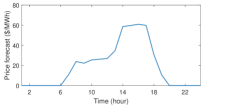
(a) Price forecast

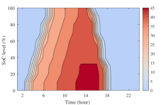
(b) Marginal value

Figure 2: Storage marginal value under price forecast. This case adopts a deterministic price forecast to demonstrate the monotonicity of storage marginal value.

5.2 Storage unbounded withholding

In this case study, we show that storage bidding behavior becomes unpredictable when faced with a price distribution with a fixed average but unlimited potential fluctuations.

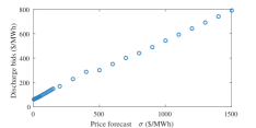
Figure 3: Storage unbounded discharge bids with fixed expectation and given deviations from 5 to 1500 $/MWh.

As shown in Figure 3, given storage price forecast follows a normal distribution with expectation as DAM price and deviation $\sigma$ from 0 to 1500 $/MWh. We observe that storage bids are monotonically increasing from 10 to 800 $/MWh, exceeding any reasonable limit. This finding, consistent with Theorem 1, highlights that price deviation plays a crucial role in shaping storage participation in the market. Storage units, seeking to hedge against potential price swings, bid aggressively when faced with high uncertainty, potentially leading to inefficient market outcomes. To address this issue and better align storage participation with social welfare, system operators could consider providing more transparent information about price forecasts or setting reasonable bounds on their potential fluctuations. This would help storage units make informed decisions and encourage more efficient capacity allocation within the market.

5.3 Storage bounded withholding

In this case study, we show that storage bids is bounded if the price forecast has a lower bound $\underline{\lambda}=$ 5 $/MWh and a high bound $\overline{\lambda}=$ 150 $/MWh. To demonstrate that Theorem 2 does not require specific price distribution, here we use a uniform distribution whose expectations are the same as Figure 2a, but the variances $\sigma_{t}^{2}$ increase from 5 to 400 $/MWh.

Our results in Figure 4 reveals that storage bounds and bids exhibit a dynamic relationship with deviations of the given distribution, in which the bids remain confined within the bounds outlined by equation (9a). We also find that due to the existence of upper and lower bounds, when deviation is larger than 200 $/MWh, storage bids will not increase as deviation increases, which differs from the results in Section 5.2. Therefore, we advocate for the system operator to establish price bounds that effectively regulate storage bids and bids while simultaneously ensuring societal welfare.

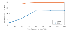
Figure 4: Storage bounded discharge bids with fixed expectation and deviations from 5 to 400 $/MWh.

5.4 Ideal case for welfare-aligned economic withholding

In this simulation, we investigate how storage incorporating price uncertainty can counteract system net demand uncertainties caused by real-time wind fluctuations.

To clearly show the findings of Corollary 6, we use a simplified setting with specific characteristics. First, we modify the ISO-NE test system from Krishnamurthy [37], by introducing a generator with infinite capacity and a quadratic cost function $G_{t}(g_{t})=10g_{t}+0.04(g_{t})^{2}$. Second, we consider both storage uncertainty and system uncertainty follow the same distribution. We model storage forecasts of RTM prices using normal distributions: Storage price forecasts centered around the DA price [35] with a deviation from 1 to 30 $/MWh. We then model the system uncertainty of net demand by considering RTM wind generation centered around the DA forecast with a deviation from 0.5 to 3 GW. System uncertainty is incorporated through a Monte-Carlo simulation with 200 realizations. Third, we incorporate storage capacity of 10 MW/40 MWh, a sufficiently small capacity that will not affect market clearing.

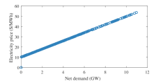
Figure 5: Relationship between market clearing price $\lambda_{t}$ and net demand.

Figure 5 demonstrates the RTM clearing price monotonically increasing with the standard deviation of the net demand, as predicted by Proposition 4. Due to the limited storage capacity, the storage price deviation is monotonically increasing with the market clearing price, which exhibits a linear relationship with the net demand.

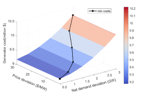
(a) Cost

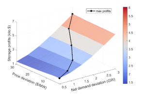
(b) Profit

Figure 6: Storage participation in markets under ideal case. This setup assumes minimal storage capacity within the system, alongside a single generator characterized by quadratic cost and infinite capacity. Then the storage uncertainty and system uncertainty are assumed to follow the same distribution.

Figure 6 reveals that the minimum cost and maximum profit points approximately lie along the diagonal of the map. This means the storage participants consideration of price uncertainty can counterpoise the system uncertainties, if the two uncertainties follows the same types of distributions. Note that, Corollary 6 suggests a linear relationship between storage uncertainty and system uncertainty, resulting in strict diagonally aligned points for minimum cost. Figure 6a exhibits slight differences from this ideal scenario. These differences can be attributed to 1) the discrete intervals used for both the $x$-axis (2 $/MWh) and $y$-axis (0.5 GW), 2) the limited number of Monte-Carlo realizations, and 3) the time-dependent dispatch characteristic of RTM. Notably, Corollary 6 focuses on a single period $t$, while simulation in this case involve storage’s SoC and charging/discharging decisions across multiple periods, influenced by the entire price prediction curve.

Moreover, in this case, due to limited storage capacity, storage participants possess near-perfect predictions of the market price. This results in the minimum cost and maximum profit points coinciding in Figure 6, indicating alignment between storage economic withholding and social welfare.

5.5 Practical case for welfare-aligned economic withholding

Real-word electricity markets have large difference from the ideal cases in the last section. First, the markets have a large number of generators with different cost functions. Second, the storage participants are not neglectable because increasing capacity integrated into markets. Third, the wind uncertainty is dependent on RT wind generation rather than a fixed value. For example, when daily wind generation varies from 0.1 GW to 10 GW,it is not reasonable assume wind generation has a fix deviation of 0.5 GW as we do in the last Section.

In this section, we bridge the gap between real-world electricity market and the ideal cases and study how storage withholding impact social welfare under real-world market settings as mentioned above. We employ the ISO-NE test system with 76 generators and consider storage capacity of 2.5 GW, which accounts for around 20% of the average load. For better representatives, we use the K-means approach to generate five representative demand and wind scenarios from the one-year data, in which the wind capacity is 26 GW with an average wind capacity factor of 0.4. We consider the wind uncertainty characterized by normal distribution whose expectation is DA wind generation, and deviation is proportional to DA wind generation as shown by the $x$-axis in Figures 7.

Figures 7a and 7b show the simulated cost and profit outcomes, respectively. Notably, the locations of minimum cost and maximum profit no longer coincide, although their trends remain aligned. This divergence arises from the clearing price deviating from forecasts due to three factors: increased storage capacity, multiple wind scenarios, and wind generation fluctuations.

Increasing storage capacity amplifies the impact of its charging and discharging actions on market clearing, leading to deviations from price forecasts. The multiple scenarios, representing low-wind and high-wind days, further contribute to uncertainty. Unlike the idealized case in Figure 6, where uncertainty directly maps to absolute deviation, the uncertainty on the $x$-axis in Figure 7 reflects a combination of wind generation variation and scenario weights.

On the positive side, Figure 7 reveals that the trend of the storage price forecast deviation aligns with the system cost and storage profit, suggesting that economic withholding can generally coincide with social welfare. However, this alignment is not guaranteed in all cases.

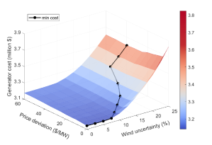
(a) Cost

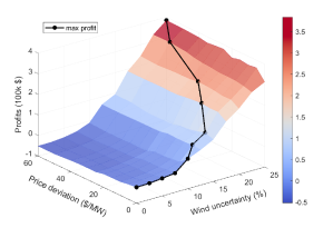
(b) Profit

Figure 7: Storage participation in markets under practical cases. This setup uses practical system settings of ISO-NE with 76 generators. Storage capacity accounts for 20% load, having a significant impact on market clearing. The results come from 5 representative demand and wind scenarios from the one-year data.

6 Conclusion

In this study, we proposed a novel strategy that incorporates uncertainty in price bidding for storage participating in a wind penetrated electricity market. We showed that a monotonic concave function that defines storage valuation, which reveals storage exercising of market power is limited because a higher SoC level will result in lower bidding prices. We also found that storage considering larger price uncertainty will result in higher storage capacity withholding. Based on the above findings, we demonstrate that uncertainty introduced into storage bidding could counterpoise the system uncertainties, the effect of this counterpoise is observed to impact the dispatch of all the distributed generators participating in the market and could potentially minimize the system costs and storage profits.

In conclusion, energy storage is not a market manipulator but an honest player contributing to the social welfare, if the system operator can share the information about renewable generation uncertainty. Crucially, we reveal that under certain conditions, the economic withholding behavior of storage can paradoxically enhance social welfare, especially when price models account for systemic uncertainties. This counterintuitive finding underscores the complexity of storage behavior in market dynamics. To substantiate our theoretical findings, we employ numerical simulations, including a case study modeled on the ISO New England system. These simulations provide empirical evidence supporting our theoretical predictions and offer insights into the practical implications of storage strategies in real-world electricity markets.

Appendix

6.1 Complete market simulation formulation

6.1.1 Optimization Model of Day-ahead Unit Commitment

This subsection provides a detailed description of the day-ahead dispatch model for unit commitment.

Based on the assumption of a single-storage system, the objective function of day-ahead unit commitment minimizes daily generation costs of fossil-fuel generators and the marginal discharge costs of energy storage:

$$\min_{g_{i,t},u_{i,t},y_{i,t},p_{t}} \sum_{t=1}^{T}\sum_{i=1}^{N_{g}}[G_{i,t}(g_{i,t})+c^{n}_{i}\cdot u_{i,t}+c^{s}_{i}\cdot y_{i,t}]$$

$$+\sum_{t=1}^{T}c\cdot p_{t}$$ (11a)

where $$g_{i,t} i t u_{i,t} i t y_{i,t} i t c^{n}_{i} c^{s}_{i} p_{t} j t N_{g}$$ is the electric power generation of fossil-fuel generator at period . is a binary variable indicating whether generator is on at period , and is a binary variable indicating whether generator turns on at period . is the generator no load cost, denotes generator start-up cost. is the storage discharging energy of participant at period , indicates the number of conventional generators.

The constraints are:

Generation minimum and maximum limits

$$\mathrm{Gmin}_{i}\cdot u_{i,t} \leq g_{i,t}\leq\mathrm{Gmax}_{i}\cdot u_{i,t},\$$ (11b)

where $\mathrm{Gmin}_{i}$ and $\mathrm{Gmax}_{i}$ denote the minimum and maximum generation of fossil-fuel generator $i$.

Generator ramping constraints

$$-\mathrm{RR}_{i} \leq g_{i,t}-g_{i,t-1}\leq\mathrm{RR}_{i}+\mathrm{Gmin}_{i}\cdot y_{i,t}\$$ (11c)

where $\mathrm{RR}_{i}$ is the ramp rate of generator $i$.

Generator start-up and shut-down logic constraints

$$y_{i,t}-z_{i,t} =u_{i,t}-u_{i,t-1}$$ (11d)

$$y_{i,t}+z_{i,t} \leq 1$$ (11e)

where $z_{i,t}$ is a binary variable indicating whether generator $i$ turns off at period $t$.

To address the real-time fluctuations caused by renewable generation, the power grid is required to have synchronous reserve capacity provided by thermal generators:

$$\sum_{i=1}^{N_{g}}r_{i,t} \geq(20\%)w_{t}$$ (11f)

$$r_{i,t} \leq\mathrm{Gmax}_{i}\cdot u_{i,t}-g_{i,t}$$ (11g)

$$r_{i,t} \leq RR_{i}$$ (11h)

where $w_{t}$ is accommodated wind generation during time period $t$, and $r_{i,t}$ is the reserve capacity.

Generator minimum up time constraint

$$\sum_{\tau=\max\{t-\mathrm{Tup}_{i}+1,1\}}^{t}y_{i,\tau} \leq u_{i,t}$$ (11i)

$$\sum_{\tau=\max\{t-\mathrm{Tdn}_{i}+1,1\}}^{t}z_{i,\tau} \leq 1-u_{i,t}$$ (11j)

where $\mathrm{Tup}_{i}$ and $\mathrm{Tdn}_{i}$ are the maximum up time and minimum down time of generator $i$, respectively.

Storage power rating constraints

$$0\leq b_{t}\leq P$$ (11k)

$$0\leq p_{t}\leq P$$ (11l)

$$b_{t} p_{t} t\in\{1,2,\dotsc,T\}$$ or is zero for any (11m)

where (11m) enforces that storage cannot charge and discharge during the same time period.

Storage SoC limits

$$e_{t}-e_{t-1}=-p_{t}/\eta+b_{t}\eta$$ (11n)

$$0\leq e_{t}\leq E\$$ (11o)

The electric power balance between the generation side and the load side

$$\sum_{i}g_{i,t}+w_{t}+\frac{1}{\Delta T}p_{t}=\hat{D}_{t}+\frac{1}{\Delta T}b_{t}$$ (11p)

where the dual variable $\lambda^{DA}_{t}$ associated with constraint (LABEL:gbalance) is the day-ahead electricity price at period $t$. $\Delta T$ indicates the time interval between two consecutive time periods. $\frac{1}{\Delta T}p_{t}$ and $\frac{1}{\Delta T}b_{t}$ indicates the discharge and charge power, respectively.

The wind generation limits

$$0\leq w_{t}\leq\hat{W}_{t}$$ (11q)

where $\hat{W}_{t}$ denotes the day-ahead wind generation forecast at period $t$.

Note that in equation (1), for clarity, we use $g_{t}$ to denote the vectors of $g_{i,t}$. Then $G_{t}=\sum_{i=1}^{N_{g}}G_{i,t}$.

6.1.2 Real-time Market Clearing

The real-time dispatch aims to minimize the generation costs of fossil-fuel generators and the opportunity costs of storage at time period $$t$$:

$$\min\sum_{i=1}^{N_{g}}G_{t,i}(g_{t,i})+O_{t}(p_{t})-B_{t}(b_{t})$$ (12a)

The remaining constraints are analogous to those in the day-ahead unit commitment model, but they are applied for each time period $t=1$, $t=2$, …, $t=T$ in the RTM dispatch:

$$\mathrm{Gmin}_{i}\cdot u_{i,t}\leq g_{i,t}\leq\mathrm{Gmax}_{i}\cdot u_{i,t}$$ (12b)

$$-\mathrm{RR}_{i}\leq g_{i,t}-g_{i,t-1}\leq\mathrm{RR}_{i}+\mathrm{Gmin}_{i}\cdot y_{i,t}$$ (12c)

$$\sum_{i}g_{i,t}+w_{t}+\frac{1}{\Delta T}p_{t}=D_{t}-d_{t}+\frac{1}{\Delta T}b_{t}:\lambda_{t}$$ (12d)

$$0\leq w_{t}\leq W_{t}$$ (12e)

$$0\leq p_{t}\leq P$$ (12f)

$$0\leq b_{t}\leq P$$ (12g)

$$p_{t} b_{t} t$$ or is zero at (12h)

$$e_{t}-e_{t-1}=-p_{t}/\eta+b_{t}\eta$$ (12i)

$$0\leq e_{t}\leq E\$$ (12j)

where $W_{t}$ is the real-time wind generation, which has deviations from day-ahead forecast $\tilde{W}_{t}$.

Constraints (12b) and (12c) set the power generation limits and the ramping limits of fossil-fuel generators, respectively. Note here $u_{i,t}$ and $y_{i,t}$ are known values from unit commitment results. Therefore, the real-time dispatch is a standard convex optimization problem with quadratic objective functions and linear constraints, which is efficient to solve. Constraint (12d) is the power balance constraint between the generation side and the demand side. Constraint (12e) indicates the wind generation should not exceed the wind capacity. Constraints (12f) and (12g) specify the limits on storage charging and discharging energy, respectively, and constraint (12h) ensures that storage cannot charge and discharge simultaneously during the same time period. Equation (12i) defines the relation between SoC level and charging/discharging energy, where $e_{t-1}$ is a known value, because results and states at $1,2,...,t-1$ have been obtained when executing real-time dispatch at period $t$. Constraint (12j) is the SoC limit at period $t$.

6.2 Proof of Proposition 2

Recall the definition of $V_{t}(e_{t})$ from Equation (2b), where $V_{t}(e_{t})=\mathbb{E}_{\hat{\lambda}_{t+1}}[Q_{t}(e_{t}|\hat{\lambda}_{t+1})]$. To establish the concavity of $V_{t}(e_{t})$, our goal is to demonstrate that the function $Q_{t}(e_{t})$ is concave. We commence the proof by considering the case for $t=T-1$, building upon the assumption that $V_{T}(e_{T})$ is a concave function.

To investigate the concavity of (2a), first consider the subdifferential of $Q_{T-1}(e_{T-1})$:

$\partial{Q_{T-1}}(e_{T-1})=\cap_{z\in\textbf{dom}Q_{T-1}}\{g|{Q_{T-1}}(z)\geq{Q_{T-1}}(e_{T-1})+g^{T}(z-e_{T-1})\}$

where $g$ is the subgradient.In the case when $Q_{T-1}(e_{T-1})$ is differentiable, we can express $g$ as:

$$g =\hat{\lambda}_{T}(\partialderivative{p_{T}}{e_{T-1}}-\partialderivative{b_{T}}{e_{T-1}})-c\partialderivative{p_{T}}{e_{T-1}}$$ (13)

$$\leavevmode\nobreak\ \leavevmode\nobreak\ \leavevmode\nobreak\ \leavevmode\nobreak\ +v_{T}(e_{T-1})\partialderivative{e_{T}}{e_{T}}$$

Note that $\hat{\lambda}_{t},\leavevmode\nobreak\ \forall t\in{1,2,...T}$ represents the price forecast of storage, independent of the state of charge (SoC) level $e_{t}$. Additionally, we leverage results from [12]:

$$\partialderivative{p_{t+1}}{e_{t}} =\begin{cases}0;\leavevmode\nobreak\ \leavevmode\nobreak\ \eqref{eq:c1}\text{ is binding}\\ \eta;\leavevmode\nobreak\ \leavevmode\nobreak\ \text{Otherwise}\end{cases}$$ (14a)

$$\partialderivative{b_{t+1}}{e_{t}} =\begin{cases}0;\leavevmode\nobreak\ \leavevmode\nobreak\ \eqref{eq:c2}\text{ is binding}\\ 1/\eta;\leavevmode\nobreak\ \leavevmode\nobreak\ \text{Otherwise}\end{cases}$$ (14b)

$$\partialderivative{e_{t+1}}{e_{t}} =\begin{cases}1;\leavevmode\nobreak\ \leavevmode\nobreak\ \eqref{eq:c1}\leavevmode\nobreak\ \text{or }\eqref{eq:c2}\leavevmode\nobreak\ \text{is binding}\\ 0;\leavevmode\nobreak\ \leavevmode\nobreak\ \text{Otherwise}\end{cases}$$ (14c)

Next, we examine all possible values of $g$, considering different binding conditions for constraints (2c) and (2d). We proceed by analyzing five cases:

• Case 1: $p_{T}=P$ and $b_{T}=0$. In this case, the battery is discharging at maximum power. The constraint (2c) is binding. Hence we can obtain $\partialderivative{p_{T}}{e_{T}}=0$ and $\partialderivative{b_{T}}{e_{T}}=0$. Consequently,

  $$g=v_{T}(e_{T})$$ (15a)

• Case 2: $p_{T}\neq P$ and $b_{T}=0$. In this case, the battery is only discharging between the lower and upper power boundaries, i.e., $0<p_{T}<P$. Constraint (2c) is not binding. Consequently,

  $$g=\eta(\hat{\lambda}_{T}-c)$$ (15b)

• Case 3: $p_{T}=0$ and $b_{T}=P$. This case is similar to case 1, where $b_{T}$ is at the upper boundary, and constraint (2d) is binding. Therefore, we have a similar result as Case 1.

  $$g\in\partial V_{T}(e_{T})$$ (15c)

  where $\partial V_{T}(e_{T})$ indicates the subdifferential of the convex function $V_{T}(e_{T})$.

• Case 4: $p_{T}=0$ and $b_{T}\neq P$. In this case, the battery is only charging between the lower and upper power boundaries, i.e, $0<b_{T}<P$. Constraint (2d) is not binding. Consequently,

  $$g=\frac{1}{\eta}\hat{\lambda}_{T}$$ (15d)

• Case 5: $p_{T}=0$ and $b_{T}=0$. In this case, the battery is neither charging nor discharging. Therefore,

  $$g\in\partial V_{T}(e_{T})$$ (15e)

Then we calculate the second-order subderivative of $Q_{T-1}(e_{T-1})$ based on the results of (15a)-(15e):

$${\partial^{2}Q_{T-1}(e_{T-1})}=\begin{cases}\{0\};\leavevmode\nobreak\ \leavevmode\nobreak\ \text{ Case 2, 4, and 5}\\ \partial^{2}V_{T}(e_{T});\leavevmode\nobreak\ \leavevmode\nobreak\ \text{ Case 1 and 3}\end{cases}$$ (16)

Given that $V_{T}(e_{T})$ is concave, we know $Q_{T-1}(e_{T-1})$ is concave under all given $\hat{\lambda}_{t}$. Therefore, $V_{T-1}(e_{T-1})$ is also concave. Recursively, we can conclude that $V_{T-2}(e_{T-2})$, $V_{T-3}(e_{T-3})$,…, $V_{1}(e_{1})$ are all concave, which finishes the proof.

6.3 Proof of Theorem 1

Theorem 1 says $v_{t}(0)$ is unbounded if price $\hat{\lambda}_{t+1}$ follows Gaussian distribution $N(\mu_{t+1},\sigma_{t+1})$ with fixed mean value $\mu_{t+1}$ and unbounded standard deviation $\sigma_{t+1}$.

To prove this theorem, we will show that $v_{t}(e)\geq 0$ is monotonically increasing with respect to $\sigma_{t+1}$ when $\sigma_{t+1}\geq\underline{\sigma}$. Thus, for arbitrary $\theta$, we can always find a $\sigma_{t+1}$ such that $v_{t}(0)\geq\theta$.

We first use the analytical expression of $q_{t}(e|\hat{\lambda}_{t+1})$ based on the result in [12]

$$q_{t}(e|\hat{\lambda}_{t+1})=$$ (17)

$$\leavevmode\nobreak\ \leavevmode\nobreak\ \begin{cases}v_{t+1}(e+P\eta)&\text{if $\hat{\lambda}_{t+1}\leq a_{1}(e)$}\\ \hat{\lambda}_{t+1}/\eta&\text{if $a_{1}(e)<\hat{\lambda}_{t+1}\leq a_{2}(e)$}\\ v_{t+1}(e)&\text{if $a_{2}(e)<\hat{\lambda}_{t+1}\leq a_{3}(e)$}\\ (\hat{\lambda}_{t+1}-c)\eta&\text{if $a_{3}(e)<\hat{\lambda}_{t+1}\leq a_{4}(e)$}\\ v_{t+1}(e-P/\eta)&\text{if $\hat{\lambda}_{t+1}>a_{4}(e)$}\end{cases}$$ (18)

where $a_{1}(e)=v_{t+1}(e+P\eta)\eta$, $a_{2}(e)=v_{t+1}(e)\eta$, $a_{3}(e)=[v_{t+1}(e)/\eta+c]^{+}$, and $a_{4}(e)=[v_{t+1}(e-P/\eta)/\eta+c]^{+}$ are parameter functions related to storage SoC $e$. Note that the expectation also holds after taking the derivative, hence

$$v_{t}(e) :=\mathbb{E}_{\hat{\lambda}_{t+1}\in\hat{\lambda}(\bm{\mu},\bm{\sigma}^{2})}\Big{[}q_{t}(e|\hat{\lambda}_{t+1})\Big{]}$$ (19)

Secondly, we obtain the analytical expression of $v_{t}(0)$. Following the results of Lemma 1, we know $q_{t}(0)$ is larger than zero. Considering the marginal value function $v_{t}(0)$ is the expectation of $q_{t}(0)$, we update (18) to the zero SoC level since the last term in the case conditions $e-P/\eta$ would not exist at zero SoC, hence

$$q_{t}(0|\hat{\lambda}_{t})=\begin{cases}v_{t+1}(P\eta)&\text{if $\hat{\lambda}_{t+1}\leq a_{1}(0)$}\\ \hat{\lambda}_{t+1}/\eta&\text{if $a_{1}(0)<\hat{\lambda}_{t+1}\leq a_{2}(0)$}\\ v_{t+1}(0)&\text{if $a_{2}(0)<\hat{\lambda}_{t+1}\leq a_{3}(0)$}\\ (\hat{\lambda}_{t+1}-c)\eta&\text{if $a_{3}(0)<\hat{\lambda}_{t+1}$}\end{cases}$$ (20)

where curve of $q_{t}(0|\hat{\lambda}_{t})$ is sketched in Figure 8.

Third, we show that $v_{t}(0)$ is monotonically increasing if $\sigma_{t+1}\geq\underline{\sigma}$, where $\underline{\sigma}$ is a constant at period $t+1$.

Given $q_{t}(0)$ in (20) is always positive, we can calculate

$$v_{t}(0) =\int_{-\infty}^{\infty}q_{t}(0|\hat{\lambda}_{t+1}=x)\cdot f_{\hat{\lambda}_{t+1}}(x)\leavevmode\nobreak\ dx$$

$$\geq\int_{c}^{+\infty}\frac{a_{1}(0)}{\eta}f_{\hat{\lambda}_{t+1}}(x)dx$$

$$\leavevmode\nobreak\ \leavevmode\nobreak\ +\int_{c}^{+\infty}\eta(x-c)f_{\hat{\lambda}_{t+1}}(x)dx$$ (21)

where $f_{\hat{\lambda}_{t+1}}(x)$ is the PDF function of price $\hat{\lambda}_{t+1}$. The two integral terms in (21) correspond to the red areas in Figure 8.

Then by calculating the derivative of the two integral terms in equation (21) with respect to $\sigma_{t+1}$, we know

$$\partialderivative{v_{t}(0)}{\sigma_{t+1}} \geq\frac{a_{1}(0)}{\eta}\cdot\frac{\mu_{t+1}-c}{\sigma_{t+1}}f_{\hat{\lambda}_{t+1}}(c)$$

$$\leavevmode\nobreak\ \leavevmode\nobreak\ \leavevmode\nobreak\ \leavevmode\nobreak\ -\frac{(\mu_{t+1}-c)(\mu_{t+1}+c)}{\sigma_{t+1}}f_{\hat{\lambda}_{t+1}}(c)$$

$$\leavevmode\nobreak\ \leavevmode\nobreak\ \leavevmode\nobreak\ \leavevmode\nobreak\ +\frac{(\mu_{t+1}-c)^{2}}{\sigma_{t+1}}f_{\hat{\lambda}_{t+1}}(c)+{\sigma_{t+1}}f_{\hat{\lambda}_{t+1}}(c)$$

$$=\frac{[(\frac{a_{1}(0)}{\eta}-2c)(\mu_{t+1}-c)+\sigma_{t+1}^{2}]f_{\hat{\lambda}_{t+1}}(c)}{\sigma_{t+1}}\leavevmode\nobreak\$$ (22)

If $(\frac{a_{1}(0)}{\eta}-2c)(\mu_{t+1}-c)\geq 0$, it is evident that $v_{t-1}(0)$ is monotonically increasing with $\sigma_{t+1}$. In this case, $\underline{\sigma}=0$.

If $(\frac{a_{1}(0)}{\eta}-2c)(\mu_{t+1}-c)<0$, we need the condition that $\sigma_{t+1}>\sqrt{-(\frac{a_{1}(0)}{\eta}-2c)(\mu_{t+1}-c)}$ to guarantee the right hand side of (22) larger than 0, making $v_{t}(0)$ monotonically increasing. In this case, we obtain that $\underline{\sigma}=\sqrt{-(\frac{a_{1}(0)}{\eta}-2c)(\mu_{t+1}-c)}$. Therefore, we can always find a $\underline{\sigma}$ that guarantees the monotone increasing of $v_{t}(0)$, which finishes the proof.

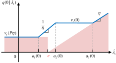
Figure 8: Curve of $q_{t+1}(0|\hat{\lambda})$. Note that $a_{1}(0)=v_{t+1}(P\eta)/\eta$ is positive according to Lemma 1.

6.4 Proof of Corollary 2

Our proof of Corollary 2 and the succeeding Corollary 3 buildings upon our previous results [38, 39] which provide an analytical update formulation of the value function as in (2b).

To prove that the value of $v_{t}(e)$ can become arbitrarily high with particular price distributions without changing the price expectation, we adopt the differential element method. We consider a price expectation $\hat{\lambda}_{t+1}$ and two alternative price values $\pi_{t+1}$ and $\gamma_{t+1}$ such that

$$\pi_{t+1}\geq\mu_{t+1}\geq\gamma_{t+1}$$ (23a)

that satisfy price distribution weights $\alpha_{t+1}>0$ and $\beta_{t+1}>0$ such that

$$\alpha_{t+1}\pi_{t+1}+\beta_{t+1}\gamma_{t+1} =\mu_{t+1}$$ (23b)

$$\alpha_{t+1}+\beta_{t+1} =1\;.$$ (23c)

Thus, we consider two price distributions with the same expectation $\mu$: 1) $\hat{\lambda}_{t+1}=\{\mu_{t+1}|f_{\hat{\lambda}_{t+1}}(\mu_{t+1})=1\}$; 2) $\hat{\lambda}_{t+1}=\{\pi_{t+1},\gamma_{t+1}|f_{\hat{\lambda}_{t+1}}(\pi_{t+1})=\alpha_{t+1},f_{\hat{\lambda}_{t+1}}(\gamma_{t+1})=\beta_{t+1}\}$. Our goal is thus to prove that given a $\mu_{t+1}$, there exist a set of $\pi_{t+1}$, $\gamma_{t+1}$, $\alpha_{t+1}$, and $\beta_{t+1}$ that satisfies (23a)–(23c) and

$$v_{t}(0)=\alpha_{t+1}q_{t}(0|\pi_{t+1})+\beta_{t+1}q_{t}(0|\gamma_{t+1})\geq\theta$$ (23d)

recall $\theta$ is our arbitrary bid value.

By observing (20) we see that given $\eta\in[0,1]$, $q_{t}(0)$ monotonically increases with $\hat{\lambda}_{t+1}$. Yet, the lowest value possible is bounded by $v_{t+1}(P\eta)$, but the high-value scales with $\hat{\lambda}_{t}$. Thus, we can reasonably set the lower price $\gamma_{t+1}$ to $v_{t+1}(P\eta)\eta$, and the high price value $\pi_{t+1}$ is at least greater than $[v_{t+1}(0)/\eta+c]^{+}$. Then substitute this into (23d), we have

$$\alpha_{t+1}(\pi_{t+1}-c)\eta+\beta_{t+1}v_{t+1}(P\eta) \geq\theta$$ (23e)

$$\frac{\theta-\beta_{t+1}v_{t+1}(P\eta)}{\alpha_{t+1}\eta}+c \leq\pi_{t+1}$$ (23f)

Then, summarizing our results, for an arbitrary real value $\theta$, the following price distribution will satisfy $v_{t}(0)\geq\theta$

$$f(\hat{\lambda}_{t+1})=\begin{cases}\beta_{t+1}\text{ if }\hat{\lambda}_{t+1}=v_{t+1}(P\eta)\\ \alpha_{t+1}\text{ if }\hat{\lambda}_{t+1}=\frac{\theta-\beta_{t+1}v_{t+1}(P\eta)}{\alpha_{t+1}\eta}+c\end{cases}$$ (23g)

while ensuring the price expectation is $\mu_{t+1}$ by satisfying (23a)–(23c). Hence we proved this Corollary.

6.5 Proof of Corollary 3

The proof also uses (18). In cases of $$e>P\eta \hat{\lambda}_{t+1}>[v_{t+1}(e-P/\eta)/\eta+c]^{+} \mu_{t}$$, a sufficient high price . We use the same pricing model as in (23a)–(23d) which ensures the price distribution mean is :

$$v_{t}(e)\geq\theta$$ (24a)

$$\alpha_{t+1}v_{t+1}(e-P/\eta)+\beta_{t+1}v_{t+1}(e+P\eta)\geq\theta$$ (24b)

$$v_{t+1}(e-P/\eta)\geq\frac{\theta-\beta_{t+1}v_{t+1}(e+P\eta)}{\alpha_{t+1}}$$ (24c)

Thus, using the assumed price distribution model to make the value function $$v_{t}(e) \theta v_{t+1}(e-P/\eta) e-P/\eta<0 t-\tau\geq e\eta/P$$ greater than , we need to ensure (24c), which states must be greater than a given value. Thus, recursively, by moving forward in time, we will reach in if . Then using Proposition 2, we can set the value function at zero SoC to any high values with a price distribution with fixed expectations.

Now we turn to Proposition 1, which shows the storage bids proportionally correlate with the value function derivative. Hence, we finished the proof.

6.6 Proof of Lemma 1

Assume storage duration is long enough that $2P\eta\leq E$. Given $v_{T}(e)\geq 0$, we can conclude that $v_{T}(0)\geq v_{T}(P\eta)\geq v_{T}(2P\eta)\geq v_{T}(E)\geq 0$, because $v_{t}(e_{t})$ is monotonically decreasing with respect to $e_{t}$.

Now let $t=T-1$, based on equation (20), we have

$$v_{t}(P\eta) =\int_{-\infty}^{\infty}q_{t}(P\eta|\hat{\lambda}_{t}=x)f(x)dx$$ (25)

$$=\int_{-\infty}^{v_{t+1}(2P\eta)\eta}v_{t+1}(2P\eta)f(x)dx$$

$$+\int_{v_{t+1}(2P\eta)\eta}^{v_{t+1}(P\eta)\eta}\frac{x}{\eta}f(x)dx$$

$$+\int_{v_{t+1}(P\eta)\eta}^{v_{t+1}(P\eta)/\eta+c}v_{t+1}(P\eta)f(x)dx$$

$$+\int_{v_{t+1}(P\eta)/\eta+c}^{v_{t+1}(0)/\eta+c}(x-c)\eta f(x)dx$$

$$+\int_{v_{t+1}(0)/\eta+c}^{\infty}v_{t+1}(0)f(x)dx$$

$$\geq\leavevmode\nobreak\ v_{t+1}(2P\eta)\int_{-\infty}^{v_{t+1}(2P\eta)\eta}f(x)dx$$

$$+v_{t+1}(2P\eta)\int_{v_{t+1}(2P\eta)\eta}^{v_{t+1}(P\eta)\eta}f(x)dx$$

$$+v_{t+1}(P\eta)\int_{v_{t+1}(P\eta)\eta}^{v_{t+1}(P\eta)/\eta+c}f(x)dx$$

$$+v_{t+1}(P\eta)\int_{v_{t+1}(P\eta)/\eta+c}^{v_{t+1}(0)/\eta+c}f(x)dx$$

$$+v_{t+1}(0)\int_{v_{t+1}(0)/\eta+c}^{\infty}f(x)dx$$

$$\geq\leavevmode\nobreak\ v_{t+1}(2P\eta)\geq 0,$$

By recursively applying equation (25) for time periods $t=T-1,T-2,...,1$, we establish the inequality $v_{t}(P\eta)\geq 0,\forall t\in\mathcal{T}^{{}^{\prime}}=\{1,2,3,...,T-1\}$. Hence we finish the proof.

6.7 Proof of Theorem 2

We follow the proof framework of Theorem 3. We update our price model to include the price bounds as

$$\overline{\lambda}\geq\pi_{t+1}\geq\mu_{t+1}\geq\gamma_{t+1}\geq\underline{\lambda}$$ (26a)

together the price model (23b)–(23c). Using the monotonic decreasing property from Proposition 2, we focus on $$v_{t}(0) v_{t}(0)$$ which has the highest value. Then, using (20), starting from the last time period with final SoC opportunity values, we can calculate as

$$v_{t}(0) =\alpha_{t+1}(\pi_{t+1}-c)\eta+\beta_{t+1}v_{t+1}(P\eta)$$ (26b)

$$=\frac{\mu_{t+1}-\gamma_{t+1}}{\pi_{t+1}-\gamma_{t+1}}(\pi_{t+1}-c)\eta$$

$$\leavevmode\nobreak\ \leavevmode\nobreak\ \leavevmode\nobreak\ \leavevmode\nobreak\ +\frac{\pi_{t+1}-\mu_{t+1}}{\pi_{t+1}-\gamma_{t+1}}v_{t+1}(P\eta)$$

$$=(\mu_{t+1}-\gamma_{t+1})\eta(1+\frac{\gamma_{t+1}-c}{\pi_{t+1}-\gamma_{t+1}})$$

$$\leavevmode\nobreak\ \leavevmode\nobreak\ \leavevmode\nobreak\ \leavevmode\nobreak\ +v_{t+1}(P\eta)(1+\frac{\gamma_{t+1}-\mu_{t+1}}{\pi_{t+1}-\gamma_{t+1}})$$

$$=(\mu_{t+1}-\gamma_{t+1})\eta+v_{t+1}(P\eta)$$

$$\leavevmode\nobreak\ \leavevmode\nobreak\ \leavevmode\nobreak\ \leavevmode\nobreak\ +\frac{(\mu_{t+1}-\gamma_{t+1})\eta(\gamma_{t+1}-c)}{\pi_{t+1}-\gamma_{t+1}}$$

$$\leavevmode\nobreak\ \leavevmode\nobreak\ \leavevmode\nobreak\ \leavevmode\nobreak\ +\frac{(v_{t+1}(P\eta)(\gamma_{t+1}-\mu_{t+1})}{\pi_{t+1}-\gamma_{t+1}}$$

Then given $$c\geq\gamma_{t+1} \mu_{t}\geq\gamma_{t+1} v_{t+1}(P\eta)\geq 0 \pi_{t+1} \gamma_{t+1} v_{t}(0) \pi_{t+1}=\overline{\lambda} \gamma_{t+1}=\underline{\lambda} v_{t+1}(P\eta)$$, and , (26b) is an increasing function to and a decreasing function to , hence value is maximized if and for all . Note that while we considered a price distribution model with only two realizations, we can generalize this result to all possible price distributions using the finite element methods by considering any price distribution as the sum of price pairs, as in (26a), then it is trivial to see in any sub-pair distribution models. The two price realizations will be at the price bounds.

According to the previous result, we can consider the following price process at period $t+1$: $f_{\hat{\lambda}_{t+1}}(\overline{\lambda})=\alpha_{t+1}$, $f_{\hat{\lambda}_{t+1}}(\underline{\lambda})=\beta_{t+1}$, with $\alpha_{t+1}+\beta_{t+1}=1$ and the expectation is $\mu_{t+1}$, will maximize $v_{t}(0)$ for any $v_{t+1}(P\eta)$. On the other hand, note the temporal transitive property of (18) that the value of $v_{t}(0)$ will be passed to $v_{t+1}(P\eta)$ in the previous time periods for high price results. Then $v_{t+1}(P\eta)$ becomes the input to the previous zero SoC value function. Hence, (26b) forms a recursive calculation with

$$v_{t}(0) =\alpha_{t+1}(\pi_{t+1}-c)\eta+\beta_{t+1}v_{t+1}(P\eta)$$

$$\leq\alpha_{t+1}(\pi_{t+1}-c)\eta+\beta_{t+1}v_{t+1}(0)$$

$$=\alpha_{t+1}(\pi_{t+1}-c)\eta$$ (26c)

$$\leavevmode\nobreak\ \leavevmode\nobreak\ \leavevmode\nobreak\ \leavevmode\nobreak\ \leavevmode\nobreak\ \leavevmode\nobreak\ \leavevmode\nobreak\ \leavevmode\nobreak\ +\beta_{t+1}\big{[}\alpha_{t+2}(\pi_{t+2}-c)\eta+\beta_{t+2}v_{t+2}(P\eta)\big{]}$$

$$=\dotsc$$

which provides the upper bound for the marginal value function $v_{t}(e)$. Then applying equation (3b) to design bids gives the result in (9a), hence finishing the proof.

6.8 Proof of Proposition 4

The idea of proving Proposition 4 is to demonstrate the RTM clearing price is monotonically increasing with respect to net demand.

For clarity, we first denote net demand $D_{t}-w_{t}=y_{t}$, then

$$L(g_{t},p_{t},b_{t},y_{t})$$

$$\leavevmode\nobreak\ \leavevmode\nobreak\ =G_{t}(g_{t})+O_{t}(p_{t})-B_{t}(b_{t})+\lambda_{t}(g_{t}+p_{t}-b_{t}-y_{t})$$ (27)

Now we consider net demand $y_{t}$ is a random variable independent from $g_{t},p_{t},b_{t}$. Given storage capacity is small enough, we can ignore the terms $O_{t}(p_{t})$ and $B_{t}(b_{t})$. According to the KKT condition and the derivative chain rule, we know

$$\partialderivative{L(g_{t},p_{t},b_{t},y_{t})}{y_{t}}\approx\partialderivative{G_{t}(g_{t})}{g_{t}}-\lambda_{t}=0$$ (28)

Therefore, we can take derivative of both sides of equation (28) using the derivative chain rule:

$$\partialderivative{\lambda_{t}}{y_{t}}=\frac{\partial^{2}G_{t}(g_{t})}{\partial g_{t}^{2}}$$ (29)

Considering functions $G_{t}(g_{t})$ is a convex function for all $t\in\mathcal{T}$, therefore, the second-order derivative is a non-negative constant, indicating the relationship between RTM price $\lambda_{t}$ and net demand $y_{t}$ is linear, which finishes the proof.

References

- [1] CAISO. Special report on battery storage (2023).
- [2] Larson, K. Battery stampede spurs sunny storage economics in ercot (2023).
- [3] US Energy Information Association. Form EIA-860 detailed data with previous form data (EIA-860A/860B) (2022).
- [4] Sioshansi, R. et al. Energy-storage modeling: State-of-the-art and future research directions. \JournalTitleIEEE Transactions on Power Systems 37, 860–875 (2021).
- [5] Kirschen, D. S. & Strbac, G. Fundamentals of power system economics (John Wiley & Sons, 2018).
- [6] Harvey, S. M. & Hogan, W. W. Market power and withholding. \JournalTitleHarvard Univ., Cambridge, MA (2001).
- [7] Zheng, N., Qin, X., Wu, D., Murtaugh, G. & Xu, B. Energy storage state-of-charge market model. \JournalTitleIEEE Transactions on Energy Markets, Policy and Regulation 1, 11–22 (2023).
- [8] Chen, C., Tong, L. & Guo, Y. Pricing energy storage in real-time market. In 2021 IEEE Power & Energy Society General Meeting (PESGM), 1–5 (IEEE, 2021).
- [9] Bansal, R. K., You, P., Gayme, D. F. & Mallada, E. A market mechanism for truthful bidding with energy storage. \JournalTitleElectric Power Systems Research 211, 108284 (2022).
- [10] CAISO. Caiso energy storage and distributed energy resources – storage default energy bid (2020).
- [11] Jkedrzejewski, A., Lago, J., Marcjasz, G. & Weron, R. Electricity price forecasting: The dawn of machine learning. \JournalTitleIEEE Power and Energy Magazine 20, 24–31 (2022).
- [12] Zheng, N., Jaworski, J. J. & Xu, B. Arbitraging variable efficiency energy storage using analytical stochastic dynamic programming. \JournalTitleIEEE Transactions on Power Systems (2022).
- [13] Jafari, M., Korpås, M. & Botterud, A. Power system decarbonization: Impacts of energy storage duration and interannual renewables variability. \JournalTitleRenewable Energy 156, 1171–1185 (2020).
- [14] Wang, B. & Hobbs, B. F. Real-time markets for flexiramp: A stochastic unit commitment-based analysis. \JournalTitleIEEE Transactions on Power Systems 31, 846–860 (2015).
- [15] Zhao, C. & Guan, Y. Data-driven stochastic unit commitment for integrating wind generation. \JournalTitleIEEE Transactions on Power Systems 31, 2587–2596 (2015).
- [16] Bertsimas, D., Litvinov, E., Sun, X. A., Zhao, J. & Zheng, T. Adaptive robust optimization for the security constrained unit commitment problem. \JournalTitleIEEE transactions on power systems 28, 52–63 (2012).
- [17] Lubin, M., Dvorkin, Y. & Backhaus, S. A robust approach to chance constrained optimal power flow with renewable generation. \JournalTitleIEEE Transactions on Power Systems 31, 3840–3849 (2015).
- [18] Ndrio, M., Madavan, A. N. & Bose, S. Pricing conditional value at risk-sensitive economic dispatch. In 2021 IEEE Power & Energy Society General Meeting (PESGM), 01–05 (IEEE, 2021).
- [19] Dvorkin, Y. A chance-constrained stochastic electricity market. \JournalTitleIEEE Transactions on Power Systems 35, 2993–3003 (2019).
- [20] Chattopadhyay, D. & Baldick, R. Unit commitment with probabilistic reserve. In 2002 IEEE Power Engineering Society Winter Meeting. Conference Proceedings (Cat. No. 02CH37309), vol. 1, 280–285 (IEEE, 2002).
- [21] Roald, L. A. et al. Power systems optimization under uncertainty: A review of methods and applications. \JournalTitleElectric Power Systems Research 214, 108725 (2023).
- [22] Bose, S. & Low, S. H. Some emerging challenges in electricity markets. \JournalTitleSmart grid control: Overview and research opportunities 29–45 (2019).
- [23] Rehman, S., Al-Hadhrami, L. M. & Alam, M. M. Pumped hydro energy storage system: A technological review. \JournalTitleRenewable and Sustainable Energy Reviews 44, 586–598 (2015).
- [24] Savkin, A. V., Khalid, M. & Agelidis, V. G. A constrained monotonic charging/discharging strategy for optimal capacity of battery energy storage supporting wind farms. \JournalTitleIEEE Transactions on Sustainable Energy 7, 1224–1231 (2016).
- [25] Krishnamurthy, D., Uckun, C., Zhou, Z., Thimmapuram, P. R. & Botterud, A. Energy storage arbitrage under day-ahead and real-time price uncertainty. \JournalTitleIEEE Transactions on Power Systems 33, 84–93 (2017).
- [26] Taylor, J. A., Mathieu, J. L., Callaway, D. S. & Poolla, K. Price and capacity competition in balancing markets with energy storage. \JournalTitleEnergy Systems 8, 169–197 (2017).
- [27] Zuluaga, T. V. & Oren, S. S. Data-driven sizing of co-located storage for uncertain renewable energy. \JournalTitleIEEE Transactions on Energy Markets, Policy and Regulation (2023).
- [28] Jiang, D. R. & Powell, W. B. Optimal hour-ahead bidding in the real-time electricity market with battery storage using approximate dynamic programming. \JournalTitleINFORMS Journal on Computing 27, 525–543 (2015).
- [29] Du, E. et al. Managing wind power uncertainty through strategic reserve purchasing. \JournalTitleIEEE Transactions on Power Systems 32, 2547–2559 (2016).
- [30] Ye, Y., Papadaskalopoulos, D., Moreira, R. & Strbac, G. Strategic capacity withholding by energy storage in electricity markets. In 2017 IEEE Manchester PowerTech, 1–6 (IEEE, 2017).
- [31] Nasrolahpour, E., Zareipour, H., Rosehart, W. D. & Kazempour, S. J. Bidding strategy for an energy storage facility. In 2016 Power Systems Computation Conference (PSCC), 1–7 (IEEE, 2016).
- [32] Wang, Y., Zhou, Z., Botterud, A. & Zhang, K. Optimal wind power uncertainty intervals for electricity market operation. \JournalTitleIEEE Transactions on Sustainable Energy 9, 199–210 (2017).
- [33] Qin, X., Xu, B., Lestas, I., Guo, Y. & Sun, H. The role of electricity market design for energy storage in cost-efficient decarbonization. \JournalTitleJoule (2023).
- [34] Gao, X., Knueven, B., Siirola, J. D., Miller, D. C. & Dowling, A. W. Multiscale simulation of integrated energy system and electricity market interactions. \JournalTitleApplied Energy 316, 119017 (2022).
- [35] Tang, W., Rajagopal, R., Poolla, K. & Varaiya, P. Model and data analysis of two-settlement electricity market with virtual bidding. In 2016 IEEE 55th Conference on Decision and Control (CDC), 6645–6650 (IEEE, 2016).
- [36] Dantzig, G. B. & Thapa, M. N. Linear programming: Theory and extensions, vol. 2 (Springer, 2003).
- [37] Krishnamurthy, D., Li, W. & Tesfatsion, L. An 8-zone test system based on iso new england data: Development and application. \JournalTitleIEEE Transactions on Power Systems 31, 234–246, 10.1109/TPWRS.2015.2399171 (2015).
- [38] Xu, B., Korpås, M. & Botterud, A. Operational valuation of energy storage under multi-stage price uncertainties. In 2020 59th IEEE Conference on Decision and Control (CDC), 55–60 (IEEE, 2020).
- [39] Zheng, N. & Xu, B. Impact of bidding and dispatch models over energy storage utilization in bulk power systems. \JournalTitleIREP Symposium on Bulk Power System Dynamics and Control 2022 (2022).