Non-robustness of diffusion estimates on networks with measurement error

Abstract.

Network diffusion models are used to study things like disease transmission, information spread, and technology adoption. However, small amounts of mismeasurement are extremely likely in the networks constructed to operationalize these models. We show that estimates of diffusions are highly non-robust to this measurement error. First, we show that even when measurement error is vanishingly small, such that the share of missed links is close to zero, forecasts about the extent of diffusion will greatly underestimate the truth. Second, a small mismeasurement in the identity of the initial seed generates a large shift in the locations of the expected diffusion path. We show that both of these results still hold when the vanishing measurement error is only local in nature. Such non-robustness in forecasting exists even under conditions where the basic reproductive number is consistently estimable. Possible solutions, such as estimating the measurement error or implementing widespread detection efforts, still face difficulties because the number of missed links is so small. Finally, we conduct Monte Carlo simulations on simulated networks, and real networks from three settings: travel data from the COVID-19 pandemic in the western US, a mobile phone marketing campaign in rural India, and an insurance experiment in China.

Researchers and policymakers studying the spread of ideas, technology, or disease often estimate models of diffusion using network data of how individuals interact. Examples include (i) quantifying the estimated extent of illness or technology take-up; (ii) summarizing diffusion dynamics (e.g., the reproduction number ${\mathcal{R}}_{0}$ of a disease); (iii) targeting interventions (e.g., where to seed new information to maximize spread, where to lockdown to prevent spread); (iv) and estimating counterfactuals (such as in estimates of peer effects, as we show in an empirical example). See Anderson and May, (1991), Jackson, (2009), Jackson and Yariv, (2011), and Sadler, (2023) and references within for all three classes of topics (as well as an account of how such models are used in the case of strategic behavior).

In this paper, we focus on a setting where the econometrician has imperfect measurement of either the interaction network or initial seeding, and wants to estimate models of diffusion or generate forecasts. Importantly, we let this measurement error be very small. In the case of a mismeasured network, only a vanishing proportion of links are missed asymptotically and nearly all links are observed. This captures the setting where an econometrician is equipped with the richest possible data on individuals and interactions, including geographic information such as residential data, schools and community centers, local markets, and local commuting information, and even mobile cell phone data tracking foot traffic.

We show that this tiny mismeasurement significantly affects the predictions of the econometrician’s estimated diffusion model. We show four key results: (i) predictions of diffusion counts can be arbitrarily incorrect with even vanishingly small measurement error of the network, (ii) predictions of diffusion counts can be arbitrarily sensitive to local uncertainty of the initial seeding; (iii) while aggregated estimated quantities such as the basic reproductive number ${\mathcal{R}}_{0}$ can be estimated correctly despite measurement error, it provides limited information for more disaggregated targets; (iv) because the measurement error is so small, most data augmentation (either estimating the measurement error or conducting additional data collection) will be ineffectual. In other words, if the measurement error is a needle in a haystack, it will be particularly costly and challenging to find the needle.

The key insight in our theoretical results is that settings with diffusion – where a process spreads as a function of contact with receptive individuals or units – are extremely susceptible to measurement error because missed links create opportunities for the process to propagate out of the econometrician’s view. This missed propagation creates knock-on effects that eventually overwhelm the econometricians’ estimated predictions.

To give intuition, consider a network where connections occur with a higher probability for people with some observable commonality (e.g., geography, school, work) or latent factors (e.g., Hoff et al., (2002)). This is common in many network formation models where dissimilarity between units decreases the probability of linkage. With a perfectly measured graph, when a diffusion process of information or disease is seeded, we can draw a ball around the initial seed that will exhaustively enumerate the number of nodes possibly affected by the process. This ball will expand over time, with the ball’s radius defined by the distance from the initial seed, and heavily influenced by the commonalities that affect peoples’ linking probability.

Now, consider a small set of idiosyncratic links that are missed in this network. If any of these missed links reach further than the ball drawn around the seed, the diffusion process can escape past the econometricians’ determined set of possibly impacted nodes. This set itself is small, but will have significant knock-on effects as the process quickly spreads outside of the ball. Since the link is outside of the ball, it spreads even more quickly because it has the largest possible set of unexposed units to diffuse to. This jump need not be far – it simply needs to be a link that creates diffusion unexpected by the econometrician. While we begin with the case of missing idiosyncratic links for simplicity, our general results allow each node to have potential mismeasurement to a vanishing share of nodes with an arbitrary distribution, and yet all aforementioned problems persist. This nests cases such as nodes only having missed links to a local neighborhood comprising a vanishing share of nodes; e.g., the measurement error is only allowed to be to a neighboring town and nothing more.

Missing links in the measurement of networks is a common concern (Wang et al.,, 2012; Sojourner,, 2013; Chandrasekhar and Lewis,, 2010; Advani and Malde,, 2018), but our paper highlights the dramatic impact of even the smallest errors when attempting to forecast diffusion. Mismeasurement can happen for several reasons. The first is practical: many analyses using empirical data (including one of our own empirical examples) do some amount of aggregation into groups with measured amounts of interaction. For example, individuals may be binned into groups of location-by-age-by-income, and the interactions between these groups are approximated based on underlying micro data. Using this data on individuals and interactions to construct compartments and forecast diffusion processes implicitly assumes that connections occur with a much higher probability for people with some observable commonality within the bin (Acemoglu et al.,, 2021; Farboodi et al.,, 2021; Fajgelbaum et al.,, 2021). Then, it may mismeasure cross-compartment connections. The choice of compartments may occur in order to smooth information and to have manageable “average” interaction patterns, but the connections across compartments will not capture the full heterogeneity of interactions.

Second, the mismeasurement of the network may occur because the sampling process for the network is imperfect. Studies surveying individuals may focus on local connections (e.g. within a school or village), and ignore other connections. Or, it may be that the network of potential meetings and connections is different from what is observed by many data sources. For example, cell phone data may provide a granular picture and yet omit a number of interactions that will play a crucial role in the diffusion process. Third, there is an intrinsic mismeasurement even with rich, static network data. Because the diffusion process evolves over time, a static snapshot of the network may not capture the relevant links for diffusion by the time the process reaches an individual.

In our theoretical analysis, we consider diffusion at its most disaggregated level, where the researcher estimates the interaction process at the unit level. We show that arbitrarily poor estimates can occur if the underlying interaction data carries even very small imperfections due to issues in the data sampling process. The lack of success in this setting is a conservative result that suggests compartmental models (which we consider in our empirical examples) will do just as badly. Compartmental models introduce a much larger volume of error, by smoothing over individual behavior to form compartments.

Formally, we study an asymptotic model in which parameters depend on the number of agents to tractably approximate finite-sample/time behavior, as is customary in graph theory. We consider a triangular array environment where there is a discrete set of $n$ agents who are in an undirected, unweighted network ${G}_{n}$. We take $n\rightarrow\infty$. A SIR (susceptible-infected-recovered) diffusion process proceeds for $T_{n}$ periods. Each period, a newly infected node passes the disease i.i.d. with probability $p_{n}$ and is then removed from the process. Since the model applies to diseases, technology adoption, social learning, and other diffusion settings, we use the term activated to nest the application-specific terms such as “infected,” “informed,” or “adopted” (Jackson and Yariv,, 2007).

We consider a time regime where it is neither early nor late. Extremely early on, there is almost no information and nothing has happened. Similarly, if we look far into the future, then the diffusion process saturates the network. Both cases make the problem uninteresting. So we work with the intermediate time regime, which is when estimators are developed, forecasts are made, and policy is designed. Formally, to approximate finite time behavior, we impose that $T_{n}$ is an increasing function of $n$. In addition to being tractable, it also embeds several intuitive assumptions. First, we impose upper bounds on $T_{n}$, in terms of functions of $n$, to ensure that the diffusion does not progress “too far.” This rules out cases where the diffusion covers (approximately) the entire graph, as the process is able to reach the edge of the graph. Second, we impose lower bounds on $T_{n}$, again in terms of functions of $n$ to rule out the initial periods where all diffusion is extremely local to the initial seed and measurement error will not play a role (unless the measurement error is extreme). The resulting asymptotic framework applies to any $T_{n}$ that falls within the given bounds, which are determined from the structure of the model.

We define the true network over which the diffusion process spreads as $G_{n}=L_{n}\cup E_{n}$. The subgraph $L_{n}$ is fully observed by the econometrician and is deterministic, while $E_{n}$ is an unobserved stochastic error graph. This setup corresponds to an econometrician taking a sample from $G_{n}$ and observing (without error) $L_{n}$. In practice, this could mean, for example, using a graph constructed from cell phone call logs as the true interaction graph. As discussed below, we assume that $L_{n}$ is very close to a complete sample from $G_{n}$ – so close that uncovering the additional missing edges in $E_{n}$ is impossible with realistic data collection strategies. Motivated by the empirical and statistical literature, we assume that the diffusion process on $L_{n}$ has a predominantly polynomial expansion structure in our main results, which generalizes a local meeting topology (e.g., geography, social groups). This setup nests any finite-dimensional Euclidean model, including but not limited to geographic networks, Euclidean networks, lattices, latent space models on Riemannian manifolds of weakly positive curvature, and so on, but the term geographic provides a useful intuition. Importantly, our assumption of polynomial expansion of the diffusion does not require polynomial expansion of the underlying graph, nor are our results limited to the polynomial case. We consider polynomial expansion because it reflects the common empirical analogs used in the data. We cover the exponential case for completeness, characterizing when measurement error is problematic despite the more rapid expansion. The exponential case covers the entire graph more rapidly, shrinking the set of $T_{n}$ sequences in which our analysis applies.

The error graph $E_{n}$ contains idiosyncratic links that, in our baseline model, are drawn i.i.d. with probability $\beta_{n}$ amongst all pairs of nodes. Crucially, we assume that in the limit essentially all of the links in the true network $G_{n}$ come from $L_{n}$. That is, $|E_{n}|/|L_{n}|\rightarrow_{p}0$. We assume an even stronger upper bound on the rate so that no giant component can form in $E_{n}$: $\beta_{n}=o(1/n)$. Therefore the pathologies we identify due to mismeasurement cannot be a function of a large unobserved component of spread.

We assume that the econometrician collects data and observes the network $L_{n}$. Since the econometrician has perfect knowledge of $L_{n}$, approximating data collection that is near-perfect for $G_{n}$, $E_{n}$ is the only source of measurement error. In much of our analysis, the initial seed $i_{0}$ is also known exactly to the econometrician. Collectively, these are strong assumptions that work in favor of the econometrician, reflecting a best-case scenario.

We begin by looking at forecasting difficulties in Section 2. Theorem 1 shows that the econometrician’s estimates of the diffusion count will be of lower order of magnitude than the true counts in the intermediate run (after the very initial periods, and before the disease saturates the entire network). In other words, the prediction will be dominated by the error. Very few idiosyncratic links are necessary for this phenomenon. A key conceptual point is that the idiosyncratic links do not shift the polynomial expansion of the diffusion to an exponential – rather, they increase the polynomial degree.

Second, in Theorem 2, we show that diffusion on $G_{n}$ – even when the error network is completely known – is not stable. This concretely captures the idea that perturbing the initial seed inside a small town when studying the overall spread at the state level can lead to massive differences in who is activated (i.e., infected, informed, or has adopted, based on application) and where they are in the state. Formally, we define a sequence of neighborhoods about $i_{0}$, $U_{n,i_{0}}$, to be local relative to the diffusion if the size of the neighborhoods vanishes relative to $B_{i_{0}}(T)$ (the set of all possible nodes activated from $i_{0}$ by time $T$). We show that over the time horizons of interest, there is some set $J_{n,i_{0}}$ that can be constructed which is a non-vanishing share of $U_{n,i_{0}}$ such that seeding with $j_{0}\in J_{n,i_{0}}$ rather than $i_{0}$ can lead to numerous disparate regions being diffused to and large disagreement in who is activated. This property holds even when the entire $G_{n}$ is perfectly known to the policymaker.

In Section 3.1, we turn to the problem of estimating the parameters of the diffusion process. The simple point is that one can consistently estimate both the diffusion parameter $p_{n}$ and the basic reproduction number ${\mathcal{R}}_{0}(G_{n})$ in a straightforward manner. Common intuition would suggest that equipped with these quantities, one could have a feel for where and how virulently the diffusion spreads to disparate regions. Yet we find that forecasts can become arbitrarily inaccurate, and exhibit sensitive dependence on the initial seeding of the diffusion process. While ${\mathcal{R}}_{0}$ captures the aggregate behavior of the diffusion, extending it to more disaggregated estimands is a challenging task.

We consider two possible solutions in Section 3.2: (i) estimating the idiosyncratic links through supplementary data collection and (ii) widespread node-level sampling (e.g., testing). In our assumed regime neither solution works. First, consider the case where the econometrician estimates $\beta_{n}$ and uses this information. We show that when the econometrician samples the population in a reasonable manner to obtain a large sample to estimate the volume of unobserved, idiosyncratic links, they will be unable to consistently estimate $\beta_{n}$. In fact, with large samples of nodes (on the order of $\sqrt{n}$), the probability of observing no idiosyncratic link in a supplemental survey tends to one (so $\hat{\beta}=0$ identically). Even with unrealistically large survey samples, close to order $n$ itself, the estimators will likely be inconsistent. Despite not being able to measure the error rate, it is large enough to cause severe forecasting problems.

The second possible solution is to look at when the policymaker uses widespread node-level sampling (e.g., testing) to detect what regions in society have activated agents. Specifically, the policymaker thinks of society as comprised of a number of regions — mutually exclusive connected sets of nodes in $L_{n}$ — and attempts to estimate which regions of society currently have activated agents. We assume that the policymaker detects every activated agent with i.i.d. probability $\alpha$. In an informational setting, this might reflect the quality of a survey elicitation. In the epidemic setting, this will involve the power of the biological test. In both settings, $\alpha$ also involves the yield rate for the sample including non-response and non-consent. The natural intuition is that with many draws, since the policy maker attempts to sample all nodes (so the effective power to detect is $\alpha$), the share of regions with activated agents that are detected as currently having activated agents should be large and at least $\alpha$. In Theorem 3, we show that the opposite holds. Namely, even with very sparse idiosyncratic links, the misemeasurement makes it such that the share of regions that have activated nodes that are actually marked correctly is at most $\alpha$. The intuition is that even when $\beta_{n}$ is very low, newly activated regions have so few activated agents that they may not be detected, and pushing this calculation forward shows that this will be the case for many such regions.

Section 4 contains our strongest result. It generalizes the preceding results and makes clear that they do not rely on the assumption that $E_{n}$ is comprised of idiosyncratic links between any two nodes with some i.i.d. probability. This is a convenient notational device to write rates in a clear way, depending only on restrictions of $\beta_{n}$, the error rate, without introducing a second concept: the allowable set of mismeasurements. In practice, one can even allow for models where $\beta_{ij,n}$ varies at the pair level; we study a structure of measurement error where every $i$ only has possible links in $E_{n}$ to a vanishing share of nodes in $n$: $\beta_{ij,n}\neq 0$ for a vanishing share of $j$s. This nests the case in a “geographic” setting where $i$ is only allowed to have these missed links “locally” in a ball around $i$. Despite this very general structure on both the shape of mismeasurement and how limited its domain can be, all of the aforementioned results carry through. We note that in the case where the share of nodes that can be linked to diminishes at a sufficiently fast rate, our results no longer apply.

We formalize this in Theorem 4 and Corollary 1. This generalization is particularly important because it makes clear that the forecasting and robustness failures we identify are not a product of missing “long-range shortcuts” that generate “small worlds.” It can be the case that the only kinds of links that are missed are those which were restricted to a small set of other nodes and which are highly localized in geographic-type models. The force that underlies the robustness failure is not about a few very surprising, long-range links, but instead is about the sheer accumulation of “re-seedings” that are missed, irrespective of the configurations of these misses.

Section 5 contains an extension for completeness. We consider the case wherein the econometricians’ dataset exhibits exponential expansion. Clearly, with exponential expansion, the diffusion saturates the network incredibly quickly, rendering the forecasting problem moot. Nonetheless, exponential expansion in $L_{n}$ could be because the underlying interaction data contains non-local mavens and non-local heavy tails of interactions and this information is known to the econometrician. For example, if the econometrician could perfectly forecast all future super-spreader events, this would be the case. Surprisingly, even in this case, it is possible to mis-forecast the diffusion, albeit under a stronger bound on idiosyncratic links. Theorem 5 shows that forecasts are not accurate when $E_{n}$ contains a large component—that is, $E_{n}$ must contain a component that contains a constant fraction of the $n$ nodes.

In simulation, we first examine versions of our main theorems. We directly simulate a diffusion process on both simulated and real-world networks with and without measurement error. In our Monte Carlo exercises, we generate different networks that match features such as degree and clustering in known empirical data. We set the measurement error probability to be quite small ($\beta_{n}\approx 1/10n$) and find that forecasts are problematic even with such small measurement error: underestimates of the diffusion count range from 22% to 83% across the simulations. We also demonstrate extreme sensitivity to initial conditions. Our first example shows that even when we perturb the initial seed in a neighborhood comprising 1% of the graph, 31% of the counterfactual seeds in this neighborhood would generate large failures of predictability of who is activated downstream. We find the expected overlap share of activated nodes over perturbations is only 40% by the time the diffusion could potentially have saturated the network. If we perturb in a 5% neighborhood, then 65% of the neighborhood is counterfactually problematic and then by the time of saturation the overlap percent is only 13%.

As an additional exercise, we fit a simple compartmental SIR model—a continuous time, continuum of agents mean-field approximation—to the generated diffusion data. We explore deviations when the (actual) diffusion process, comprised of discrete agents over discrete time, is approximated through the compartmental SIR model. We find that graphs with higher dimensional diffusion processes can be well approximated “in sample” (data used to estimate the model and build forecasts) by the compartmental SIR model, while lower dimension processes cannot. Further, in both cases, the fitted compartmental model forecasts a much earlier acceleration of diffusion relative to the actual diffusion process. Moreover, the compartmental model predicts at times a dramatically lower overall number of activations.

We then turn to exercises using observed data. In our first example, using location data from California and Nevada, we construct a real-world mobility network and examine network mismeasurement due to “pruning” – where links between locations are only included if a sufficient number of people move between them. We find that changing the threshold from five to six people traveling between Census tracts causes the policymaker to underestimate the extent of diffusion by nearly 56 percentage points. If instead of pruning, we induce errors by removing i.i.d. random links (holding fixed the volume of missed links), we find even more extreme underestimation: the policymaker underestimates the extent of diffusion by more than 76 percentage points. In addition, in both cases, there is little spatial overlap between epidemics when we perturb the initial location by only three links in the graph. As a second example, we turn to a viral marketing experiment in rural India (Banerjee et al.,, 2019). We show that similar patterns hold. When we add links with i.i.d. probability $\beta_{n}\approx 1/400$ in village networks with 200 nodes, the econometrician underestimates diffusion by nearly 15 percentage points. We also document extreme sensitive dependence on the seed set: we move only one single seed (out of up to five seeds in a village) to one of its neighbors, and we find that the resulting diffusion patterns always have distinctions in terms of which nodes are activated. On average across simulations, the intersection of activations starting at the highly similar seeds is only 61 percent of the activations encompassed by both diffusions.

As a final empirical example, we turn to the problem of estimating peer effects. We motivate the connection by considering a peer effects regression based on a diffusion measure. Using data from Cai et al., (2015), we estimate a regression and show that the estimates are sensitive to the network specification. We consider i.i.d. errors that correspond to at most missing one in five links, and show that it leads to dramatic loss of power – we find that the econometrician fails to reject the null under 15% of simulation draws, despite the null being false. While the bias is relatively small on average, any given realization of the network can generate large changes in the coefficient values.

Together, this set of results generates broader implications. For instance, a potential corollary is that compartmental SIR models used to approximate a diffusion process may suffer the aforementioned problems as they generate such mismeasurement from ignoring small leakages across compartments. Our results also have implications for policy design in situations where diffusion plays an important role. Given the forecasting difficulties, we expect that estimated optimal policies may change dramatically depending on the network data collected.

1. Model

1.1. Environment

We model society through a sequence of (random) undirected, unweighted graph $G_{n}$, indexed by the number of nodes $n$. $G_{n}$ is constructed as follows. There is a sequence of “base” graphs, $L_{n}$, with minimum degree $d_{L}$. We assume that $L_{n}$ is undirected, unweighted, and connected. Then the full social network is given by $G_{n}:=L_{n}\cup E_{n}$, which is the union of the “base” $L_{n}$ and where $E_{n}$ is a collection of random links. We assume that the policymaker perfectly observes (samples) only the base graph $L_{n}$; in that sense, $E_{n}$ can be thought of as an error graph. The links in $E_{n}$ are formed with i.i.d. probability $\beta_{n}$ between each pair of nodes. There is a diffusion process that spreads over the network $G_{n}$ following a standard SIR process with i.i.d. passing probability $p_{n}$.

It is useful to define $P_{n}(G_{n})$ as a percolation on the graph $G_{n}$. This is a directed, binary graph with each link activated i.i.d. with probability $p_{n}$. The SIR process we study is equivalent to a deterministic process emanating from some initial seed through $P_{n}(G_{n})$.

We conduct asymptotic analysis, taking limits as both $T$, the number of time periods, and $n$, the number of nodes becomes large. Formally, we will consider a sequence of graphs $\{L_{n},E_{n}\}$, where $E_{n}$ are drawn randomly, that grows with $n$, and consider $T:=T(n)$ where $T$ is an increasing function in $n$. More precision on exactly how $T$ grows is discussed below. We will generally suppress the dependence of $T$ on $n$ for ease of notation.

As a matter of notation, let $B_{j}(t)$ denote the ball of radius $t$ around vertex $j$ in a given graph and let $\{X_{n}\}_{n}=(X_{1},\ldots,X_{n},\ldots)$ denote the sequence of (possibly random) variables $X_{n}$.

We define the expected activation set as

$${\mathcal{E}}_{t}={\mathbb{E}}\left|\{x\in L_{n}\mid x\textrm{ ever activated by the diffusion on }L_{n}\}\right|,$$

that “activated” could mean “infected,” “informed,” “adopted,” etc., depending on application. To set up our first results, we impose the following condition on the diffusion process.

Assumption 1 (Polynomial Diffusion Process).

For some constant $q>1$ and all discrete time $t$, ${\mathcal{E}}_{t}=\Theta(t^{q+1})$ and ${\mathcal{S}}_{t}={\mathcal{E}}_{t}-{\mathcal{E}}_{t-1}=\Theta(t^{q})$. Furthermore, $p_{n}\in\left(\left(\frac{1}{\log n}\right)^{\frac{q}{2q+2}},1\right]$.

We write this assumption over the diffusion process rather than on the graph structure of $L_{n}$ to allow for more generality. We could have simply assumed that $L_{n}$ itself has polynomial expansion, and together with the appropriate $p_{n}$ and i.i.d. draw assumptions, Assumption 1 follows. But, we also allow for more general settings. For example, Assumption 1 covers cases of $L_{n}$ with non-polynomial expansion and i.i.d. draws of $p_{n}$, but with a sub-critical passing probability or short time horizons. The lower bound on $p_{n}$ is to ensure that the diffusion process spreads with sufficient speed – otherwise, the diffusion may halt before the medium time horizon that we study.

Turning to the substance of the assumption itself, first note that this condition implies that as the diffusion progresses, a growing number of nodes become activated in expectation. Second, this condition governs both the structure of the graph and the diffusion process. As an example, consider a latent space network where nodes form links locally in a Euclidean space (Hoff et al.,, 2002). Since volumes in Euclidean space expand at a polynomial rate, this ensures that Assumption 1 will be satisfied. Third, note the geometric relationship between ${\mathcal{E}}_{t}$ and ${\mathcal{S}}_{t}$ — ${\mathcal{E}}_{t}$ governs the total volumetric expansion of the diffusion, while ${\mathcal{S}}_{t}$ governs the shells of the diffusion (e.g., the boundary at time $t$). We explore the case where ${\mathcal{E}}_{t}$ has exponential growth for completeness in Section 5.

We next put specific constraints on the time horizon considered. The first condition restricts the time so that the diffusion has not reached the edge of the graph. The second condition contains two substantive points: first, it is a mechanical assumption to ensure that under Assumption 3, there are links in $E_{n}$ in expectation. The second condition also ensures that we are making a forecast about a time that is appreciably far enough in the future, so idiosyncratic links that are missed have a chance to play a role. Note that our results will hold for any $T_{n}\in[\underline{T}_{n},\overline{T}_{n}]$.

Assumption 2 (Forecast Period).

We impose that the sequence $T_{n}$ has for each $n$, $T_{n}\in[\underline{T}_{n},\overline{T}_{n}]$ where the following holds:

1. $\overline{T}_{n}=n^{\frac{1}{q+1}}$

2. $\underline{T}_{n}=(p_{n}\log n)^{\frac{1}{q+2}}$.

While $p_{n}$ can go to zero under Assumption 1, the lower bound on $p_{n}$ rules out the case where $\underline{T}_{n}\rightarrow 0$ as $n\rightarrow\infty$. The intuition for why $p_{n}$ plays a role in the time bound is that we need enough diffusion for the result to hold.

1.2. Econometrician’s Forecasting Problem

The econometrician’s policy objective is to estimate the expected number of activated (e.g., infected, informed, adopted, etc., based on application) nodes by date $T$. We assume they observe $L_{n}$ and treat it as their estimate of $G_{n}$. They also know the initial seed $i_{0}$ (an assumption we relax later on). Without loss of generality, we assume the econometrician’s problem begins at period $t=0$ and their objective is to predict the extent of diffusion at some period $T$. Note that perfect knowledge of $L_{n}$, knowledge of the initial seed, and knowledge of the start time are all strong assumptions that help the econometrician. Therefore, our first result can be thought of as modeling the policy objective in a best-case scenario. We later relax the assumption of perfect knowledge of the location of $i_{0}$ and consider the instability of the process to perturbations of the initial seed.

Let $y_{jt}$ be an indicator which denotes if node $j$ has ever been activated through time $t$. In principle the target estimand is

$$\hat{Y}_{T}(G_{n}):={\mathbb{E}}_{E_{n},P_{n}(G_{n})}\left[\sum_{j=1}^{n}y_{jT}\;\bigg{\rvert}\;L_{n}\right]$$

where the expectation is taken with respect to the diffusion process $P_{n}(G_{n})$ on graph $G_{n}$ and realizations of $E_{n}$, with known $i_{0}$. However, the econometrician uses only the observed $L_{n}$ as a stand-in (or mistakenly views this as the actual network driving diffusion),

$$\hat{Y}_{T}(L_{n}):={\mathbb{E}}_{P_{n}(L_{n})}\left[\sum_{j=1}^{n}y_{jT}\;\bigg{\rvert}\;L_{n}\right]$$

where the expectation is taken with respect to the diffusion process $P_{n}(L_{n})$ on $L_{n}$ (mistakenly assuming $E_{n}\equiv 0$) with known $i_{0}$.

1.3. Measurement Error

We impose bounds on $\beta_{n}$, the rate at which idiosyncratic links form.

Assumption 3.

$\beta_{n}\in\left(\frac{1}{p_{n}nT^{q}},\frac{1}{n}\right)$

Note that, first, both the upper and lower bounds go to zero as both $n$ and $T$ grow large. Second, by Assumptions 1 and 2, $p_{n}T^{q}\geq 1$. Third, it ensures that the missing links that are unobserved by the econometrician are small relative to the observed links, in the following sense: with probability one, $E_{n}$ is not a connected graph, nor will it contain a giant component as $n\rightarrow\infty$. This means that the large forecast errors we characterize below is not a function of a dense set of missing links, but instead, caused by a small (and disconnected) set of idiosyncratic links. While the forecast errors would also clearly happen if the econometrician missed a dense graph or a giant component, we focus on a regime where the mismeasurement is sparse, making the results more surprising.

2. Forecasting Difficulties

We now show how tiny measurement error leads to large forecasting errors in the diffusion process. First, we show how using the observed network $L_{n}$ to make forecasts with a known seed can greatly underestimate the average extent of diffusion on the true network $G_{n}$. Second, we show how diffusion patterns can be very different even with small perturbations to the location of the initial seed, even when the true graph $G_{n}$ is known without measurement error.

2.1. Forecasting errors given a known seed

We begin by studying the case where the policymaker has knowledge of both the observed network $L_{n}$ and the initial seed location of $i_{0}$. However, despite these advantages, we show that the econometrician’s forecast error will swamp the forecast as $n\to\infty$.

Theorem 1.

Under Assumptions 1, 2, and 3, as $n\rightarrow\infty$, $\frac{\hat{Y}_{T}(L_{n})}{\hat{Y}_{T}(G_{n})}\rightarrow 0.$

All proofs are in Appendix A unless otherwise noted.

We briefly give some intuition of why the forecast error dominates the predicted error in magnitude. Small errors caused by the error network $E_{n}$ recursively compound on themselves, creating massive forecast error. When considering the diffusion process in period $t$, it is helpful to consider a volume around the initial node (what we call a “shell”) of size $t$. This shell contains all the nodes that could possibly be activated by the process according to our observed network, $L_{n}$. As time grows, this shell grows in size, and as one might expect, the likelihood of hitting a low probability mismeasured link in $E_{n}$ increases. This leads to the creation of a new shell elsewhere on the graph. This initial missed jump to other locations in the network does not generate forecasting issues of any consequence. What creates the issue is that these jumps recursively explode. In totality, these new shells caused by the propagating error dwarf the diffusion captured by the observed graph $L_{n}$.

The proof strategy formalizes this intuition. We first compute a lower bound on the number of expected new “shells” in each time period. To generate a lower bound on expected activations, we introduce a tiling of the graph and count how many tiles are activated in expectation. We then calculate this number and scale by the number of nodes activated in each tile.

In Appendix F, we prove a similar version of Theorem 1 that allows the diffusion process to slow over time. We consider the case where the diffusion process decays at a polynomial rate: the resulting structure is equivalent to considering a diffusion process with a lower $q$. Doing so requires slightly different assumptions: we require an earlier time window and a higher rate of missing links. The intuition is that we need additional missing links to “compensate” for the slowing diffusion process to get the same result.

In the above analysis, the policymaker is agnostic to the location of diffusion, which may not be realistic in practice. A key consequence of our result, which follows from the proof strategy, is that we assume the policymaker perfectly forecasts the diffusion locally around the initial seed. We decompose the forecast based on $G_{n}$ into two components: the spread from $i_{0}$ through $L_{n}$, and activation waves “seeded” through links in $E_{n}$. Locally, the policymaker has a perfect forecast of exactly ${\mathcal{E}}_{t}$. In reality, the policymaker likely has errors locally as well and perhaps more so than globally, a concept we explore in greater depth in Section 4.

2.2. Sensitive Dependence on the Seed Set

We next consider the assumption that the policymaker has perfect knowledge of $i_{0}$ and show the sensitivity of the process depending on which nodes start the diffusion. This result shows an additional limit of the econometrician’s forecasting ability. Here, we assume that $G_{n}$ is perfectly observed, removing any sense of measurement error in the network, and consider variation in different seeds (the initially activated nodes). We make this comparison to show a structural lack of robustness of this model, potentially caused by mismeasurement in the initial seed: if seeds differ only slightly, this is enough to generate very different diffusion patterns.

The setup of the result is motivated by a policy-relevant consideration. If the policymaker is slightly incorrect in their assessment of the seed (e.g., patient zero), do we see large differences as to both where the diffusion jumps and who is activated? Here, we give the policymaker the advantage of knowing $G_{n}$ and facing no measurement error. While there are idiosyncratic links in $E_{n}$, the policymaker observes them. Despite these advantages, the policymaker will still encounter problems.

We fix a baseline percolation, $P_{n}$, for the diffusion process and vary only the initial seed of the process between $i_{0}$ and some neighboring $j_{0}$. This removes the randomness from the diffusion and holds fixed the set of possible paths that it can take as we vary the initial seed. The percolation is a useful construct because we can study the resulting activated sets, given percolation $P$, when seeding with some $i_{0}$ versus some $j_{0}$. Let $I_{P}(i_{0},T)$ and $I_{P}(j_{0},T)$ denote the ever-activated sets by period $T$ for the two seeds respectively. This holds the counterfactual passing process across each link fixed as we look across different initial seeds.

It is useful to define a catchment region. For some node $e$ that is activated at time $t$, if the diffusion process continues for $T$ more periods, then the catchment area is the maximal set of nodes that can be indirectly activated beginning with $e$, $B_{e}(T)$. In what follows, we will find that, given the extreme sparsity of $E_{n}$, for any two nodes $e_{1}$ and $e_{2}$ which have edges in $E_{n}$ (i.e., there exists alters $e_{1}^{\prime},e_{2}^{\prime}$ that $e_{1}e_{1}^{\prime},\ e_{2}e_{2}^{\prime}\in E_{n}$), the catchment areas (over $t$ periods of transmission) typically will not intersect: $B_{e_{1}^{\prime}}(t)\cap B_{e_{2}^{\prime}}(t)=\emptyset$ with probability tending to one. Intuitively, the catchment areas of these alters in $E_{n}$, $e_{1}^{\prime}$ and $e_{2}^{\prime}$, can be thought of as analogous to geographically distinct areas (though the network is not constrained to geographic structure). Each region has potential size ${\mathcal{E}}_{t}$ in expectation, and is bounded above in size by the total number of nodes in a $t$ radius ball around the seed, where $t$ is the number of periods post-seeding.

We define a sequence of local neighborhoods relative to a diffusion process. Let $U_{n,i_{0}}=B_{i_{0}}(a_{n})$ be a ball of radius $a_{n}$ around the reference node, possibly growing, with $a_{n}/T_{n}\rightarrow 0$. Relative to the total expansion of the diffusion process over $T$ periods, the local neighborhood about $i_{0}$ we consider is vanishing.

We make use of the fact that relative to seed $i_{0}$, there are two nodes, $e_{1}$ and $e_{2}$, which are the closest and second closest nodes to $i_{0}$ and also have a link to some respective alters in $E_{n}$. In what follows, we condition on the sequence of events $\Gamma_{n}^{\prime}\coloneqq\{[P^{T}_{n}]_{j_{0}e_{2}}>0\}$: there exists at least one path between $j_{0}$ and $e_{2}$ in the percolated graph. The construct helps us rule out pathologies and instead focus on cases where escapes are possible. In general, percolation problems with changes on linkages (e.g., bond percolation) are extremely complicated and not our focus (see, e.g., Smirnov and Werner, (2001); Borgs et al., (2006)). So, we consider sequences under general conditions of interest here.

We will use a version of the Jaccard index (Jaccard,, 1901) to compare the expected set of nodes that are ever activated by both the diffusion processes starting at $i_{0}$ and starting at $j_{0}$ relative to the expected number of nodes that are activated by either initial node process. We call this discrepancy measure $\Delta_{n}(i_{0},j_{0})$— the relative expected number of nodes ever activated by only one of the epidemics to the expected number activated by both. It is useful to also condition on the event that $i_{0}$ and $j_{0}$ are connected in the percolation, because otherwise the problem is uninteresting since the diffusions never overlap. So, we assert $\Gamma_{n}\coloneqq\{|I_{P}(i_{0},T)\cap I_{P}(j_{0},T)|>0\}\cap\Gamma_{n}^{\prime}$ and define our index as

$$\Delta_{n}(i_{0},j_{0})\coloneqq{\mathbb{E}}_{E_{n},P_{n}(G_{n})}\left\{\frac{|(I_{P}(i_{0},T)\cup I_{P}(j_{0},T))\setminus(I_{P}(i_{0},T)\cap I_{P}(j_{0},T))|}{|I_{P}(i_{0},T)\cap I_{P}(j_{0},T)|}\;\bigg{\rvert}\;\Gamma_{n}\right\},$$

where the expectation is taken over $P_{n}$ and $E_{n}$. If $\Delta_{n}(i_{0},j_{0})$ is a non-trivial value for a nearby pair $i_{0}$ and $j_{0}$, then, on average, a large set of nodes are activated through the process by only one diffusion process, and not the other, holding a percolation fixed.

Theorem 2.

Let Assumptions 1, 2, and 3 hold. Let $i_{0}$ be an arbitrary initial seed and consider the stochastic sequence $\{G_{n}\}_{n}$ comprised of a fixed sequence of $\{L_{n}\}_{n}$, random $\{E_{n}\}_{n}$, and condition on $\{\Gamma_{n}\}_{n}$. Then with probability approaching one over draws of $(E_{n},P_{n})$, the following hold. There exists a sequence of time periods and local neighborhoods vanishing relative to the overall time length, $(\{T_{n}\}_{n},\{U_{n,i_{0}}\}_{n})$, which may depend on realized $(E_{n},P_{n})$, and a sequence of sets $J_{i_{0}}\subset U_{n,i_{0}}$ such that:

1. $|J_{i_{0}}|/|U_{n,i_{0}}|>C$ for some positive fraction $C$ independent of $n$, and

2. the number of catchment regions disjoint from $B_{i_{0}}(T)\cup B_{j_{0}}(T)$ activated under seeding with $j_{0}\in J_{i_{0}}$ rather than $i_{0}$ is at least

   $$n\beta_{n}p_{n}s_{n}^{q}>1,$$

   for growing $s_{n}$, and may be order constant or even diverge in $n$.

Further, for any $j_{0}\in J_{i_{0}}$,

$$\Delta_{n}(i_{0},j_{0})>c$$

for some fraction $c$ constant in $n$.

The key idea is that for a given $i_{0}$, the realized $E_{n}$ may generate “shortcuts” to arbitrary other points in the network, which then may be traversed in a given draw of $P_{n}$. When considering a diffusion pattern starting at a nearby $j_{0}$, we must consider whether a percolation would activate a different shortcut than that beginning with $i_{0}$. We show that there will always exist some $j_{0}$ and time period for which this is true. The intuition comes from fixing the second closest “shortcut” link in $E_{n}$ to $i_{0}$: before a diffusion pattern from $i_{0}$ can reach this shortcut, the diffusion from $j_{0}$ will reach this shortcut. This will induce two effects. First, there will be jumps in the number of distant catchment regions activated in the network. Second, a non-trivial share of activations will be different due to variation in seed. Figure 1 shows a heuristic construction of the set $J_{i_{0}}$.

Stepping back, we can also note that $j_{0}$ is close to $i_{0}$ in the sense that their network distance is small relative to the length of the diffusion, and yet these problems occur. Further, these alternative seeds are not isolated: the first part of the theorem shows that a non-trivial fraction of the location neighborhood about $i_{0}$ contains such problematic alternative seeds. Our simulations quantify examples to show how extreme the problem can get in even realistic setups.

Figure 1. A heuristic construction of $J_{i_{0}}$ using $\mathbb{R}^{2}$ to represent $L_{n}$. Let $e_{1}$ and $e_{2}$ be the closest and second closest nodes in $L_{n}$ that also have a link in $E_{n}$. The smaller red dotted circle denotes $U_{n,i_{0}}:=B_{i_{0}}(b_{n})$, while the larger denotes $B_{e_{2}}(a_{n})$. The intersection gives the set $J_{i_{0}}$.

3. Estimation and Possible Solutions

We now consider several estimation procedures in our setting. First, we consider how the econometrician can estimate the underlying structural parameters like $p_{n}$ successfully, despite our pathological results above. Second, we show that what seems like a natural solution to our results on forecasting – estimating $\beta_{n}$, our error rate, and adjusting for it – is almost impossible in reasonable samples, because the error rate is so small. Third, we consider a widespread testing regime, and show that the detected number of regions that have activated nodes will dramatically underestimate the true number of regions that have activated nodes.

3.1. Estimating Parameters of the Process

We now show that despite the aforementioned pathologies, some core parameters of the process can be consistently estimated.

The econometrician uses $L_{n}$ and $y_{jt}$ to estimate $p_{n}$, along with knowledge of the initial seed $i_{0}$. We assume that the econometrician has perfect detection: they see all true activations. Let $d_{L}$ be the mean degree in $L_{n}$, which is observed by the econometrician. The econometrician estimates $\hat{p}_{n}$ in the following manner. Using knowledge of $L_{n}$ and $y_{j,t-1}$, the econometrician will be able to derive the exact number of expected activations for a given value of $p_{n}$. They can then consistently estimate $\hat{p}$ using the observed $y_{it}$.

Given a consistent estimate $\hat{p}$ of $p_{n}$, it then follows that the econometrician will be able to consistently estimate ${\mathcal{R}}_{0}$, the basic reproduction number. The estimated basic reproduction number—that is, the number of nodes, in expectation, activated by the first seed in an activation-free equilibrium—can be estimated as ${\mathcal{R}}_{0}=\hat{p}d_{L}$ where $d_{L}$ is the (observed) mean degree of $L_{n}$, whereas in actuality it is ${\mathcal{R}}_{0}(G_{n})=p_{n}d_{L}+\beta_{n}np_{n}$.

Lemma 1.

Assume that the policymaker has a consistent estimator $\hat{p}$ of $p_{n}$ and knows $d_{L}$, that ${\mathcal{R}}_{0}$ is constant, and Assumptions 1, 2, and 3 hold. Consider the estimator $\hat{\mathcal{R}}_{0}=\hat{p}d_{L}$. Then, we have that:

$$\frac{\hat{\mathcal{R}}_{0}}{{\mathcal{R}}_{0}(G_{n})}\rightarrow_{p}1$$

Proof.

Note that

$${\mathcal{R}}_{0}(G_{n})=d_{L}p_{n}+\beta_{n}np_{n}=d_{L}p_{n}\left(1+\frac{\beta_{n}n}{d_{L}}\right)={\mathcal{R}}_{0}(L_{n})(1+o(1)),$$

where the final equality follows by assumption. Then, it is immediate that $\hat{\mathcal{R}}_{0}$ is a consistent estimator of ${\mathcal{R}}_{0}(L_{n})$, as $d_{L}$ can be computed directly and the econometrician has access to a consistent estimator of $p_{n}$. An application of the continuous mapping theorem completes the result. ∎

This means that while the econometrician can consistently estimate ${\mathcal{R}}_{0}$ they will still be unable to accurately forecast the diffusion as shown in Theorem 1.

We give an example of one way an econometrician might estimate $p_{n}$ consistently. Let ${\mathcal{I}}(i,t)$ be the set of neighbors of $i$ activated at period $t$. Then at time $T$, a consistent (though inefficient) estimator of $p_{n}$ will be:

$$\hat{p}\coloneqq\frac{\sum_{t=1}^{T}\sum_{i=1}^{n}y_{it}\mathbbm{1}\{y_{it-1}=0,|{\mathcal{I}}(i,t-1)|=1\}}{\sum_{t=1}^{T}\sum_{i=1}^{n}\mathbbm{1}\{y_{it-1}=0,|{\mathcal{I}}(i,t-1)|=1\}}$$

Note that by restricting attention to susceptible nodes with exactly one activated neighbor, activations occur independently with probability $p_{n}$. Therefore, it is clear that $\hat{p}/p_{n}\rightarrow_{p}1$. Note that this estimator makes use of perfect knowledge of $L_{n}$ via the sets ${\mathcal{I}}(i,t)$ which encode the neighborhoods of each node. Figure 2 depicts how this estimator works in practice, and also highlights how the restriction to nodes that have only exactly one activated neighbor does not utilize all information most efficiently.

(a) Diffusion process at time step $t$.

(b) Diffusion process at time step $t+1$.

Figure 2. A visual representation of the consistent estimator of $\hat{p}$. Blue nodes are susceptible, meaning that $y_{it}=0$. Red nodes are currently activated. Grey nodes are removed, meaning they can no longer be activated. The yellow highlights track which edges and nodes are used to estimate $\hat{p}$. At time step $t$, all nodes with an activated neighbor are used. At time step $t+1$, two nodes in the top row are excluded from the computation, as they have two activated neighbors – they are activated with probability $1-(1-p_{n})^{2}$, rather than probability $p_{n}$. To avoid a more complex computation, these two nodes are omitted. In principle, a more efficient estimator can be constructed by utilizing this information.

This estimator should be used locally, in the sense that the econometrician should choose $T$ such that there are unlikely to be any links within a ball of radius $T$ to the initial seed. This restriction is to ensure that the econometrician only needs to worry about observed local links, rather than potentially far-reaching global ones.

3.2. Possible Solutions

We explore two possible solutions that a policymaker might pursue. First, they might estimate $\beta_{n}$, the connection rate for the $E_{n}$ graph, using supplementary measurements. Second, they might use widespread testing.

3.2.1. Estimating $\beta_{n}$

Given the prior results, one approach for the econometrician might be to estimate $\beta_{n}$, and use the estimate in order to inform forecasts. Assume the econometrician already has $L_{n}$, but is able to obtain follow-up data. To do so, they sample $m_{n}$ nodes uniformly at random out of the $n$, and query whether or not each $ij$ link exists in $G_{n}$. In this way, they can potentially find links in $E_{n}$ to supplement the information of the known $L_{n}$. Note that a sample of size $m_{n}$ will deliver $\binom{m_{n}}{2}$ possible links that could be found.

We show that in practical settings, this strategy will not be feasible. Specifically, the above results have shown that even with extremely small levels of measurement error ($\beta_{n}\rightarrow 0$ very rapidly), we see large forecast errors and sensitive dependence. The challenge is that in order to estimate $\beta_{n}$, since it is very small, a vast amount of data is needed. Unless one is able to collect follow-up data at an enormous scale, estimating $\beta_{n}$ will not be possible. In fact, there are two regimes. First, with a large, growing sample (which may describe most realistic survey sizes), the probability that one does not find a single $E_{n}$ link in the follow up tends to one, even though the rate of $\beta_{n}$ is high enough to cause all the problems previously discussed. Second, one may find some missed links with a (potentially unrealistically) larger sample, but one will not be able to develop a consistent estimator.

Lemma 2.

Under Assumption 3, if:

1. $m_{n}=o(\sqrt{n})$, ${\mathbb{P}}\left(\text{{\rm No links amongst }}\binom{m_{n}}{2}\text{ {\rm found}}\right)\rightarrow 1.$

2. $m_{n}=O(1/\sqrt{\beta_{n}})$, then there exists $\epsilon>0$ and $c\in(0,1)$ such that ${\mathbb{P}}(|\hat{\beta}_{n}/\beta_{n}-1|<\epsilon)<c$.

We can use this to give a sense of scale. Say that $n$ is equal to one million. Then a survey of one thousand people may deliver essentially no information on $\beta_{n}$. However, we can also consider the case where $\beta_{n}$ is known to be much smaller than $\frac{1}{n}$ – in this case, $m_{n}$ could be much larger than $\sqrt{n}$ and still deliver essentially no information. Consider a case where $\beta_{n}=\frac{1}{n(\log n)^{2}}$ (which is valid for $T=\log n$ and $q=2$, which are allowable parameters under Assumption 2). Then, with constant $p_{n}$, $m_{n}=o\left(\log(n)\times\sqrt{n}\right)$ would still deliver nearly no information – in this case, with $n$ equal to a million this corresponds to a (perfect) survey of more than 13,800 people. It should become clear that this type of sampling regime quickly becomes infeasible.

In the same example, note that if $\beta_{n}=\frac{\log n}{np_{n}n^{q/(1+q)}}$ (which is admissible under Assumption 2), then with constant $p_{n}$, under any $m_{n}=O\left(n\times\sqrt{\frac{1}{n^{1/(1+q)}\log n}}\right)$, an estimator for $\hat{\beta}$ is not consistent, even if there is information gained in the survey. To see this order statement numerically, keeping the population as one million, let us take $q=4$, which we show in our simulations below to mimic real data. Then the (perfect) survey of nearly 68,000 people would still generate an inconsistent estimator.

In practice, surveys of 15,000 people, let alone 70,000 people in a city are uncommon. It is unlikely that this is an obstacle that can feasibly be overcome in most policymaking settings.

3.2.2. Widespread Testing

Another solution is the use of widespread testing. Say that a policymaker wishes to estimate where in society activated agents reside at a given time period. This might be because the policymaker wishes to track regions with a disease, or locations that are susceptible to problematic rumors, or where certain technologies have been adopted. Testing could correspond to a biological test (in the disease case), but could also include surveying technological adoption or asking whether certain beliefs hold. We continue with the concept of regions introduced alongside Theorem 2. Recall that catchment regions are areas where the diffusion is re-seeded non-locally via links in $E_{n}$. We show that even when the total overall diffusion count is estimated accurately, the number of true regions that are activated at some time period will be grossly underestimated.

Specifically, we assume that the policymaker conducts random tests instantaneously and uniformly throughout the entire society of $n$ nodes and detects the activations with i.i.d. probability $\alpha$. Under this widespread testing regime, we can calculate the probability that a region is correctly identified as having been seeded by period $T$ with the diffusion process. The basic argument is that there will be a number of regions which have just a few activations, meaning that the probability of not detecting any activations is high.

Theorem 3.

Let Assumptions 1, 2, and 3 hold. Let $K_{T}^{\star}$ be the expected number of regions with an activated agent at time step $T$ and let $\hat{K}_{T}$ be the expected number of regions with an observed activated agent at time step $T$. Assume each activated individual is observed i.i.d. with probability $\alpha$. Then as $n\rightarrow\infty$,

$$\frac{\hat{K}_{T}}{K^{\star}_{T}}\leq\alpha.$$

This result is surprising. One imagines that given a detection rate, since there are many opportunities to detect the activation, one should be able to do better than a detection rate of $\alpha$ at a regional level. And yet the opposite is true. The result holds because many regions will have few activations, making it harder to accurately detect them. The number of regions with small numbers of activations that are hard to detect will comprise the majority of activated regions.

To further see why this is stark, consider the following numerical example. Imagine that a test for a disease has 99% power. Still, the implicit detection rate need not be 99%, since it is not a guarantee that every approached agent will actually be tested. They may not consent, be hard to reach, or forget, among other things. Let us say the yield rate is 2/3. Then $\alpha=0.66$. So our result says that the share of missed regions is at least 34%. The intuition comes from the fact that newly seeded regions are the most unlikely to be detected, since the share of infected individuals is smallest in those regions. Note that $K^{\star}_{T}$ increases at a faster rate than $\hat{K}_{T}$. The upshot is that the policymaker will always be chasing the diffusion despite high-quality testing and miniscule measurement problems.

4. With Only Local Mismeasurement

In the above analysis, we took $E_{n}$ to be constructed with i.i.d. links drawn Bernoulli($\beta_{n}$). We show that this assumption is not necessary for our results. The choice was a simplification in order to call attention to the fact that very sparse $E_{n}$ could still generate large problems. We now demonstrate that we can allow every $i$ to only have links in $E_{n}$ to a restricted set of nodes, nesting an intuitive concept of “local mismeasurement.” Despite this, with regularity conditions properly adjusted, the non-robustness results remain.

Now, instead of links in $E_{n}$ being i.i.d., each node can connect to a fraction $\delta_{n}$ of nodes. This is arbitrary, meaning that the share can be collected in any fashion without restriction. In fact, we allow for the possibility that $\delta_{n}\rightarrow 0$, though there are restrictions on the rate.

Assumption 4.

The probability of $i$ connecting to an arbitrary node $j$ in $E_{n}$ is $\beta_{n}$ for a fraction $\delta_{n}$ of the $n$ nodes, and zero otherwise. Furthermore, $\delta_{n}\in\left(\left(\frac{1}{\log n}\right)^{q\left(a-\frac{1}{2q+2}\right)},1\right]$ for some $a>\frac{1}{2q+2}$.

Note that this assumption does not necessitate a topological, geometric, or geographic structure on $E_{n}$. It simply states that any given node can only have idiosyncratic links with some limited fraction of other nodes. We take the fraction to be homogeneous for the sake of simplifying computations. In fact, this fraction can be vanishing with $n$, meaning that in some sense there is only local mismeasurement but similar results to Theorem 1 apply.

Any arbitrary topological sequence of $E_{n}$ respecting the sparsity ($\beta_{n}$) and support fraction ($\delta_{n}$) conditions work for our argument. Given the reduced scope for mismeasurement, we need to slightly modify the time interval we study in order to discuss the “medium run” as well as the allowable $\beta_{n}$.

Assumption 5.

We impose that the sequence $T_{n}$ has for each $n$, $T_{n}\in[\underline{T}_{n},\overline{T}_{n}]$ where the following holds:

1. $\overline{T_{n}}=n^{\frac{1}{1+q}}$

2. $\underline{T}_{n}=(\log n)^{a}$.

Note that the upper bound remains the same. The adjustment for the lower bound is to ensure that our results hold in the case where $\delta_{n}\rightarrow 0$. In that case, we need a longer minimum time horizon to ensure that there is a chance for measurement error to have an effect.

Assumption 6.

$\beta_{n}\in\left(\frac{1}{p_{n}T^{q}\delta_{n}n},\frac{1}{n}\right)$

Then, the following results follow from similar strategies to Theorem 1.

Theorem 4.

Let Assumptions 1, 4, 5, and 6 hold. Then as $n\rightarrow\infty$, $\frac{\hat{Y}_{T}(L_{n})}{\hat{Y}_{T}(G_{n})}\rightarrow 0.$

The key change in these results follows from noting that a given node $i$ can link to $\delta_{n}n$ nodes in $E_{n}$, rather than the full set of $n$ nodes as before. Therefore, the rate of the actual linking in $E_{n}$ must be higher to compensate in order to still generate the forecasting failure result. Our assumptions ensure that $\delta_{n}p_{n}T^{q}>1$, so the econometrician still only misses a set of disparate links – $E_{n}$ is comprised of many (small) disparate components asymptotically, as the linking rate will be below the threshold needed for a giant component. This allows for $\delta_{n}\rightarrow 0$, meaning that even though allowable mismeasurements are restricted to a vanishing share of links themselves, the vanishing share of measurement errors still generate arbitrarily bad forecasts.

If $\delta_{n}\rightarrow 0$ at an arbitrarily fast rate, we can trivially note that the required $\beta_{n}$ for inaccurate forecasts will grow greater than 1. For instance, if nodes can only have mismeasured links to two other nodes, no matter $n$, then clearly forecasting will be accurate. Consider the case where the sequence of networks is formed by an increasing number of locations of fixed size. If the econometrician perfectly observes all connections between locations, and measurement error is restricted to occurring only within each location, forecasts will be accurate. More generally, with $\delta_{n}$ vanishing at a sufficiently fast rate, the policymaker can still forecast accurately due to the extreme locality of missed links.

An immediate consequence of Theorem 4 is that a similar result about the detection of activations on a region-by-region basis will hold.

Corollary 1.

Assume the same conditions as in Theorem 4. Analogous to Theorem 3, let $K_{T}^{\star}$ be the expected number of regions activated at time step $T$ and let $\hat{K}_{T}$ be the expected number of regions with an observed activation at time step $T$. Assume each activated individual is observed with i.i.d. probability $\alpha$. Then as $n\rightarrow\infty$,

$$\frac{\hat{K}_{T}}{K^{\star}_{T}}\leq\alpha.$$

Despite restrictions on local linking, the overall behavior in terms of regional detection is identical.

5. Extension to the Exponential Case

We now turn to the case of exponential expansion. We include this for completeness. If there was significant exponential expansion globally throughout the network, diffusion would happen so quickly that from a policy perspective, forecasting would become moot and sensitive dependence unnecessary as the process will spread through the graph immediately. Nonetheless, we explore the implications of small mismeasurement even in this case.

Assumption 7.

We impose the following condition for some constant $q>1$ and all $t$, ${\mathcal{E}}_{t}=\Theta(q^{t})$ and ${\mathcal{S}}_{t}={\mathcal{E}}_{t}-{\mathcal{E}}_{t-1}=\Theta(q^{t})$. In addition, we assume that $p_{n}>\frac{1}{\log n}$

5.1. Forecasting

In this section, we study the behavior of forecasts when the diffusion process expands at a much more rapid rate. We then make assumptions that correspond to Assumption 3 and 2, to account for the faster-moving diffusion process.

Assumption 8 ($\beta_{n}$ Bound for the Exponential Case).

$\beta_{n}=\Omega\left(\frac{1}{p_{n}n}\right)$

Assumption 9 (Forecast Period).

We impose that the sequence $T_{n}$ has for each $n$, $T_{n}\in[\underline{T}_{n},\overline{T}_{n}]$ where the following holds:

1. $\overline{T}_{n}=\log(n)$

2. $\underline{T}_{n}=\log(\log(n))$.

We can then note the differences in the bounds on $T$: we impose a smaller lower bound and a larger upper bound than for a polynomial diffusion process. The smaller lower bound on $T$ is intuitive: because the diffusion spreads more quickly, the seeds from idiosyncratic links can cause the diffusion to explode much more quickly.

Then, the following theorem holds.

Theorem 5.

Under Assumptions 7, 8 and 9, as $n\rightarrow\infty$ we have that $\frac{\hat{Y}_{T}(L_{n})}{\hat{Y}_{T}(G_{n})}\rightarrow 0.$

We can make a few comparisons to our previous result. The first portion of this theorem is an analogue of Theorem 1, though with a different condition on $\beta_{n}$. We impose a stronger lower bound on $\beta_{n}$ – in order for similar results to hold, we require a larger probability of idiosyncratic links. This change follows from the structure of the proof – the key comparison is the expansion in all of the areas “seeded" via the idiosyncratic links compared to the expansion of the original diffusion process. When the original diffusion process is faster moving, it means that more idiosyncratic links are needed to overwhelm the original diffusion.

Second, we can note that if $p_{n}<1$, then the condition on $\beta_{n}$ implies that as $n\rightarrow\infty$, $E_{n}$ will contain a giant component almost surely. This condition will hold generically. This is in contrast to the case where the diffusion follows a polynomial process, which generally does not need $E_{n}$ to contain a giant component asymptotically. While the fraction of links missed by the policymaker still goes to zero, the policymaker still misses a large amount of structure.

In both cases, we give the policymaker access to perfect local forecasting, though it plays distinct roles in each case. We get a similar role as in Theorem 1. The perfect local forecasting cannot save the policymaker from only identifying a vanishing fraction of expected activations.

5.2. Partial Converse

We now introduce additional structure on $L_{n}$, first to prove a partial converse to Theorem 5. If we assume that the catchment regions of $L_{n}$ are disconnected, we can prove a converse to Theorem 5.

Proposition 1.

Assume that $L_{n}$ is made up of $K(T,n)$ independent regions, which each fulfill Assumption 7. Furthermore, assume that Assumption 9 holds. Then if $\beta_{n}=O\left(\frac{1}{p_{n}n}\right)$, we have that $\frac{\hat{Y}_{T}(L_{n})}{\hat{Y}_{T}(G_{n})}\rightarrow 1$.

This result is positive for the econometrician – they correctly identify a fraction of activated nodes that asymptotically goes to 1. Mechanically, this follows from the fact that the initial activation creates too many activations for the additional “seeded” activations through $E_{n}$ to overwhelm. Note that $E_{n}$ will not contain a giant component asymptotically. Combined with Theorem 5, this tells us that for a more expansive diffusion, the forecasts made by the policymaker will not be “accurate” if and only if $E_{n}$ contains a giant component. Because $E_{n}$ is an Erdos-Renyi random graph, the giant component within $E_{n}$ will have a tree-like structure meaning that the policymaker is missing a highly expansive structure. Here, perfect local forecasting plays a positive role – it is what allows the policymaker to be arbitrarily accurate. However, given the nature of the network structure itself, a very large share of the population becomes activated very quickly.

5.3. Local Linking

We next show that the above results can be extended to the case where there is only local mismeasurement. This result forms the analogue of Theorem 4. We make the following assumption that is the analogue of Assumption 4.

Assumption 10.

The probability of $i$ connecting to an arbitrary node $j$ in $E_{n}$ is $\beta_{n}$ for a fraction $\delta_{n}$ of nodes, and zero otherwise. Furthermore, $p_{n}\delta_{n}>\frac{1}{\log n}$.

Proposition 2.

Let Assumptions 7, 9, and 10 hold. Then the following holds as $n\rightarrow\infty$:

1. If $\beta_{n}=\omega\left(\frac{1}{\delta_{n}p_{n}n}\right)$, then $\frac{\hat{Y}_{T}(L_{n})}{\hat{Y}_{T}(G_{n})}\rightarrow 0$.

2. If $\beta_{n}=O\left(\frac{1}{\delta_{n}p_{n}n}\right)$ and the $K_{n}$ locations are fully independent (contain no links to each other in $L_{n}$), then $\frac{\hat{Y}_{T}(L_{n})}{\hat{Y}_{T}(G_{n})}\rightarrow 1$.

In the case where Assumption 7 holds, we see a similar modification of results. The $\beta_{n}$ necessary for the policymaker’s forecast to go to 0 is relatively larger in the local case than in the i.i.d. case, for exactly the same reason. A key difference is that if $p_{n}\delta_{n}<1$, the policymaker will be missing a giant component in $E_{n}$ asymptotically. Given that $p_{n}$ is likely less than 1, except in the case of mechanical diffusion, it is likely that $p_{n}\delta_{n}<1$ holds. In the case where the policymaker’s forecast is “accurate,” in that the expected fraction goes to 1, the policymaker still cannot miss a giant component in $E_{n}$, as $\delta_{n}\in[0,1]$.

6. Simulations

We now present a number of simulations to illustrate our results in finite samples and explore how variation in parameters affects things quantitatively. We simulate a Susceptible-Infected-Removed process on a network with one period of activation before removal, analogous to the processes that we study theoretically. We give an overview of each part of the simulations in the relevant subsections, with full details in Appendix B.

Throughout, we fix $L_{n}$, the graph observed by the policymaker and design it to mimic the sparsity and clustering structure in real data. We first generate $L_{n}$ by placing nodes in a $q$-dimensional lattice on $[0,1]^{q}$. The remainder of nodes are placed uniformly at random throughout $[0,1]^{q}$. Nodes then link to nearby nodes, with a radius of connection chosen to ensure both that the lattice is connected and that all randomly placed nodes will be connected to the graph. As an illustrative example, we simulate two different networks with $n=4,000$ nodes: one with $q=4$ and one with $q=2$. For the SIR process on the graph, we set ${\mathcal{R}}_{0}=2.5$, and then compute $p_{n}$ by dividing ${\mathcal{R}}_{0}$ by the mean degree in $L_{n}$. Summary statistics are shown for both graphs (along with average summary statistics for the corresponding $G_{n}$) in Appendix Table B.1.

We choose $T$ to be twice the diameter of $L_{n}$ – meaning that for $q=4$, it is chosen to be 38, while for $q=2$ it is chosen to be 184. This value is chosen to cover both periods early on in the diffusion process, and as well as past the time period covered by our asymptotic theory. Since the asymptotic theory we consider cannot speak to long-run, we simulate to the point when the diffusion extends well past the diameter of the graph, at which point we would expect the diffusion to conclude.

6.1. Forecast Errors and Sensitive Dependence

We begin by simulating a version of Theorem 1. To do so, we simulate the error network, $E_{n}$, as an Erdos-Renyi graph with links that are i.i.d. with probability $\beta_{n}=\frac{1}{10n}=\frac{1}{40000}$. We simulate 2,500 iterations of the SIR process on both the fixed $L_{n}$ and $G_{n}=L_{n}\cup E_{n}$, with $E_{n}$ re-drawn in each simulation. We do so for the $L_{n}$ generated with both $q=4$ and $q=2$. Average graph statistics for each $G_{n}$ are shown in Table B.1. Note that the degree distribution stays quite similar, as the average additional degree from $E_{n}$ is 0.100 for both sets of simulations. The initial seed $i_{0}$ is chosen uniformly at random and held fixed throughout the simulations. We then compute the empirical analogue of $\frac{\hat{Y}_{T}(L_{n})}{\hat{Y}_{T}(G_{n})}$, the ratio of the expected number of ever-activated nodes under each process.

(a) $q=4$

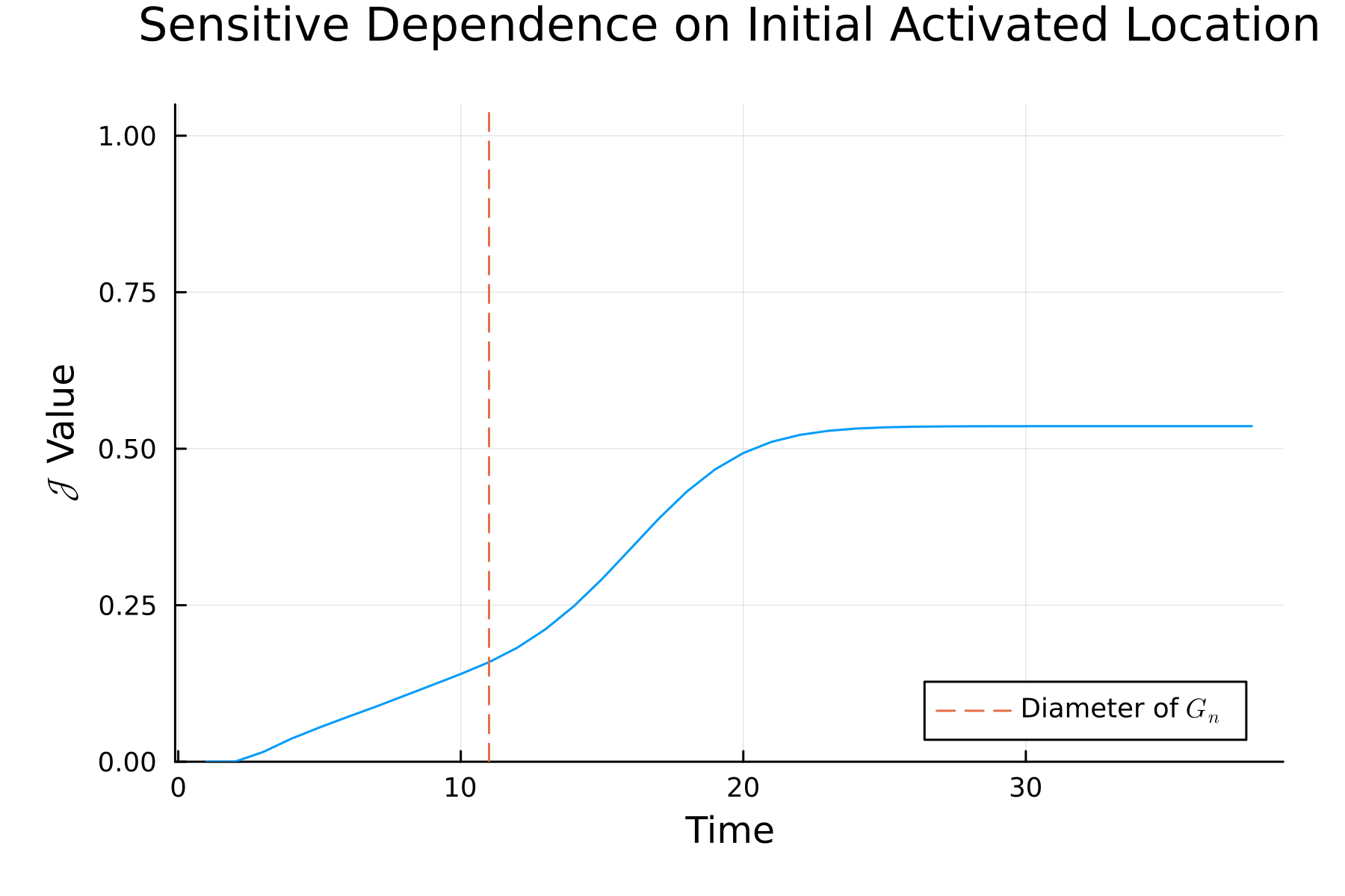
(b) $q=4$

(c) $q=2$

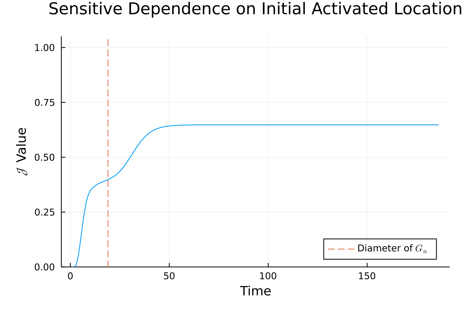
(d) $q=2$

Figure 3. Panels 3(a) and 3(c) show simulations of Theorem 1, while Panels 3(b) and 3(d) show simulations of Theorem 2. In Panels 3(a) and 3(c), we simulate 2,500 iterations of the diffusion process on both $L_{n}$ and $G_{n}$ for each value of $q$, re-drawing $E_{n}$ for each simulation. We then track the expected number of ever-activated nodes under each simulation at each time period, and then take the ratio. In order to understand how this empirical result compares to the asymptotic regimes studied theoretically, we plot the diameters of both $L_{n}$ and the average $G_{n}$. The ratio of expected activations declines monotonically until the diffusion process reaches the “edge" of $G_{n}$. Panels 3(b) and 3(d) each fix a separate draw of $E_{n}$, then each choose a fixed $j_{0}$. We then simulate 2,500 diffusion processes while tracking the Jaccard index after perturbing the initial seed location. Alternate initial location $j_{0}$ is chosen nearby to $i_{0}$, in accordance with Theorem 2. Consistent with the theoretical results, ${\mathcal{J}}$ begins and stays low until the diffusions saturate the graph, meaning that despite the starting points being nearby the diffusions mostly do not overlap.

In Figures 3(a) and 3(c), we plot the simulated values of $\frac{\hat{Y}_{T}(L_{n})}{\hat{Y}_{T}(G_{n})}$ over time for each graph. For $q=4$, the minimum ratio is attained at $T=13$ with a value of $0.780$, meaning the policymaker would underestimate the extent of the diffusion by 22 percentage points. Once the diffusion on $G_{n}$ reaches the diameter of the graph, the ratio increases towards a value just below one. For $q=2$, the minimum ratio is attained at $T=28$, taking a value of $0.169$. With a lower-dimension diffusion process, the simulations are much more sensitive to additional links in $E_{n}$. In the Appendix B.6, we show that with $q=2$ and $\beta_{n}=\frac{1}{100n}$, the minimum ratio of $\frac{\hat{Y}_{T}(L_{n})}{\hat{Y}_{T}(G_{n})}$ is still much smaller than the values attained with $q=4$. The shape of the curves in Figure 3(a) and 3(c) are similar to our theoretical results, since our results focus on asymptotic results where the diffusion cannot reach the edge of the network. Hence, the ratio in our theoretical results will continue to decline. Appendix Figure B.1 shows exactly this phenomenon by separating the ratio into separate curves for $\hat{Y}_{T}(L_{n})$ and $\hat{Y}_{T}(G_{n})$ – the separation between the two curves is maximized just after the diameter of $G_{n}$ is reached. Consequentially, the decline in the period prior to reaching the diameter of $G_{n}$ lines up exactly with the results anticipated by Theorem 1.

Next, we investigate Theorem 2 in simulation by looking at a perturbation of an initial seed within a local ball covering 1-5% of the overall number of nodes. We fix $L_{n}$ and a particular instance of $E_{n}$ to form $G_{n}$, and set $i_{0}$ as the center of the lattice. Then, we construct $J_{i_{0}}$, the set of possible alternate seeds, and choose a $j_{0}\in J_{i_{0}}$ uniformly at random. To construct $J_{i_{0}}$, we first find the depth of the second closest links in $E_{n}$ to $i_{0}$ – call this distance $d_{e_{2}}$. Then, nodes are included in $J_{i_{0}}$ if they are at distance $d_{e_{2}}+1$ from $i_{0}$. Empirically, for $q=4$, $d_{e_{2}}=2$ meaning that the distance from $i_{0}$ to $j_{0}$ is 3. The local neighborhood around $i_{0}$, $U_{i_{0}}$ (which contains all nodes at or within distance $d_{e_{2}}+1$) of this size makes up 5.3 percent of the total nodes in the graph, while $J_{i_{0}}$ makes up 64.6 percent of the local neighborhood. For $q=2$, the distance from $i_{0}$ to $j_{0}$ is 4, while the local neighborhood of this size makes up 1.05 percent of the graph and the set of $j_{0}$ make up 31.0 percent of the local neighborhood.

To approximate $\Delta_{n}(i_{0},j_{0})$, we fix the underlying percolation as in our theory and examine the set of ever-activated nodes infected by an epidemic that begins from $i_{0}$ and $j_{0}$. We exploit the connection between percolations and the one-period SIR process, predetermining which links in the network will transmit. However, we do not condition on the event that there is some overlap between the diffusions (in Theorem 2, this is encoded in the object $\Gamma_{n}$ and is assumed). Therefore, when considering $\Delta_{n}$, the denominator can be equal to zero and thus the quantity may not be well defined. To avoid this denominator issue, we instead consider the following measure. Recall that $I_{p}(i,T)$ is the set of ever-infected nodes from a diffusion started at node $i$ at time $T$. Then we define:

$${\mathcal{J}}(T)\coloneqq{\mathbb{E}}_{P_{n}(G_{n})}\left[\frac{|I_{P}(i_{0},T)\cap I_{p}(j_{0},T)|}{|I_{P}(i_{0})\cup I_{p}(j_{0})|}\right]$$

Note that this re-arranges terms from $\Delta_{n}$ – the key difference is that when $\Delta_{n}$ is closer to 1, ${\mathcal{J}}$ quantity will be close to 0. However, both measure the notion of overlap between diffusions. Note that here, we take expectations only over the percolation on $G_{n}$, meaning we generate a single draw of $E_{n}$ and then hold it fixed. We simulate the process 2,500 times, and then take the average over simulations at each time period to get ${\mathcal{J}}(T)$. Results are shown in Figures 3(b) and 3(d).

Figures 3(b) and 3(d) indicate that there is generally little overlap between the diffusions until the process has reached the diameter of the graph and saturated the network. Recall that when ${\mathcal{J}}(T)$ is close to zero, this implies that the share of nodes that would be activated by both starting conditions as a share of the total activations is small. Hence, this implies that the activation paths are following very different portions of the network. This lack of overlap is despite the fact that $i_{0}$ and $j_{0}$ are extremely local. For $q=4$, at $T=5$ (the halfway point to the diameter of $G_{n}$), the value of ${\mathcal{J}}=0.055$ indicates almost entirely distinct processes. For $q=2$, at $T=9$ (again half of the diameter of $G_{n}$), the value of ${\mathcal{J}}=0.32$. These results are consistent with the theoretical results: there exist time periods early on in which the diffusions are almost entirely disjoint. Empirically, these results demonstrate that the diffusions remain disjoint for a relatively long period of time.

While it is clear that our simulations are highly sensitive to measurement error, regardless of whether $q=2$ or $q=4$, the changes in sensitivity are instructive. Comparing $q=2$ to $q=4$, the simulations demonstrate that the diffusion process is much more sensitive in terms of the extent of diffusion with lower dimension, rather than the location. This is because $q=2$ ensures that a greater fraction of connections are “local” – therefore, there can be less local perturbation. However, i.i.d. connections lead to many more activations. Nonetheless, we note that there is still severe sensitive dependence on initial conditions with $q=2$ – in the short run only a third of the diffusion overlaps on average.

6.2. Aggregate Patterns Are Well-Approximated by Compartmental Models

Next, we study the approximation of the diffusion process by a standard differential equations SIR compartmental model. In practice, diffusion occurs between a discrete set of $n$ agents and transmission occurs over discrete time. The compartmental differential equations model simplifies matters by using a mean field approximation, but there is a potential for error which we now explore.

We assume that the econometrician fits the following model to data which is generated by a diffusion on $G_{n}$. Let $S(t)$, $I(t)$, and $R(t)$ be the susceptible, infected, and removed nodes at time $t$. Then the change in each quantity at time $t$ will be given by:

$$\dot{S}(t) :=-\frac{s}{n}S(t-1)I(t-1)$$

$$\dot{I}(t) :=\frac{s}{n}S(t-1)I(t-1)-rI(t-1)$$

$$\dot{R}(t) :=rI(t-1),$$

where $s$ and $r$ are parameters to be estimated using the diffusion data through some time period $\hat{t}$. Note that ${\mathcal{R}}_{0}=s/r$.

We conduct two exercises. In the first exercise, we simulate a diffusion process on $G_{n}$ for $T$ periods. We then estimate the parameters of interest, ($\hat{r},\hat{s})$ at $\hat{t}=T/4$ and we generate forecasts from the compartmental model. We compare this to the actual diffusion trajectory. The second exercise replicates the first, with the only change being that we simulate the diffusion process on $L_{n}$ instead. Note that this is not what generates the diffusion process in the “real world”—that is diffusion on $G_{n}$. However, together the two simulations capture two features: (a) the deviation of the mean-field model from the underlying discrete process and (b) how the deviation depends on the relative structure of $G_{n}$ to $L_{n}=G_{n}-E_{n}$. We repeat both sets of simulations for both $q=4$ and $q=2$.

In practice, we run a number of simulations in each configuration. We then fit $(\hat{r},\hat{s})$ for each simulation draw and then average them to produce forecasts which then can be compared to $\hat{Y}_{T}(L_{n})$ and $\hat{Y}_{T}(G_{n})$ (both of course averaged over simulation draws) which we then print below. Details are given in Appendix B.5.

Figure 4 presents the results. We begin with $q=4$ and it is helpful to look to the diffusion on $L_{n}$ first in Panel 4(a). Recall that this shows how well the mean-field approach captures the dynamics on a hypothetical network structure ignoring links in $E_{n}$. In the periods where the SIR process is fit to the simulated data, the fit is very good. The estimated $\hat{\mathcal{R}}_{0}$, derived by taking the average across simulations of $\hat{s}/\hat{r}$, is 1.46 under $\hat{Y}_{T}(L_{n})$, well below the true ${\mathcal{R}}_{0}$ of 2.5. Note that while Lemma 1 implies that there exists a consistent estimator of ${\mathcal{R}}_{0}$, the estimator we propose in theory uses activation-level data. Here, we base our estimate of $\hat{\mathcal{R}}_{0}$ using the aggregate diffusion pattern. The estimated forecasts (in orange) diverge quickly from the true diffusion, $\hat{Y}(L_{n})$. Because of the initially exponential growth structure of the compartmental model, early in the medium run it overshoots, though the diffusion saturates much earlier and in fact the overall diffusion count in the long run is underestimated.

That is, in sample, the compartmental model can be made to fit well, but with a lower growth rate for the number of ever-infected nodes. However, because of the lower implied ${\mathcal{R}}_{0}$, the compartmental model dramatically underestimates the total number of expected activations out of sample. Ex-post, a policymaker could fit this type of model and do extremely well, but it would not be helpful for predicting the future trajectory.

In Panel 4(b), we turn to diffusion on $G_{n}$. The estimated $\hat{\mathcal{R}}_{0}$, derived by taking the average across simulations of $\hat{s}/\hat{r}$, is 1.52 under $\hat{Y}_{T}(G_{n})$, still below the true ${\mathcal{R}}_{0}$ of 2.5. We find very similar results as the case with $L_{n}$. The principle difference is that the idiosyncratic links, $E_{n}$, generate a slightly closer forecast curve to the true trajectory. Also of note, the implied diffusions from the compartmental model on $L_{n}$ and $G_{n}$ are also similar. While the estimates are such that the historical fit is quite good, the exponential structure makes the process run too fast and then fade too early as well, relative to a slower more persistent polynomial process (which of course could be historically fit by looking backwards).

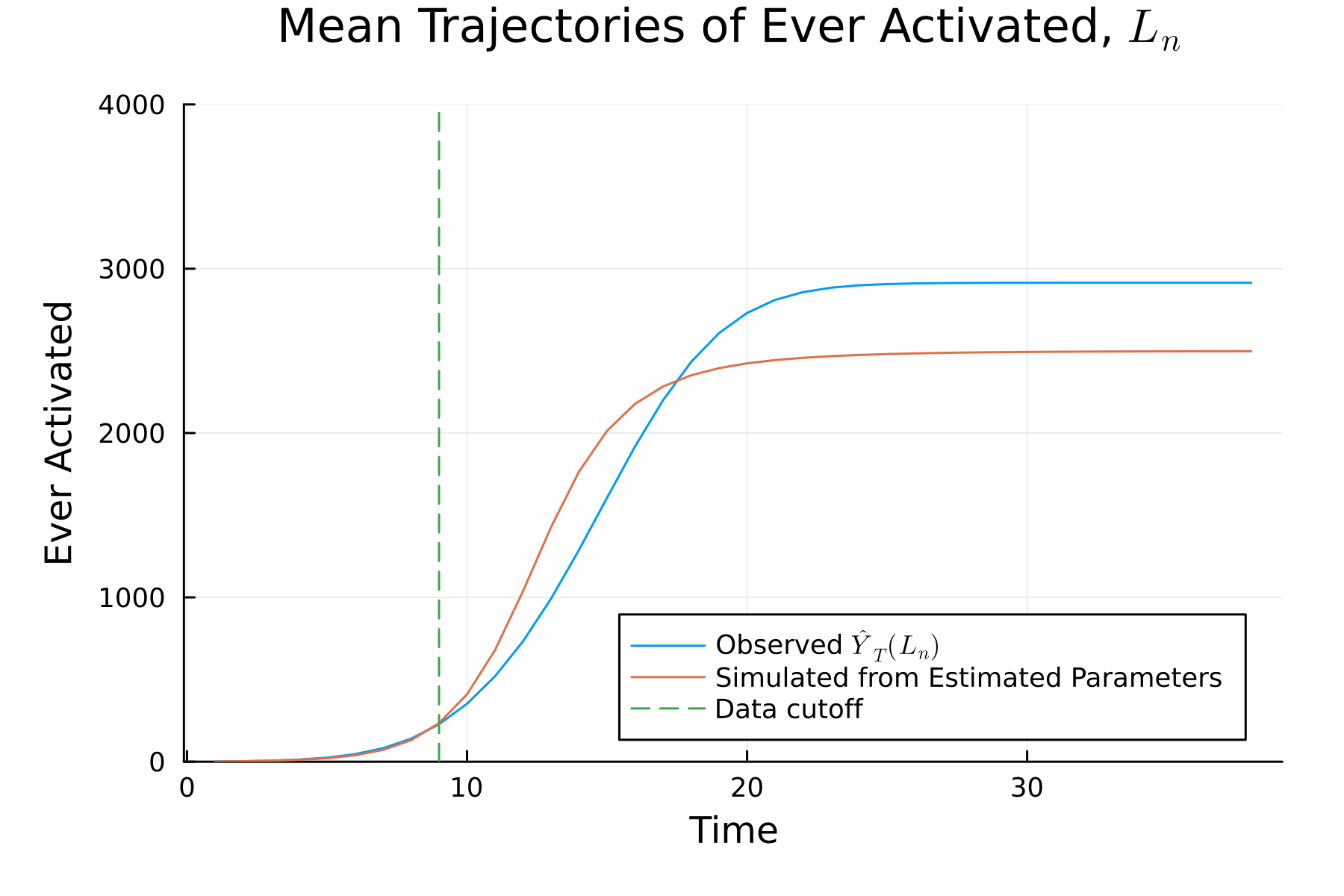
(a) $q=4$

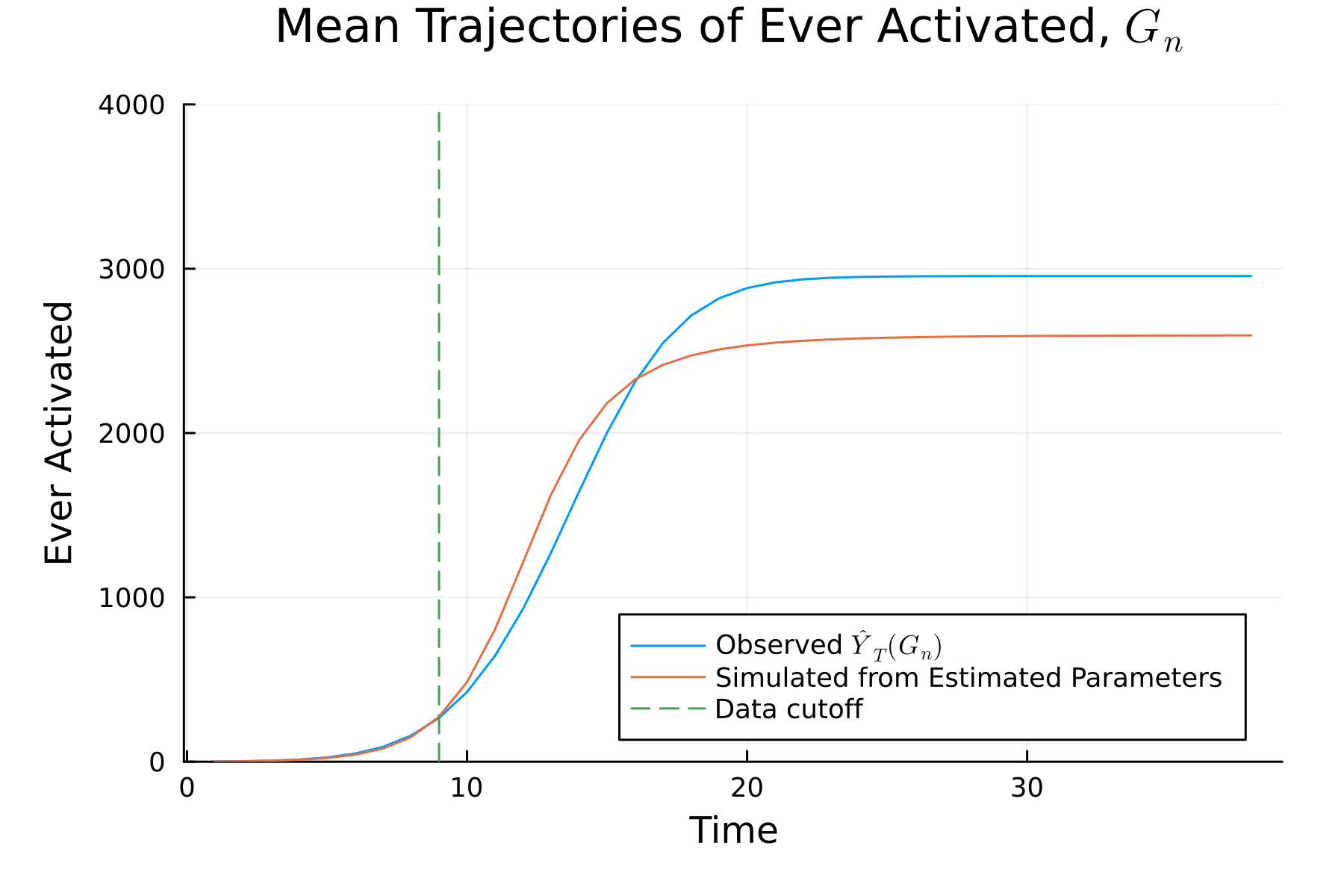
(b) $q=4$

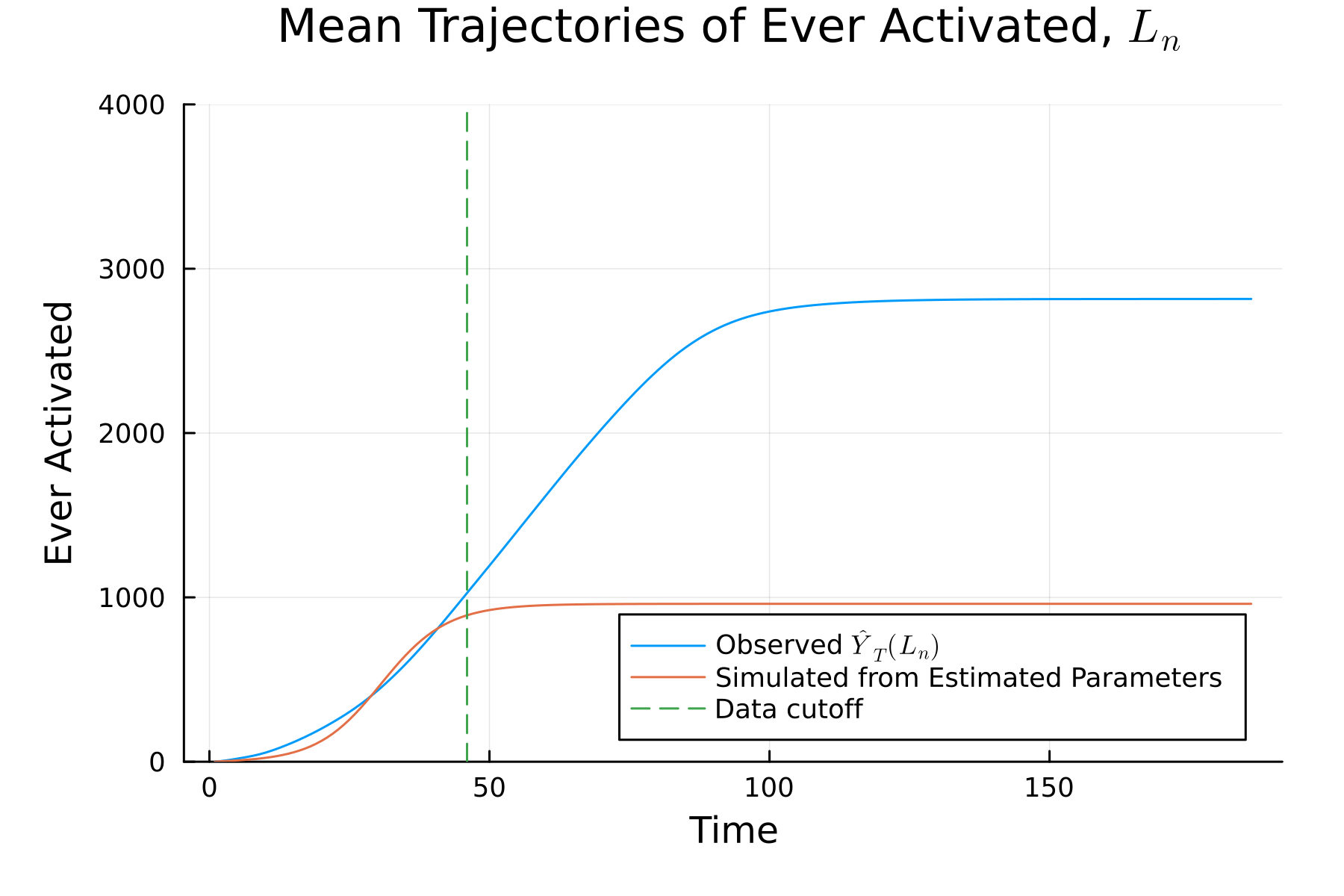
(c) $q=2$

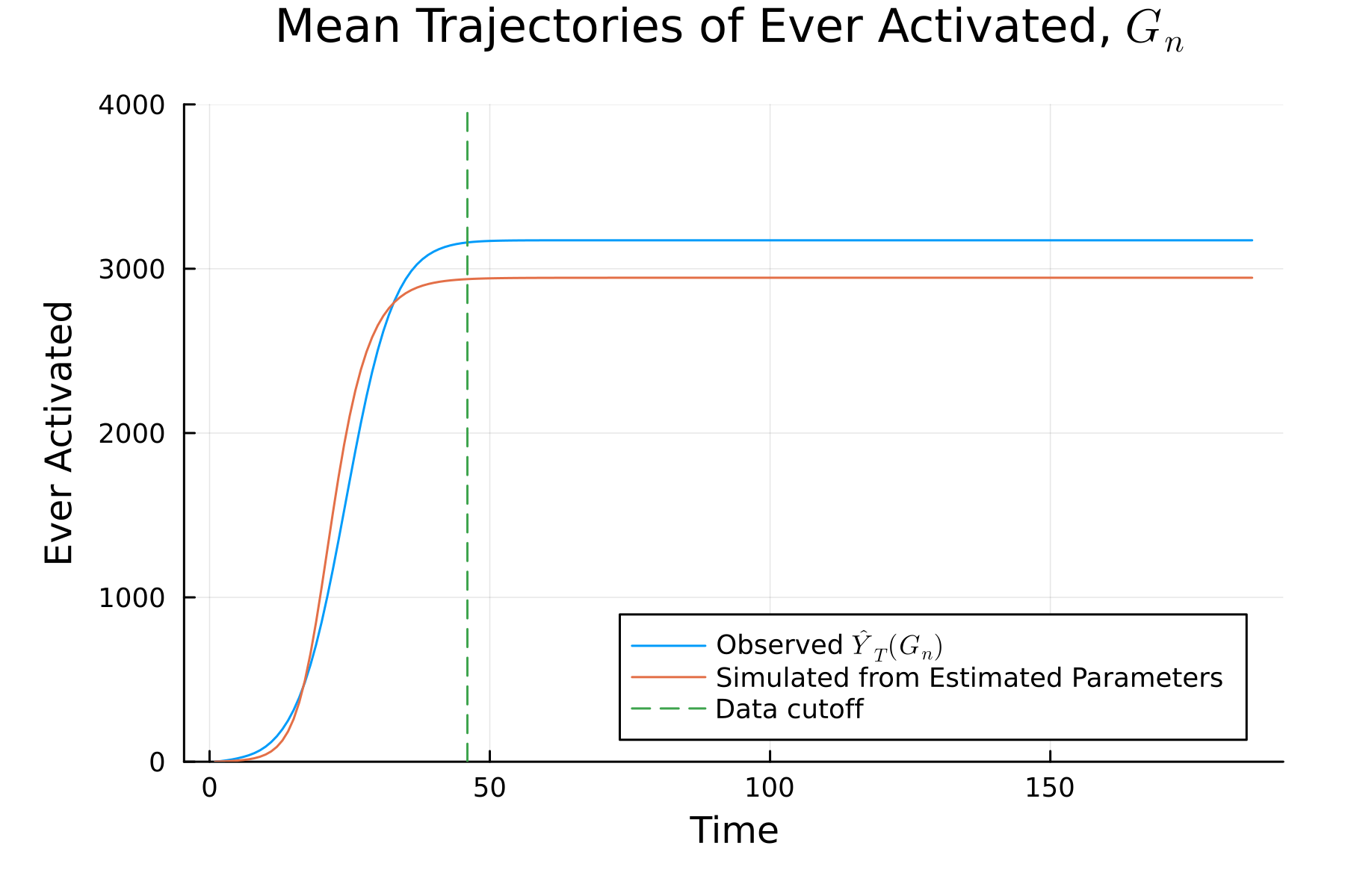
(d) $q=2$

Figure 4. A comparison of the mean ever activated under the true network SIR model and the estimated trajectory from the differential equations model. Panel (A) and (B) use $q=4$, while (C) and (D) use $q=2$. Panel (A) shows simulations when $\hat{Y}_{T}(L_{n})$ is used as the data generating process, while Panel (B) shows when $\hat{Y}_{T}(G_{n})$ is used. The data cutoff is at $T/4$. Before this point, the compartmental SIR model is fit to the data via the generalized method of moments. After this point, we run the differential equation model forward to see how it performs out of sample.

For $q=2$, there is a shift between $L_{n}$ and $G_{n}$. With $q=2$ and $L_{n}$, as seen in Panel 4(c), the process cannot be well approximated by the model. The fitted compartmental SIR looks almost nothing like the true trajectory: while fitting to data the SIR model makes a complete “S” curve shape, it dramatically underestimates the total activations. Turning to the $G_{n}$ case, as seen in Panel 4(d), the compartmental SIR model is able to match the data more closely, because the diffusion moves much more quickly.

In sum, a compartmental SIR model can, in many cases, be fit well looking backwards to a polynomial diffusion process. This fit is even better the higher the dimension of $L_{n}$, as it admits more expansive balls. But in all cases, the compartmental SIR estimates to rapid a diffusion that saturates and then stabilizes too quickly: historical aggregate fits may be excellent and at the same time they may serve as poor forecast tools.

7. Empirical Applications

We now consider three empirical applications. The first examines the COVID-19 pandemic, which showcases our results in a large scale setting. In addition, it demonstrates how only local linking can still cause errors in diffusion – though we show that the problems are much worse in the idiosyncratic case. The second example studies mobile phone marketing in India, which showcases our results in a much smaller scale setting. Here, sensitive dependence on initial location has much more dramatic results – volumes of diffusion are more robust in this setting, because the networks themselves are much smaller. Finally, we consider the diffusion of a weather insurance product in China. Here, we consider how errors in a diffusion model could impact statistical power when estimating peer effects.

7.1. Data from the COVID-19 Pandemic

Kang et al., (2020) introduces a dynamic human mobility flow data set across the United States, with data starting from January 1st, 2019. By analyzing millions of anonymous mobile phone users’ movements to various places, the daily and weekly dynamic origin-to-destination population flows are computed at three geographic scales: census tract, county, and state. We study tract-to-tract flows on March 1st, 2020, at the start of the COVID-19 pandemic in the United States. Note that this date was before the WHO declared COVID-19 a pandemic and before the United States declared a national state of emergency. For the sake of computational tractability, we focus on a region in the Southwest of the United States that contains all of California and Nevada, along with a small portion of Arizona. A map of the region is shown in Appendix Figure C.1.

We use this real-world dataset to simulate disease transmission as in Section 6.1. One approach would be to construct a network with unweighted edges between two census tracts if at least one person moves between them. However, this results in an extremely dense graph. The resulting graph has a diameter of $4$, a mean degree of $143.82$, and a max degree of $991$. The density of the network will result in the epidemic spreading everywhere in a very short period of time, negating the need for forecasting.

Realistically, researchers may decide to “prune” the network by only including links where there is sufficient traffic between two census tracts. In this case, a missing link implies a (potentially large) flow of people between two places, rather than missing a single individual contact. Hence, we construct the observed $L_{n}$ by linking tracts if the average flow between them (averaging over directions) is greater than six trips (the 93rd percentile of all flows). We then consider two ways to define the “true” base graph $G_{n}$. The first, denoted $G_{n}^{92}$ links tracts if the average flow exceeds five trips (the 92nd percentile), meaning that $E_{n}^{92}$ includes links of exactly 6 trips. Further discussion of the pruning procedure is given in Appendix C. The other, $G_{n}^{\beta}$, adds links i.i.d. with probability $\beta_{n}=\frac{1}{0.32n}$ corresponding exactly to the extra links missed going from the 5 trips to 6 trips, with these links now placed idiosyncratically. Properties of the resulting $L_{n}$ and $G_{n}$ are shown in Table C.1.

We begin by simulating Theorem 1 and calculating the share of $Y_{t}(L_{n})/Y_{t}(G_{n})$ for our two $G_{n}$ measures. In the first, we look at $G_{n}^{93}=L_{n}$, where $L_{n}$ amounts to pruning about 18 percent from the $G_{n}^{92}$ graph. Here, because $G_{n}^{92}$ is a (non-stochastic) function of the data, we hold it fixed and take expectations only over the path of the epidemic. In the second, we generate $G_{n}^{\beta}$ via $L_{n}\cup E_{n}$, where $E_{n}$ has i.i.d. links to generate the same density as the error graph in the pruning procedure. As before, in both cases, we choose $i_{0}$ uniformly at random and hold it fixed across simulated epidemics.

We plot $Y_{t}(L_{n})/Y_{t}(G_{n})$ over time in Figures 5(a) and 5(c). For $G_{n}^{92}$, the pruned network, the minimum ratio of $0.442$ is achieved at $T=8$. We note that this ratio has the same qualitative pattern as in the simulated graph in Section 6.1 – the ratio achieves a minimum just before reaching the diameter of $G_{n}^{92}$, and then slowly increases. When compared to the previous simulations, the ratio increases much more slowly. This result comes from the larger dispersion in degrees – it takes longer for the disease to fully saturate the network, because there are more nodes with very few links. When compared to the i.i.d. errors in $G_{n}^{\beta}$, the minimum ratio of $0.234$ is achieved at $T=9$. One explanation for i.i.d. errors leading to additional underestimation follows from Theorem 4. The pruning procedure induces spatially clustered errors – so for the same level of error, the spatially clustered additional links in $G_{n}^{92}$ will not jump as far as $G_{n}^{\beta}$, leading to fewer “new” shells of infection.

Next, we simulate a version of Theorem 2. We follow a similar procedure as with Section 6.1, tracking ${\mathcal{J}}(T)$. We choose $j_{0}$ in a conservative fashion – after fixing a $i_{0}$ uniformly at random, we choose the set of potential $j_{0}$, $J_{i_{0}}$, to be all nodes at distance two from $i_{0}$. In $G_{n}^{92}$, the local neighborhood containing all potential $j_{0}$, $U_{i_{0}}$, makes up 1.57 percent of the graph, while the set of $J_{i_{0}}$ makes up 81.68 percent of the local neighborhood. In $G_{n}^{\beta}$, $U_{i_{0}}$ contains all $j_{0}$ comprises 2.93 percent of the graph, and $J_{i_{0}}$ makes up 93.46 percent of $U_{i_{0}}$.

We plot ${\mathcal{J}}(t)$, the amount of overlap between percolations over time, in Figures 5(b) and 5(d). These results follow the same qualitative pattern as before – ${\mathcal{J}}(t)$ stays close to zero for the first few time steps while the epidemics are almost entirely distinct, but then slowly increases. For the first few time periods, this graph shows dramatic sensitive dependence on the initial starting point of the epidemic. For the pruning procedure, halfway to the diameter of $G_{n}^{92}$, ${\mathcal{J}}=0.42$. For the i.i.d. procedure, halfway to the diameter of $G_{n}^{\beta}$, ${\mathcal{J}}=0.023$.

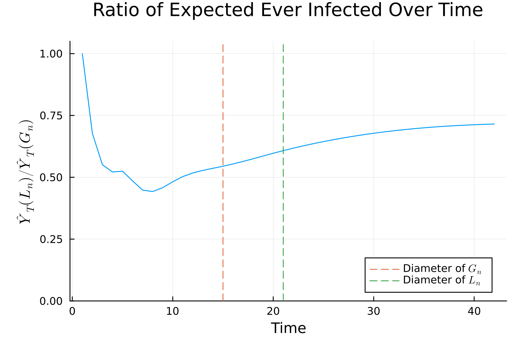
(a) Pruning

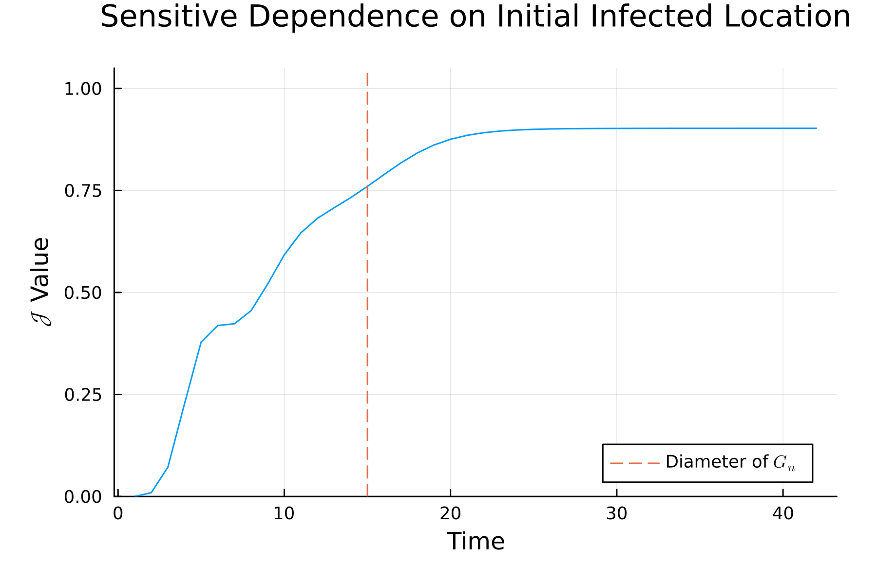
(b) Pruning

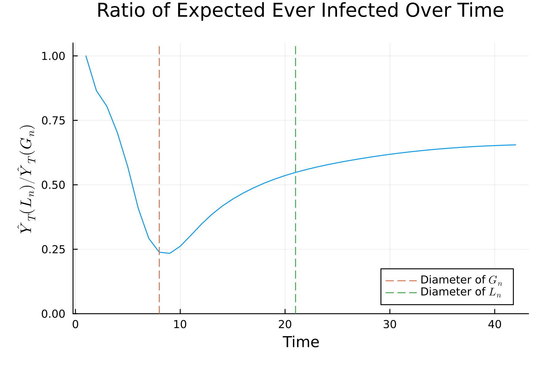
(c) I.I.D.

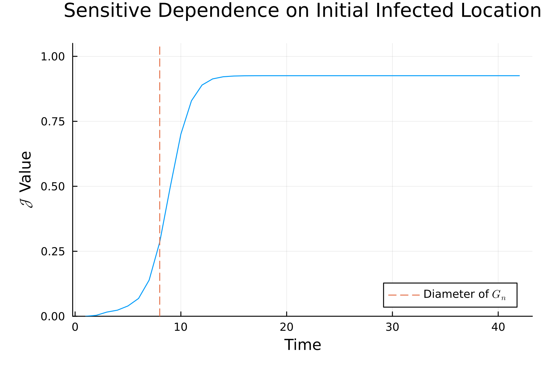
(d) I.I.D.

Figure 5. Simulated version of Theorems 1 and 2 on $L_{n}$ and $G_{n}$ generated from Census tract flow data in California and Nevada. Panels (A) and (C) show simulations of Theorem 1, while Panels (B) and (D) show simulations of Theorem 2.

7.2. Diffusion in Mobile Phone Marketing

As a second empirical exercise, we study the diffusion of high-value information in Indian villages. The goal of this exercise is to highlight how the measurement issues can crop up in settings with much smaller networks, and how the initial seed condition plays a much larger role here. In Banerjee et al., (2019), one of this article’s authors, along with collaborators, conducted a randomized controlled trial wherein randomly selected people in villages in Karnataka were given information on a program where they could receive a high-value cell phone or smaller cash prizes if they participated. The information about the program then diffused throughout the village.

We use this data to study the robustness of the diffusion process in an information setting, using the subset of villages for which network data was collected. Average village-level network statistics are shown in Table D.1. Details on how the graphs are constructed are in Appendix D. In a change from the prior simulations and analysis, many of the villages have multiple initial seeds. There are on average 3.26 seeds per village, and on average there are 196 nodes per village.

We first estimate the passing probability $p_{n}$ for the diffusion process. Villagers could indicate they heard about the cell phone program by making a free call to the researchers. While we observe data on the sampled networks connecting households, we only observe the total number of calls received by the researchers in each village, and we do not observe whether a given household made a call. Hence, we back out the passing probability $\hat{p}_{n}$ using the method of simulated moments. Formally, we consider the following problem. Let $V=69$ be the number of villages in our data (for which we have network data) and let $C_{v}$ be the number of calls received in village $v$. We treat the number of calls as the number of ever-activated nodes. We then simulate a SIR process with passing probability $p$ and record the number of simulated calls after $T$ periods. Let $\hat{C}_{v}^{s}(p)$ be the simulated number of calls in simulation $s$ under passing probability $p$. Then, we choose $\hat{p}_{n}$ as follows:

$$\hat{p}_{n}=\text{argmin}_{p}\left(\frac{1}{V}\sum_{v=1}^{69}\left(C_{v}-\frac{1}{s}\sum_{s}C_{v}^{s}(p)\right)\right)\left(\frac{1}{V}\sum_{v=1}^{69}\left(C_{v}-\frac{1}{s}\sum_{s}C_{v}^{s}(p)\right)\right)$$

We set $T=15$, just larger than twice the average diameter of a village graph and use 2,500 simulation iterations. We estimate a value of $\hat{p}_{n}=0.13$, meaning that each household transmits the information with roughly one in six chance. We then use this estimated $\hat{p}_{n}$ to conduct simulations.

Next, we consider the error structure $E_{n}$ on our observed network $L_{n}$. Since our data has many separate villages, we consider a slightly more complex structure for $E_{n}$. Let $n_{v}$ be the number of households in village $v$. Then, we form $E_{n}$ by taking the union over draws of Erdos-Renyi random graphs in each village, where $\beta_{n}^{v}=\frac{1}{2n_{v}}$ changes in each village to keep measurement error proportional to village size. We choose a proportionally larger value of $\beta_{n}$ because there are multiple seeds – because the graph becomes saturated much more quickly, measurement error has less time to become a problem.

We first simulate a version of Theorem 1. We simulate 2,500 diffusion processes across each village, adding up the total number of households who ever get the information and averaging across simulations. We run this simulation both on $L_{n}$, the set of village graphs, and $G_{n}$ constructed as above (with a new draw of $G_{n}$ in each simulation iteration). As shown in Figure 6(a), the ratio $\hat{Y}_{T}(L_{n})/\hat{Y}_{T}(G_{n})$ monotonically decreases over time, taking value $0.854$ at $T=15$. Despite the village-level networks being relatively small, in aggregate, the econometrician still underestimates the extent of diffusion by nearly 15 percentage points.

To simulate a version of Theorem 2, we choose a modified seed set for each village. Recall that most villages have multiple seeds. Here, we perturb the seed set in each village in a conservative manner. Say that a seed set is comprised of $\{i_{0},j_{0},k_{0}\}$ in some village. We choose one element of the seed set at random, say $k_{0}$, and then replace $k_{0}$ in the seed set with a neighbor chosen uniformly at random. This corresponds to a local neighborhood of 3.5% of the entire network on average. Despite the conservative perturbation, we still find similar results, as shown in Figure 6(b). As before, we track ${\mathcal{J}}(t)$, the Jaccard index for the aggregate patterns of diffusion across all villages over time. While the value of ${\mathcal{J}}(t)$ does not start at 0 (as in the prior simulations), given the multiple seeds and that we conservatively only perturb one, it remains below 0.75, indicating that despite the conservative perturbation, there is still not complete overlap in the perturbed diffusion processes. Halfway to the diameter of $G_{n}$, the average value of ${\mathcal{J}}=0.61$ indicates a lack of overlap.

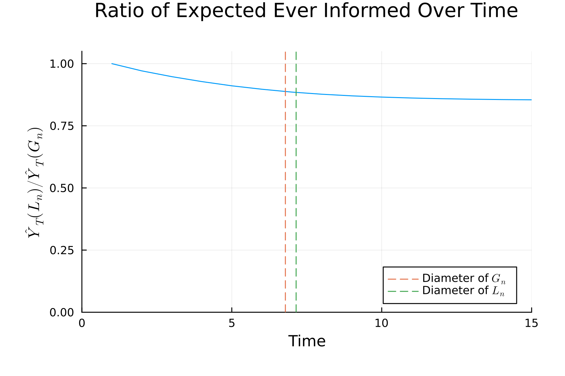
(a)

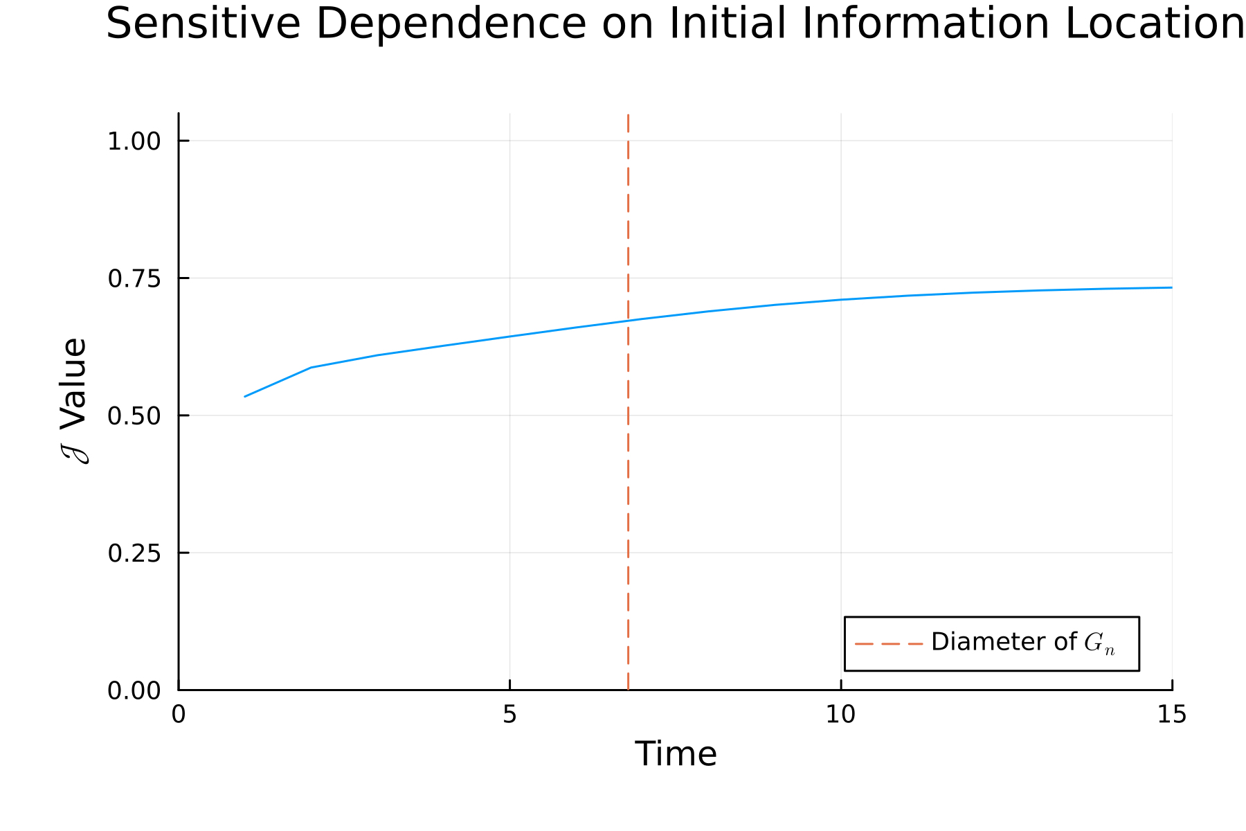
(b)

Figure 6. Simulations of Theorems 1 and 2 on village networks from Karnataka, India. Panel (A) shows a version of Theorem 1. We take 2,500 diffusion simulations on $L_{n}$ and $G_{n}$, where $G_{n}$ is constructed at the village level with $\beta_{n}=\frac{1}{2n_{v}}$. $n_{v}$ is the number of households in the village. Panel (B) shows a version of Theorem 2. We perturb one seed uniformly at random by a single set in each village. Then, we simulate 2,500 diffusion processes on a fixed draw of $G_{n}$, computing the average Jaccard index of the process.

7.3. Treatment Effects with Spillovers in Networks

As a third empirical exercise, we study the uptake of insurance in rural China. The goal of this exercise is to illustrate how the problems we identify in diffusion could affect conclusions from an estimated model of peer effects. If nodes are seeded with information, then the take-up behavior of a product may be a function of “exposure to information” through the diffusion process. A typical peer effects regression would consider the outcome regressed on this exposure to treatment as defined through a diffusion model; our analysis suggests that results could be biased and estimators could lose considerable power.

In Cai et al., (2015), they give farmers information about a weather insurance product, a product with low adoption rates that is highly valuable. Intensive information sessions were randomly given to some farmers. The authors then measure the take-up by other people in the same village, who were not part of the first set of information sessions. We consider a measure of exposure to treatment based on a model of information flows.

We first take the data from Cai et al., (2015) and build the village networks. We convert the directed networks from the paper to undirected networks, where household $i$ is linked to household $j$ in our construction of the data either if $i$ reports $j$ as a link, $j$ reports $i$ as a link, or both. The resulting graph is denoted $G_{n,v}$ for village $v$. Graph statistics for the villages are shown in Table E.1.

We consider an exposure measure based on a model of information flows. For a generic graph, let $A$ be the corresponding adjacency matrix. Let $s$ be a vector of indicators, with an entry equal to one if the household attended an information session. For a given $p_{n}$ and $T$, we define the vector of “diffusion exposure” as,

$$DE^{A}=\left(\sum_{t=1}^{T}(p_{n}A)^{t}\right)s,$$

which calculates the expected number of times that each individual hears information through repeated passing over $T$ periods (Banerjee et al.,, 2019). We imagine that the take-up of insurance in Cai et al., (2015) increases in such exposure to treatment: hearing more about the product through conversation makes one more likely to take up. Note that this exposure measure, based on how often a person hears about the product, is slightly different than a typical SIR model. It considers the eventual outcome as depending on the total number of times person $i$ hears about the topic through $T$ periods, rather than a once-and-for-all decision the first time someone hears about the product. This model is perhaps a more realistic description of the take-up of an insurance product. Nonetheless, the mechanics of error we outline in the paper have analogs for this kind of model.

We then simulate an experiment. We treat the data from Cai et al., (2015) as the true network $G_{n}$. We then regress insurance take-up ($y_{i,v}$) on the exposure measure ($DE_{i,v}^{G}$), a set of household controls ($X_{i,v}$), and village fixed effects ($\mu_{v}$),

$$y_{i,v}=\alpha+\gamma DE_{i,v}^{G}+X_{i^{\prime}v}^{\prime}\delta+\mu_{v}+\epsilon_{i,v},$$

where $i$ indexes household and $v$ indexes village. To do so, we subset the data to only households who did not receive the initial informational intervention. We standardize the exposure measure to have mean zero and standard deviation one for the sake of interpretability. Results are shown in Table 1. We document that a one standard deviation increase in diffusion exposure increases insurance uptake by 2.9 percentage points (s.e. 1.2 percentage points, $p=0.02$), relative to a mean of 45.9%, in a linear probability model.

	Insurance Uptake
Diffusion Exposure	0.029
	(0.012)
Household Controls	Yes
Village FE	Yes
Num Obs.	2676
Uptake Mean	0.459

Table 1. A regression of diffusion exposure on insurance uptake, with diffusion exposure computed from the networks collected in Cai et al., (2015). Standard errors are clustered at the village level. Household controls include household head age, education, and gender, along with rice area farmed, income from rice farming, and household degree.

We then drop links in $G_{n}$ with i.i.d. probability $\beta_{n}$ and construct the observed network $L_{n}$. That is, we imagine that there is a small measurement error in our survey process (or network construction process) and for this exercise we allow the error to be fully i.i.d. Errors may be correlated with factors such as geography, place of work, etc., which may be emphasized or used in constructing network data. Our simulation corresponds to what the researcher would have observed had information flowed over $G_{n}$, but they instead measured $L_{n}$.

For each village $v$, we drop links with probability $\beta_{v,n}$, operationalized by intersecting the corresponding village graph with an Erdos-Renyi random graph with links that form with probability $1-\beta_{n}$. We vary the value of $\beta_{v,n}=\frac{1}{k\bar{d}_{v}}$, where $\bar{d}_{v}$ is the village average degree and $k$ is a specified constant. We vary $k$ from 5 to 15 or $\beta_{v,n}$ ranging from 0.037 to 0.0123. We then recompute the diffusion exposure ($DE^{L}_{i,v}$), re-estimate the regression, and record the point estimate and $p$-value on diffusion exposure. We repeat this process 2,500 times for each value of $k$. Let $\hat{\gamma}(G_{n})$ and $\hat{\gamma}(L_{n})$ be the coefficients of interest from the two regressions.

Figure 7 plots the joint distribution of the bias percentage—the percentage difference between $\hat{\gamma}(L_{n})$ and $\hat{\gamma}(G_{n})$—and the rejection level (one-to-one with the $p$-value) of the null of the coefficient $\hat{\gamma}(L_{n})$ being equal to zero. While on average the bias is small, for any given draw, we see large dispersion in the difference between $\gamma(G_{n})$ and $\gamma(L_{n})$ even when a very small fraction of links are dropped. This is striking. Notice that in the real world, the econometrician observes only a single draw—one instance of this phenomenon. The result shows that enormous biases are likely in any single draw. Here, even with the smallest $\beta=0.012$, we find the bias still has a large standard deviation of nearly 8 percentage points. With $\beta=0.037$, biases upwards of 20% in magnitude are common.

We also see a range of p-values: as we decrease $\beta$, we would expect to see the p-values converge to the true value. Specifically, with no noise we know $p=0.02$ and so for very small $\beta$ we might imagine that we reject the null of no peer effect at the 95% level ($0.02<0.05$). However, with $\beta=0.037$, we fail to reject (at the 95% level) the null of no peer effects over 15% of the time. And in the even more extreme case of $\beta=0.012$, we still fail to reject the null of no peer effects 4.5 percent of the time. This means that even though with no measurement error we have $p=0.02$, with a very small error anywhere between roughly 5% to 15% of the time we may be unable to reject a null at the 95% level.

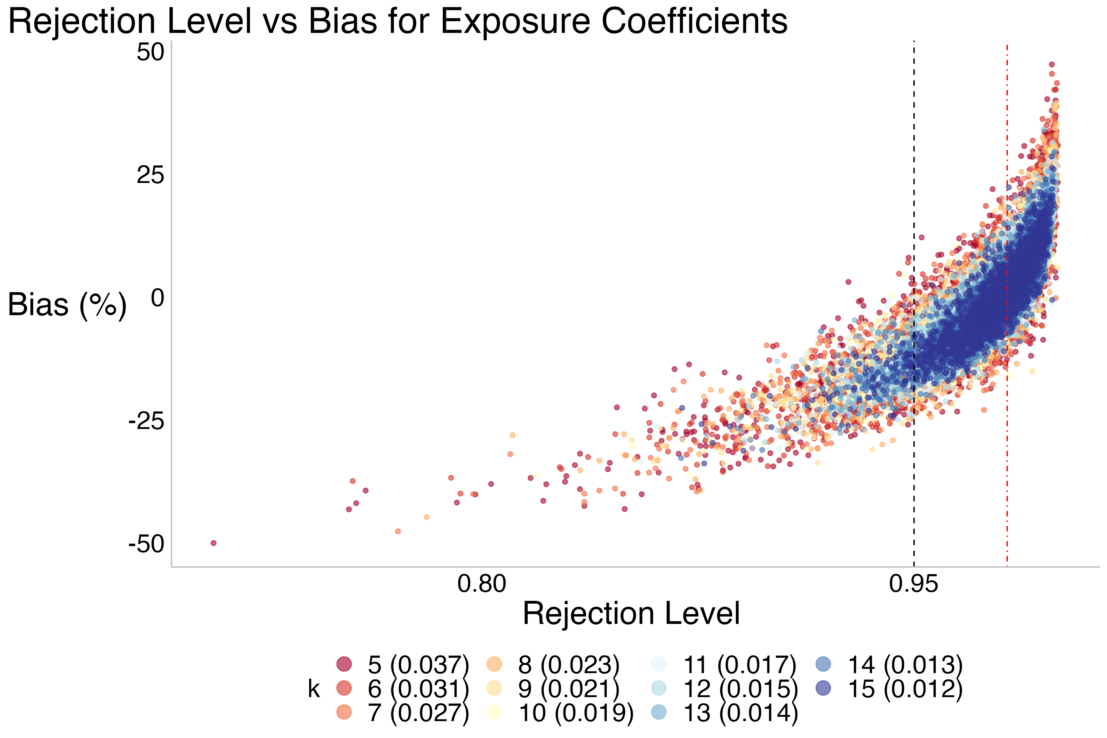
Figure 7. The joint distribution of the difference in $\hat{\gamma}(L_{n})$ and $\hat{\gamma}(G_{n})$ (in percentage terms) and the level at which we can reject the null that $\hat{\gamma}(L_{n})=0$ for different values of $k$. As $k$ increases, $\beta_{v,n}$ decreases. In parenthesis, we include the average value of the corresponding $\beta_{n}$ across villages. The red, dashed, vertical line denotes the level at which we can reject $\hat{\gamma}(G_{n})=0$, while the black dotted line shows rejection at the 95 percent level.

8. Discussion

In this paper, we have studied the lack of robustness to even small quantities of mismeasurement in SIR diffusion models on networks. Such models are widely used to conceptualize epidemics, information flow, and technology adoption, among other applications. We focus on the medium-term part of the regime when questions about forecasting the extent and location of the diffusion and identifying the space for policy interventions are relevant. For the bulk of the paper we analyze what we call polynomial diffusion over these time horizons, capturing the idea that if it were globally exponential then the diffusion would blanket the society almost immediately. These reflect real-world contagion processes where geography, homophily, transport infrastructure, and community interactions shape the diffusion.

We have seen that a number of quantities of interest to policymakers, such as diffusion forecasts, estimates of where the diffusion has occurred in the network, and the efficacy of further data collection or widespread testing may all be problematic in the face of extremely small measurement errors in the network. In many cases, network data collection is known to be imperfect, but the econometrician may have knowledge of the structure of errors. In the case where the error has a known structure, the econometrician can correct for sampling error by integrating over the error (Chandrasekhar,, 2016). However, this approach will only work in the case of exactly correct specification of the error model; any departure could potentially generate missing links, meaning our results become relevant. In the case where one knew $\beta_{n}$, one could use this strategy to integrate over $E_{n}$. However, given Theorem 2, the set of possible activated nodes in this exercise could be geographically disparate.

In fact, we have shown that even if the missed links constitute not only a vanishing share of the overall links at a very rapid rate but also are only concentrated locally to any node in question (that is, the errors occupy a vanishing neighborhood relative to any node), the problems persist. This means that the problems are not consequences of long-range shortcuts and transitioning polynomial-like diffusion to exponential-like diffusion as in the small worlds literature. Rather, the point is that even small infrequent errors that are entirely localized wind up aggregating throughout the SIR process, thereby generating all of the aforementioned problems.

Our work demonstrates the general care needed in identifying the limits of what models can reasonably predict to inform policy. Tools must be used for exactly what they are developed. Aggregate concepts geared towards retrospective calculations may be good for just that– certain aggregates, e.g., $\mathcal{R}_{0}$, may better be used as descriptive rather than prescriptive tools.

Of course, this raises practical concerns for any normative work that builds on the scaffolding of such models. Almost certainly the failure of robustness would propagate to welfare calculations, which often rely on the extent of diffusion or the locations (or composition or compartments) of diffusion, if not both (Acemoglu et al.,, 2021; Fajgelbaum et al.,, 2021). It is possible, though requires future work, that the susceptibility to small measurement error presents an argument for policymakers to respond earlier and much more aggressively. Barnett et al., (2023) make the point that in an uncertain world, policymakers may want to pursue more aggressive containment policies to guard against worst-case scenarios. The full decision theory exercise is beyond the scope of this paper, but it should be clear that this is the thrust of the statistical force given the massive uncertainty we document. In fact, we view these results as highlighting exactly how challenging it is to model dynamics on networks, rather than steady-state features of the network, analogous to many of the challenges in other economic settings.

This paper is specific to SIR models on graphs, but the phenomenon need not be. In fact, the same sort of perturbation robustness failure may impact general models of treatment effects with spillovers (e.g., Aronow and Samii, (2017) and Athey et al., (2018)). The final empirical example that we presented, using the insurance take-up data from Cai et al., (2015), suggests this is exactly the case. An examination of perturbation robustness failure in general models of treatment effects with spillovers is likely worth studying in its own right which we leave to future work.

Appendix A Proofs

Proof of Theorem 1.

Recall that

$${\mathcal{E}}_{t}={\mathbb{E}}\left|\{x\in L_{n}\mid x\textrm{ ever activated by the diffusion on }L_{n}\}\right|.$$

We can first note that the numerator is exactly:

$$\hat{Y}_{T}(L_{n})={\mathcal{E}}_{T}$$

We can then bound this quantity from above using Assumption 1. The denominator will require more work. We can start by noting that we can partition $L_{n}$ into $K$ disjoint “tiles", which generates strictly less activation than if the tiles were still connected. The tiling is a counting device – instead of counting overall activations, we count the number of tiles that are activated, and then scale those values by the number of periods for which the diffusion spreads. Each tile is composed of a subset of $L_{n}$ that is disjoint from every other tile.

Let $\tilde{L}_{n}$ be $L_{n}$ divided into $K$ evenly sized tiles – note that $K$ will depend on both $n$ and $T$, along with the other model primitives. We suppress this dependence for the sake of compact notation. Note that $\tilde{L}_{n}$ is not connected, by definition. Formally:

$$\hat{Y}_{T}(G_{n}) ={\mathbb{E}}\left[\sum_{j=1}^{n}{y}_{jT}=1\;\bigg{\rvert}\;E_{n}+L_{n}\right]\geq{\mathbb{E}}\left[\sum_{j=1}^{n}{y}_{jT}=1\;\bigg{\rvert}\;E_{n}+\tilde{L}_{n}\right].$$

The lower bound comes from ignoring the spread between tiles – instead, we only allow for inter-tile spread through $E_{n}$. We will lower bound the expression further by only counting the first activation in each tile.

We define the following notation ${\mathcal{X}}_{T}$, the number of nodes in tiles that are activated in time step $T$. We impose the following condition in the construction of the tiling for some constant $C\in[0,1)$:

$$C\leq\frac{\sum_{t=1}^{T-1}{\mathcal{X}}_{t}}{K}$$

for all $T$. This ensures that there are inactive tiles for all $T$, such that we do not have saturation of the network by the diffusion. We can always construct a tiling where this is the case – by subdividing $L_{n}$ into balls of radius $T$ and growing $n$ sufficiently quickly relative to $T$ this will be possible.

This restriction on the tiling is not entirely without loss. We must impose a stronger restriction on $T$ – instead of imposing that the diffusion does not reach the edge of $L_{n}$, we need to impose a bound so that it does not reach the edge of any of the tiles in $\tilde{L}_{n}$ – as shown in the proof, this will be consistent with Assumption 2.

For the sake of tractable computations, we construct a lower bound by only tracking diffusion spread in each tile that is the result of the first seed in each tile. For this simplified computation, we can compute, for $T\geq 1$:

$${\mathcal{X}}_{T} =\underbrace{\beta_{n}p_{n}}_{\text{Diffusion Jumps}}\times\underbrace{{\mathcal{K}}_{T}}_{\text{Nodes in Tiles to Jump To}}\times\underbrace{\sum_{t=0}^{T-1}{\mathcal{X}}_{t}{\mathcal{S}}_{T-t}}_{\text{Weight by past spread}}$$

$$=\beta_{n}p_{n}\left(n-\frac{n}{K}\sum_{t=1}^{T-1}{\mathcal{X}}_{t}\right)\sum_{t=0}^{T-1}{\mathcal{X}}_{t}{\mathcal{S}}_{T-t}$$

$$=\beta_{n}p_{n}n\left(1-\frac{1}{K}\sum_{t=1}^{T-1}{\mathcal{X}}_{t}\right)\sum_{t=0}^{T-1}{\mathcal{X}}_{t}{\mathcal{S}}_{T-t}$$

$$\approx\beta_{n}p_{n}n\sum_{t=0}^{T-1}{\mathcal{X}}_{t}{\mathcal{S}}_{T-t}$$

where the approximation holds up to a constant by the construction of the tiling. Then, we can note that this provides a lower bound for the number of tiles seeded in each period (only tracking first activations), but we want the number of nodes ever activated. This will be

$$\sum_{s=0}^{T}{\mathcal{X}}_{s}{\mathcal{E}}_{T-s},$$

where we weight the spread in each period ${\mathcal{E}}_{T-s}$ by the number of tiles seeded for the first time in that period.

To proceed with the computations, we begin by working with the recursive definition of ${\mathcal{X}}_{T}$. We can begin by substituting in:

$${\mathcal{X}}_{T} =\beta_{n}p_{n}n\sum_{t=0}^{T-1}{\mathcal{X}}_{t}(T-t)^{q}$$

$$=\beta_{n}p_{n}n\left[T^{q}+\sum_{t=1}^{T-1}\left(\beta_{n}p_{n}n\sum_{s=0}^{t-1}{\mathcal{X}}_{s}(t-s)^{q}\right)(T-t)^{q}\right]$$

$$=\beta_{n}np_{n}\left[T^{q}+\sum_{t_{1}=1}^{T-1}(T-t_{1})^{q}\left(\beta_{n}p_{n}n\left[t_{1}^{q}+\sum_{t_{2}=1}^{t_{1}-1}(t_{1}-t_{2})^{q}\left(\beta_{n}p_{n}n\left[t_{2}^{q}+\sum_{t_{3}=1}^{t_{2}-1}(t_{2}-t_{3})^{q}(\beta_{n}p_{n}n\times...)\right]\right)\right]\right)\right]$$

Note that the nested summation must be polynomial in $T$, despite the multiplicative structure. While we have combinatorial growth in the number of terms, we are only multiplying polynomials of $T$ together. As polynomials are closed under multiplication, the result will be a polynomial in $T$. The lead term of the polynomial will be $T^{q}\beta_{n}np_{n}$. From here, we can plug into the above formulas. Recall that we have the following:

$$\hat{Y}_{T}(G_{n}) =T^{q+1}+\sum_{s=0}^{T-1}{\mathcal{X}}_{s}(T-s)^{q+1}$$

$$\geq T^{q+1}+\beta_{n}p_{n}n\sum_{s=0}^{T-1}s^{q}(T-s)^{q+1}$$

$$\geq T^{q+1}+\frac{1}{4^{2q+1}}\beta_{n}p_{n}nT^{2q+1}$$

Where the second bound comes from taking only the term corresponding to $\frac{T}{2}$ from the sum, which will be the largest individual term.

Now we can consider our object of interest using these bounds:

$$\frac{\hat{Y}_{T}(L_{n})}{\hat{Y}_{T}(G_{n})} \leq\frac{T^{q+1}}{T^{q+1}+T^{2q+1}\beta_{n}p_{n}n/4^{2q+1}}$$

$$=\frac{1}{1+T^{q}\beta_{n}p_{n}n/4^{2q+1}}$$

Where we look at only the largest term in the denominator, noting that all terms are positive. Then, by Assumption 3, this quantity will go to $0$ as $n\rightarrow\infty$ and $T\rightarrow\infty$.

We next verify compatibility with Assumption 2. First, note that to have links in $E_{n}$, in expectation, we must have:

$$p_{n}T^{q}<n\Rightarrow T<\left(\frac{n}{p_{n}}\right)^{1/q}$$

Second, recall the assumption we made in the tiling: we have to be able to divide $L_{n}$, the base graph, into enough tiles. We can collect the relevant conditions:

$$K(T,n)\geq\sum_{t=0}^{T-1}{\mathcal{X}}_{t}\geq{\mathcal{X}}_{T-1}\geq\beta_{n}p_{n}n(T-1)^{q}$$

$$n>K(T,n){\mathcal{E}}_{T}\Rightarrow\frac{n}{T^{q+1}}>K(T,n)$$

The first statement holds by construction and evaluating based on prior computations. The second statement enforces that the total expected number of activations in all tiles must be less than $n$ – mechanically, this enforces that not all nodes are activated in expectation. We can combine inequalities to get:

$$\frac{n}{T^{q+1}}>\beta_{n}p_{n}n(T-1)^{q}$$

$$1>\beta_{n}p_{n}T^{q+1}(T-1)^{q}$$

Given that $\beta_{n}>\frac{1}{p_{n}nT^{q}}$, asymptotically this generates a restriction on $T$:

$$\frac{p_{n}T^{2q+1}}{p_{n}nT^{q}}<1\Rightarrow T<n^{\frac{1}{1+q}}$$

Note that this is the stricter of the two upper bounds on $T$, so this will bind. This is exactly Assumption 2.

We can consider the resulting structure of the tile level graph, despite $E_{n}$ not necessarily being connected. This will give us a lower bound on $T$, as we want the tile level graph to be connected with high probability. We imposed that there are $v(T,n)=n/K(T,n)$ nodes per tile. Given $\beta_{n}$, the probability of connection between two tiles will be:

$$1-(1-\beta_{n})^{v(T,n)^{2}}\approx\beta_{n}v^{2}(T,n)$$

We want this quantity to be at least $\log n/n$. Re-writing our expression for the tile link rate in terms of $K$ yields the following expression.

$$\beta_{n}\frac{n^{2}}{K(T,n)^{2}}>\frac{\log n}{n}\Rightarrow\beta_{n}>\frac{\log n}{n^{3}}K(T,n)^{2}.$$

We can then consider this expression when $\beta_{n}$ is as small as possible, and $K(T,n)$ is as large as possible, and note that this is consistent with 2. We can compute to verify:

$$\frac{1}{p_{n}nT^{q}}>\frac{\log n}{n}\frac{1}{T^{2q+2}}$$

$$T>\left(p_{n}\log n\right)^{1/(q+2)}$$

Thus completing the proof. ∎

Proof of Theorem 2.

Fix the percolation $P$ and recall in what follows $\Gamma_{n}$ is respected. All distances are with respect to $P\cap G_{n}$, meaning the intersection of the realized graph and the realized percolation. Recall that $e_{1}$ is the closest node to $i_{0}$ in $P$ that also has a link in $E_{n}$. Let $e_{2}$ be the second closest such node.

Define $r\coloneqq d(i_{0},e_{2})$, the distance between $i_{0}$ and $e_{2}$. Set $T=\kappa\cdot r$ for some $\kappa>0$, which determines the diffusion duration. Then let $a_{n}=o_{p}(r)$ growing in $n$ be a distance and $U_{n}:=B_{i_{0}}(a_{n})$. Note $|U_{n}|/T_{n}^{q+1}\rightarrow_{p}0$ by construction, meaning that $U_{n}$ is a sequence of local neighborhoods vanishing relative to the diffusion. Then pick $b_{n}=r-ca_{n}$ for $c\in(0,1)$, constant in $n$. Notice the lens formed, $\ell(a_{n},b_{n};r)\coloneqq U_{n}\cap B_{e_{2}}(b_{n})$ is of constant order relative to $U_{n}$. Let $J_{i_{0}}\coloneqq\ell(a_{n},b_{n};r)$, completing the construction of $J_{i_{0}}$. This proves the first part of the theorem.

By construction, every $j_{0}\in J_{i_{0}}$ reaches $e_{2}$ with at least $s_{n}=cb_{n}-1$ more steps. At that point at least $s_{n}^{q}$ activations occur about alter $e_{2}^{\prime}$ of $e_{2}$. Indeed we can think of a new diffusion starting at $e_{2}$ for at least $s_{n}$ periods. The region around the alter of $e_{2}$ will be the first region seeded, and there will be potentially more in expectation, depending on the parameters.

Then, based on computations from the proof of Theorem 1, the number of regions activated in expectation will be at least:

$$n\beta_{n}p_{n}s_{n}^{q}.$$

Note that this relies on choosing a tiling of $L_{n}$ – here we choose the catchment regions to be the tiles. To see how this works, just as an example, suppose $\beta=n^{-1+\delta}$ for small positive $\delta$. Then provided $s_{n}=\omega(1/(n^{\delta/q}p_{n}^{1/q})$ this diverges.

Next, we can show that $\Delta_{n}(i_{0},j_{0})>c$ for some positive fraction independent of $n$. For any $P$, the distance between the two nodes is order $b_{n}$, so the lens between them has order $b_{n}^{q}$ as does the disjoint set. But this is the same order as $s_{n}^{q}$ which we saw as the volume of the activations emanating from alter $e_{2}^{\prime}$. So the result follows after noting that this holds for any $P$ that respects $\Gamma_{n}$, and thus it holds in expectation as well. ∎

Proof of Lemma 2.

For (1), We note as $m_{n}=o(\sqrt{n})$ and $\beta_{n}\in\left(\frac{1}{p_{n}nT^{q}},\frac{1}{n}\right)$, then $\beta_{n}m_{n}=o\left(\frac{1}{\sqrt{n}}\right)$, $\beta_{n}m_{n}^{2}=o(1)$. Then we have that

$${\mathbb{P}}\left(\text{\rm No links amongst }\binom{m_{n}}{2}\text{ found}\right) =(1-\beta_{n})^{\binom{m_{n}}{2}}\approx 1-\beta_{n}\binom{m_{n}}{2}$$

$$=1-\beta_{n}\frac{m_{n}^{2}-m_{n}}{2}$$

$$=1-o(1)+o\left(n^{-1/2}\right)\to 1,$$

where we use the binomial approximation. Note that this will tend to $1$ even in the most adversarial case, where $\beta_{n}$ is as large as possible ($m_{n}=o(\sqrt{n})$).

For (2), it suffices to show that a necessary condition for the law of large numbers fails. Let $e_{ij}^{n}$ denote a potential edge in $E_{n}$ and $z_{ij}^{n}=e_{ij}^{n}/\beta_{n}$ which is a normalized version. Then we can calculate, for $s_{ij}$ a dummy for the pair being sampled,

$${\textrm{var}}\left(\frac{2}{m_{n}(m_{n}-1)}\sum_{i,j:s_{ij}=1}z_{ij}^{n}\right) =\frac{1}{\beta_{n}^{2}}\frac{2}{m_{n}(m_{n}-1)}\beta_{n}(1-\beta_{n})$$

$$=\frac{2}{m_{n}(m_{n}-1)}\left(\frac{1}{\beta_{n}}-1\right)=\frac{2(1-\beta)}{m_{n}^{2}\beta_{n}-m_{n}\beta_{n}}.$$

For the law of large numbers to apply we need the variance to go to zero and therefore we need $m_{n}^{2}\beta_{n}$ to diverge, and this fails under the hypothesized condition. ∎

Proof of Theorem 3.

We assume the policymaker observes an activated agent with probability $\alpha$. Therefore, the total number of activations can be accurately estimated by dividing the observed total count by $\alpha$. Say that a region has $x$ activations: then the probability of at least one activation being detected will be

$$1-(1-\alpha)^{x}\approx\alpha x.$$

Because this expression is approximately linear, the probability of detecting at least one activation in period $t$ will be $\alpha t^{q}$ via Assumption 1. We then want to scale by the number of regions activated in each period. This is exactly analogous to the recursion computed in the proof of Theorem 1. Here, we take the tiles used in the proof to be the regions themselves. Note that while we only track the first activation in each tile in that proof, we showed in the Proof of Theorem 2, that the probability of a tile being activated twice goes to zero. Note that the highest order term will be of order $\beta_{n}np_{n}T^{q}$. Then, recall that at time $T$ there will be at least $\beta_{n}np_{n}T^{q}$ regions activated in expectation – lower bounding $K^{*}_{T}$. So we have that

$$\frac{\hat{K}_{T}}{K^{*}_{T}}\leq\frac{\alpha\beta_{n}np_{n}T^{q}}{\alpha\beta_{n}np_{n}T^{q}}+\alpha\frac{o\left(T^{q}\right)}{\alpha\beta_{n}np_{n}T^{q}}\leq\alpha.$$

Taking $n\rightarrow\infty$, this completes the proof. ∎

Proof of Theorem 4.

We can note that the result follows from a straightforward adaptation of the proof of Theorem 1. We again build a modified version of $L_{n}$ as a set of disjoint “tiles,” similar to those we constructed in the proof of 5. Note that the tiling does not have to correspond to the set of locations – Assumption 4 allows us to treat these as distinct entities. Define the number of expected activated tiles as:

$${\mathcal{X}}_{T} =\underbrace{\beta_{n}p_{n}}_{\text{Diffusion Jumps}}\times\underbrace{{\mathcal{K}}_{T}}_{\text{Nodes in Locations to Jump To}}\times\underbrace{\sum_{t=0}^{T-1}{\mathcal{X}}_{t}{\mathcal{S}}_{T-t}}_{\text{Weight by past spread}}$$

Then using Assumption 4, we have that:

$${\mathcal{X}}_{T} =\underbrace{\beta_{n}p_{n}}_{\text{Diffusion Jumps}}\times\underbrace{{\mathcal{K}}_{T}}_{\text{Nodes in Tiles to Jump To}}\times\underbrace{\sum_{t=0}^{T-1}{\mathcal{X}}_{t}{\mathcal{S}}_{T-t}}_{\text{Weight by past spread}}$$

$$=\beta_{n}p_{n}\left(\delta_{n}n-\frac{\delta_{n}n}{M_{n}}\sum_{t=1}^{T-1}{\mathcal{X}}_{t}\right)\sum_{t=0}^{T-1}{\mathcal{X}}_{t}{\mathcal{S}}_{T-t}$$

$$=\beta_{n}p_{n}\delta_{n}n\left(1-\frac{1}{K_{n}}\sum_{t=1}^{T-1}{\mathcal{X}}_{t}\right)\sum_{t=0}^{T-1}{\mathcal{X}}_{t}{\mathcal{S}}_{T-t}$$

Note that the key change is that nodes can only link to other nodes in nearby locations. As before, we assume that $\frac{1}{K_{n}}\sum_{t=1}^{T-1}{\mathcal{X}}_{t}\ \geq C$ for some constant $C\in(0,1)$. This is allowable as we can construct an arbitrary tiling with this property. Note that we assume that the tiling is dense in this particular sense, not that the set of locations is dense.

Then, by essentially identical computations, we get that under Assumptions 1 if $\beta_{n}=\omega\left(\frac{1}{p_{n}T^{q}\delta_{n}n}\right)$, then:

$$\frac{\hat{Y}_{T}(L_{n})}{\hat{Y}_{T}(G_{n})}\rightarrow 0$$

To verify the time forecast bound, some additional computation is required. We can note that we will have two upper bounds on $T$ formed in identical ways to in the proof of Theorem 1. First, a short computation shows that the upper bound of $T<n^{\frac{1}{1+q}}$ will be unchanged, as the additional $\delta_{n}$ will cancel. The other bound, to ensure that we still have links in expectation, will now be $T<\left(\frac{n}{\delta_{n}p_{n}}\right)^{\frac{1}{q}}$. Thus as before, the upper bound on $T$ will be $n^{\frac{1}{1+q}}$.

We can follow the same steps as in Theorem 1 to deal with the lower bound. Recall that we first compute the probability of any two tiles linking will be based on $\delta_{n}$ and on the volumes $v(T,n)$ of each tile:

$$1-(1-\beta_{n}\delta_{n})^{v(T,n)^{2}}\approx\beta_{n}\delta_{n}v(T,n)^{2}$$

We want this quantity to be at least $\log n/n$, so that the tile level graph is connected. This computation yields:

$$T>\left(p_{n}\log n\right)^{1/(q+2)}$$

Noting this is a smaller lower bound than what is imposed in Assumption 5. The reason we assume the more stringent lower bound is to ensure that $\delta_{n}$ can go to zero. Algebra confirms that this will be the case: when both $T$ and $p_{n}$ are as small as possible, the lower bound on $\delta_{n}$ will be achieved. This completes the proof. ∎

Proof of Corollary 1.

By adapting the proof of Theorem 3 with the new setup, we have that:

$$\frac{\hat{K}_{T}}{K^{*}_{T}} \leq\frac{\alpha\beta_{n}\delta_{n}np_{n}T^{q}}{\alpha\beta_{n}\delta_{n}np_{n}T^{q}}+\alpha\frac{o\left(T^{q}\right)}{\alpha\beta_{n}\delta_{n}np_{n}T^{q}}$$

$$\leq\alpha$$

This completes the proof. ∎

Proof of Theorem 5.

We can begin with a similar computation to the polynomial case, though the exponential nature of ${\mathcal{E}}_{t}$ makes exact computations possible. We again work with a tiling of $L_{n}$. Here, the computation is exact. Again assuming that $K(T)$ grows sufficiently quickly we can compute:

$${\mathcal{X}}_{T} \geq\beta_{n}p_{n}n\sum_{t=0}^{T-1}{\mathcal{X}}_{t}{\mathcal{S}}_{T-t}$$

$$=\beta_{n}p_{n}n\sum_{t=0}^{T-1}{\mathcal{X}}_{t}q^{T-t}$$

$$=\beta_{n}p_{n}n(1+\beta_{n}p_{n}n)^{T-1}q^{T}$$

Then, we can compute:

$$\frac{\hat{Y}_{T}(L_{n})}{\hat{Y}_{T}(G_{n})} \leq\frac{q^{T}}{q^{T}+\sum_{s=0}^{T-1}\beta_{n}p_{n}n(1+\beta_{n}p_{n}n)^{s-1}q^{T}q^{T-s}}$$

$$=\frac{q^{T}}{q^{T}+q^{T}\beta_{n}np_{n}\sum_{s=0}^{T-1}(1+\beta_{n}np_{n})^{s-1}}$$

$$=\frac{q^{T}}{q^{T}+q^{T}\frac{(1+\beta_{n}np_{n})^{T}-1}{1+\beta_{n}np_{n}}}$$

$$=\frac{1}{1+\frac{(1+\beta_{n}np_{n})^{T}-1}{1+\beta_{n}np_{n}}}$$

This quantity then goes to zero by Assumption 8. We can then verify the corresponding time bounds to complete the proof. We begin with our conditions on the tiling and that not all nodes are activated in expectation.

$$K(T,n)\geq\sum_{t=0}^{T-1}{\mathcal{X}}_{t}\geq{\mathcal{X}}_{T-1}=\beta_{n}p_{n}n(1+\beta_{n}p_{n}n)^{T-2}q^{T-1}$$

$$\frac{n}{q^{T}}>K(T,n)$$

In an identical fashion to the proof of Theorem 1. We can then chain inequalities and compute:

$$\frac{n}{q^{T}}>\beta_{n}p_{n}n(1+\beta_{n}p_{n}n)^{T-2}q^{T-1}$$

$$n>\beta_{n}p_{n}n(1+\beta_{n}p_{n}n)^{T-2}q^{2T-1}$$

$$\log(n)>\log(\beta_{n}p_{n}n)+(T-2)\log(1+\beta_{n}p_{n}n)+(2T-1)\log(q)$$

By Assumption 8, we have that $\beta_{n}p_{n}n>\varepsilon_{n}$ so for small $\varepsilon_{n}>0$ the bound reduces to $T=O(\log n)$. This restriction is exactly the first part of Assumption 9. Then, for the second part of the bound, we repeat the same computation from the proof of Theorem 1, ensuring that the tile level graph is connected almost surely. We know that the following must hold:

$$\beta_{n}>\frac{\log n}{n^{3}}K(T,n)^{2}$$

$$\frac{1}{p_{n}n}>\frac{\log n}{n}\frac{1}{q^{2T}}$$

$$q^{2T}>p_{n}\log n$$

$$2T\log(q)>\log(p_{n})+\log\log(n)$$

$$T>\frac{\log p_{n}}{2\log q}+\frac{\log\log n}{2\log(q)}$$

So the key condition is $T=\Omega(\log\log(n))$, which is exactly the second condition on $T$ from Assumption 9. Note that we use Assumption 7 so that this bound is well-defined. This completes the proof of the Theorem. ∎

Proof of Proposition 1.

Recall that under Assumption 7, and $L_{n}$ being divided into $K(T,N)$ independent tiles, we can compute the expected number of regions activated at time $T$ via a recursion:

$${\mathcal{X}}_{T} =\beta_{n}p_{n}n\sum_{t=0}^{T-1}{\mathcal{X}}_{t}{\mathcal{S}}_{T-t}$$

$$=\beta_{n}p_{n}n\sum_{t=0}^{T-1}{\mathcal{X}}_{t}q^{T-t}$$

$$=\beta_{n}p_{n}n(1+\beta_{n}p_{n}n)^{T-1}q^{T}$$

Note that because we assume $L_{n}$ is divided into tiles, the computation is exact rather than a lower bound. Then, we can compute:

$$\frac{\hat{Y}_{T}(L_{n})}{\hat{Y}_{T}(G_{n})} \geq\frac{q^{T}}{q^{T}+\sum_{s=0}^{T-1}\beta_{n}p_{n}n(1+\beta_{n}p_{n}n)^{s-1}q^{T}q^{T-s}}$$

$$=\frac{q^{T}}{q^{T}+q^{T}\beta_{n}np_{n}\sum_{s=0}^{T-1}(1+\beta_{n}np_{n})^{s-1}}$$

$$=\frac{q^{T}}{q^{T}+q^{T}\frac{(1+\beta_{n}np_{n})^{T}-1}{1+\beta_{n}np_{n}}}$$

$$=\frac{1}{1+\frac{(1+\beta_{n}np_{n})^{T}-1}{1+\beta_{n}np_{n}}}$$

Noting that this will be an upper bound due to Assumption 7 applied to the numerator. Then, under $\beta_{n}=O\left(\frac{1}{p_{n}n}\right)$, we have that $\beta_{n}p_{n}n\rightarrow 0$ and thus that this expression will converge to $1$. Thus, we have that $\frac{\hat{Y}_{T}(L_{n})}{\hat{Y}_{T}(G_{n})}\rightarrow 1$. We can then consider the timing conditions. Recall the expression that generates the upper bound on $T$ in Theorem 5:

$$\log(n)>\log(\beta_{n}p_{n}n)+(2T-1)\log(q)+(T-2)\log(1+\beta p_{n}n)$$

Note that the last term goes to $0$ as $\beta_{n}p_{n}n\rightarrow 0$. By assumption, we have that $\beta_{n}<\frac{C}{p_{n}n}$ for some $C>0$, meaning that the right hand side will be greater than:

$$\log(C)+(2T-1)\log(q)+(T-2)\log(1+C)$$

Chaining inequalities, we get that:

$$\log(n)>\log(C)+(2T-1)\log(q)+(T-2)\log(1+C)$$

And thus that $T<\log(n)$. Then, in the lower bound case, we have that:

$$\beta_{n}>\frac{\log n}{n^{3}}K(T,N)^{2}\beta_{n}>\frac{\log n}{n}\frac{1}{q^{2T}}$$

$$\beta_{n}nq^{2T}>\log(n)$$

$$2T\log(q)>\log(\log(n))-\log(\beta_{n}n)$$

We then know that $\beta_{n}n<\frac{C}{p_{n}}$ by assumption. Then by Assumption 7, this condition will asymptotically be $T>\log(\log(n))$. Together, these timing conditions are exactly Assumption 9. This completes the proof. ∎

Proof of Proposition 2.

The proof is a modification of Theorem 5 and Proposition 1, with the same modifications between Theorem 1 and Theorem 4. We omit the details for the sake of brevity, as the computations follow an identical set of modifications. ∎

Online Appendix

Appendix B Simulation Details

To illustrate and expand on the results from the main text, we run a number of simulations. Here, we describe the simulations in detail.

B.1. Graph Generation

Graph geometry plays a key role in our results. We build a network as follows, to generate an empirical analogue to the $L_{n}$ that we study theoretically. $L_{n}$ is generated as a graph of $n$ nodes in the following manner.

1. The base construction of the graph is a $q$-dimensional lattice, to mimic the properties of Assumption 1. We place $n_{side}$ nodes evenly spaced on $[0,1]^{q}$, meaning that there are $n_{side}^{q}$ nodes in the lattice portion of the graph.

2. The remainder of $n$ nodes are placed uniformly at random throughout $[0,1]^{q}$.

3. All nodes, regardless of whether they are in the lattice or placed randomly, link to all nodes within distance $r$. We set $r$ as:

   $$r=\max\left\{\frac{1}{n_{side}-1},\frac{\sqrt{q}}{2}\frac{1}{n_{side}-1}\right\}$$

   This ensures that the graph is connected, even when $q$ is large and thus nodes can be far apart.

We use the following parameters to generate $L_{n}$ in the graphs used in the main texts. In the first specification, we set $n=4,000$, $q=4$ and $n_{side}=7$. In the second specification, we set $n=4,000$, $q=2$, and $n_{side}=50$. To generate $G_{n}$, we add links with i.i.d. probability $\beta_{n}$. As a base rate, we use $\beta_{n}=\frac{1}{10n}$ – in one variant of parameters, we set $\beta_{n}=\frac{1}{100n}$. Summary statistics are shown in Table B.1 in the main text, and for additional simulations in Table B.2.

Statistic	$L_{n}$	$G_{n}$	$L_{n}$	$G_{n}$
Dimension	4.0	4.0	2.0	2.0
Diameter	19.0	11.609	93.0	20.439
Mean Degree	10.164	10.263	5.826	5.926
Min Degree	3.0	3.095	2.0	2.0
Max Degree	24.0	24.103	16.0	16.13
Mean Clustering Coefficient	0.265	0.258	0.379	0.37
Average Path Length	7.548	6.018	31.807	10.312

Table B.1. Graph statistics for $L_{n}$ with $n=4,000$ nodes. For $q=4$, 60 percent of nodes are in the lattice, while with $q=2$ 62.5 percent are. Statistics for $G_{n}$ are the expectation over 2,500 draws of $E_{n}$, which is drawn Erdos-Renyi with $n=4,000$ and $\beta_{n}=\frac{1}{10n}=\frac{1}{40000}$.

B.2. Diffusion Process

We use a Susceptible-Infected-Removed (SIR) diffusion process. Each node is infected (activated)for a single period, and has the opportunity to transmit the process with i.i.d. probability $p_{n}$ to each of its neighbors. After nodes are activated, they are removed and cannot be re-activated. We set the basic reproductive number to be ${\mathcal{R}}_{0}=2.5$, and set $p_{n}={\mathcal{R}}_{0}/\bar{d}$, where $\bar{d}$ is the mean degree in $L_{n}$.

B.3. Simulation of Theorem 1

To investigate the content of Theorem 1, we directly simulate the sample analogue. For 2,500 simulations, we do the following. We choose the initial seed $i_{0}$ uniformly at random, and fix it throughout the process. The SIR process is simulated for $T$ periods, where we set $T$ to be twice the diameter of $L_{n}$.

1. Simulate the SIR process on $L_{n}$.

2. Generate a draw of $E_{n}$, with links i.i.d. with probability $\beta_{n}$.

3. We define $G_{n}:=L_{n}\cup E_{n}$, and simulate the SIR process on $G_{n}$.

We track the number of ever-activated nodes in each simulation at each time step. We then take the average over simulations at each time step. In the main text, results are shown in Figure 3. Additional results are shown in Figures B.1 and B.2.

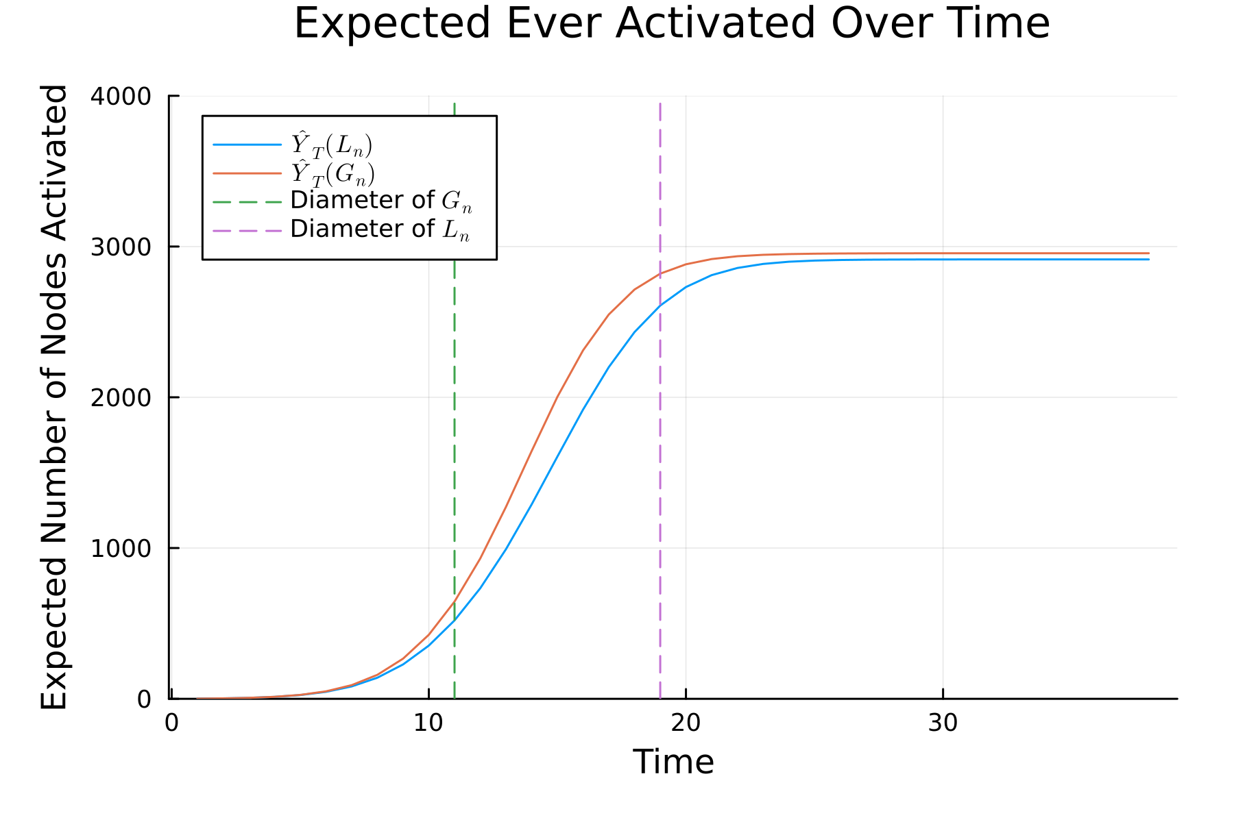
(a) $q=4$

(b) $q=2$

Figure B.1. This figure plots the same information as Figure 3, but separated by graph for both $q=4$ and $q=2$. The trajectory of $\hat{Y}_{T}(L_{n})$ initially lags behind that of $\hat{Y}_{T}(G_{n})$, leading to the decrease in the ratio shown in Figure 3. As $\hat{Y}_{T}(L_{n})$ catches up, the ratio increases.

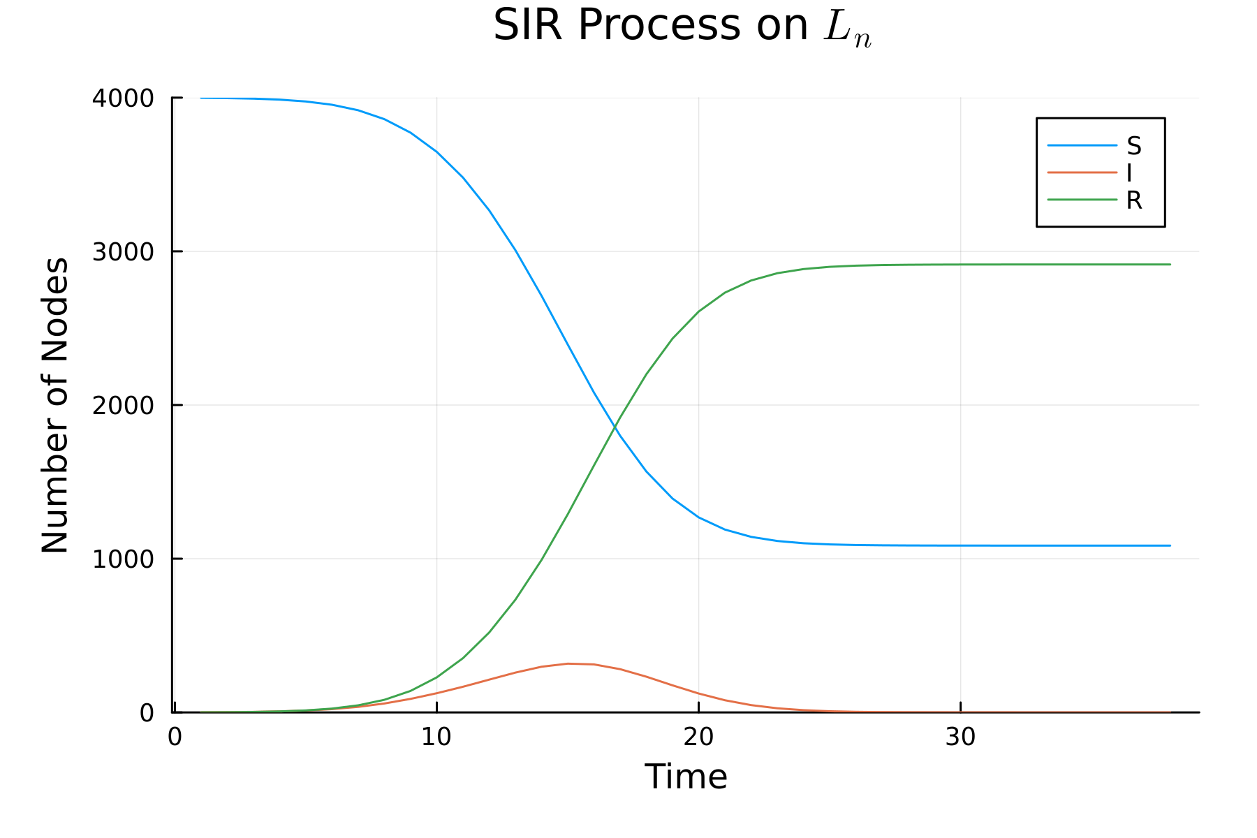
(a) $q=4$, $L_{n}$

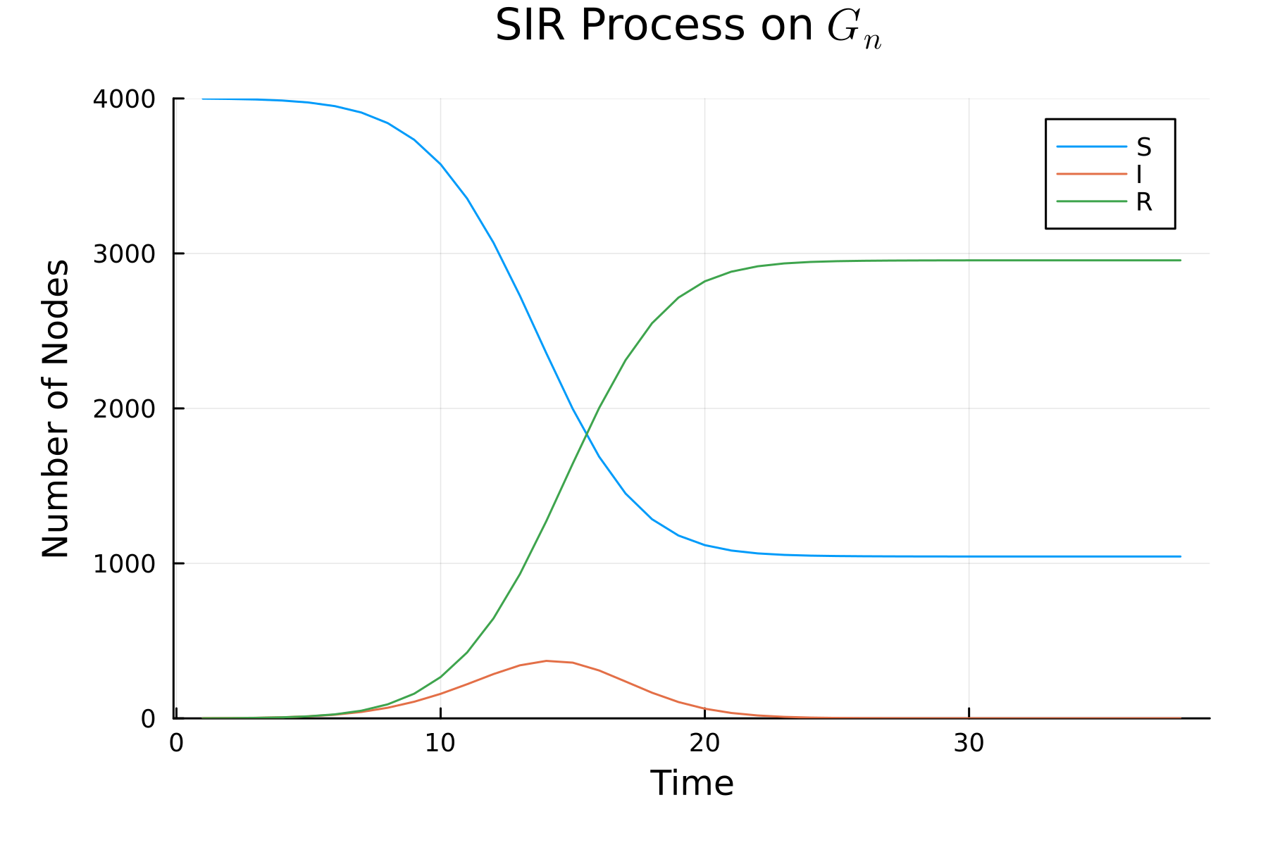
(b) $q=4$, $G_{n}$

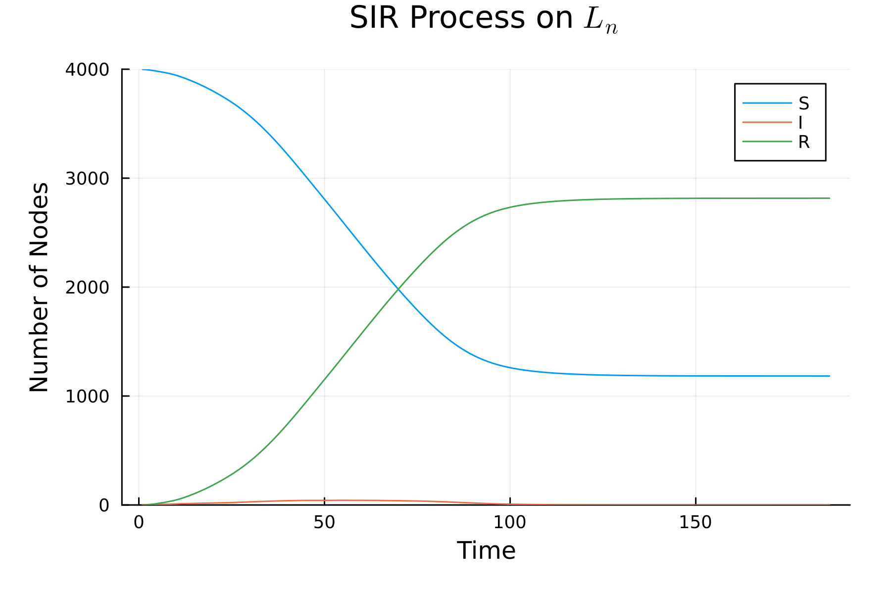
(c) $q=2$, $L_{n}$

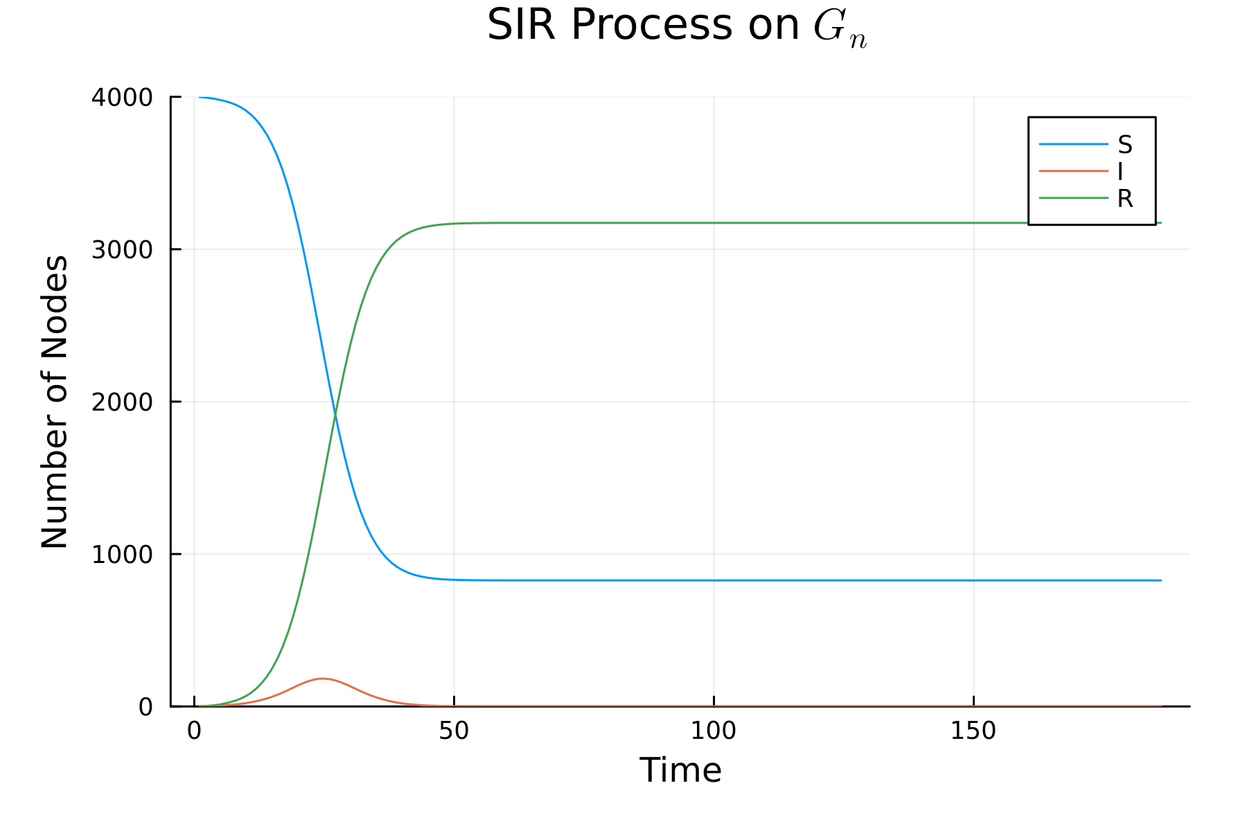
(d) $q=2$, $G_{n}$

Figure B.2. Simulations meant to emulate Theorem 1, disaggregated into the standard SIR framework. The figure is a result of averaging over simulation draws. Note that we see a larger spike in activations under $G_{n}$, which makes intuitive sense – the additional links allow for more infections to occur. We show results for both $q=4$ and $q=2$, both with $\beta_{n}=\frac{1}{10n}$. Note that the gap between total activations with $q=2$ is larger, as the additional links have a larger effect.

B.4. Simulation of Theorem 2

As an analogue to Theorem 2, we simulate SIR processes on a fixed $G_{n}$ with slightly perturbed starting points. We choose $i_{0}$ to be in the center of the lattice of $L_{n}$, that forms the backbone of $G_{n}$. Then, we build a set of alternative seeds $J_{i_{0}}$. First, we find the second distance of the closest link in $E_{n}$ – denote this $d(e_{2})$. Then, all nodes at $d(e_{2})+1$ are included in $J_{i_{0}}$. We then choose a $j_{0}\in J_{i_{0}}$ uniformly at random.

The SIR process is then run, starting at both $i_{0}$ and $j_{0}$. We record which nodes are ever activated at each step of the process, under each simulation. To follow Theorem 2, we fix the percolation across the simulation starting at $i_{0}$ and $j_{0}$. To do so, we use the fact that for a one-period SIR model, each link can transmit the disease at most one time. Therefore, we can simulate ex-ante which links will be able to transmit, which occurs with probability $p_{n}$, and intersect this with $G_{n}$ to get the realized percolation.

We then compute a standard Jaccard index to track the intersection of the two epidemics. Let $I_{P}(i_{0})$ be the set of ever-infected nodes under the epidemic from $i_{0}$, and $I_{P}(j_{0})$ be the corresponding set from $j_{0}$. Then, we compute:

$${\mathcal{J}}:={\mathbb{E}}\left[\frac{|I_{P}(i_{0})\cap I_{P}(j_{0})|}{|I_{P}(i_{0})\cup I_{P}(j_{0})|}\mid G_{n},P\right]$$

We define the Jaccard index ${\mathcal{J}}$ in a slightly different fashion than to $\Delta_{n}$, the Jaccard index in Theorem 2. Note that ${\mathcal{J}}$ is a re-arrangement of $\Delta_{n}$: the union of $I_{P}(i_{0})$ and $I_{P}(j_{0})$ contains the intersection and the disjoint set, which are the key pieces of $\Delta_{n}$. We use this index because we do not condition on the event that the epidemics have some overlap (denoted as $\Gamma_{n}$ and that there exists a path from $j_{0}$ to the second closes link to $i_{0}$ in $E_{n}$. Empirically, instances in which there is no overlap during some time periods is common, meaning that the empirical analogue of $\Delta_{n}$ will not be well defined (as the denominator will be zero). Thus, we re-arrange terms and use the standard Jaccard index ${\mathcal{J}}$. Note the due to the re-arrangement, small values of ${\mathcal{J}}$ indicate very little overlap between epidemics, similar to high values of $\Delta_{n}$.

B.5. Fitting a SIR Model

We study how a policymaker could estimate a model of the diffusion process via a standard compartmental model. Instead of the network based SIR model, we assume the policymaker estimates the parameters of a version of the standard differential equation SIR model. Changes in the number of susceptible ($S(t)$), infected ($I(t)$), and removed ($R(t)$) at time $t$ are given by:

$$\dot{S}(t):=-\frac{s}{n}S(t-1)I(t-1)$$

$$\dot{I}(t):=\frac{s}{n}S(t-1)I(t-1)-rI(t-1)$$

$$\dot{R}(t):=rI(t-1)$$

Where $s$ and $r$ are parameters that govern the disease process. Note that ${\mathcal{R}}_{0}=s/r$. This model is exactly a discrete-time analogue of the standard SIR model.

We assume that the policymaker estimates $\hat{s}$ and $\hat{r}$ from observed data via a set of moment conditions, matching both the number of infected and removed people at each time step. It will be useful to define some additional notation. Let $N$ be the number of simulations. Let $I_{n}^{s}(t)$ be the number of infected people at time $t$ in simulation $n$. Let $R_{n}^{s}(t)$ be defined analogously for recovered. Let $I(t;s,r)$ be the number of infected at time $t$ with parameters $r$ and $s$. Let $R(t;s,r)$ be defined analogously. Then, the policymaker solves the following problem for each simulation run, given $T$ periods of data. We then collect the moment conditions in the following vector:

$$M_{n}(t)=\begin{pmatrix}I_{n}^{s}(t)-I(t;s,r)\\ R_{n}^{s}(t)-R(t;s,r)\end{pmatrix}$$

Then the policymaker solves:

$$\{\hat{s}_{n},\hat{r}_{n}\}:=\text{argmin}_{s,r}\frac{1}{T}\sum_{t=1}^{T}M_{n}(t)^{\prime}M_{n}(t)$$

For each simulation. Then, we compute the following quantities, getting the average trajectory from the fitted SIR models.

$$\bar{I}(t)=\frac{1}{N}\sum_{n=1}^{N}I(t;s_{n},r_{n})$$

$$\bar{R}(t)=\frac{1}{N}\sum_{n=1}^{N}R(t;s_{n},r_{n})$$

$${\mathcal{R}}_{0}=\frac{1}{N}\sum_{n=1}^{N}\frac{s_{n}}{r_{n}}$$

We can also compare directly to the metric of average ever activated, our policy object of interest for much of the main text, by computing $\bar{I}(t)+\bar{R}(t)$ at each time period. As data, we use simulations of $\hat{Y}_{T}(L_{n})$ or $\hat{Y}_{T}(G_{n})$. We use $T/4$ periods of “data" to fit the model, and then simulate the model forward with the estimated $\hat{s}$ and $\hat{r}$. Results are discussed in the main text and in Figure 4. Additional results are shown in Figures B.3 and B.4.

For $\hat{Y}_{T}(L_{n})$, the average (across simulations) root mean squared error (RMSE) is 11.43, while with $\hat{Y}_{T}(G_{n})$ it is 11.89. Unsurprisingly, the RMSE under $\hat{Y}_{T}(G_{n})$ is larger, as the data is inherently noisier. The simulated trajectories quickly diverge from the data out of sample. In the next $T/4$ periods, the average RMSE with $\hat{Y}_{T}(L_{n})$ is 429.08, while with $\hat{Y}_{T}(G_{n})$ it is 354.21. This divergence is shown in Figure 4.

As an additional exercise, we plot the difference between the simulated forward and “true" trajectories under each data generating process. Results are shown in Figure B.3. We can note that under the true data generating process of $\hat{Y}_{T}(G_{n})$, the maximum under and over-estimation by the SIR differential equation model is smaller than under $\hat{Y}_{T}(L_{n})$. The additional i.i.d. links increase the degree of the polynomial, meaning that an exponential SIR model can more closely approximate the process. This effect is much larger with $q=2$ than with $q=4$, as this is when the SIR model approximates the process more poorly.

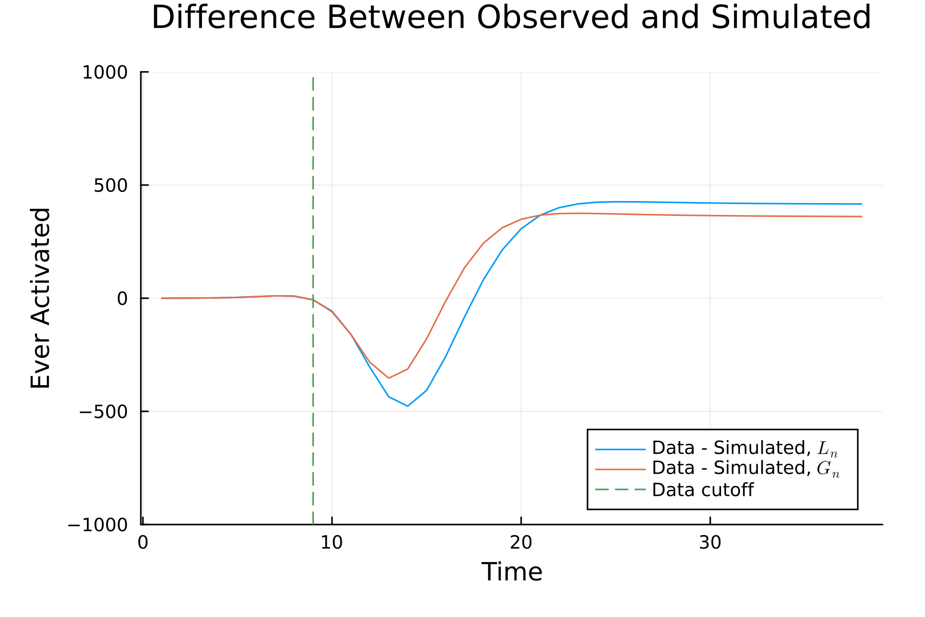
(a) $q=4$

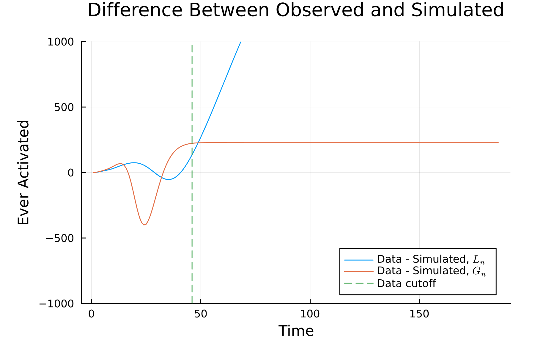
(b) $q=2$

Figure B.3. Differences between $\hat{Y}_{T}(L_{n})$ and $\hat{Y}_{T}(G_{n})$ and the fitted values from the differential equation SIR model, for both $q=4$ and $q=2$.

As discussed in the main text, Figure B.4 demonstrates that the fitted value of $\hat{\mathcal{R}}_{0}$ is typically below the true value of ${\mathcal{R}}_{0}=2.5$. In particular, with $q=2$ and $L_{n}$, the estimation procedure dramatically underestimates the true value of ${\mathcal{R}}_{0}$. As discussed in the main text, this is because the estimation procedure does not use the micro-data of exactly which nodes are activated and when, as suggested in Proposition 1.

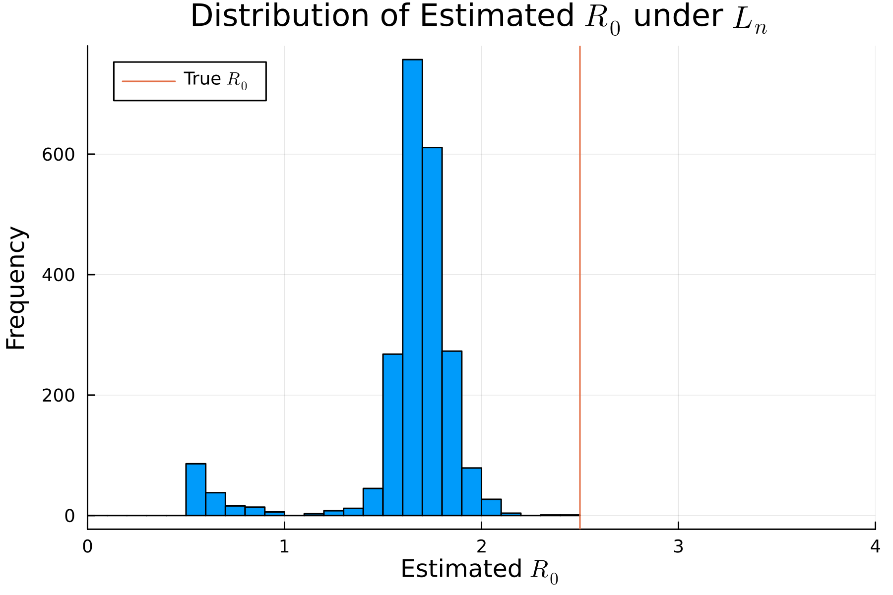
(a) $q=4$

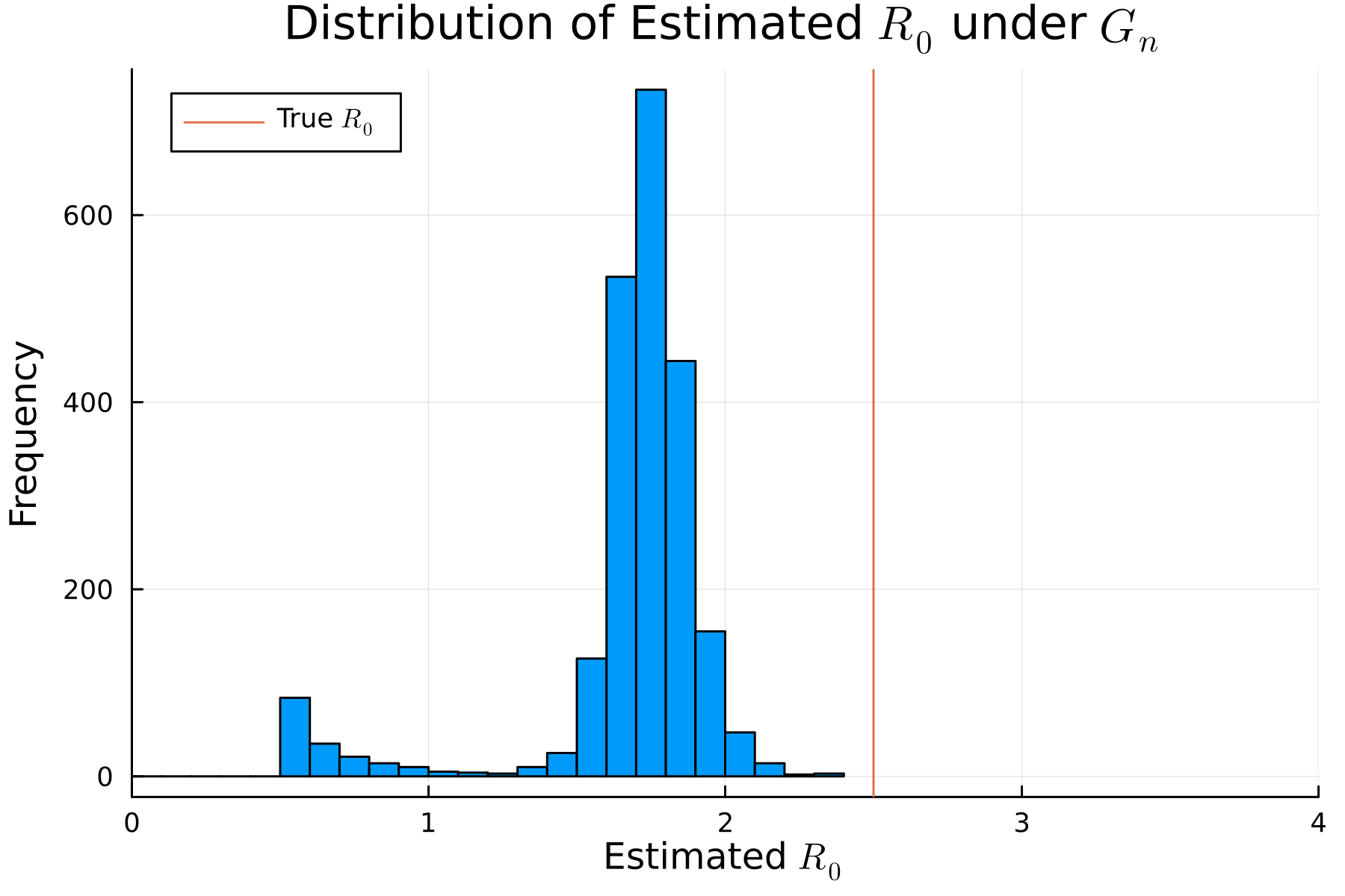
(b) $q=4$

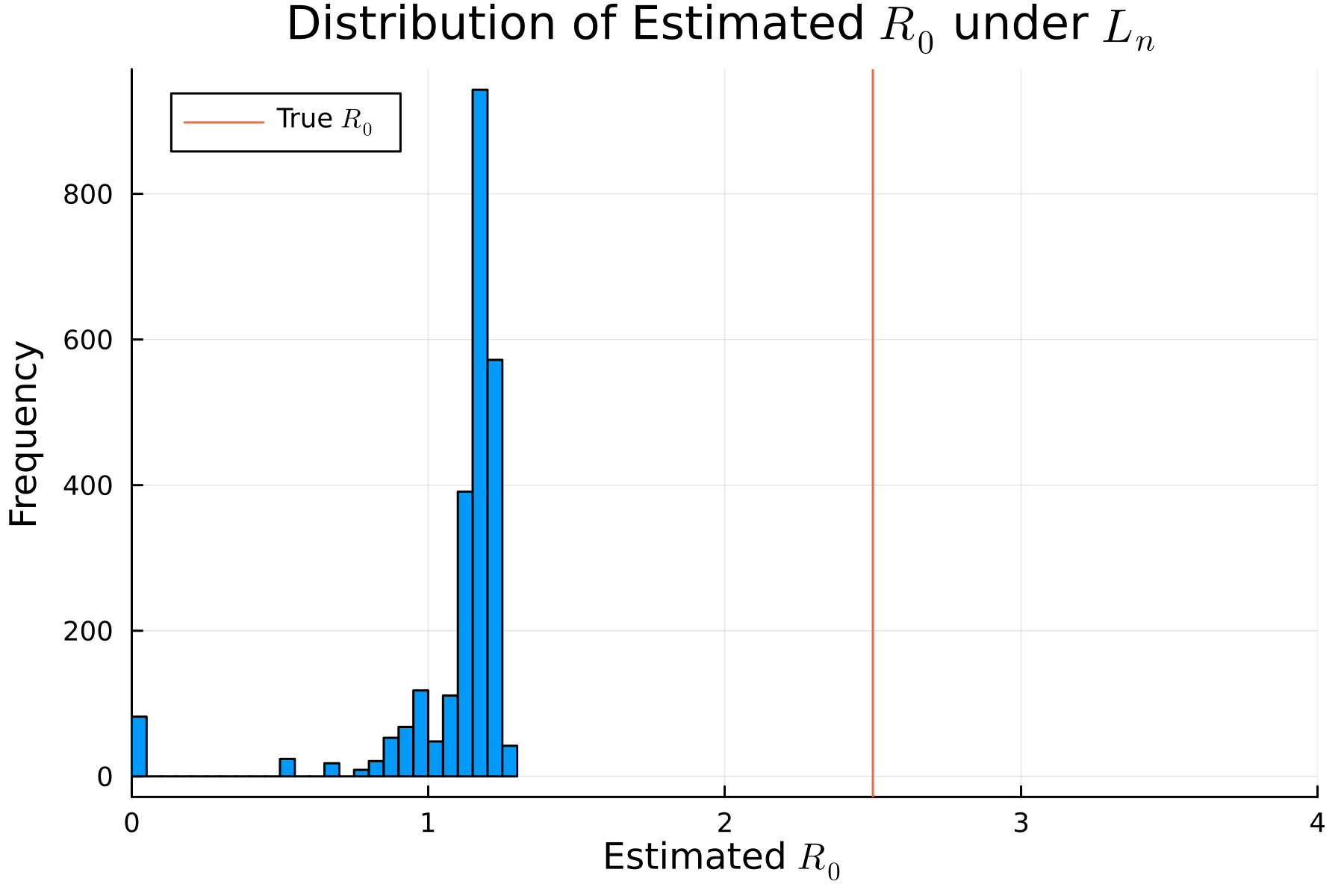
(c) $q=2$

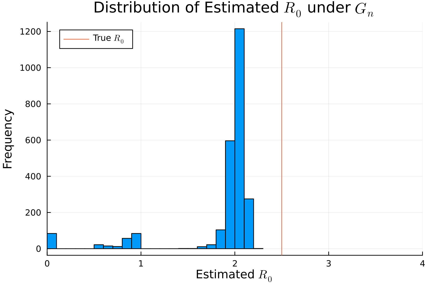
(d) $q=2$

Figure B.4. Distribution of estimated $\hat{\mathcal{R}}_{0}$ across simulations when $L_{n}$ is based on $q=4$. Note that the distribution of values sits below the true value of ${\mathcal{R}}_{0}=2.5$. Values very close to zero come from data where the epidemic stops after a very small number of activations.

B.6. Extreme Sensitivity with $q=2$

We explore an additional set of simulations in the case of $q=2$, this time using a much smaller value of $\beta_{n}=\frac{1}{100n}$. We show average graph statistics in Table B.2. Results are shown in Figures B.5.

Statistic	$L_{n}$	$G_{n}$
Dimension	2.0	2.0
Diameter	93.0	45.059
Mean Degree	5.826	5.836
Min Degree	2.0	2.0
Max Degree	16.0	16.007
Mean Clustering Coefficient	0.379	0.38
Average Path Length	31.774	18.802

Table B.2. Graph statistics for $L_{n}$ generated as in the Monte Carlo simulations with $q=2$, and $G_{n}$ generated with $\beta_{n}=\frac{1}{100n}$. Statistics for $G_{n}$ are taken as an average over 2,500 draws.

(a)

(b)

(c)

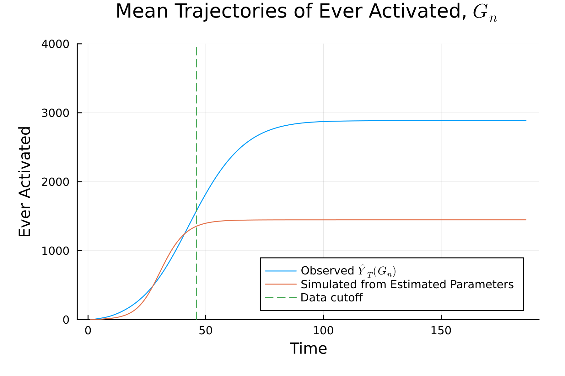
(d)

Figure B.5. Results with $q=2$ and $\beta_{n}=\frac{1}{100n}$. Panel (A) shows the ratio $\hat{Y}_{T}(L_{n})/\hat{Y}_{T}(G_{n})$, while Panel (B) shows the Jaccard index ${\mathcal{J}}$. Panels (C) and (D) show the fitted values of a SIR differential equation model, fit to $\hat{Y}_{T}(L_{n})$ and $\hat{Y}_{T}(G_{n})$. Averages are taken over 2,500 Monte Carlo simulations.

As shown in Figure B.5, despite a much smaller value of $\beta_{n}$ forecasting issues persist. The minimum value of $\hat{Y}_{T}(L_{n})/\hat{Y}_{T}(G_{n})$ is achieved at $T=46$, taking a value of 0.649. This value is still lower than the case with $q=4$ and $\beta_{n}=\frac{1}{10n}$ (which had a minimum of 0.780), showing the extreme sensitivity in the lower dimension. Note that over very short time ranges, the value of the ratio is slightly above 1 – this is a result of finite sample noise, with several diffusion processes on $L_{n}$ infecting a large number of nodes quickly, and a few processes on $G_{n}$ infecting very few nodes. For sensitive dependence, $j_{0}$ is at distance 16 from $i_{0}$: this much larger distance comes from both the clustered nature of the graph, and the lack of i.i.d. links to connect disparate locations (due to the low value of $\beta_{n}$). Because there are so few links in $E_{n}$, due to the small value of $\beta_{n}$, the local neighborhood containing all $j_{0}$ is 7.13 percent of the graph, and only 10.90 percent of the neighborhood are candidate $j_{0}$. With this in mind, it is not surprising to see the process exhibit severe sensitive dependence on the seed location: at half of the diameter of $G_{n}$ ($T=22$), the value of ${\mathcal{J}}=0.09$ on average, indicating almost totally disjoint diffusion processes.

The third and fourth panels of Figure B.5 show the compartmental SIR fitting exercise. Here, the introduction of $E_{n}$ has less of an impact, as shown by the relative similarity between the results for $L_{n}$ and $G_{n}$. This result is not surprising, given the very small value of $\beta_{n}$. Recall that we fit the SIR model to $\hat{Y}_{T}(L_{n})$ and $\hat{Y}_{T}(G_{n})$, over the first 46 time steps (corresponding to $T/4$, equivalent to half of the diameter of $L_{n}$). In the fitting period, using $\hat{Y}_{T}(L_{n})$, the average RMSE is 62.069, while in the next $T/4$ periods it is 1235.168 – a very similar set of values to the $q=2$ case in the main text. With $\hat{Y}_{T}(G_{n})$, the within sample average RMSE is 101.128, while in the next $T/4$ periods it is 1242.687. These values are much more similar to the $L_{n}$ case than the corresponding values for $q=2$ in the main text – this is because there are many fewer additional links in $G_{n}$. Therefore, while the additional links increase the dimensionality of the diffusion process, the compartmental SIR model still gives a poor approximation. As further evidence, in both cases, the compartmental model dramatically underestimates the true value of ${\mathcal{R}}_{0}=2.5$: under $L_{n}$ it is estimated as 1.10, and under $G_{n}$ it is estimated as 1.21.

Appendix C Empirical Example: Location Data from the COVID-19 Epidemic

We give a detailed description of the data processing procedures, along with additional results using a graph constructed from location data. We build a network using visitor flows based on cell phone location data, provided by SafeGraph (Kang et al.,, 2020). Our primary analysis studies the entirety of California and Nevada, with a small portion of Arizona included. Figure C.1 shows the region on a map. Note that we only include areas in the United States. The region includes major cities including San Francisco, Los Angeles, and Las Vegas.

Figure C.1. The area covered by our location flows data. We study only Census tracts within the United States. Figure taken from Google Maps.

We work with Census tracts as the unit of observation, which each contain approximately 4,000 people. Given privacy concerns, we focus on movement between tracts, rather than tracking individual people. We use tract-to-tract flows on March 1st, 2020. This date was before the WHO declared COVID-19 a pandemic, and before the United States government declared a national state of emergency.

We construct graphs in the following manner. Fix a cutoff $c$. Then we take the following steps.

1. For each pair of Census tracts $a$ and $b$, we construct the average flow between tracts by taking the average of the flow from $a$ to $b$ and the flow from $b$ to $a$. Call this value $f_{ab}$.

2. Tracts $a$ and $b$ will be linked in the graph only if $f_{ab}>c$.

We choose $c$ based on the empirical distribution of $f_{ab}$, the flows between tracts. We refer to this procedure as “pruning." If the process results in a disconnected graph, we choose the largest connected subgraph. As before, we set $T$ as twice the diameter of $L_{n}$.

C.1. Disease Process

As with the simulated graphs, we fix ${\mathcal{R}}_{0}=2.5$. We then compute $p_{n}={\mathcal{R}}_{0}/\bar{d}$, where $\bar{d}$ is the average degree in $L_{n}$. Note that in this case, the meaning of ${\mathcal{R}}_{0}$ is substantively different – because nodes now refer to Census tracts, infecting 2.5 nodes in the disease free state on average means infected 2.5 tracts on average.

C.2. Errors Induced by Cutoff Choice

We first study errors induced by choosing different cutoffs for pruning the graph. We construct $G_{n}$ by setting $c=5$, which is at the 91st percentile of the empirical distribution of tract-to-tract flows. Then, we generate $L_{n}$ by choosing $c=6$. Note that every link in $L_{n}$ will be in $G_{n}$, meaning that we can construct the implied error graph $E_{n}$.

We conduct the same three analyses that we did with the simulated graph. First, we study a version of Theorem 1, comparing the expected number of infections on each graph. Second, we study a version of Theorem 2, comparing the overlap between epidemics after perturbing the starting point. Finally, we consider the exercise of fitting a SIR differential equation model.

For the sake of brevity, we only note differences unique to this section when compared to the procedures discussed in Section B. When considering the simulation of Theorem 1, the key change is that we hold $G_{n}$ fixed: it is generated once from the data. When we take expectations, they are taken only over the disease process only. Otherwise, the process is identical. When considering the simulation of Theorem 2, the only change is how $i_{0}$ is selected – we set $i_{0}$ to be the node with the highest degree in $G_{n}$. The process of fitting a differential equation SIR model is exactly as before. In addition, we conduct simulations with $E_{n}$ taken to be an Erdos-Renyi random graph, rather than via the pruning procedure. In the main text, we set $\beta_{n}$ so that the i.i.d. errors generate the same expected volume of links as the pruning procedure. As an additional set of results, we set $\beta_{n}=\frac{1}{10n}$, to compare with the Monte Carlo simulations. Summary statistics of the resulting graphs are shown in Table C.1.

Statistic	$L_{n}$	$G_{n}^{92}$	$G_{n}^{\beta}$
Error Type	—	Pruned	IID
Diameter	21.0	15.0	7.687
Mean Degree	12.962	15.486	16.172
Min Degree	1.0	1.0	1.839
Max Degree	298.0	329.0	301.148
Mean Clustering Coefficient	0.389	0.393	0.234
Average Path Length	7.253	5.866	4.03

Table C.1. Graph statistics for $L_{n}$ and both hypothetical $G_{n}$s constructed from California, Nevada, and Arizona Census tract flow data. Statistics for $G_{n}^{\beta}$ with i.i.d. errors are averaged over 2,500 draws.

C.3. Additional Results

We again estimate the compartmental SIR model using the simulated epidemics above. This process is identical to the procedure conducted in Section 6.1. One pattern of note is that the model fit to $\hat{Y}_{T}(G_{n})$ generated from the pruning procedure underestimates the average number of infections, while the model fit to $\hat{Y}_{T}(L_{n})$ overestimates.

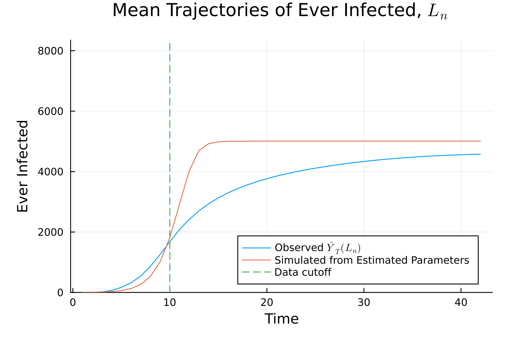
(a) Pruned

(b) Pruned

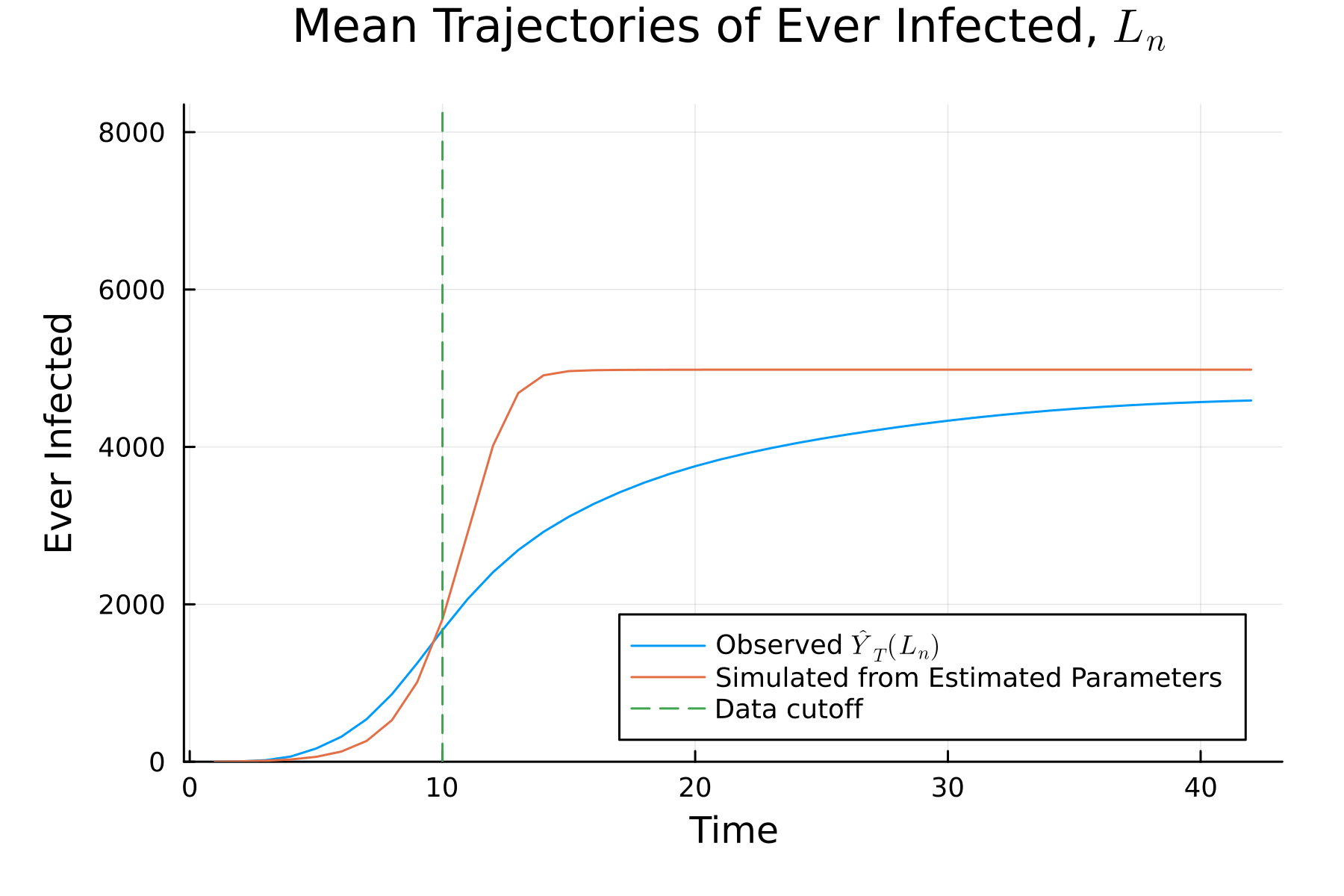
(c) I.I.D.

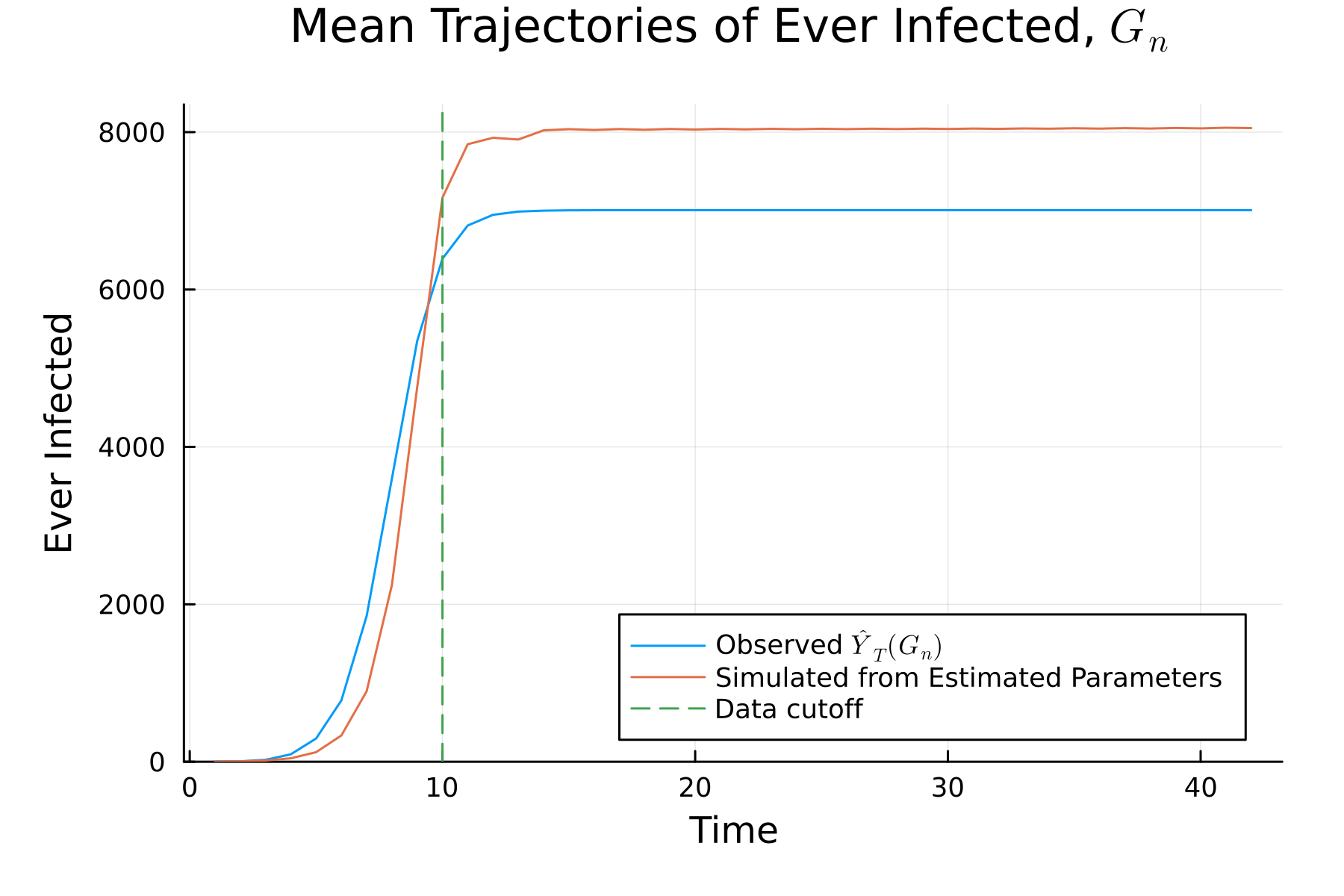
(d) I.I.D.

Figure C.2. A comparison of the mean ever infected under the true network SIR model and the estimated trajectory from the differential equations model. Here, $L_{n}$ is generated from location flow data in California, Nevada, and a portion of Arizona. Panel (A) and (B) use the pruning procedure, while (C) and (D) have i.i.d. links. Panel (A) shows simulations when $\hat{Y}_{T}(L_{n})$ is used as the data generating process, while Panel (B) shows when $\hat{Y}_{T}(G_{n})$ is used. The data cutoff is at $T/4$. Before this point, the SIR model is fit to the data via the generalized method of moments. After this point, we run the differential equation model forward to see how it performs out of sample.

In the estimation period before $T/4$, the RMSE for $\hat{Y}_{T}(L_{n})$ is 202.98, while in the next $T/4$ periods it is 1953.41. When fit to $\hat{Y}_{T}(G_{n}^{93})$, the RMSE in the first $T/4$ periods is 452.09, while in the next $T/4$ periods it is 1320.60. Notably, the model has a much better fit out of sample for $G_{n}^{93}$. For the i.i.d. errors on $G_{n}^{\beta}$, the results are similar. In the estimation period, the RMSE fitted to $\hat{Y}_{T}(L_{n})$ is 200.541, while in the next $T/4$ periods it is 1944.63. When fit to $\hat{Y}_{T}(G_{n})$, the RMSE in the first $T/4$ periods is 700.93, while in the next $T/4$ periods it is 1095.14.

We then show a set of additional figures, corresponding to the simulations from the main text. We first disaggregate the simulated diffusion processes into a standard SIR framework, as shown in Figure C.3. Second, we show the distribution of estimated $\hat{\mathcal{R}}_{0}$ across simulations in Figure C.4. Figure C.3 demonstrates that with i.i.d. errors, the infection profile is relatively sharp, as the epidemic quickly expands to cover the whole graph during the intermediate range of $T$.

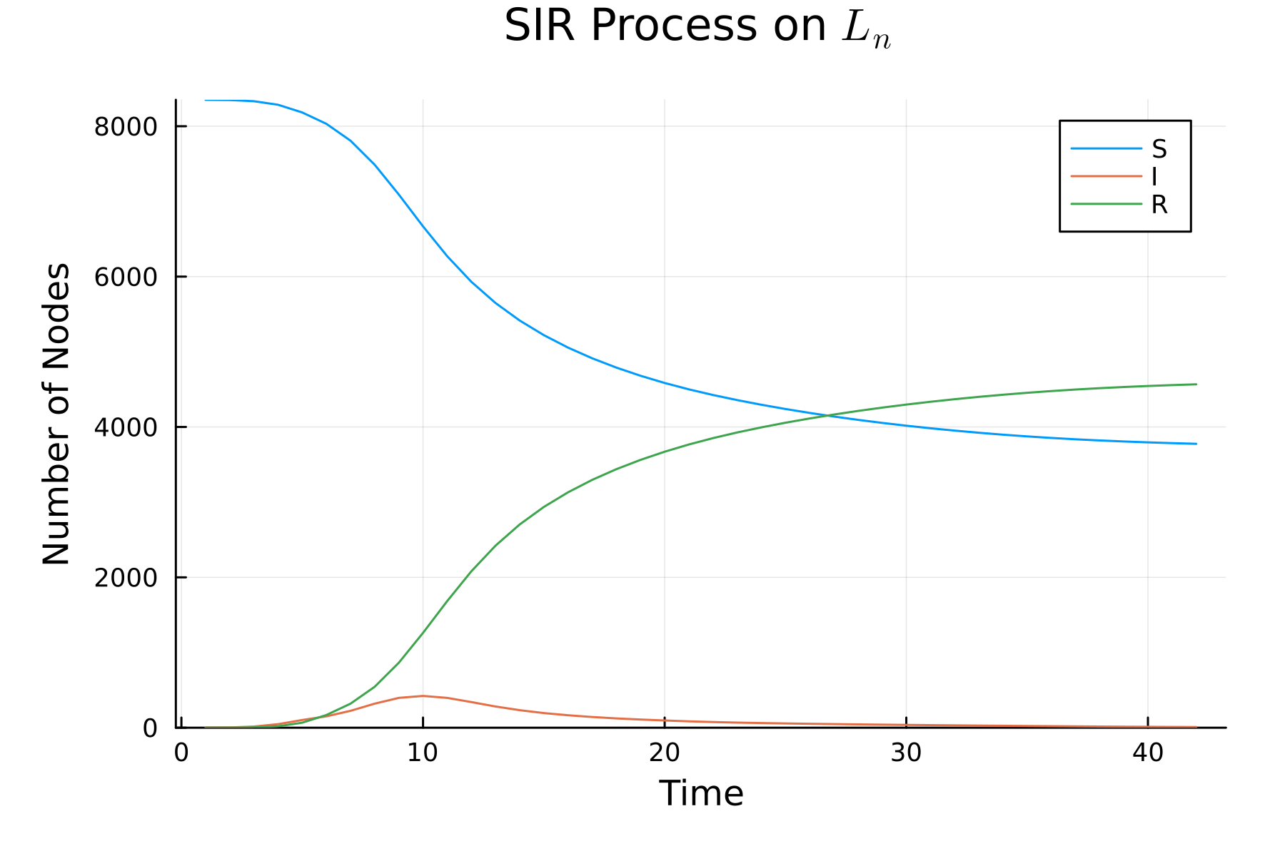
(a)

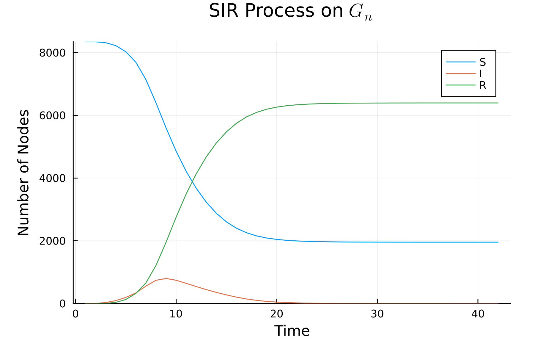
(b) Pruned

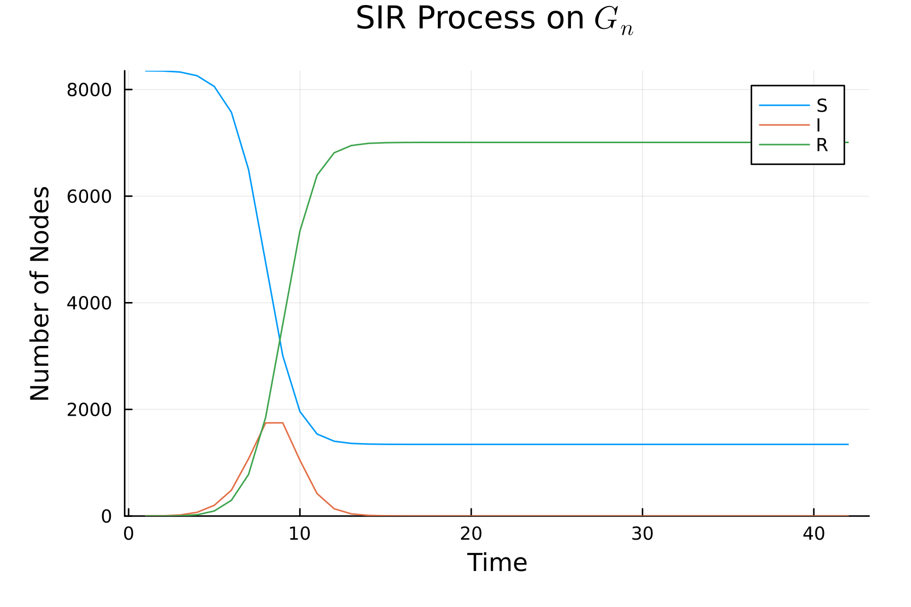
(c) I.I.D.

Figure C.3. Trajectories of $\hat{Y}_{T}(L_{n})$ and $\hat{Y}_{T}(G_{n})$ disaggregated into the standard SIR curves for $L_{n}$ and $G_{n}$ for each scenario. Note that the $L_{n}$ specifications are identical, as it is exactly the same graph.

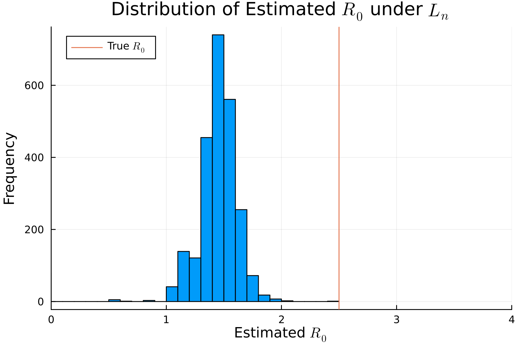
(a)

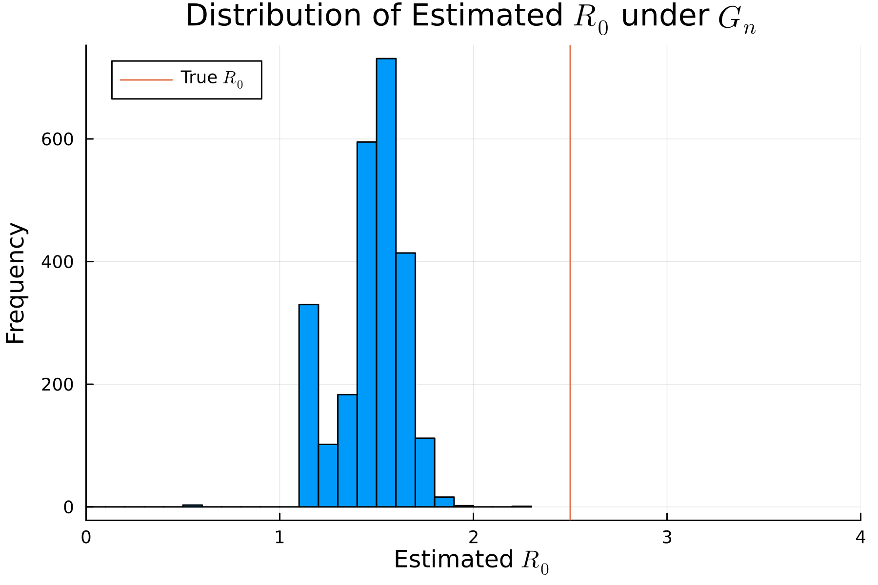
(b) Pruned

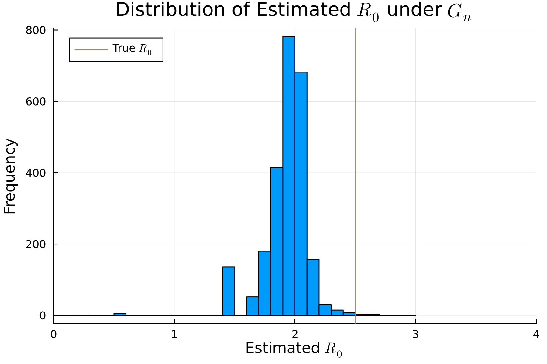
(c) I.I.D.

Figure C.4. The distribution of values of $\hat{\mathcal{R}}_{0}$ estimated when fitting the compartmental SIR model to the COIVD-19 travel data.

C.4. Lower Rates of I.I.D. Errors

To make a more direct comparison to the Monte Carlo simulations, we repeat the simulation exercises using $E_{n}$ generated i.i.d. with $\beta_{n}=\frac{1}{10n}$. Graph statistics are shown in Table C.2, again for $L_{n}$ and the average statistics for $G_{n}$ over 2,500 draws of $E_{n}$. Compared to $G_{n}$ in the main text (in Table C.1), note that the change in degree, clustering, and average path length are all much smaller, as $E_{n}$ is much more sparse in this case.

Statistic	$L_{n}$	$G_{n}$
Diameter	21.0	16.874
Mean Degree	12.962	13.062
Min Degree	1.0	1.0
Max Degree	298.0	298.106
Mean Clustering Coefficient	0.388	0.38
Average Path Length	7.295	6.116

Table C.2. Average graph statistics with i.i.d. errors in the travel data for California, Nevada, and a small portion of Arizona. $G_{n}$ is generated from $L_{n}$ using i.i.d. additional links, which occur with $\beta_{n}=\frac{1}{10n}$

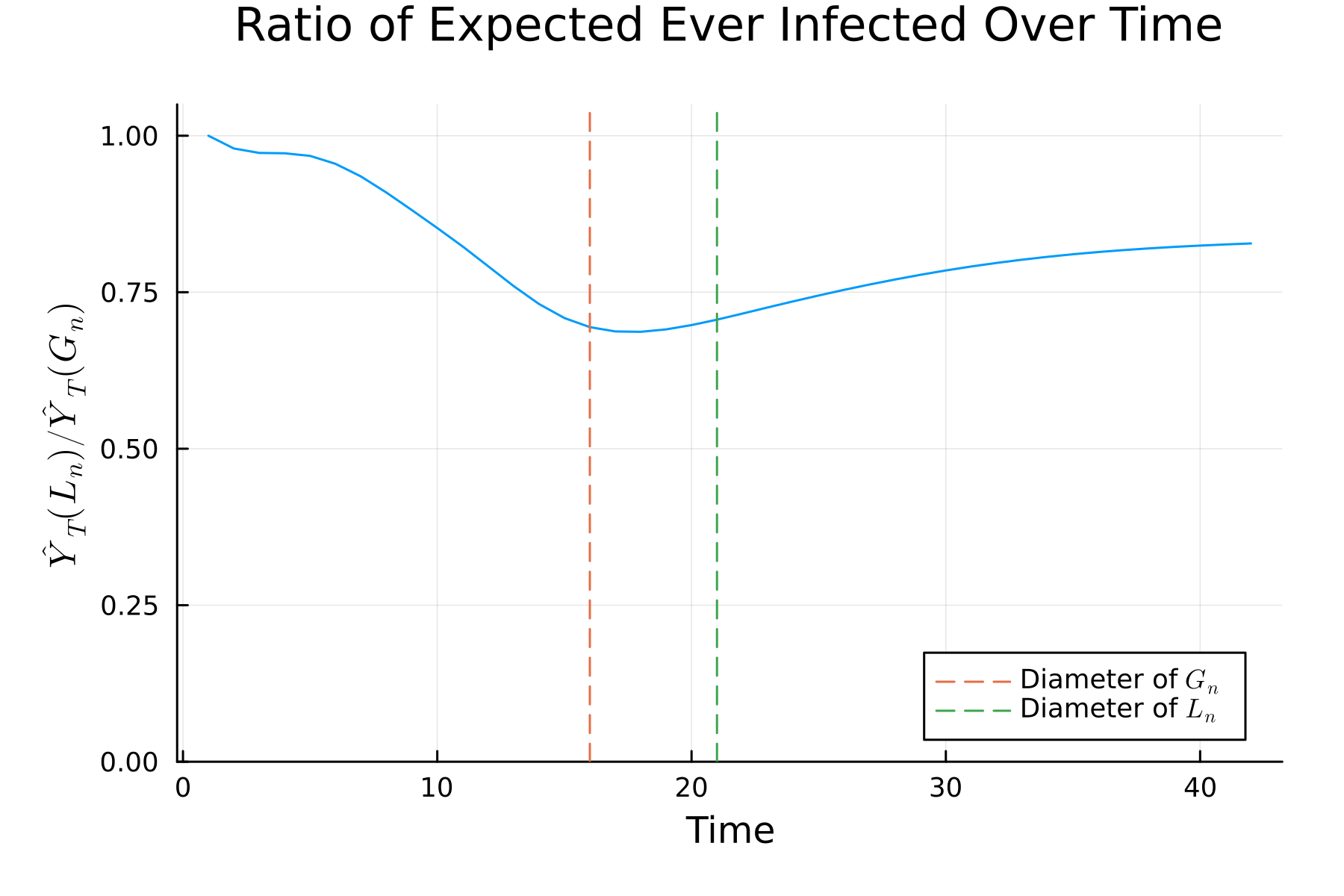
(a)

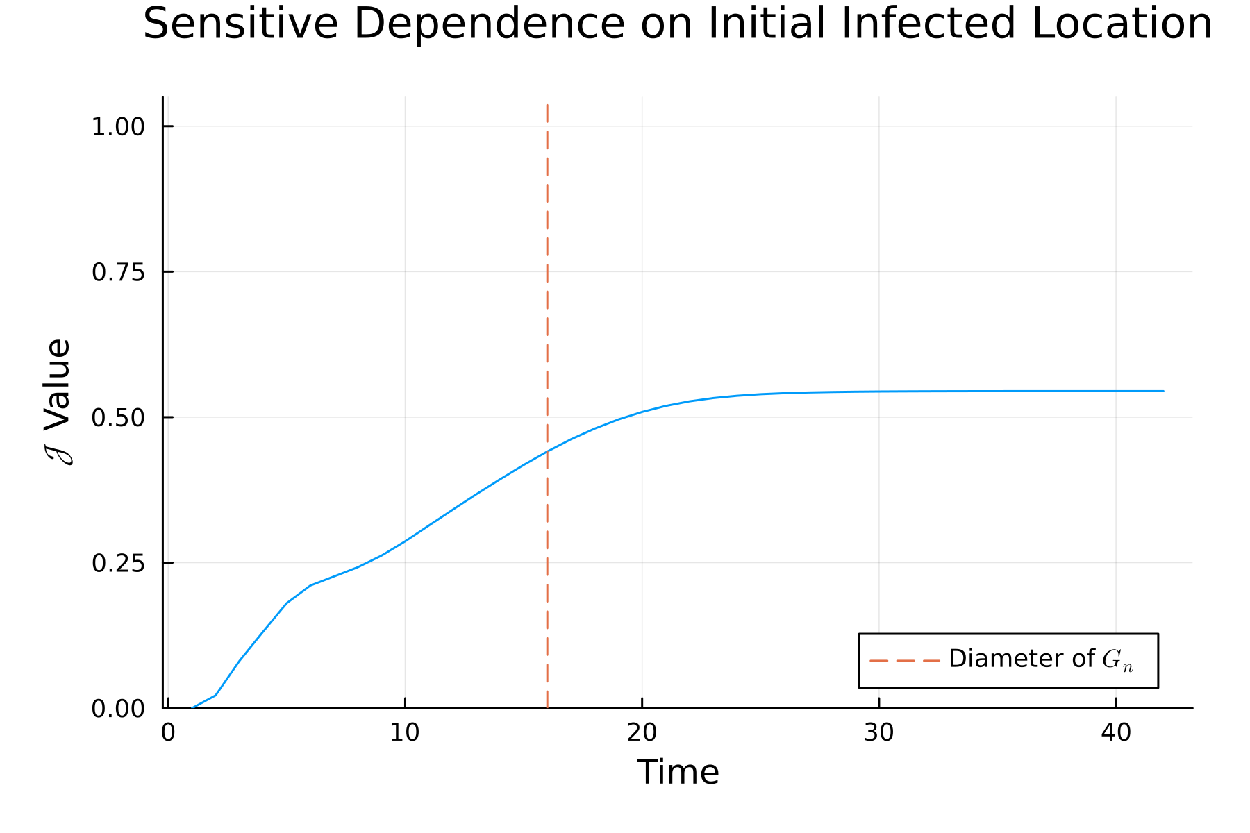
(b)

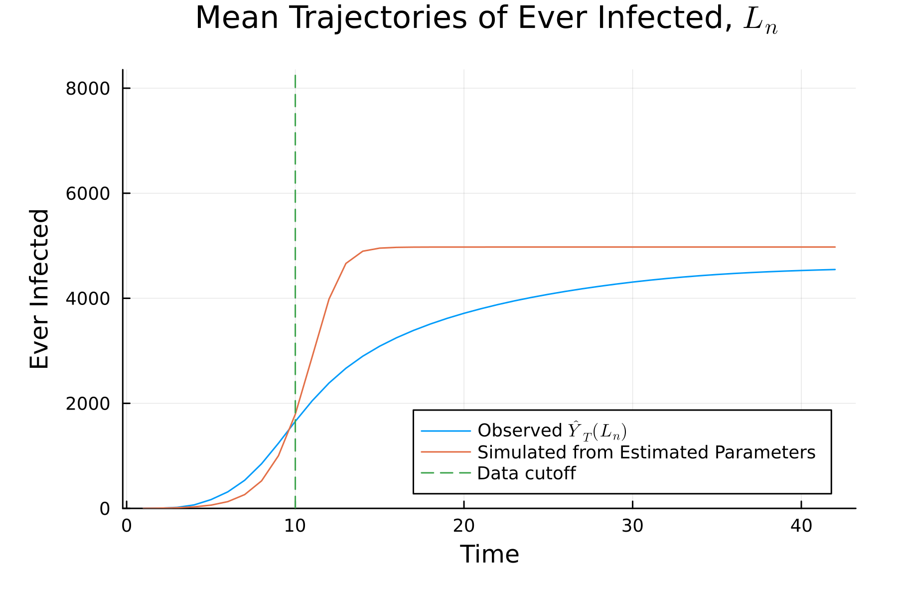
(c)

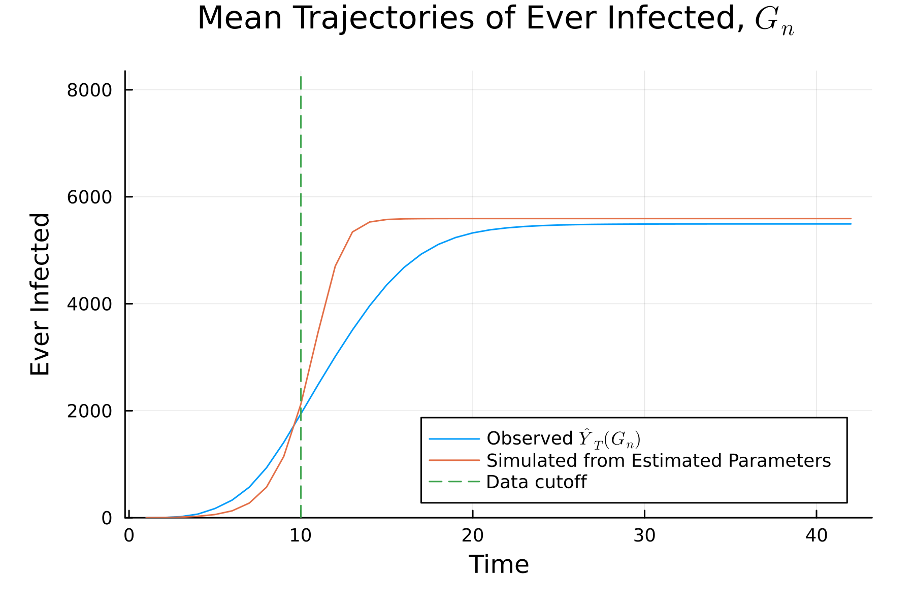
(d)

Figure C.5. Results using the COVID-19 travel data, with $G_{n}$ using $E_{n}$ generated i.i.d. with $\beta_{n}=\frac{1}{10n}$. Panel (A) shows the ratio $\hat{Y}_{T}(L_{n})/\hat{Y}_{T}(G_{n})$, while Panel (B) shows the Jaccard index ${\mathcal{J}}$. Panels (C) and (D) show the fitted values of a SIR differential equation model, fit to $\hat{Y}_{T}(L_{n})$ and $\hat{Y}_{T}(G_{n})$. Averages are taken over 2,500 Monte Carlo simulations.

Results are shown in Figure C.5. We take averages over 2,500 simulations. The first panel shows the simulation of Theorem 1. Note that in this case, the minimum ratio of $\hat{Y}_{T}(L_{n})/\hat{Y}_{T}(G_{n})$ is achieved at $T=18$ and takes the value 0.686. This value is much larger than the values from the main text with either the pruned or i.i.d. errors, and comparable to the values with the same level of $\beta_{n}$ and graph dimension $q=4$ in the Monte Carlo simulations. The second panel shows the simulation of Theorem 2. As in the main text, we choose the local neighborhood containing all $j_{0}$ conservatively: we chose the set to be all nodes within distance 2 of $i_{0}$. The distance from $i_{0}$ to $j_{0}$ is therefore 2, and the neighborhood that contains all possible $j_{0}$ contains 0.80 percent of the graph. Of the neighborhood, 89.55 percent of the nodes are candidates for $j_{0}$. Halfway to the diameter of $G_{n}$, the value of the average Jaccard index is 0.24, indicating largely distinct epidemics.

The third and fourth panels of Figure C.5 show the fitted compartmental SIR models, relative to $\hat{Y}_{T}(L_{n})$ and $\hat{Y}_{T}(G_{n})$. As before, the compartmental model underestimates the true ${\mathcal{R}}_{0}=2.5$: under $\hat{Y}_{T}(L_{n})$, it estimates a value of $1.40$, and under $\hat{Y}_{T}(G_{n})$ estimates a value of 1.49. In the first $T/4$ periods, in sample, the average RMSE under $\hat{Y}_{T}(L_{n})$ is 198.96. In the next $T/4$ periods, it is 1,966.58. Under $\hat{Y}_{T}(G_{n})$, in sample, the average RMSE is 222.11, whereas in the next $T/4$ periods it is 1389.65. Similar to the Monte Carlo exercise, we see that the additional links in $E_{n}$ help increase the dimensionality of the epidemic, leading to a better fit with the exponential compartmental model.

Appendix D Empirical Example: Diffusion in Mobile Phone Marketing

We use data from Banerjee et al., (2019) as an additional empirical example of our diffusion results. We build 69 separate village graphs, by composing networks based on survey data from Karnataka, India. We have a number of directed networks:

1. Relative

2. Give advice: does the household $i$ give advice to household $j$

3. Seek advice: does household $i$ get advice from household $j$

4. Go to visit: does household $i$ visit household $j$ in free time

5. Come to visit: does household $i$ come visit household $j$ in free time

6. Borrow: does $i$ borrow kerosene or rice from household $j$

7. Lend: does $i$ lend kerosene or rice to household $j$

To construct a set of undirected networks for each village, we take the union of these seven networks. Links are assumed to be undirected, and the network is made symmetric. This network data comes from a sequence of studies conducted in Karnataka, India. We use the 2012 data in our setting, the more recent of two waves of data collection. Graph statistics are shown in Table D.1.

Statistic	$L_{n}$	$G_{n}$
Nodes	196.072	196.072
Diameter	7.087	6.787
Mean Degree	6.541	6.849
Min Degree	1.0	1.004
Max Degree	25.71	26.219
Mean Clustering Coefficient	0.228	0.199
Average Path Length	3.303	3.168

Table D.1. Average village graph information from Banerjee et al., (2019). For $L_{n}$, averages are taken across the 69 villages in our sample. For $G_{n}$, averages are taken across the 69 villages and 2,500 draws of $E_{n}$, where $E_{n}$ is generated with $\beta_{n}=\frac{1}{2n_{v}}$ in each village separately, where $n_{v}$ is the number of households in the village.

Appendix E Empirical Example: Peer Effects in Insurance

We use data from Cai et al., (2015) to investigate an example with peer effects in a diffusion setting. In order to encourage weather insurance, a valuable product with low takeup in rural China, the researchers conducted two waves of information sessions.

To construct network data, we use the list of directed links given in their data along with additional survey data. We drop some households who are listed in the network data but not in the additional survey data – we assume that this is a result of attrition between the surveys. We then transform the directed network in each village into an undirected network: if household $i$ lists household $j$ as a friend, or vice versa, we link $i$ to $j$.

We use the same definition of treatment as in Cai et al., (2015). A household is considered to be treated if they participate in an intensive information session in the first wave of the experiment. We then compute diffusion exposure using these households as seeds. When we estimate the effect of diffusion exposure, we include only households that did not participate in the first wave of the information sessions. This procedure is consistent with the prior research.

In addition, we include a number of controls to be in line with the original paper. We control for the head of household gender, age, education, and area of rice production. In addition, following the approach in Cai et al., (2015), we control for degree to address potential concerns about selection on household sociability. Finally, we include village fixed effects. Tables E.1 and E.2 report graph summary statistics for all values of $k$ for the Monte Carlo simulations conducted in the main text.

Graph Statistic	Value
Nodes	104.30
Min Degree	0.40
Max Degree	15.79
Mean Degree	6.51
Components	5.60
Average Path Length	3.59
Diameter	8.06
Local Clustering	0.30
Exposure	0.99

Table E.1. Average graph statistics from Cai et al., (2015). Averages are taken over the 47 villages in the data. When there are multiple components, paths of infinite length (when nodes are disconnected from one another) are ignored. Mean exposure is computed before standardizing to have mean zero and standard deviation one, as we do in the regressions.

k	Min Deg	Max Deg	Mean Deg	Comp.	Path Length	Diameter	Clustering	Exposure
-	0.38	13.32	5.60	5.60	3.59	8.06	0.30	1.10
15.00	0.37	13.19	5.54	5.63	3.61	8.10	0.29	1.10
14.00	0.37	13.19	5.53	5.64	3.61	8.10	0.29	1.10
13.00	0.37	13.17	5.53	5.64	3.61	8.10	0.29	1.10
12.00	0.37	13.16	5.52	5.64	3.61	8.11	0.29	1.10
11.00	0.37	13.15	5.51	5.65	3.61	8.11	0.29	1.10
10.00	0.37	13.13	5.51	5.65	3.62	8.12	0.29	1.10
9.00	0.37	13.11	5.49	5.66	3.62	8.12	0.29	1.10
8.00	0.36	13.09	5.48	5.67	3.62	8.13	0.29	1.10
7.00	0.36	13.05	5.46	5.68	3.62	8.14	0.29	1.10
6.00	0.36	13.01	5.44	5.69	3.63	8.15	0.29	1.09
5.00	0.35	12.95	5.40	5.71	3.64	8.17	0.28	1.09

Table E.2. Graph statistics for the average graph $L_{n}$ generated by dropping links with i.i.d. probability $\beta_{n}=\frac{1}{kn_{v}}$ in each village. “Comp." stands for number of components

Appendix F Decaying Diffusion

Assumption F.1 (Polynomial Diffusion Process).

For some constant $q>1$ and all discrete-time $t$, ${\mathcal{E}}_{t}=\Theta(t^{q+1})$ and ${\mathcal{S}}_{t}={\mathcal{E}}_{t}-{\mathcal{E}}_{t-1}=\Theta(t^{q})$. Furthermore, let $p_{n}(T)=\frac{p_{n,0}}{T^{\lambda}}$ for some constant $0<\lambda<q$ and $p_{n,0}\in\left(\left(\frac{1}{\log n}\right)^{\frac{q}{2q+2}},1\right]$.

Here, we assume that diffusion decays over time, governed by the constant $\lambda$. We assume that diffusion decays at a polynomial rate. It will follow that we only have expected diffusion through links in $E_{n}$ if $\lambda<q$. In the case where $p_{n}(T)$ were to decay exponentially quickly, it would then follow we still would not have expected diffusion through $E_{n}$. With fast decay on $p_{n}(T)$, the missing links do not have a large impact because the diffusion process just dies before hitting regions that cause lots of damage.

To compare to the assumption with homogeneous $p_{n}(T)$, we note that the graph classes that are allowed under the homogenous $p_{n}$ are still valid here, with sufficiently slow decay of $p_{n}$. For example, again consider a latent space network where nodes form links locally in a Euclidean space with dimension $q$. Since volumes in Euclidean space expand at a polynomial rate and for $\lambda<q$, this ensures that Assumption F.1 will be satisfied.

Assumption F.2 (Forecast Period).

We impose that the sequence $T_{n}$ has for each $n$, $T_{n}\in[\underline{T}_{n},\overline{T}_{n}]$ where the following holds:

1. $\overline{T}_{n}=\min\left\{n^{\frac{1}{q+1}},\left(\frac{n}{p_{n,0}}\right)^{\frac{1}{q-\lambda}}\right\}$

2. $\underline{T}_{n}=(p_{n,0}\log n)^{\frac{1}{q+\lambda+2}}$.

Again, the assumption is very close to that of the main text, adapting the constants to deal with the decaying diffusion rates. We can note that the time frame considered will generally start earlier, but also potentially end earlier.

Assumption F.3.

$\beta_{n}\in\left(\frac{1}{np_{n,0}T^{q-\lambda}},\frac{1}{n}\right)$

Compared to the homogeneous diffusion rate case where we assume $\beta_{n}\in\left(\frac{1}{np_{n,0}T^{q}},\frac{1}{n}\right)$, with decaying $p_{n}(T)$ we impose a larger missing link rate. Under these conditions, a similar result to Theorem 1 holds.

Theorem F.1.

Under Assumptions F.1, F.2, and F.3, as $n\rightarrow\infty$, $\frac{\hat{Y}_{T}(L_{n})}{\hat{Y}_{T}(G_{n})}\rightarrow 0.$

This result forms a direct analogue of Theorem 1, but with a decaying diffusion rate.

Proof of Theorem F.1.

Following similar proof as in the proof of Theorem 1 Recall that

$$\hat{Y}_{T}(L_{n})={\mathcal{E}}_{t}={\mathbb{E}}\left|\{x\in L_{n}\mid x\textrm{ ever activated by the diffusion on }L_{n}\}\right|.$$

We can then bound this quantity from above using Assumption F.1.

Then we again use the tiling strategy. As in the proof of Theorem 1, we build a tiling such that the following holds. We define ${\mathcal{X}}_{T}$ as the number of tiles that are activated in time step $T$. We impose the following condition in the construction of the tiling for some constant $C\in[0,1)$:

$$C\leq\frac{\sum_{t=1}^{T-1}{\mathcal{X}}_{t}}{K}$$

for all $T$.

For the sake of tractable computations, we construct a lower bound by only tracking diffusion spread in each tile that is the result of the first seed in each tile. As before, our tiling assumptions mean that the computation reduces to:

For this simplified computation, we can compute, for $T\geq 1$:

$${\mathcal{X}}_{T} \approx\beta_{n}p_{n}n\sum_{t=0}^{T-1}{\mathcal{X}}_{t}{\mathcal{S}}_{T-t}$$

where the approximation holds up to a constant by the construction of the tiling. Note that this incorporates the effective $p_{n}$ at each step (scaled by $t^{\lambda}$ as appropriate).

To proceed with the computations, we begin by working with the recursive definition of ${\mathcal{X}}_{T}$. We can begin by substituting in:

$${\mathcal{X}}_{T} =\beta_{n}\frac{p_{n,0}}{T^{\lambda}}n\sum_{t=0}^{T-1}{\mathcal{X}}_{t}(T-t)^{q}$$

$$=\beta_{n}\frac{p_{n,0}}{T^{\lambda}}n\left[T^{q}+\sum_{t=1}^{T-1}\left(\beta_{n}\frac{p_{n,0}}{t^{\lambda}}n\sum_{s=0}^{t-1}{\mathcal{X}}_{s}(t-s)^{q}\right)(T-t)^{q}\right]$$

$$=\beta_{n}n\frac{p_{n,0}}{T^{\lambda}}\left[T^{q}+\sum_{t_{1}=1}^{T-1}(T-t_{1})^{q}\left(\beta_{n}\frac{p_{n,0}}{t_{1}^{\lambda}}n\left[t_{1}^{q}+\sum_{t_{2}=1}^{t_{1}-1}(t_{1}-t_{2})^{q}\left(\beta_{n}\frac{p_{n,0}}{t_{2}^{\lambda}}n\times...\right)\right]\right)\right]$$

The lead term of the polynomial will be $T^{q-\lambda}\beta_{n}np_{n,0}$. From here, we can plug into the above formulas. Recall that we have the following:

$$\hat{Y}_{T}(G_{n}) =T^{q+1}+\sum_{s=0}^{t-1}{\mathcal{X}}_{s}(T-s)^{q+1}$$

$$\geq T^{q+1}+\beta_{n}p_{n,0}n\sum_{s=0}^{T-1}s^{q-\lambda}(T-s)^{q+1}$$

$$\geq T^{q+1}+\frac{1}{2^{2q-\lambda+1}}\beta_{n}p_{n,0}nT^{2q-\lambda+1}$$

where the second bound comes from taking only the term corresponding to $\frac{T}{2}$ from the sum, which will be the largest individual term.

Now we can consider our object of interest using these bounds:

$$\frac{\hat{Y}_{T}(L_{n})}{\hat{Y}_{T}(G_{n})} \leq\frac{T^{q+1}}{T^{q+1}+\frac{1}{2^{2q-\lambda+1}}\beta_{n}p_{n,0}nT^{2q-\lambda+1}}$$

$$=\frac{1}{1+\frac{1}{2^{2q-\lambda+1}}\beta_{n}p_{n,0}nT^{q-\lambda}}$$

where we look at only the largest term in the denominator, noting that all terms are positive. Then, by Assumption F.3, as $\beta_{n}>\frac{1}{np_{n,0}T^{q-\lambda}}$, this quantity will go to $0$ as $n\rightarrow\infty$ and $T\rightarrow\infty$.

We next verify compatibility with Assumption F.2. First, note that to have links in $E_{n}$, in expectation, we must have:

$$\frac{p_{n,0}}{T^{\lambda}}T^{q}<n\Rightarrow T<\left(\frac{n}{p_{n}}\right)^{\frac{1}{q-\lambda}}$$

Second, recall the assumption we made in the tiling: we have to be able to divide $L_{n}$, the base graph, into enough tiles. We can collect the relevant conditions:

$$K(T,n)\geq\sum_{t=0}^{T-1}{\mathcal{X}}_{t}\geq{\mathcal{X}}_{T-1}\geq\beta_{n}p_{n,0}n(T-1)^{q-\lambda}$$

$$n>K(T,n){\mathcal{E}}_{T}\Rightarrow\frac{n}{T^{q+1}}>K(T,n)$$

The first statement holds by construction and evaluating based on prior computations. The second statement enforces that the total expected number of activations in all tiles must be less than $n$ – mechanically, this enforces that not all nodes are activated in expectation. We can combine inequalities to get:

$$\frac{n}{T^{q+1}}>\beta_{n}p_{n,0}n(T-1)^{q-\lambda}$$

$$1>\beta_{n}p_{n,0}T^{q+1}(T-1)^{q-\lambda}$$

Given that $\beta_{n}>\frac{1}{np_{n,0}T^{q-\lambda}}$, asymptotically this generates a restriction on $T$:

$$\frac{p_{n,0}T^{2q-\lambda+1}}{np_{n,0}T^{q-\lambda}}<1\Rightarrow T<n^{\frac{1}{1+q}}$$

This is exactly Assumption F.2.

We can consider the resulting structure of the tile level graph, despite $E_{n}$ not necessarily being connected. This will give us a lower bound on $T$, as we want the tile level graph to be connected with high probability. We imposed that there are $v(T,n)=n/K(T,n)$ nodes per tile. Given $\beta_{n}$, the probability of connection between two tiles will be:

$$1-(1-\beta_{n})^{v(T,n)^{2}}\approx\beta_{n}v^{2}(T,n)$$

We want this quantity to be at least $\log n/n$. Re-writing our expression for the tile link rate in terms of $K$ yields the following expression.

$$\beta_{n}\frac{n^{2}}{K(T,n)^{2}}>\frac{\log n}{n}\Rightarrow\beta_{n}>\frac{\log n}{n^{3}}K(T,n)^{2}.$$

We can then consider this expression when $\beta_{n}$ is as small as possible, and $K(T,n)$ is as large as possible, and note that this is consistent with Assumption F.2. We can compute to verify:

$$\frac{1}{p_{n,0}nT^{q-\lambda}}>\frac{\log n}{n}\frac{1}{T^{2q+2}}$$

$$T>\left(p_{n,0}\log n\right)^{\frac{1}{q+\lambda+2}}$$

Finally, to check the bound on $p_{n,0}$. Note that we need $\frac{p_{n,0}}{T^{\lambda}}T^{q}>1$. Plugging the lower bound of $T$ we need

$$p_{n,0}\left[\left(p_{n,0}\log n\right)^{\frac{1}{q+\lambda+2}}\right]^{q-\lambda}>1$$

which leads to $p_{n,0}>\left(\frac{1}{\log n}\right)^{\frac{q}{2q+2}}$, as in Assumption F.1. This completes the proof. ∎

References

- Acemoglu et al., (2021) Acemoglu, D., Chernozhukov, V., Werning, I., and Whinston, M. D. (2021). Optimal targeted lockdowns in a multigroup SIR model. American Economic Review: Insights, 3(4):487–502.
- Advani and Malde, (2018) Advani, A. and Malde, B. (2018). Credibly identifying social effects: Accounting for network formation and measurement error. Journal of Economic Surveys, 32(4):1016–1044.
- Alimohammadi et al., (2023) Alimohammadi, Y., Borgs, C., van der Hofstad, R., and Saberi, A. (2023). Epidemic forecasting on networks: Bridging local samples with global outcomes. Technical report, Working paper.
- Anderson and May, (1991) Anderson, R. M. and May, R. M. (1991). Infectious diseases of humans: dynamics and control. Oxford university press.
- Aronow and Samii, (2017) Aronow, P. M. and Samii, C. (2017). Estimating average causal effects under general interference, with application to a social network experiment. The Annals of Applied Statistics, pages 1912–1947.
- Athey et al., (2018) Athey, S., Eckles, D., and Imbens, G. W. (2018). Exact p-values for network interference. Journal of the American Statistical Association, 113(521):230–240.
- Banerjee et al., (2013) Banerjee, A., Chandrasekhar, A. G., Duflo, E., and Jackson, M. O. (2013). The diffusion of microfinance. Science, 341(6144).
- Banerjee et al., (2019) Banerjee, A., Chandrasekhar, A. G., Duflo, E., and Jackson, M. O. (2019). Using gossips to spread information: Theory and evidence from two randomized controlled trials. The Review of Economic Studies, 86(6):2453–2490.
- Barnett et al., (2023) Barnett, M., Buchak, G., and Yannelis, C. (2023). Epidemic responses under uncertainty. Proceedings of the National Academy of Sciences, 120(2):e2208111120.
- Borgs et al., (2006) Borgs, C., Chayes, J. T., Van der Hofstad, R., Slade, G., and Spencer, J. (2006). Random subgraphs of finite graphs: Iii. the phase transition for the n-cube. Combinatorica, 26:395–410.
- Cai et al., (2015) Cai, J., Janvry, A. D., and Sadoulet, E. (2015). Social networks and the decision to insure. American Economic Journal: Applied Economics, 7(2):81–108.
- Chandrasekhar, (2016) Chandrasekhar, A. (2016). Econometrics of network formation. The Oxford handbook of the economics of networks, pages 303–357.
- Chandrasekhar and Lewis, (2010) Chandrasekhar, A. and Lewis, R. (2010). Econometrics of sampled networks. MIT working paper.
- Chandrasekhar et al., (2021) Chandrasekhar, A. G., Goldsmith-Pinkham, P., Jackson, M. O., and Thau, S. (2021). Interacting regional policies in containing a disease. Proceedings of the National Academy of Sciences, 118(19):e2021520118.
- Fajgelbaum et al., (2021) Fajgelbaum, P. D., Khandelwal, A., Kim, W., Mantovani, C., and Schaal, E. (2021). Optimal lockdown in a commuting network. American Economic Review: Insights, 3(4):503–522.
- Farboodi et al., (2021) Farboodi, M., Jarosch, G., and Shimer, R. (2021). Internal and external effects of social distancing in a pandemic. Journal of Economic Theory, 196:105293.
- Griffith, (2022) Griffith, A. (2022). Name your friends, but only five? the importance of censoring in peer effects estimates using social network data. Journal of Labor Economics, 40(4):779–805.
- Hoff et al., (2002) Hoff, P. D., Raftery, A. E., and Handcock, M. S. (2002). Latent space approaches to social network analysis. Journal of the American Statistical Association, 97:460:1090–1098.
- Jaccard, (1901) Jaccard, P. (1901). Étude comparative de la distribution florale dans une portion des alpes et des jura. Bull Soc Vaudoise Sci Nat, 37:547–579.
- Jackson, (2009) Jackson, M. O. (2009). Genetic influences on social network characteristics. Proceedings of the National Academy of Sciences, 106(6):1687–1688.
- Jackson and Yariv, (2007) Jackson, M. O. and Yariv, L. (2007). Diffusion of behavior and equilibrium properties in network games. American Economic Review, 97(2):92–98.
- Jackson and Yariv, (2011) Jackson, M. O. and Yariv, L. (2011). Diffusion, strategic interaction, and social structure. In Handbook of social economics, volume 1, pages 645–678. Elsevier.
- Kang et al., (2020) Kang, Y., Gao, S., Liang, Y., Li, M., and Kruse, J. (2020). Multiscale dynamic human mobility flow dataset in the u.s. during the covid-19 epidemic. Scientific Data, pages 1–13.
- Lubold et al., (2023) Lubold, S., Chandrasekhar, A. G., and McCormick, T. H. (2023). Identifying the latent space geometry of network models through analysis of curvature. Journal of the Royal Statistical Society Series B: Statistical Methodology, 85(2):240–292.
- Newman and Watts, (1999) Newman, M. E. and Watts, D. J. (1999). Scaling and percolation in the small-world network model. Physical Review E, 60(6):7332.
- Sadler, (2023) Sadler, E. (2023). Seeding a simple contagion. SSRN paper 4032812.
- Shapiro and Delgado-Eckert, (2012) Shapiro, M. and Delgado-Eckert, E. (2012). Finding the probability of infection in an sir network is np-hard. Mathematical Biosciences, 240(2):77–84.
- Smirnov and Werner, (2001) Smirnov, S. and Werner, W. (2001). Critical exponents for two-dimensional percolation. arXiv preprint math/0109120.
- Sojourner, (2013) Sojourner, A. (2013). Identification of peer effects with missing peer data: Evidence from project star. The Economic Journal, 123(569):574–605.
- Wang et al., (2012) Wang, D. J., Shi, X., McFarland, D. A., and Leskovec, J. (2012). Measurement error in network data: A re-classification. Social Networks, 34(4):396–409.
- Watts and Strogatz, (1998) Watts, D. J. and Strogatz, S. H. (1998). Collective dynamics of small-world networks. Nature, 393(6684):440–442.