Debiased Projected Two-Sample Comparisons
for Single-Cell Expression Data
Abstract
We study several variants of the high-dimensional mean inference problem motivated by modern single-cell genomics data. By taking advantage of low-dimensional and localized signal structures commonly seen in such data, our proposed methods not only have the usual frequentist validity but also provide useful information on the potential locations of the signal if the null hypothesis is rejected. Our method adaptively projects the high-dimensional vector onto a low-dimensional space, followed by a debiasing step using the semiparametric double-machine learning framework. Our analysis shows that debiasing is unnecessary under the global null, but necessary under a “projected null” that is of scientific interest. We also propose an “anchored projection” to maximize the power while avoiding the degeneracy issue under the null. Experiments on synthetic data and a real single-cell sequencing dataset demonstrate the effectiveness and interpretability of our methods.
1 Introduction
Comparing the mean vectors of two high-dimensional random vectors is a canonical statistical problem that is relevant to many scientific, engineering and business applications. We can trace the history back to the low-dimensional version and Hotelling’s [18] in the 1930s. The high-dimensional two-sample comparison problem has been extensively studied in the recent statistical literature, for example, [2, 7, 48]. Various methods have been proposed under different assumptions about the targeted signal structure: see [19] for a recent review and extensive numerical comparisons.
In this work, we study the high-dimensional, two-sample mean inference problem in the context of high-throughput single-cell RNA sequencing (scRNA-seq) data. Since the initial breakthrough [45], scRNA-seq studies have yielded vast discoveries revealing the composition and interactions of cells. The granularity enables the identification of rare cell types, cellular heterogeneity, and dynamic cellular states. However, the high dimensionality and the complex interaction between genes pose some barriers to existing inference methods. In particular, despite their great statistical power under favorable settings, existing methods provide little further structural insights about the signal beyond a global -value or a long list of single-gene p-values. In practice, scientists are often interested not only in whether the two groups are different but which set of genes are most responsible for such a difference. This choice is motivated by the fact that correlated gene expression patterns often identify sparse sets of genes that control key biological systems, such as coordinated transcriptional regulation [34, 41]. Thus, it has been widely believed that genes acting in coordinated clusters play a key role in determining a phenotype.
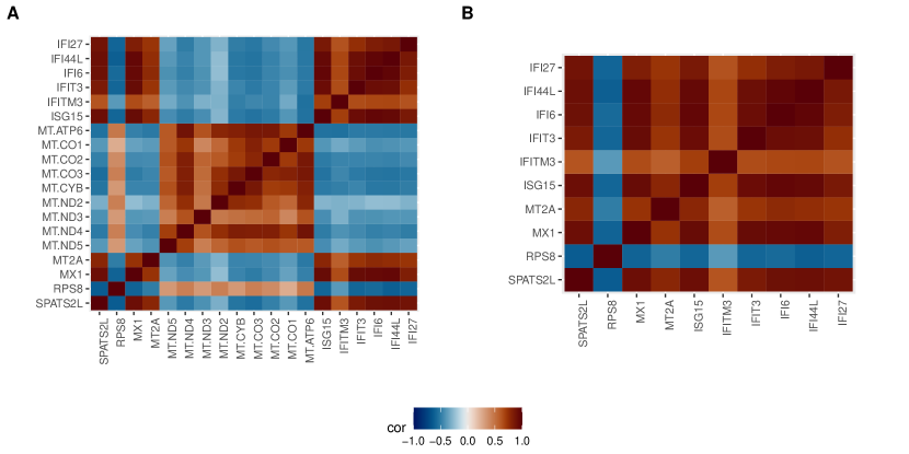
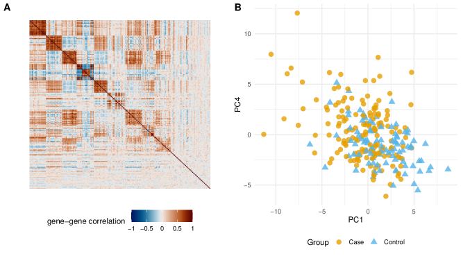
While interpretability is indispensable for scRNA data analysis, it usually comes under nontrivial assumptions about the signal and covariance structures. Simultaneous dimension reduction and variable selection can be achieved through sparse principal components analysis [sPCA 61, 24, 52], and has been applied in genetics study of schizophrenia [60]. In many biological settings, sparse factors are well justified. For example, a transcription factor regulates a set of genes with common features (motifs) creating a regulatory network [6]. Building on this idea, [27] argued that statistically derived factors often identify coordinated biological activity, which can be usefully modeled. In a related direction, a collection of methods termed “contrastive dimension reduction” [62, 1, 25] have been developed to identify systematic differences in covariance matrices between groups of genes. In the mean inference literature, a recent work [59] develops a Bayesian method under a low-dimensional sparse factor model and demonstrates how it can localize groups of genes that drive the difference between groups. These recent research trends reflect a consensus understanding that the gene expressions in a cell are co-regulated [43] and the number of correlation clusters is much smaller than the number of genes (Figure 1A). The genes in the same cluster—Figure 1 shows principle component (PC) genes clusters—are likely functioning in related pathways [16]. It is of great interest to determine whether the expression levels of these modules or factors are different between groups. In fact, one of the first few exploratory visualizations with a fresh scRNA-seq data set is a scatter plot of each sample’s principle component score (Figure 1B). In the presented Lupus data example (detailed in Section 6), we can observe a bimodal pattern in both the PC1 and PC4 directions, indicating the genes contained in these two PCs may have different expression levels and are worth further investigation. It is then natural to ask whether this visual bimodal pattern in these two directions is due to some genuine difference between the groups or due to randomness. One of the main objectives of this work is to provide a statistically principled answer to this question.
In single-cell sequencing data, each cell’s gene expression profile is represented as a -dimensional vector, where the ambient dimension typically ranges from to . Let the samples from the case and control groups be , and assume they are independent and identically distributed (IID) from two distributions . The global null hypothesis for the two-sample mean problem is
| (1) |
where are the population means of , respectively. While many statistical tests have been developed for the global null (1), to enhance the interpretability and power of the test, we consider the following projected null, which is inspired by the correlation structure in scRNA data (Figure 1):
| (2) |
where is a sparse vector. When the vector is known, the problem (2) is just a simple two-sample mean test and can be effectively solved using standard methods such as the student’s -test or the Wilcoxon’s rank-sum test. The vector provides both dimension reduction and, when is sparse, variable selection. In this case, rejecting the projected null not only asserts that and are different but also indicates that there is a significant difference in the subspace spanned by a few coordinates. However, in practice, such a vector must be estimated from the data. In the single-cell sequencing literature, it is plausible to assume that genes form clusters and coordinate with each other, and such gene clusters are likely to contribute to both the differential expression between two samples as well as the mode of variability [59]. In other words, one can expect the existence of a sparse vector supported on one or a few such clusters, such that it is aligned with both the difference vector and also explains much of the gene expression variability. This structural assumption points to a natural proxy of as the leading principle component vector of the gene expression.
The leading principal component direction of gene expression is unknown and must be estimated from the samples (the x-axis direction of Figure 1B is an example). Other leading PCs are also interesting projection directions. The orthogonality of PCs can further facilitate the exploration of systematic differential structures of the data in hand: we present only about of the total genes in Figure 1A and the correlation structure fades away quickly as the PC index increases, which also indicates a real-data covariance matrix can be well-approximated by some low-rank estimates based on PCs. In this paper, we introduce our method and theory focusing on the leading principle component, but extension to multiple PCs is straightforward and illustrated in our numerical examples.
Since the estimation of high dimensional sparse principal components has been extensively studied [see 61, 24, 52, for example], it is tempting to plug in an estimated principal component and treat it as fixed in the projected testing problem (2). However, the estimation error in the principal components may have non-negligible effects on subsequent inference, as the convergence rate is usually slower than . The first main contribution of this work is a detailed study of the effect of estimation error in the projection direction on the inference problem under different scenarios of the true parameter and the null hypothesis considered. We show that when , this estimation error does not affect the validity of the plug-in two-sample test, while it causes substantial bias if for the projected null (2), leading to biased confidence intervals for the effect size.
To correct the bias in the plug-in estimate, we implement a semiparametric one-step procedure [3, 49, 28, 8, 26, 17, 38] to construct an asymptotically normal estimate of the parameter . Such a one-step estimate involves the influence function of principal components, which are estimated using sparse PCA methods. To our knowledge, this is the first work combining sparse PCA with one-step estimation.
Our second methodological contribution is a more powerful test for the global null (1) assisted by a sparse projection. While choosing the projection to be the leading principal component can provide valid inference for the projected inference after debiasing, it may not provide the most power for testing the global null, especially when the mean difference is not substantially aligned with the leading principal components. This motivates us to look for a different, more adaptive sparse projection direction. A natural choice is the linear discriminating direction that best separates the two populations. In the high-dimensional inference literature, sparse discriminant analysis has been studied with appealing theoretical properties [4]. Again, as in the principal component projection, such a sparse projection vector must be estimated from the data and must be debiased. A major challenge in this approach is that under the global null hypothesis, such a linear discriminating direction is not well-defined and the influence function required in debiasing is degenerate. This is a common problem encountered in two-sample testing involving nuisance parameters [33, 56, 11, 35]. To tackle this challenge, we develop an “anchored projection” test, which adaptively combines the linear discriminating direction and the principal component. Under the alternative, the discriminating direction is well-defined and determines the projection direction. Under the null, the discriminating direction is insignificant and is overtaken by, or anchored at, the leading principal component, which is always well-defined and non-degenerate. We establish the validity of this test under standard high-dimensional inference contexts and demonstrate its strong performance through numerical examples.
Notation.
Our method uses the one-step estimation framework, which involves sample-splitting and cross-fitting, where we use a fraction of the data to estimate nuisance parameters such as PC vectors or discriminant directions, and the rest of the samples are used to construct the test statistics. Formally, we use to denote the sample from and the sample from . The integer denotes the number of folds of sample splitting. For ease of presentation, we assume are integers. When we say “data in the -th fold”, we are referring to the sub-sample
The complete data set is , and the samples not in split are denoted as . We also use .
For a matrix , we use to denote its Moore–Penrose pseudoinverse. For a positive-semidefinite matrix , denotes its -th largest eigenvalue. We will use for the common, population covariance matrix of and , and for its -th eigenvalue and eigenvector, assuming they are uniquely defined.
2 Simple Plug-in Tests
In two-sample testing under the context of genomics applications, including scRNA-seq, investigators are usually not only interested in rejecting the global null hypothesis but also want more information regarding how they are different. One commonly used strategy in the literature [31, 59, 20] is the plug-in projection, which can be summarized as follows.
-
1.
Given a large collection of genes and their gene-expression level measurements in two groups, estimate a direction vector that can summarize the variation pattern of the genes. One commonly considered direction in the literature is the estimated top PC vector. Denote this direction as .
-
2.
Calculate the difference between the sample average expression and , and project it onto the estimated gene group .
If the inner product’s magnitude significantly exceeds its plug-in standard error as if were non-random, people may claim that 1) there is a difference between the means; and 2) the difference is in a direction well-aligned with the PC direction. The general statistical validity of such claims is questionable since it does not factor in the variance of estimating . Moreover, due to the “double-dipping” of data—which refers to the fact that the same data is used to obtain and the inference of —a consistent estimator of is usually not enough, people typically need better convergence property to establish theoretical guarantees.
To start our investigation, we first de-couple the dependence between and estimates of PC1 by considering the plug-in statistic using a sample-splitting scheme:
| (3) |
Here is the first eigenvector of the population covariance matrix , and is the related plug-in test statistics. And , and the estimated mean vectors using samples in the -th split. The estimate of , , is calculated using . The variance estimator of is:
| (4) |
Remark 2.1.
In the above definition of , we implicitly assume the eigenvector is well-defined. That is, there is a unique eigenvector—up to sign flipping—that corresponds to the largest eigenvalue of the covariance matrix (its geometric multiplicity is ). We also assume the two samples have a common population covariance matrix. We can alternatively define as the top eigenvector of , which may actually be preferred in practice since they represent the gene correlation under in the control group (more natural status). Assuming a common covariance matrix can simplify our presentation. Mathematically, it is a slightly more complex case than “control-covariance” case, mainly due to a more intricate influence function form that involve both case and control samples (further elaborated in Section 3). Corresponding plug-in can also be calculated for other eigenvectors so long as they are well-defined.
Remark 2.2.
Since the leading PC is identifiable only up to a sign. We assume the signs of the estimates are aligned such that for all when constructing (3).
The simulated distribution of under both the global null and the projected null is presented in Figure 2. Under the global null, there is no difference between in any dimensions. For the projected null, we choose such that whereas . We can see the distribution of is close to standard normal under but overdispersed under . This implies may be used as a valid test statistic for the global null but should not be implemented when testing the more informative projected null—the variance estimator is not correct in the latter setting. This property is formally stated in Theorem 2.1. The details of the simulation are listed in Appendix A.
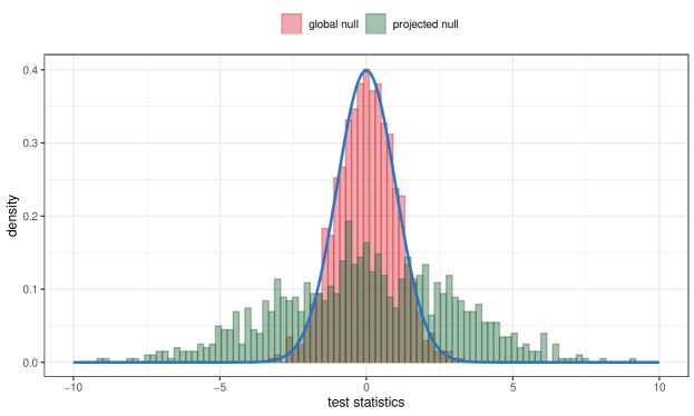
The empirical distribution under the global null in Figure 2 may seem surprising, as it is well-known that the leading PC cannot be estimated at rate in high dimensions unless the signal strength is unusually high, [23, 51, 53], and one would expect the estimation error in the nuisance parameter will lead to biased inference. However, the special structure of the test statistic will nullify the nuisance noise under the global null, making it irrelevant in the first order. This is a favorable property, meaning is a valid test statistic for .
Theorem 2.1.
Suppose is calculated from the IID samples and the split number is fixed. We further assume that
-
•
(S1) The projected variables of , on the population PC have non-zero variance: .
-
•
(S2) The common covariance matrix, , has a bounded largest eigenvalue . Moreover, there is a strictly positive gap between the first and second eigenvalues of : .
-
•
(S3) Each is a consistent estimator of : as . Similar conditions are also required for and .
Then under the global null hypothesis ,
| (5) |
as .
3 Debiased Tests for the Projected Null
In this section, we develop a method for testing the projected null hypothesis when is the top principle component of the population covariance matrix. The parameter of interest is
| (6) |
If we can establish an asymptotic normal estimator of , then we can use it to construct confidence intervals and derive a corresponding test for . As we observed in Section 2, the plug-in estimator is not asymptotically normal in general due to the error in the nuisance parameter estimates . To address this issue, we leverage the “one-step” correction technique to boost a slow-rate estimator of to an -asymptotically normal estimator.
We propose applying the following statistic to test the projected null :
| (7) |
where
| (8) |
Here is an estimate of the common covariance matrix using samples in , and is an estimate of . Similar to in (4), the quantity is a sample-splitting estimate of the standard deviation of . We present its explicit formula in Appendix C. When constructing , the mean vector estimators from -th split were simple sample averages and we will use the same choice for . However, the out-of-fold mean estimators , need not be simple averages. In fact, in the high-dimensional setting, soft-thresholding estimators of the means are known to have better theoretical properties under certain sparsity assumptions (which is also likely to hold in scRNA applications). See Remark 3.1.
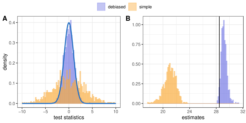
The distributions of and under the projected null—when but —are presented in Figure 3A. As we have seen earlier, the distribution of no longer approximates a standard normal. This implies should not be applied to test since their test size is not well-controlled. In contrast, the distribution of is close to , providing both validity and interpretability.
The estimate of in differs from by including a “one-step” correction, which corresponds to the influence function [36, 10] of with respect to the nuisance parameter . Such a one-step correction often leads to a -consistent, asymptotically normal estimate. The difference between and when estimating a is illustrated in Figure 3B.
We formally state the aforementioned distributional results as follows.
Theorem 3.1.
Suppose is calculated from an IID sample and the split number is fixed. In addition to assumptions (S1)- (S3) in Theorem 2.1, we further assume that
-
•
(D1) The difference between the population means is bounded by a constant.
-
•
(D2) are all of order , where denotes the spectral norm for a matrix.
-
•
(D3) as . A similar condition also holds for .
Then under the projected null hypothesis we have,
| (9) |
as .
Remark 3.1.
Compared with Theorem 2.1, condition (D2) in Theorem 3.1 is the most essential extra requirement regarding nuisance parameter estimation. It requires the high-dimensional quantities , to be estimated at a rate faster than (recall in low-dimensional settings they can be estimated in a parametric rate ). This type of condition is common in the one-step estimation literature—-including the well-known doubly-robust estimator of average treatment effect [15]. When diverges faster than , the above rate no longer satisfies our requirement (D2).
In our case, we can apply some regularized estimators of to achieve the rate. One choice is simply calculating simple sample means from and hard threshold each entry at . This procedure and a close variation (“soft-thresholding”) give estimators converging in rate , assuming a finite number of entries of has non-zero population means [22]. In statistical literature, this type of estimator has been extensively discussed in wavelet nonparametric regression in the 1990s [13]. It is also related to James-Stein estimator [40] and Lasso under orthonormal designs ([47], Section 10).
Estimation of high-dimensional covariance matrices is a more recent topic and has been extensively studied in the past two decades. The high dimensionality is often tackled by some covariance structures such as low-rank, approximate block-diagonal, or sparsity. The theoretical rates of many estimators, measured in the operator spectral norm , are often of order or with some regularity index , possibly achieving the required rate in (D2). We refer our readers to [14, 5, 29] for more extensive surveys of frequently imposed structures and available methods.
Remark 3.2.
Condition (D2) may imply condition (D3) under certain boundedness conditions on the components of (convergence in probability does not unconditionally imply convergence in moments). Since they are neither sufficient nor necessary for each other and control different elements in the proof, we state them separately. For semi-parametric estimation without sample-splitting, condition (D3) needs to be modified to a stronger version restricting the estimates in a Donsker class (e.g. [26] Section 4.2).
4 Anchored Projection Tests for the Global Null
While the PCA debiased projection procedure developed in the previous section provides valid inference under the projected null hypothesis, it may not provide full power against the global null hypothesis when the mean difference is not well-aligned with the leading PCs. Depending on the scientific research goal, one may alternatively be interested in interpretable tests that prioritize power over the correlation structure. Following the sparse projection idea, it is then natural to project the difference vector in a sparse direction that best separates the two populations.
Constructing high-dimensional sparse linear classifiers has been well-studied in the literature, including logistic Lasso [47, 50] and sparse LDA [39, 4]. However, under the global null, this discriminating direction becomes degenerative. In practice, it is also direct to verify via a simple simulated experiment (Figure E.7) that cross-validated linear classifiers such as logistic Lasso have a positive probability to be exactly zero. This is a common challenge faced by two-sample tests under the global null hypothesis, and most existing results [33] are only established under the alternative hypothesis.
In order to overcome the degeneracy issue, we propose a hybrid sparse projection that adaptively “anchors” the potentially degenerative discriminating direction to a sparse PC vector when the signal is weak. When the signal is moderately strong, the hybrid projection direction will mainly follow the discriminating direction, which yields higher power. On the other hand, when the signal is weak, the estimated discriminating direction is noisy and the sparse PC takes over to avoid degeneracy.
Let be a discriminating direction estimated from all data except the th fold. Our adaptive anchored projection test statistic has the following form:
| (10) |
The normalizing standard error is similarly defined as in (4), replacing by the hybrid projection vector , normalized to have unit -norm. The weight parameter diverges as is a hyperparameter of the method, which shifts the projection direction towards when the signal is strong. Under , the component will dominate so long as does not diverge too fast, avoiding degeneracy and allowing for tractable distribution of .
Corollary 4.1.
Suppose is calculated from an IID sample and the split number is fixed. In addition to the assumptions (S1)-(S3) in Theorem 2.1, we further assume that
-
•
(ANC) .
Then under the global null hypothesis we have:
| (11) |
as .
The proof of Corollary 4.1 is direct after establishing Theorem 2.1, details presented in Appendix F.
Remark 4.1.
(Power of the anchored test) The discriminating direction can be related to the distributions of and through a classification problem, where we associate each sample point in the pooled data a binary label , according to whether this sample comes from the population or the population. Then it is natural to define as the best linear discriminating direction or the logistic regression coefficient, which can be estimated using the corresponding high-dimensional sparse estimators [50, 4]. In either choice, it is direct to check that when the true discriminant direction is zero, the class label is independent of the data vector, which further implies the global null hypothesis . Therefore, the test based on the anchored projection statistic has power converging to , so long as and .
Remark 4.2.
The choice of discriminating direction estimate can be quite flexible, and there are many proposals in the literature such as sparse logistic regression [50] and sparse linear discriminant analysis [4]. In practice, we also found a thresholded-version of works well: for some threshold level . This allows us to use a large so that converges to much faster when the signal surpasses the threshold.
The theoretical choice of the threshold depends on the rate of convergence of the original estimate . When the true regression coefficient is zero, in typical high-dimensional sparse classification settings we usually have , so that the anchoring test statistic will offer asymptotically valid null distribution as long as . In our numerical examples, the choice of has worked reasonably well. With this the choice of becomes less sensitive and we use in both simulation and real-data analysis. We will proceed with this choice of in the rest of the paper—coupled with Logistic Lasso estimates . If one replaces the (ANC) condition with , the related is also asymptotically normal under the global null hypothesis, using a similar argument as Corollary 4.1. When , the shrinkage function reduces to an identity mapping (10). In this case we can usually take for some .
5 Simulation Studies
In this section, we present some numerical results based on simulated data sets. We are interested in the performance of , and (with logistic Lasso) as well as a literature method for comparison [7]. The existing method is a popular, powerful procedure for testing the global null and is more favored over other existing methods when there are small signals in most dimensions (the -type alternative in [19]). The authors also applied their method to some gene-set comparison problems. All of the methods discussed in this work, including and are included in R package HMC—available on the Comprehensive R Archive Network (CRAN).
In this work, we simulate data under three scenarios: the global null ; a “strictly weaker” projected null , with but ; and the alternative hypothesis , . That is, in the alternative hypothesis setting, there are signals that align with both population PC1 and PC2. In this section, we will focus on the validity and power of the tests. Interpretability will be explored in the real-data example. We reject the null hypothesis when the absolute value of the test statistics is greater than -quantile of . Under , we expect the three discussed statistics to have an approximate rejection proportion. For , only is expected to have a -size, while the other two have an inflated rejection rate because they are designed for . Under the alternative hypothesis, we prefer a test that rejects more often, illustrating better power.
We consider a “zero-inflated normal” distribution of and . The sample matrix would have a significant proportion of exact zeros, mimicking normalized scRNA data where gene expression reads are highly sparse. We use equal sample sizes for both groups, selected from . Sample dimension . The samples have a sparse, spiked covariance structure [21]. See Appendix G for a complete description of simulation details.
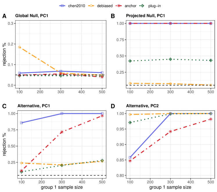
The rejection proportion of each test in different settings is estimated with Monte Carlo repeats and the results are presented in Figure 4. Under the global null when there is absolutely no signal (Figure 4, A), all of the methods have well-calibrated rejection proportion when sample sizes are greater than . The debiased test statistics has an inflated type I error when the sample size is small.
Under the projected null, meets the expected rejection proportion with larger sample sizes (Figure 4, B). Although the difference is orthogonal to , the absolute norm of the difference is set to be large, which makes and the literature method always reject. The plug-in statistic also shows some “power”, but this implies it cannot be used as a valid test for although formally it is tempting to apply it to this case.
The results in Figure 4, C & D correspond to the same simulation setting (alternative hypothesis), but the implemented comparison methods are different. We consider , and that target/anchor at PC1 in subplot C, whereas in panel D it is their PC2-version being assessed. The literature method is identical across the two subplots. The signal aligned with PC1 is set to be smaller than that with PC2 , therefore the observed rejection rate is, in general, lower in panel C than D. The method can leverage the signal from both and and appear to be more powerful than the PC1 versions (but less than PC2 versions). Notably, the anchored-test can adaptively adjust the projection direction to where the stronger signal lies, even when it is anchored to the sub-optimal direction (Figure 4 C).
6 An Application to Immune Cell Gene Expression in a Lupus Study
6.1 Data Set and Pre-processing
The proposed procedures and are applied to analyze a large study of single-cell differential expression in an immune-related disease [37]. In this data set, the authors used scRNA-sequencing to study the molecular mechanisms of Systemic Lupus Erythematosus (SLE), which is a heterogeneous autoimmune disease with elevated prevalence in women and individuals of Asian, African, and Hispanic ancestry. One of the goals of this study is to assess the differentially expressed genes in various types of immune cells between the SLE case and control groups. The public data set contains the expression profile information of million cells from 8 major cell types and individuals— of them have SLE and are healthy. We use the Python package scanpy [57] to pre-process the single-cell data and select the top highly variable genes within each cell type. For each cell type, we aggregate expression across cells from the same individual to obtain “pseudo-bulk” counts for each gene, and then remove genes expressed in less than 10 individuals. This means each sample of our analysis corresponds to one individual and they can be treated as IID samples from several homogeneous populations. Next, we applied the standard log-normalization (e.g. equation (1) in [25]), converting raw expression count to its logarithm, to stabilize the sample value and make it more amenable to comparisons. In this study, we focus on important immune cell types with a moderately large number of samples and compare the case and control gene-expression profiling within each. We also regress out the library size, sex, population, and processing cohorts to remove potential confounding. The gene expression variable (i.e. each dimension of ) is normalized to unit-variance. We use split sample-splitting scheme when performing our tests.
6.2 Testing Results
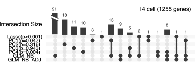
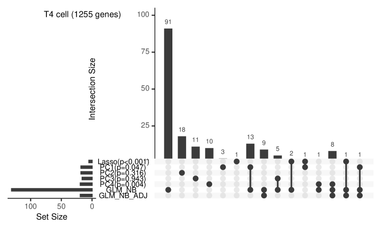
The anchored-Lasso test and the debiased test for the top four PC directions are applied to the CD4 T lymphocytes (T4), a critical cell type that helps to coordinate the immune response (Figure 5, results for other cell types are presented in Appendix H). For , the reported p-value corresponds to the global null, whereas the debiased tests , , correspond to the projected nulls , , respectively. The anchored test and the PC1, PC4 debiased tests report significant differences at the standard threshold. The latter two results answer our motivating questions in the Introduction (Figure 1B): the observed distributional difference between case and control samples, in the directions of PC1 and PC4, is indeed statistically significant.
Further details regarding the systematic signal are displayed in Figure 5 and 6. The PCs define the “active genes”, which are defined as those genes consistently (across different data splits) taking non-zero loadings in or : specifically, we define a gene to be active if it takes non-zero loadings in more than half of the estimated high-dimensional sparse vectors (“majority voting”). Assessing how much the non-zero genes vary between splits can also offer researchers basic intuition regarding the noise level when estimating .
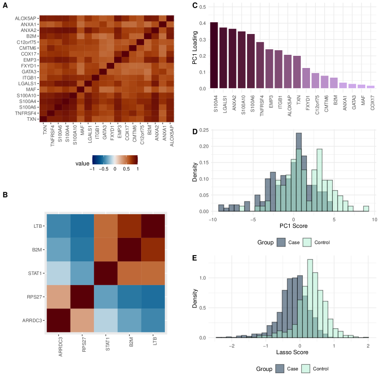
The number of active genes for each of the PC1-PC4 is approximately (Figure 5). PC1 () includes genes and of them are reported to be marginally significant according to a standard univariate negative-binomial regression (p-value threshold ); however, only one survives adjustment for multiple comparisons. A further inspection of the PC1 active genes and the estimated is provided in Figure 6 A, C. These genes are all highly correlated and likely have similar functions in the immune system. PC4 () includes 19 genes and of them are reported marginally significant according to the marginal tests (-level) and 8 retain significance after multiple comparison corrections. We provide the gene names and their correlation in Figure H.12. In panel A, we can observe the genes are divided into two association blocks: One contains all the mitochondrial genes, which are not protein-coding genes. These genes are not well studied in the literature and are often removed from such analyses. The other block contains multiple genes having significant functions in the immune system: as many of their names suggest, the ”IFI” prefix stands for ”InterFeron-Inducible,” indicating that these genes are up-regulated in response to interferon signaling, which is an anti-virus mechanism in the human body.
The anchored-Lasso solution is more parsimonious than the PC methods, identifying 5 active genes (Figure 5). Among the 5, one (B2M) overlaps with the estimated PC1 vector, and the rest are not included in the leading PCs. As illustrated by the sample correlation between these genes (Figure 6B), they are not highly correlated. Using this small set of signal genes, we can effectively separate the case and control individuals (Figure 6E). Compared with the discrimination capacity of PC1 (Figure 6D), Lasso’s score distribution is visually more bimodal, which is expected as we selected these genes via a label-prediction task. Among the five active genes, four (except for RPS27) are reported in the biomedical literature to encode important proteins in immune response and/or antiviral activity[9, 46, 32, 44]. Depending on the specific purpose of the scientific research, a user can decide which test is more relevant to each of their goals. Regardless, our methods will likely point them to more biologically meaningful signals than a simple global test.
7 Discussion
In this paper, we studied three projection-based high-dimensional mean comparison procedures. The sparse projection-based tests offer better interpretability and take advantage of the interaction between the signal features. The PC-projection test aims to find the difference aligned with the leading principal components and requires debiasing in order to provide valid inference for the effect size in the presence of a high-dimensional nuisance parameter. The anchoring procedure offers higher power when the difference is not fully contained in the PC subspace. In practice, this type of test can often offer a short list of relevant features to the users for follow-up investigations. In contrast to the univariate multiple comparison approaches [12], our projection-based method handles dependence more naturally and accurately, and guarantees family-wise error rate control without requiring multiple comparison correction.
The asymptotic results for the plug-in test presented in Section 2 can be extended to other cases. In our derivation, the estimation error in is nullified by the zero difference . The essential requirement is for to be a consistent (at any rate) estimator of a well-defined . There is nothing special about being the principal component, and Theorem 2.1 can be directly generalized to cover a broader category of projection-based tests. We present the following Proposition as a generalization to Theorem 2.1.
Proposition 7.1.
Let be a fixed unit vector and denote our sample-splitting estimates of it as , (similar to ). Define test-statistic similarly to . Suppose is calculated from the IID samples and the split number is fixed. We further assume that conditions (S1), (S3) hold similarly for and . Moreover, we require
| (12) |
Then as .
The proof of Proposition 7.1 is presented in Appendix B, which is almost identical to that of Theorem 2.1. This result does not require to be the principle component vector of any matrix and permits implementing any consistent estimators of it.
We state a set of achievable and practically relevant sufficient conditions for (12). Given a marker gene that is of research interest, define vector to be the PC1 vector of a submatrix of , only containing genes correlated with . Let be an high-dimensional sparse vector padding all the other dimensions of with . Such a is referred to as the “eigengene” in biomedical literature (e.g.[30], equation (29)) and can be used as a clinical covariate. A researcher may be interested in whether differential expression exists for this “correlation module” between their treatment and control groups, formulated as for all . Typically, researchers do not have a priori knowledge of which genes are associated with gene in their specific setting. We claim that so long as with probability , meaning our estimate does not mistakenly include any genes independent from G, the condition (12) is satisfied and is asymptotically normal. This is plausible given a light tail of (logarithm-transformed) gene expression counts via a -scale truncation. When we observe large , it means that at least one gene in this correlation module is differentially expressed. This problem and variations on this theme have been studied in biomedical research using methods like WGCNA [31] during the past decade. The above procedure is also applicable when there is no pre-specified gene , and it can be applied to each correlation block discovered from samples. Proposition 7.1 provides a theoretically justifiable procedure to assess the validity of such discoveries.
Acknowledgments
We appreciate Jin-Hong Du’s assistance in preparing the data presented in Section 6. This project was funded by National Institute of Mental Health (NIMH) grant R01MH123184 and NSF DMS-2015492.
References
- Abid et al. [2018] Abid, A., M. J. Zhang, V. K. Bagaria, and J. Zou (2018). Exploring patterns enriched in a dataset with contrastive principal component analysis. Nature communications 9(1), 2134.
- Bai and Saranadasa [1996] Bai, Z. and H. Saranadasa (1996). Effect of high dimension: by an example of a two sample problem. Statistica Sinica, 311–329.
- Bickel et al. [1993] Bickel, P. J., C. A. Klaassen, P. J. Bickel, Y. Ritov, J. Klaassen, J. A. Wellner, and Y. Ritov (1993). Efficient and adaptive estimation for semiparametric models, Volume 4. Springer.
- Cai and Liu [2011] Cai, T. and W. Liu (2011). A direct estimation approach to sparse linear discriminant analysis. Journal of the American statistical association 106(496), 1566–1577.
- Cai et al. [2016] Cai, T. T., Z. Ren, and H. H. Zhou (2016). Estimating structured high-dimensional covariance and precision matrices: Optimal rates and adaptive estimation. Electronic Journal of Statistics 10(1), 1 – 59.
- Carvalho et al. [2008] Carvalho, C. M., J. Chang, J. E. Lucas, J. R. Nevins, Q. Wang, and M. West (2008, Dec). High-dimensional sparse factor modeling: Applications in gene expression genomics. J Am Stat Assoc 103(484), 1438–1456.
- Chen and Qin [2010] Chen, S. X. and Y.-L. Qin (2010). A two-sample test for high-dimensional data with applications to gene-set testing. The Annals of Statistics 38(2), 808 – 835.
- Chernozhukov et al. [2018] Chernozhukov, V., D. Chetverikov, M. Demirer, E. Duflo, C. Hansen, W. Newey, and J. Robins (2018, 01). Double/debiased machine learning for treatment and structural parameters. The Econometrics Journal 21(1), C1–C68.
- Creus et al. [2012] Creus, K. K., B. De Paepe, J. Weis, and J. L. De Bleecker (2012). The multifaceted character of lymphotoxin in inflammatory myopathies and muscular dystrophies. Neuromuscular Disorders 22(8), 712–719.
- Critchley [1985] Critchley, F. (1985). Influence in principal components analysis. Biometrika 72(3), 627–636.
- Dai et al. [2022] Dai, B., X. Shen, and W. Pan (2022). Significance tests of feature relevance for a black-box learner. IEEE Transactions on Neural Networks and Learning Systems.
- Das et al. [2021] Das, S., A. Rai, M. L. Merchant, M. C. Cave, and S. N. Rai (2021). A comprehensive survey of statistical approaches for differential expression analysis in single-cell rna sequencing studies. Genes 12(12), 1947.
- Donoho [1995] Donoho, D. L. (1995). De-noising by soft-thresholding. IEEE transactions on information theory 41(3), 613–627.
- Fan et al. [2016] Fan, J., Y. Liao, and H. Liu (2016). An overview of the estimation of large covariance and precision matrices. The Econometrics Journal 19(1), C1–C32.
- Glynn and Quinn [2010] Glynn, A. N. and K. M. Quinn (2010). An introduction to the augmented inverse propensity weighted estimator. Political analysis 18(1), 36–56.
- Hastie et al. [2000] Hastie, T., R. Tibshirani, M. B. Eisen, A. Alizadeh, R. Levy, L. Staudt, W. C. Chan, D. Botstein, and P. Brown (2000). ’gene shaving’as a method for identifying distinct sets of genes with similar expression patterns. Genome biology 1(2), 1–21.
- Hines et al. [2022] Hines, O., O. Dukes, K. Diaz-Ordaz, and S. Vansteelandt (2022). Demystifying statistical learning based on efficient influence functions. The American Statistician 76(3), 292–304.
- Hotelling [1931] Hotelling, H. (1931). The Generalization of Student’s Ratio. The Annals of Mathematical Statistics 2(3), 360 – 378.
- Huang et al. [2022] Huang, Y., C. Li, R. Li, and S. Yang (2022). An overview of tests on high-dimensional means. Journal of multivariate analysis 188, 104813.
- Jin et al. [2020] Jin, X., S. K. Simmons, A. Guo, A. S. Shetty, M. Ko, L. Nguyen, V. Jokhi, E. Robinson, P. Oyler, N. Curry, et al. (2020). In vivo perturb-seq reveals neuronal and glial abnormalities associated with autism risk genes. Science 370(6520), eaaz6063.
- Johnstone [2001] Johnstone, I. M. (2001). On the distribution of the largest eigenvalue in principal components analysis. The Annals of statistics 29(2), 295–327.
- Johnstone [2019] Johnstone, I. M. (2019). Gaussian estimation: Sequence and wavelet models. Unpublished Book.
- Johnstone and Lu [2009] Johnstone, I. M. and A. Y. Lu (2009). On consistency and sparsity for principal components analysis in high dimensions. Journal of the American Statistical Association 104(486), 682–693.
- Jolliffe et al. [2003] Jolliffe, I. T., N. T. Trendafilov, and M. Uddin (2003). A modified principal component technique based on the lasso. Journal of Computational and Graphical Statistics 12, 531–547.
- Jones et al. [2022] Jones, A., F. W. Townes, D. Li, and B. E. Engelhardt (2022). Contrastive latent variable modeling with application to case-control sequencing experiments. The Annals of Applied Statistics 16(3), 1268–1291.
- Kennedy [2022] Kennedy, E. H. (2022). Semiparametric doubly robust targeted double machine learning: a review. arXiv preprint arXiv:2203.06469.
- Knowles and Ghahramani [2011] Knowles, D. and Z. Ghahramani (2011). Nonparametric Bayesian sparse factor models with application to gene expression modeling. The Annals of Applied Statistics 5(2B), 1534 – 1552.
- Kosorok [2008] Kosorok, M. R. (2008). Introduction to empirical processes and semiparametric inference, Volume 61. Springer.
- Lam [2020] Lam, C. (2020). High-dimensional covariance matrix estimation. Wiley Interdisciplinary reviews: computational statistics 12(2), e1485.
- Langfelder and Horvath [2007] Langfelder, P. and S. Horvath (2007). Eigengene networks for studying the relationships between co-expression modules. BMC systems biology 1, 1–17.
- Langfelder and Horvath [2008] Langfelder, P. and S. Horvath (2008). Wgcna: an r package for weighted correlation network analysis. BMC bioinformatics 9(1), 1–13.
- Largent et al. [2023] Largent, A. D., K. Lambert, K. Chiang, N. Shumlak, D. Liggitt, M. Oukka, T. R. Torgerson, J. H. Buckner, E. J. Allenspach, D. J. Rawlings, et al. (2023). Dysregulated ifn- signals promote autoimmunity in stat1 gain-of-function syndrome. Science Translational Medicine 15(703), eade7028.
- Liu et al. [2022] Liu, W., X. Yu, and R. Li (2022). Multiple-splitting projection test for high-dimensional mean vectors. The Journal of Machine Learning Research 23(1), 3091–3117.
- Lucas et al. [2010] Lucas, J. E., H.-N. Kung, and J.-T. A. Chi (2010, Sep). Latent factor analysis to discover pathway-associated putative segmental aneuploidies in human cancers. PLoS Comput Biol 6(9), e1000920.
- Lundborg et al. [2022] Lundborg, A. R., I. Kim, R. D. Shah, and R. J. Samworth (2022). The projected covariance measure for assumption-lean variable significance testing. arXiv preprint arXiv:2211.02039.
- Magnus [1985] Magnus, J. R. (1985). On differentiating eigenvalues and eigenvectors. Econometric theory 1(2), 179–191.
- Perez et al. [2022] Perez, R. K., M. G. Gordon, M. Subramaniam, M. C. Kim, G. C. Hartoularos, S. Targ, Y. Sun, A. Ogorodnikov, R. Bueno, A. Lu, et al. (2022). Single-cell rna-seq reveals cell type–specific molecular and genetic associations to lupus. Science 376(6589), eabf1970.
- Rakshit et al. [2023] Rakshit, P., Z. Wang, T. T. Cai, and Z. Guo (2023). Sihr: Statistical inference in high-dimensional linear and logistic regression models.
- Shao et al. [2011] Shao, J., Y. Wang, X. Deng, and S. Wang (2011). Sparse linear discriminant analysis by thresholding for high dimensional data. The Annals of Statistics 39(2), 1241 – 1265.
- Stein [1956] Stein, C. (1956). Inadmissibility of the usual estimator for the mean of a multivariate normal distribution. In Proceedings of the Third Berkeley Symposium on Mathematical Statistics and Probability, Volume 1: Contributions to the Theory of Statistics, Volume 3, pp. 197–207. University of California Press.
- Stein-O’Brien et al. [2018] Stein-O’Brien, G. L., R. Arora, A. C. Culhane, A. V. Favorov, L. X. Garmire, C. S. Greene, L. A. Goff, Y. Li, A. Ngom, M. F. Ochs, Y. Xu, and E. J. Fertig (2018, Oct). Enter the matrix: Factorization uncovers knowledge from omics. Trends Genet 34(10), 790–805.
- Stewart [1977] Stewart, G. W. (1977). On the perturbation of pseudo-inverses, projections and linear least squares problems. SIAM review 19(4), 634–662.
- Stuart et al. [2003] Stuart, J. M., E. Segal, D. Koller, and S. K. Kim (2003). A gene-coexpression network for global discovery of conserved genetic modules. science 302(5643), 249–255.
- Takeuchi et al. [2019] Takeuchi, F., I. Kukimoto, Z. Li, S. Li, N. Li, Z. Hu, A. Takahashi, S. Inoue, S. Yokoi, J. Chen, et al. (2019). Genome-wide association study of cervical cancer suggests a role for arrdc3 gene in human papillomavirus infection. Human molecular genetics 28(2), 341–348.
- Tang et al. [2009] Tang, F., C. Barbacioru, Y. Wang, E. Nordman, C. Lee, N. Xu, X. Wang, J. Bodeau, B. B. Tuch, A. Siddiqui, et al. (2009). mrna-seq whole-transcriptome analysis of a single cell. Nature methods 6(5), 377–382.
- Tang et al. [2021] Tang, F., Y.-H. Zhao, Q. Zhang, W. Wei, S.-F. Tian, C. Li, J. Yao, Z.-F. Wang, and Z.-Q. Li (2021). Impact of beta-2 microglobulin expression on the survival of glioma patients via modulating the tumor immune microenvironment. CNS Neuroscience & Therapeutics 27(8), 951–962.
- Tibshirani [1996] Tibshirani, R. (1996). Regression shrinkage and selection via the lasso. Journal of the Royal Statistical Society Series B: Statistical Methodology 58(1), 267–288.
- Tony Cai et al. [2014] Tony Cai, T., W. Liu, and Y. Xia (2014). Two-sample test of high dimensional means under dependence. Journal of the Royal Statistical Society Series B: Statistical Methodology 76(2), 349–372.
- Tsiatis [2006] Tsiatis, A. A. (2006). Semiparametric theory and missing data.
- van de Geer [2008] van de Geer, S. A. (2008). High-dimensional generalized linear models and the lasso. The Annals of Statistics 36(2), 614–645.
- Vu and Lei [2012] Vu, V. and J. Lei (2012). Minimax rates of estimation for sparse pca in high dimensions. In Artificial intelligence and statistics, pp. 1278–1286. PMLR.
- Vu et al. [2013] Vu, V. Q., J. Cho, J. Lei, and K. Rohe (2013). Fantope projection and selection: a near-optimal convex relaxation of sparse PCA. In Advances in Neural Information Processing Systems 26.
- Vu and Lei [2013] Vu, V. Q. and J. Lei (2013). Minimax sparse principal subspace estimation in high dimensions. The Annals of Statistics 41(6), 2905–2947.
- Wainwright [2019] Wainwright, M. J. (2019). High-dimensional statistics: A non-asymptotic viewpoint, Volume 48. Cambridge university press.
- Wedin [1973] Wedin, P.-Å. (1973). Perturbation theory for pseudo-inverses. BIT Numerical Mathematics 13, 217–232.
- Williamson et al. [2023] Williamson, B. D., P. B. Gilbert, N. R. Simon, and M. Carone (2023). A general framework for inference on algorithm-agnostic variable importance. Journal of the American Statistical Association 118(543), 1645–1658.
- Wolf et al. [2018] Wolf, F. A., P. Angerer, and F. J. Theis (2018). Scanpy: large-scale single-cell gene expression data analysis. Genome biology 19, 1–5.
- Yu et al. [2015] Yu, Y., T. Wang, and R. J. Samworth (2015). A useful variant of the davis–kahan theorem for statisticians. Biometrika 102(2), 315–323.
- Zhou et al. [2023] Zhou, Y., K. Luo, L. Liang, M. Chen, and X. He (2023). A new bayesian factor analysis method improves detection of genes and biological processes affected by perturbations in single-cell crispr screening. Nature Methods.
- Zhu et al. [2017] Zhu, L., J. Lei, B. Devlin, and K. Roeder (2017). Testing high-dimensional covariance matrices, with application to detecting schizophrenia risk genes. The annals of applied statistics 11(3), 1810–1831.
- Zou et al. [2006] Zou, H., T. Hastie, and R. Tibshirani (2006). Sparse principal component analysis. Journal of computational and graphical statistics 15(2), 265–286.
- Zou et al. [2013] Zou, J. Y., D. J. Hsu, D. C. Parkes, and R. P. Adams (2013). Contrastive learning using spectral methods. Advances in Neural Information Processing Systems 26.
Appendix A Details of Figure 2
The distribution of under the global and projected nulls is presented in Figure 2. Here we present the details of the simulation settings.
The two-group samples are IID multivariate normal with equal covariance matrix. We used a two-split crossing fitting (). Number of samples in each split: , . Dimension of : . The mean of is
| (13) |
And that of is
| (14) |
The covariance matrices of are:
| (15) |
where is -dimensional identity matrix. The top PC vector is:
| (16) |
Note that we normalized such that .
For this, we implement standard PCA to estimate . We are aware that standard PCA is not a consistent estimator of in the high-dimensional setting but still stick to this choice because standard PCA is still routinely applied in high-dimensional biomedical research. Statistically, it is not the best practice but in this specific simulation, the estimation quality is satisfactory. Results do not significantly change after switching to sparse PCA.
Appendix B Proof of Theorem 2.1 & Proposition 7.1
Proof.
(Proof of Theorem 2.1) For the simplicity of exposition, we omit the subscript of and and denote them as and —also implying an identical argument also holds for other top eigenvectors. We first clean up the plug-in term related to group 1 data:
| (17) | ||||
Applying the same decomposition for group 2 data and take the difference:
| (18) | ||||
The first two terms in (18) are two independent random variables and each one of them converges to a normal distribution when properly normalized. The third term is zero under the global null hypothesis (but not zero under the projected null!). The last two terms are higher-order smaller, , as long as the conditions of Theorem 2.1 hold, which we will show later.
Continue (18), after aggregating the estimation from each splits we have:
| (19) |
which is essentially a sum of independent random variables (omitting the higher order terms). To apply Lindeberg’s central limit theorem, we need to normalize it by a consistent estimate of its standard deviation:
| (20) |
The cross-fitting variance estimator we used in (4) is one of the natural choices that do not require significant extra computation. It is a consistent estimator of (B) as by the law of large number. So we can establish the asymptotic normality of after applying Slutsky’s theorem. We also note that the Lindeberg’s condition is satisfied since both and have finite variances.
Now we show the last two terms in (18) are of higher order. Under the global null that , we just need to bound
| (21) |
For any :
| (22) | ||||
Using the independence between samples, the conditional variance can be handled as following:
| (23) | ||||
where are the covariance matrices of and (assumed to be identical in the main text). Here we used to denote the largest eigenvalue of a matrix. Plug (23) into (22),
| (24) | ||||
When converges to zero as , we know for any ,
| (25) |
∎
Proof.
(Proof of Proposition 7.1) Similar to the proof of Theorem 2.1, we have the following decomposition:
| (26) | ||||
In step , we apply the condition (Orth). In the proof of Theorem 2.1 we used , which is stronger than what we actually needed. The rest of the proof follows line-by-line to that of Theorem 2.1, replacing all the by . The asymptotic distribution of is identical to that of , the rest two terms are of higher order . ∎
Appendix C Explicit Formulas for the Debiased Test
We omitted presenting the explicit formula of several quantities for constructing in the main text to save some space. We present them in this section.
For simplicity of notation, we use to denote “taking empirical averaging with ”. For example,
| (27) |
The population-level influence functions, and , of the eigenvector functional are:
| (28) | ||||
The asymptotic variance estimator in is
| (29) |
where
| (30) | ||||
Appendix D Proof of Theorem 3.1
In this section we present the proof of the distribution of Theorem 3.1. We need to decompose the debiased test statistics into a sum of the central limit theorem terms, the empirical process “cross terms” and the (Taylor expansion) “remainder terms”. The latter two are of higher order and do not impact the distribution of the quantity of interest asymptotically (shown in Lemma D.1 and D.2). For simplicity of notation, we will drop the subscript of and . We will use to denote “taking empirical average with respect to data ”. We also use to denote taking expectation with respect to the underlying distribution , conditioned on . For example,
Define
To clarify, the notation means
Proof.
(Proof of Theorem 3.1) For each one of the splits, we will decompose its debiased estimate of into the aforementioned three terms and analyze them separately. The following step is merely algebraic, not requiring any additional assumptions:
| (31) | ||||
The first term in (31) is the main term that converges to a normal distribution, we will analyze its behavior soon. The vanishing latter two terms are handled in Lemma D.1 and D.2.
The summation of the estimate over splits can be written as:
| (32) | ||||
Note the influence function is mean-zero at the true distribution .
Similar to the proof of Theorem 2.1, we also need to normalize the summation in (32) to apply Lindeberg’s central limit theorem. The variance of the main terms in (32) is
| (33) | ||||
Our proposal (29) used a consistent estimator of . The testing statistics
Note that diverges no faster than . ∎
Lemma D.1.
Under the assumptions of Theorem 3.1. The “cross-term”
| (34) |
Proof.
We first split into two parts: a the inner product term and a term involving the influence function :
| (35) | ||||
The first inner product term above is just:
| (36) | ||||
which has been shown to be (specifically, in (23) in the proof of Theorem 2.1). We needed to consistently estimate and the covariance matrix of and has a bounded largest eigenvalue.
For the influence function terms, a similar argument also holds. We split the influence function into parts related to and respectively and bound them separately.
| (37) | ||||
Consider the parts involving :
| (38) | ||||
| (39) |
where is the difference between the estimated function and the truth.
Applying Chebyshev’s inequality:
| (40) | ||||
Given the assumption that
| (41) |
we know is . A similar argument also holds for the term associated with in (37). This implies their summation is also of order . ∎
Lemma D.2.
Proof.
We split the remainder into several terms that we will bound separately. Recall the notation :
| (44) | ||||
For the third term in the last line of (44) we have:
| (45) | ||||
In step we used the explicit form of (3) and —therefore it is the population mean-difference that dominates. In step we applied the assumed bounded mean-difference condition (D1) and that is bounded (with probability converging to ). Recall that in condition (S2) we assumed the eigen-gap . We will establish the latter in Lemma D.3. Similarly, the forth term in (44) can be bounded as:
| (46) |
In the rest of the proof, we are going to show the sum of the first two terms in (44) are “small”, leveraging that influence function is the first order derivative of the functional of interest. Let . Define an interpolation matrix between the estimated covariance matrix and the population one:
| (47) |
And define the eigenvector mapping as
| (48) |
We can see that and . Since the and are eigenvectors of a matrix at the same time, we further require for all to make this mapping well-defined. Similarly, we define the mapping that returns the largest eigenvalue of matrix .
Therefore
| (49) | ||||
In step and we use the derivative of exists and plug in its explicit form [36, 10]. Noting that and , we multiply both sides of (49) by , we have:
Go back to the first two terms in the last line of (44):
| (50) | ||||
Under our assumptions, the products above
| (51) | ||||
are all of order . We present the details of the argument in Lemma D.3. Combine this result with (45) and (46), we conclude our proof. ∎
In the following lemma, we show the remainder terms are small under the conditions listed in the main text.
Lemma D.3.
Proof.
We are going to bound the three terms one by one.
Part 1. Bound
.
| (52) | ||||
Bounding the second term is straightforward:
| (53) |
Now we just need to handle the first one in (52):
| (54) |
We need the following perturbation result regarding the pseudo-inverse matrices from the literature:
Theorem D.4.
(Theorem 3.3 in [42]) For any matrices and with ,
| (55) |
Apply this theorem to our setting: for any ,
| (56) | ||||
In step we applied Weyl’s inequality to bound the difference between eigenvalues by the operator norm of the difference matrix. Specifically,
| (57) |
For a discussion and proof, see Section 8.1.2 of [54].
Now we are going to show the spectral norm of in (56) are bounded with probability converging to 1 for any . In fact (e.g., equation (3.3) in [55]), the -norm of is equal to the inverse of the smallest (non-zero) singular value of . A lower bound on the latter implies an upper bound on the operator norm of . We proceed as follows: for any :
| (58) | ||||
So we know the smallest singular value can be lower bounded by . Since we assumed the eigen-gap is greater than zero and with probability converging to , we conclude the term in (56) can be bounded from above for large .
Par 2. Bound
.
| (61) | ||||
We state the following version Davis-Kahan theorem to bound the difference between eigenvectors.
Theorem D.5.
(A special case of Corollary 1 in [58]) Let be symmetric matrices. Assume the eigengap between the first two eigenvalues is strictly positive: . If satisfy and . Moreover, if , then,
Part 3. Bound
.
This term is easy to handle given the results established above. The first half of the above quantity can be bounded as:
| (64) | ||||
In step we used the bound on the eigenvectors (62) with . ∎
Appendix E Using Discriminant Vector as Projection Direction
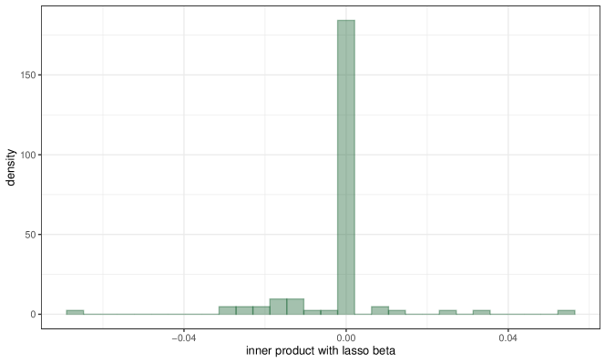
In Section 4 we mentioned the degeneracy when applying a sparse estimate of discriminant direction (Lasso or LDA) directly as the projection direction. We present a simulated distribution of
| (65) |
in Figure E.7, where the intermediate quantities are similarly calculated as in (10). Under the global null, cross-validated logistic Lasso vectors have a positive probability taking exactly zero (i.e. the tallest bar in the histogram is exactly zero rather than a very small number), indicating a non-Gaussian distribution of .
Appendix F Proof of Corollary 4.1
Proof.
To show that is asymptotically normal under the conditions in Corollary 4.1, we essentially need to show the difference between and is of order , where
After recalling and aggregation over the splits, we will conclude that and asymptotically differ by . Formally, for any :
| (66) | ||||
We define a deterministic sequence in step such that: 1) it converges to as and 2)
| (67) |
Such a sequence always exists so long as (we show this formally in Lemma F.1).
The second event in (66) is bounded automatically by definition of .
Lemma F.1.
Given any positive random variable sequence , there exists a deterministic positive sequence such that
-
•
, and
-
•
.
Proof.
Define/Initialize for all , we are going to use an algorithm to update to make it have the desired properties. By definition of , there exists a smallest integer such that
| (71) |
We update to be for all . Similarly, there exists a smallest integer such that
| (72) |
If , we redefine to be . We update to be for all (so right now looks like ). We can repeat the above procedure for all positive integer . Note that for each given , the update of can only happen at most times (due to our “plus-one” step when ), therefore is well-defined for all .
Now we are going to show the constructed having the desired properties. It is direct to check it is a non-increasing, non-negative sequence, therefore it is a convergence sequence. Since can be smaller than any fixed positive number, we know .
Next, we show . For any , we use to denote the largest positive integer such that . By the definition of ,
| (73) |
for all . Specifically, the above property holds when : . By our construction of , . So,
| (74) |
for any . For any , there exists a such that , for all , therefore
| (75) |
∎
Appendix G More Details on Simulated Data
We will use the notation that is a vector of length whose elements are all equal to and is an identity matrix of dimension .
We need to define a preliminary covariance matrix to describe the “normal part” of the generating distribution.
| (76) |
where
| (77) | ||||
We use the following scheme to generate the samples (group 2 samples can be done similarly, replacing by ):
-
1.
Draw a normally distributed sample from . The mean vector varies according to different settings—we will describe them later.
-
2.
Mask with zeros: For each dimension of this preliminary sample, , we generate an independent binary variable such that . If , we change to . Otherwise, we do not modify . The resulting zero-inflated sample is our final observed .
It is possible to formally keep track of the first two moments of and . Specifically, denote , we know:
| (78) |
The covariance matrix can be approximated by a rank-2 matrix. Denote the eigenvalues of it as , we have:
| (79) | ||||
The first two eigenvectors of are still presented in (77).
The means are more straightforward: , .
Now we present the details of each setting: global null, projected null, and alternative.
Under the global null , we set
| (80) |
For the projected null case:
| (81) | ||||
Under the above projected null setting, whereas .
Under the alternative, we chose:
| (82) | ||||
To get more variety of the simulation, we purposely put more signal on the second eigenvector direction (mathematically, ). In this case, is not the optimal direction to project onto and we are curious about the behavior of the proposed estimators.
Appendix H More Details on Real Data Analysis
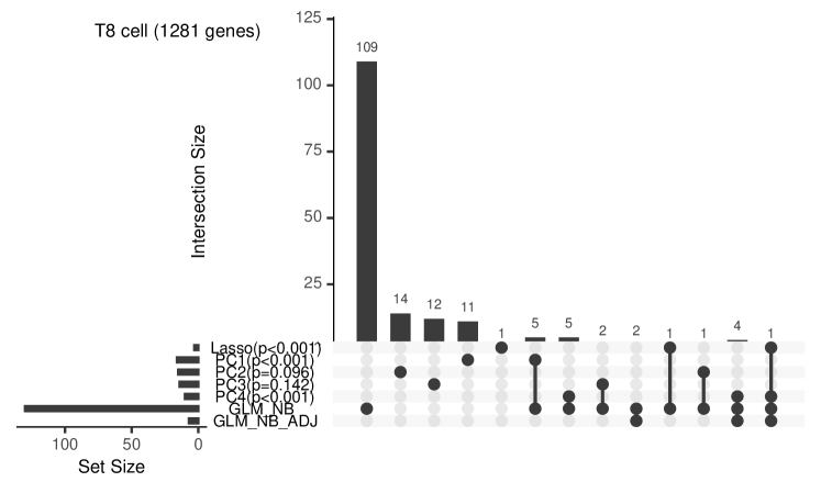
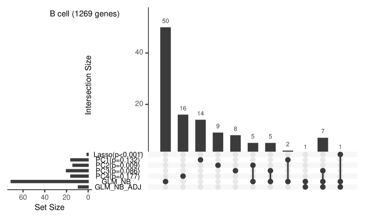
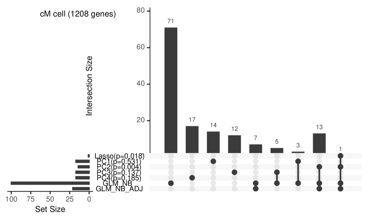
In the main text Section 6, we presented the support gene results for T4 cells. In this section, we also provide the analysis results for the other three types of immune cells in Figure H.9 - H.11.
In Figure H.12, we give a zoomed-in assessment of PC4 support genes (panel A). If one were only interested in protein-encoding genes, the mitochondria genes would have been removed from the analysis, which would give a visually different correlation block (panel B).