Cloud-by-cloud Multiphase Investigation of the Circumgalactic Medium of Low-redshift Galaxies

Sameer,^1,2 Jane C. Charlton,¹ Bart P. Wakker,³ Glenn G. Kacprzak,^4,5 Nikole M. Nielsen,^4,5 Christopher W. Churchill,⁶ Philipp Richter,⁷ Sowgat Muzahid,⁸ Stephanie H. Ho,⁶ Hasti Nateghi,^4,5 Benjamin Rosenwasser,⁹ Anand Narayanan,¹⁰ Rajib Ganguly¹¹
¹Department of Astronomy & Astrophysics, 525 Davey Lab, The Pennsylvania State University, University Park, PA 16802, USA
²Department of Physics & Astronomy, Nieuwland Science Hall, The University of Notre Dame, Notre Dame, IN 46556, USA
³Department of Astronomy, University of Wisconsin-Madison, 475 N. Charter Street, Madison, WI 53706, USA
⁴Centre for Astrophysics and Supercomputing, Swinburne University of Technology, Hawthorn, Victoria 3122, Australia
⁵ ARC Centre of Excellence for All Sky Astrophysics in 3 Dimensions (ASTRO 3D)
⁶Department of Astronomy, New Mexico State University, Las Cruces, NM 88003, USA
⁷ Institut für Physik und Astronomie, Universität Potsdam, Haus 28, Karl-Liebknecht-Str. 24/25, D-14476, Potsdam, Germany
⁸ IUCAA, Post Bag-04, Ganeshkhind, Pune, India - 411007
⁹Department of Physics & Astronomy, The University of Toledo, Toledo, OH 43606, USA
¹⁰Department of Earth and Space Sciences, Indian Institute of Space Science & Technology, Thiruvananthapuram 695547, Kerala, INDIA
¹¹College of Innovation & Technology, University of Michigan-Flint, 196 Murchie Science Building, 303 Kearsley Street, Flint MI 48502, USA
E-mail: sameer@nd.edu

(Accepted XXX. Received YYY; in original form ZZZ)

Abstract

The pervasive presence of warm gas in galaxy halos suggests that the circumgalactic medium (CGM) is multiphase in its ionization structure and complex in its kinematics. Some recent state-of-the-art cosmological galaxy simulations predict an azimuthal dependence of CGM metallicities. We investigate the presence of such a trend by analyzing the distribution of gas properties in the CGM around 47 $z<$ 0.7 galaxies from the Multiphase Galaxy Halos Survey determined using a cloud-by-cloud, multiphase, ionization modelling approach. We identify three distinct populations of absorbers: cool clouds ( $T\sim$ 10^4.1 K) in photoionization equilibrium, warm-hot collisionally ionized clouds ( $T\sim$ 10^4.5-5 K) affected by time-dependent photoionization, and hotter clouds ( $T\sim$ 10^5.4-6 K) with broad O vi and Ly $\alpha$ absorption consistent with collisional ionization. We find that fragmentation can play a role in the origin of cool clouds, that warm-hot clouds are out of equilibrium due to rapid cooling, and that hotter clouds are representative of virialized halo gas in all but the lowest mass galaxies. The metallicities of clouds do not depend on the azimuthal angle or other galaxy properties for any of these populations. At face value, this disagrees with the simplistic model of the CGM with bipolar outflows and cold-mode planar accretion. However, the number of clouds per sightline is significantly larger close to the minor and major axes. This implies that the processes of outflows and accretion are contributing to these CGM cloud populations, but that they are well mixed in these low redshift galaxies.

keywords:

galaxies: groups: general – galaxies: interactions – quasars: absorption lines

^†^†pubyear: 2024

1 Introduction

The circumgalactic medium (CGM) of a galaxy is the tenuous gaseous medium permeating the space beyond the interstellar medium (ISM) and extending out to its virial radius (Kacprzak et al., 2008, 2010; Chen et al., 2010; Steidel et al., 2010; Tumlinson et al., 2011a, 2017; Rudie et al., 2012; Burchett et al., 2013; Nielsen et al., 2013a, b; Werk et al., 2013; Johnson et al., 2015; Lehner et al., 2020). The CGM plays a vital role in galaxy evolution by moderating gas flows between the ISM and the intergalactic medium (IGM). A diverse array of processes such as pristine inflows from the intergalactic medium, galactic-scale outflows, recycled accretion via the galactic fountain mechanism, tidal interactions via satellite galaxy mergers, and effects of cosmic rays and magnetic fields, influence the properties of the CGM. Understanding how these processes manifest in the observed properties of the CGM is a crucial step in understanding galaxy formation and evolution.

The chief ingredients in galaxy formation and evolution models include: 1) accretion of metal-poor inflowing gas from the IGM through filaments onto galaxies (e.g., Oort 1970; Wakker & van Woerden 1997; Wakker et al. 1999; Fumagalli et al. 2011; Stewart et al. 2011, 2013, 2017; Danovich et al. 2012, 2015; Oppenheimer et al. 2012; van de Voort & Schaye 2012; Shen et al. 2013; Kacprzak et al. 2016; Borthakur 2022). 2) recycled accretion from previously ejected metal-rich large-scale galactic outflows (Springel & Hernquist, 2003; Kereš et al., 2005; Dekel et al., 2009; Oppenheimer et al., 2010; Davé et al., 2011a, b, 2012; Stewart et al., 2011; Rubin et al., 2012; Ford et al., 2014; Anglés-Alcázar et al., 2017; Zheng et al., 2017; Hafen et al., 2019; Lochhaas et al., 2020; Pandya et al., 2020, 2021; Fielding & Bryan, 2022). Accretion, in these forms, is necessary to sustain the formation of stars over billions of years (e.g., van den Bergh 1962; Pagel & Patchett 1975; Pagel 1989; Chiappini et al. 1997; Maller & Bullock 2004; Dekel & Birnboim 2006). 3) Outflows from galaxies are needed to regulate the rate of star formation within galaxies by removing gas from the ISM (e.g., Shapiro & Field 1976; Bregman 1980; Kacprzak et al. 2008; Oppenheimer et al. 2010; Faucher-Giguère et al. 2011; Oppenheimer et al. 2012). Outflows carry enriched material out of the galaxy and into the CGM, and are characterized by relatively high metallicities compared with material reaccreting onto the galaxy. On the other hand, pristine accretion is expected to have even lower metallicities.

Recent cosmological magnetohydrodynamical simulations of galaxy formation (e.g., Illustris TNG50, Nelson et al. 2019; Pillepich et al. 2019; Péroux et al. 2020) find that gas with the highest metallicities preferentially aligns with the minor axis, and the highest CGM gas metallicities are associated with high-velocity outflowing gas from the concerted feedback action of supernovae as well as from AGN. The lower metallicities, on the other hand, are associated with accreting/inflowing gas along the major axis. Thus CGM properties, and particularly the distribution of metal-rich gas in the CGM, are anisotropic according to these high-resolution simulations, with metallicity differences of $\sim$ 0.5 dex.

Contrary to these theoretical expectations, previous studies, e.g., Pointon et al. (2019) (hereafter P19), have not found a dependence of metallicity on galaxy azimuthal angle. This was unexpected given that a bimodality is found in distribution of the azimuthal angle of Mg ii absorbers (Bordoloi et al., 2011a, 2014; Bouché et al., 2012; Kacprzak et al., 2012b, 2015a; Rubin et al., 2014; Lan & Mo, 2018; Martin et al., 2019; Dutta et al., 2021; Lundgren et al., 2021). However, consistent with the results on outflow and accretion in hydro-dynamical simulations, Wendt et al. (2021) identify metal enrichment of $\lesssim$ 1 dex for sightlines along the minor axis compared with sightlines along the major axis, using dust depletion as a proxy for metallicity. They argue that metals deplete onto dust grains preferentially along the minor axis, thus needing to account for the dust when estimating metallicities. Their results are based on only 13 galaxy-Mg ii absorber pairs (9 $-$ 81 kpc distance) from the MusE GAs FLOw and Wind (MEGAFLOW) survey at 0.4 $<z<$ 1.4 (Wendt et al., 2021). However, this work is only applicable to damped Ly $\alpha$ absorbers (DLAs) limiting the usefulness of this approach to other lower column density H i-absorbers.

The findings of an association between galaxy azimuthal angle and metal absorption properties are based primarily on observations using Mg ii absorption. However, CGM gas is observed to be multiphase and must be investigated accounting for the contribution of all the gas phases traced by low, intermediate, and high ionization gas, to the H i Lyman series lines in the metallicity determination. Information is lost by assuming an integrated single-valued metallicity per sightline. For simulated absorption profiles, Churchill et al. (2015) and Peeples et al. (2019) found that gas arises in a wide range of structures and physical locations. In addition, there might be little physical overlap between multi-phase gas structures that contribute to the same absorption components (Marra et al., 2022).

Even a single line of sight through the CGM of a galaxy would be expected to have complex multiphase structure with a range of properties. The latest efforts to model observed systems find just that, with metallicities often varying by one or two orders of magnitude along the line of sight through a single absorption system (Lehner et al., 2019; Wotta et al., 2019; Zahedy et al., 2019a; Sameer et al., 2021; Narayanan et al., 2021; Haislmaier et al., 2021; Lehner et al., 2022). Observational investigations of individual absorbers have identified a variety of metallicities within a single absorption system, indicating that CGM characteristics vary along each sight-line (e.g. Churchill et al., 2012; Crighton et al., 2015; Muzahid et al., 2015; Rosenwasser et al., 2018; Zahedy et al., 2019a; Nielsen et al., 2022). Therefore it is important to move beyond observational modelling efforts that typically average together properties (e.g., Pointon et al. 2019) and conduct a large statistical study to determine if the metallicities of any of the multiple structures in the CGM depend on orientation. This will allow us to disentangle the complex nature of the CGM and possibly identify a hidden metallicity/azimuthal bimodality.

Ionization modelling in observational work is often limited to the characterization of the low ionization absorption, which contributes the most to the absorption seen in H i. The properties of the cooler gas phases which typically dominate the H i optical depth are captured by single-phase ionization models (Marra et al., 2021), while the warm-hot phases are often left unaccounted for. Observationally, constraining the properties of high ionization gas traced by O vi has been challenging because the O vi exhibits a significantly broader velocity profile compared with the nearby H i absorbers, and often with misaligned O vi kinematics (e.g., Fox et al. 2013; Savage et al. 2014; Werk et al. 2016). Thus it is often excluded from single-phase ionization modelling. The multiphase nature of the CGM can only be fully understood by analyzing, in combination, the absorption line diagnostics from low, intermediate, and high ions.

In this study, we reanalyze the P19 sample using a cloud-by-cloud, multiphase, Bayesian ionization modelling method. This approach will allow us to delineate the phase structure along the line of sight and ascertain the contribution of multiphase gas to the H i absorption. The P19 sample is unique because all 47 galaxies at redshift $z<0.7$ : 1) have galaxy imaging with HST, which is essential for the determination of azimuthal angles; 2) have UV HST/COS spectra in the MAST archive mostly from PIDs 13398 (P.I. Christopher Churchill) and 11598 (P.I. Jason Tumlinson), with 36/47 absorption systems supplemented with high-resolution optical spectra, covering a range of ionization states including the H i series, O vi, C iv, and Mg ii using optical spectra. This paper is organized as follows: in Section 2 we describe the spectral observations that are analysed in this work; in Section 3.1 we describe the methodology used to determine the physical conditions of an absorber; in Section 4 we present the ionization modelling of all the absorbers in our sample; in Section 5 we present the results from our ionization modelling; in Section 6 we discuss the implications based on the inferred absorption properties seen along these sightlines. We conclude in Section 7. Throughout this work, we assume a $\Lambda$ CDM cosmology with $H_{\_}{0}\,=\,70$ km s^-1 Mpc^-1, $\Omega_{\_}{\rm M}\,=\,0.3$ , and $\Omega_{\_}{\Lambda}\,=\,0.7.$ Metallicities are given in the notation $\log Z/Z_{\sun}$ with solar relative abundances taken from Grevesse et al. (2010). All the distances given are in physical units. All the logarithmic values are presented in base-10.

2 OBSERVATIONS AND DATA

Table 1: Quasar Observations

(1)

(2)

(3)

(4)

(5)

(6)

(7)

(8)

(9)

(10)

(11)

(12)

(13)

J-Name

Proper Name

z_{\_}{\rm qso}

DEC

COS

STIS

FUSE

FUSE

Optical

(J2000)

Gratings

PID(s)

Gratings

PID(s)

Gratings

PID(s)

Spectrograph

PID(s)

a

For the J0456 sightline, we also use the GHRS G200M spectrum from the PID = 5961.
b

Spectra from Churchill & Vogt (2001).

We study the distribution of CGM properties using the “Multiphase Galaxy Halos” Survey, which consists of the HST program with PID 13398 (Kacprzak et al., 2015b, 2019; Muzahid et al., 2015, 2016; Nielsen et al., 2017; Ng et al., 2019; Nateghi et al., 2021) and data from the literature (Yuan et al., 2002; Danforth et al., 2010; Meiring et al., 2011; Churchill et al., 2012; Shull et al., 2012; Tilton et al., 2012; Werk et al., 2013; Fox et al., 2013; Tilton & Shull, 2013; Mathes et al., 2014). HST imaging and UV spectra are available for all 29 quasar fields.

This sample consists of 47 galaxies with spectroscopic redshifts between 0.07 $<z<$ 0.66, which have an impact parameter range of 21 kpc $<D<$ 276 kpc from a background quasar. Two absorption systems in P19, the $z=$ 0.2198 absorber towards the quasar J1139 and the $z=$ 0.2013 absorber towards the quasar J1342, are not considered in our analysis, as for these systems the strongest observed potential H i line (Ly $\beta$ and Ly $\alpha$ , respectively) cannot be disentangled from a complex set of lines from higher-redshift systems, and there are no associated metal lines. Two new systems not presented in P19 are presented in this work. These are the $z=$ 0.1538 and $z=$ 0.3900 absorber towards the quasar J2253. The properties of the galaxies associated with these two systems were determined by and presented in Nateghi et al. (2023). The properties of the remaining galaxies are adopted from P19. For the convenience of the reader, we reproduce Table 2 from P19 and present it in Table LABEL:tab:obsgal. Additionally, we have added the columns of virial radii of the galaxies estimated using the halo masses, impact parameter scaled by the virial radius, absorber velocity scaled by the circular velocity of the galaxy (see § 5.2.4), and information on specific star formation. The propagation of asymmetric uncertainties is carried out using the asymmetric_uncertainty (Gobat, 2022) Python package. The galaxies in this sample are isolated such that they have no neighbors within 100 kpc and have a line-of-sight velocity separation $>500$ km s^-1 from the nearest galaxy P19. This selection minimizes the effect of mergers on the CGM. The halo mass range of the galaxies in the sample is $10.8<\log M_{\_}{h}/M_{\_}{\odot}<12.5$ , which is typical for $L_{\_}{\star}$ galaxies. Galaxy morphologies and other properties for each of the galaxy-absorber pairs in the “Multiphase Galaxy Halos” survey are from Kacprzak et al. 2015b, 2019; Muzahid et al. 2015, 2016; Nielsen et al. 2017; Pointon et al. 2017, 2019; Ng et al. 2019, and from the literature (Chen et al. 2001; Chen & Mulchaey 2009; Prochaska et al. 2011; Werk et al. 2012, 2013; Johnson et al. 2013). We define $\Phi=$ 0^∘ and $\Phi=$ 90^∘ as the projected major and minor axes. The survey reaches an average limiting magnitude of $\approx$ 26 for a S/N of $\approx$ 10, in an average exposure time of $\approx$ 800 s.

2.1 UV Quasar Spectra

The UV spectra in this study were acquired with the COS and STIS instruments onboard the HST telescope, and the LiF and SiC2 channels onboard the $FUSE$ telescope. While P19 have used only the COS G130M and/or G160M when available, and the STIS/E140M for the sightline towards J1704, we have complemented HST/COS observations with $FUSE$ and HST/STIS observations whenever available. The data from these additional gratings often provide better constraints on the inferred absorber properties. The UV $HST$ /COS spectra in this study are downloaded from the Barbara A. Mikulski Archive for Space Telescopes (MAST). We use COS data when both STIS and COS are available, owing to the significantly higher S/N of COS data. We use STIS data when a COS observation does not cover a transition of interest. In Table 1, we list the background quasars and various instruments/gratings they have been observed with.

The COS G130M/G160M spectra have an average resolving power of $R\approx 20,000$ and cover a range of ions including the H i Lyman series, C ii, C iii, C iv, Si ii, Si iii, Si iv, N ii, N iii, N v, and O vi. The HST/COS spectra were reduced following the procedures in Wakker et al. (2015). In essence, spectra are processed with the calcos v3.2.1 pipeline and are aligned using a cross-correlation, and then shifted to ensure that (1) the velocities of the interstellar lines match the 21cm H i profile, and (2) the velocities of the lines in a single absorption system are aligned properly. The exposures are then collectively combined by summing total counts per pixel prior to converting to flux. The $FUSE$ observations were processed with the calfuse pipeline (ver 3.2.3). A zero point offset correction was applied using the methods in Wakker (2006). $FUSE$ spectra have an average resolving power of $R\approx 15,000$ . In some cases, where the absorption of interest is affected by the O i $\lambda$ 1302 geocoronal emission, we use the timefilter module from the costools package to filter unwanted data (SUN_ALT $>$ 0) and rerun the calcos pipeline on the filtered data to generate the airglow emission corrected spectrum for the affected portion of the spectrum. The STIS archival observations are available for some of the sightlines with the E230M and E140M echelle gratings. STIS data were processed using the calstis ver. 3.4.2 pipeline to reduce the raw data into 1-D spectrum. E230M and E140M spectra have an average resolving power of $R\approx$ 30,000 and 45,000, respectively.

Continuum normalization was done by fitting a cubic spline to the spectrum. The statistical uncertainties in the continuum fits were determined by using “flux randomization” Monte Carlo simulations (e.g., Peterson et al. 1998), varying the flux in each pixel of the spectrum by a random Gaussian deviate based on the spectral uncertainty. The pixel-error weighted average and standard deviation of 1000 iterations were adopted as the flux and uncertainty, respectively.

2.2 Optical Quasar Spectra

The UV spectra are complemented with the optical spectra, which cover the low ionization transitions of Mg i, Ca i, Na i, Fe i, Mg ii, Ca ii, Fe ii, Mn ii, and Al ii. Some of these transitions are especially useful in resolving the component structure. Optical spectra from Keck/HIRES or VLT/UVES are available for 34 absorption systems with an average resolving power of $R\simeq 40,000$ . The observation IDs and instruments are listed in Table 1. The HIRES spectra were reduced using the Mauna Kea Echelle Extraction (makee) package ¹¹1https://sites.astro.caltech.edu/~tb/makee/index.html. The UVES spectra were reduced using the European Southern Observatory (ESO) pipeline (Dekker et al., 2000) and the UVES Post-Pipeline Echelle Reduction (UVES POPLER) code (Murphy, 2016; Murphy et al., 2019).

3 Cloud-by-cloud multiphase Bayesian ionization modelling

To extract the properties of CGM absorbers, we employ a novel forward-modelling Bayesian inference suite, Cloud-by-cloud, Multiphase, Bayesian, ionization Modelling method (CMBM; Sameer et al., 2021, 2022), which couples ionization modelling from cloudy with nested sampling Bayesian inference techniques. This modelling approach has been tested using both observations (Sameer et al., 2021, 2022) and large cosmological boxes to cosmological zoom-in simulations of the CGM (Hafen, Sameer et al., 2023), and found to obtain observational estimates accurate to within 0.1 dex of the true source values. This method improves the efficiency of component by component modelling that has been successful in recovering the physical conditions for various individual absorbers (e.g. Churchill & Charlton, 1999; Charlton et al., 2000; Ding et al., 2003a; Charlton et al., 2003; Ding et al., 2003b; Zonak et al., 2004; Ding et al., 2005; Masiero et al., 2005; Lynch & Charlton, 2007; Misawa et al., 2008; Lacki & Charlton, 2010; Jones et al., 2010; Muzahid et al., 2015; Crighton et al., 2015; Richter et al., 2018; Rosenwasser et al., 2018; Zahedy et al., 2019b; Norris et al., 2021). CMBM allows for self-consistently modelling the multicomponent, multiphase absorption profiles seen in multiple ionization states. It uses the observed profile shapes in all the available line transitions, allowing us to better capture the multiphase nature of the absorption systems. This procedure eliminates the need for assuming ionization corrections in the estimation of the metallicities of absorbers as it marginalizes over the unknown amounts of ionization corrections to be applied during parameter inference.

Low-density diffuse gas is seldom found in galaxy halos where there are no substantial stellar or extragalactic sources of ionizing radiation. This photoionizing radiation modulates the ionization states, and thus affects the absorption line signatures from CGM gas. A variety of extragalactic photoionization background radiation (EBR) models exist in the literature. The KS19 (Khaire et al., 2019) EBR model uses the latest QSO emissivities, galaxy star formation rates, estimates of H i distribution in the IGM, dust attenuation in galaxies, and the escape fraction of ionizing photons from galaxies. An investigation of the systematic uncertainties in the inferred parameters due to the choice of the radiation field models is presented in Acharya & Khaire (2021) and Gibson et al. (2022). Acharya & Khaire (2021) find a variation of 4–6.3 and 1.6–3.2 times in the inferred density and metallicity, respectively, depending on whether the gas is high or low density. For $z<1$ , Gibson et al. (2022) find that the absorber metallicities increase on average by $\sim 0.3$ dex as the EUV slope is increased from $\alpha_{\_}{\rm EUVB}=-2.0$ to $-1.4$ . We adopt the KS19 default EUV slope of $\alpha_{\_}{\rm EUVB}=-1.8$ .

3.1 Methodology

We first generate a grid of converged photoionization thermal equilibrium (PIE) cloudy models on a 3–D grid, adopting the KS19 EBR model. The gas conditions of CGM absorbers, which are subject to photoionization by the EBR, are functions of the metallicity, density, and temperature. The axes of the PIE grid are $\log Z/Z_{\sun}$ , $\log n_{\rm H}$ , and $\log N(\mbox{H\,{\sc i}})$ . The $\log N(\mbox{H\,{\sc i}})$ functions as a stopping criterion for a given cloudy model. For a PIE model, cloudy determines an equilibrium temperature, $T$ , such that the absorber is in thermal equilibrium with the background radiation field. The ranges for these parameters are $\log Z/Z_{\_}{\sun}$ $\in$ [ $-3.0,1.5$ ], $\log n_{\_}{\hbox{{\rm H}}}$ $\in$ [ $-6.0,2.0$ ], and $\log N(\mbox{H\,{\sc i}})$ $\in$ [11.0, 21.0], and obtained with a 0.1 dex step-size.

The galaxies in our sample have spectroscopic redshifts between 0.07 < $z$ < 0.66. Therefore, we construct the PIE grids at each $z\in$ [0.05, 0.65], with a 0.05 step size. To create large grids of cloudy calculations, we use the grid command in cloudy and generate grids on a distributed system–Stampede ²²2https://www.tacc.utexas.edu/systems/stampede2 cluster. We adopt the cloudy default solar abundance pattern in model generation. We do not account for depletion due to dust or deviations from solar abundance pattern in our model generation. We report any deviations from the solar abundance pattern.

We start by inspecting the spectrum for low ionization transitions viz. Mg ii, Si ii or C ii that can serve as constraining ions to determine the component structure. We obtain a Voigt Profile (VP) fit to the constraining ion to obtain the redshifts, z ${}_{\_}{i}$ , and total Doppler broadening, $b_{\_}{i}$ , parameters for each, $i$ th, component of an absorption system. The VPs are modelled using an analytic approximation (Tepper-García, 2006) and implemented using the VoigtFit package (Krogager, 2018). With this assumed component structure, we optimise over five parameters in each component, the five parameters being $\log Z/Z_{\sun}$ , $\log n_{\rm H}$ , $\log N(\mbox{H\,{\sc i}})$ , b ${}_{\_}{nt}$ , and $z$ . Here b ${}_{\_}{nt}$ is the broadening due to non-thermal processes, and $z$ is the redshift of the absorption component. We use uniform priors for all five parameters, in the range mentioned above for $\log Z/Z_{\sun}$ , $\log n_{\rm H}$ , and $\log N(\mbox{H\,{\sc i}})$ . For b ${}_{\_}{nt}$ we adopt the range $\in$ [0, $b+3\sigma_{\_}{b}$ ], where $b$ is the value determined from the VP fit, and $\sigma_{\_}{b}$ is the uncertainty on $b$ value, and for $z$ in the range $\in$ [ $z-3\sigma_{\_}{z}$ , $z+3\sigma_{\_}{z}$ ], where z is the absorption centroid for the component.

Typically, an absorption component in an absorption system is composed of one or more “clouds”. Each cloud represents a parcel of gas in a specific spatial location with its own unique properties. These different clouds could potentially contribute to the absorption at a given velocity, albeit potentially being spatially at disparate locations (e.g., Marra et al. 2022). In some cases, asymmetry in the component profile can reveal the presence of two clouds. While in other cases, the need for different ionization parameters to explain the range of transitions observed at a given velocity can reveal the need for two clouds to explain the component. It is generally the case that a model that explains the absorption in low-ionization transitions cannot fully account for the absorption seen in intermediate/high ionization states (e.g., Si iii, C iii, Si iv, C iv, N v, O vi, Ne viii). When it is found that there is absorption unaccounted for by the low-ionization gas phases, we include higher ionization transitions as additional constraining ions. This unaccounted absorption may arise in environments where particle-particle interactions dominate over energy exchange with the radiation field. Earlier works (e.g., Tripp et al. 2001, 2011; Narayanan et al. 2011, 2012) which have undertaken the ionization modelling of high-ionization absorbers have shown that this gas phase is dominated by collisional ionization, primarily based upon the large Doppler broadening parameters of the absorption profiles.

Furthermore, in some instances collisional ionization equilibrium (CIE) cannot sufficiently explain the ratios of observed column densities and/or profile shapes (e.g., Savage et al. 2014). For highly ionized gas at temperatures $\lesssim 5\times 10^{6}$ K, and in the presence of external photoionizing radiation, recombination can slow down in comparison to cooling causing the plasma to remain over-ionized compared with what would be predicted from CIE. Departures from CIE become more prominent for high-metallicity gas. Gnat (2017) (hereafter G17) examined the non-equilibrium evolution of photoionized cooling gas and computed the fractional abundances of different ions as a function of temperature, metallicity, and hydrogen number density. We thus model higher ionization gas, by assuming cooling in the presence of external photoionizing radiation, a more realistic scenario than CIE, using the time-dependent photoionized (TDP) ion fractions from Table 11 of G17. In TDP cooling gas, the abundances of the major coolants may be considered to be either in PIE or affected by time-dependent collisional (TDC) processes, depending on the density. However, the abundance of some specific species may differ by a few factors from the TDC/PIE values, and thus we use the TDP ion fractions. We optimize over five parameters in each cloud modelled as a TDP cloud, the five parameters being $\log Z/Z_{\sun}$ , $\log n_{\rm H}$ , $\log T$ , b ${}_{\_}{nt}$ , and $z$ . We use uniform priors on all parameters in the range - $\log Z/Z_{\_}{\sun}$ $\in$ [ $-3.0,0.3$ ], $\log n_{\hbox{{\rm H}}}/\hbox{cm${}^{-3}$}$ $\in$ [ $-6.0,2.0$ ], and $\log T/K$ $\in$ [4.0, 7.0]. The bounds on these priors are set by the model limits obtained by G17. The priors for b ${}_{\_}{nt}$ and $z$ are determined in a way similar to discussed earlier. We do not adopt TDP models to model low ionization phases (e.g., Mg ii, Si ii, C ii) because the G17 models have a lower bound on temperature of 10⁴ K, and, a posteriori in a number of cases we observe narrow Mg ii absorption suggestive of even lower temperatures.

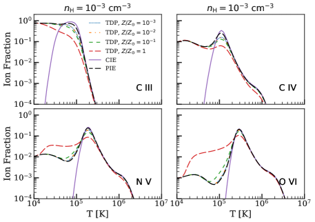
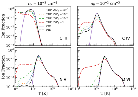
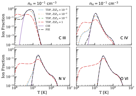
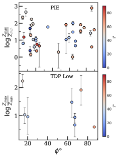
In Fig. 1, we compare the temperature dependence of ionization fractions for gas traced by intermediate and high ionization ions under the various conditions of photoionization equilibrium, collisional ionization equilibrium, and time-dependent photoionization for metallicities $Z/Z_{\_}{\odot}$ = 10^-3, 10^-2, 10^-1, and 1, at the densities of 10^-3 cm^-2, 10^-2 cm^-2, 10^-1 cm^-2. For the intermediate and higher ionization ions of C iii, C iv, N v, and O vi, we observe that the departure between equilibrium models (PIE or CIE) and time-dependent photoionization models is smallest for lower metallicity gas, where the cooling times are longest. The PIE and TDP fractions diverge for metal-enriched gas at temperature, $T\gtrsim$ 10⁴ K. The ionizaton fractions in Fig. 1 show that non-equilibrium ionization can produce significant intermediate and higher ions in a temperature regime often associated with photoionization. While it is possible for the intermediate and higher ionization phases to arise at lower temperatures, by using profile shapes in multiple ionization states in conjunction with the column densities we are able to break the ionization fraction degeneracy. For O vi, at $T\gtrsim$ 4 $\times$ 10⁵ K, the different ionization models are consistent with one another and independent of the density and metallicity, suggesting that CIE is a good approximation for the ionization of O vi gas.

For parameter estimation and model comparison, we use the nested sampling algorithm, PyMultiNest (Buchner, 2014). PyMultiNest is well-suited for tackling multi-dimensional and multimodal posteriors. During the log-likelihood evaluation, the column densities and temperatures from the cloudy grids at the sampled parameter values are calculated on the fly by interpolating over the preconstructed cloudy grid. The interpolant is constructed by triangulating the grid data using the Quick hull algorithm (Barber et al., 1996), and on each triangle linear barycentric interpolation is carried out. We create a “mask” over the regions contaminated by interlopers and over noisy continuum-level regions of the spectrum. The masked regions do not influence the parameter estimation. We perform deblending in cases where there is substantial contribution from Si ii $\lambda$ 989 line to the absorption in N iii $\lambda$ 989 line. For H i-only clouds with no metals detected we adopt 3 $\sigma$ upper limits on the metallicity measurement. To confirm the detection (or lack thereof) of the absorption of interest at the location of H i absorption, we calculate the limiting equivalent width and column density using the pyND³³3https://github.com/jchowk/pyND software.

We compute the Bayes factor to compare models of increasing complexity (more clouds), adopting the model with the highest log-evidence and the least model complexity. In models of increasing complexity, the gain in likelihood does not compensate for the increase in parameters of the model and is found to yield clouds with unconstrained posteriors. We synthesize the expected absorption profiles and compare them to the observed profiles in order to infer the column densities, Doppler parameters, and physical conditions of the absorbing gas. By using the shapes of the absorption profiles and centering of individual components of constraining ions, the CMBM method allows for more robust constraints on inferred model parameters than methods that average together components and perform cloudy modelling of total column densities derived from the data.

4 Absorption profiles and physical conditions

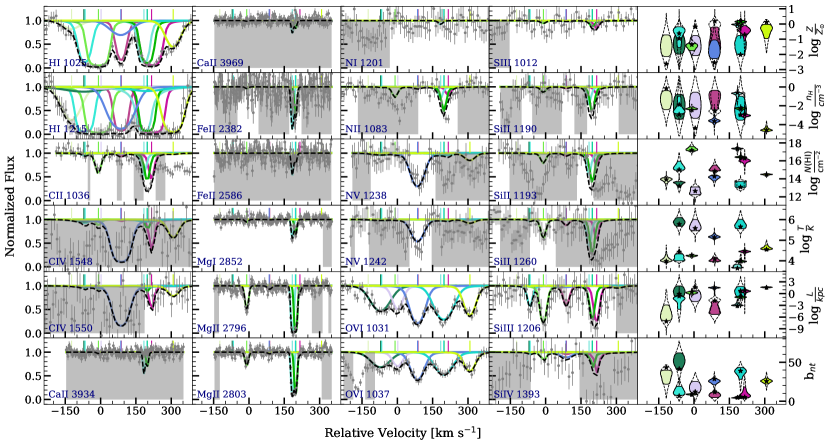
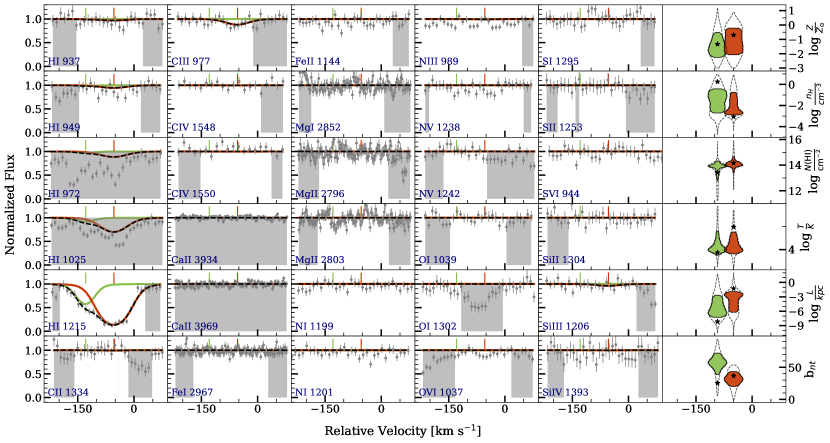
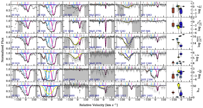
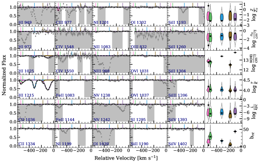
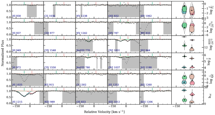
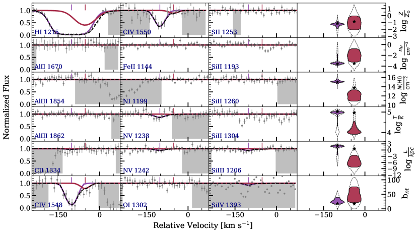
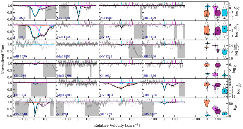
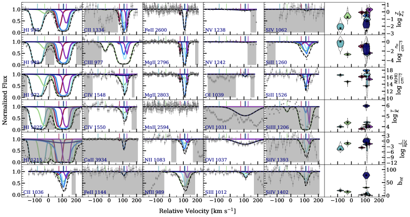
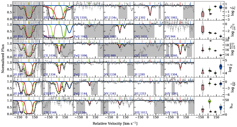
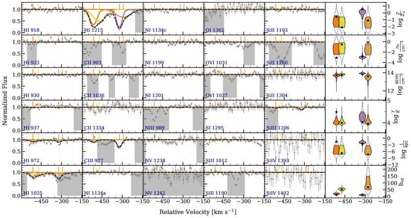
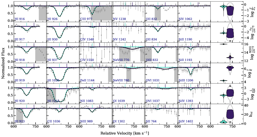
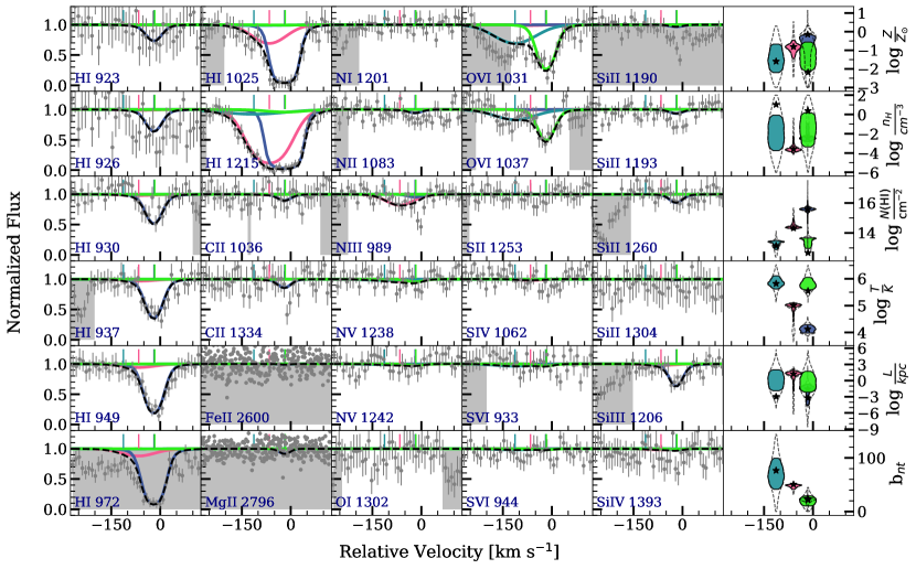
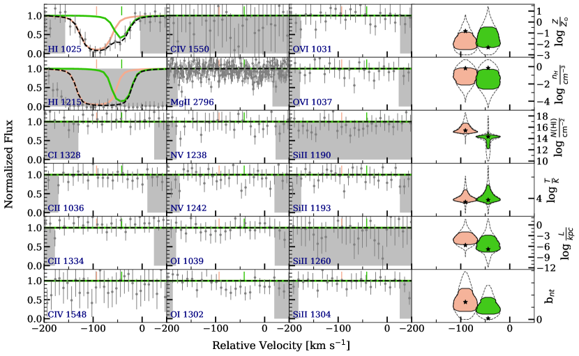
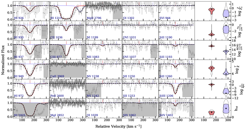
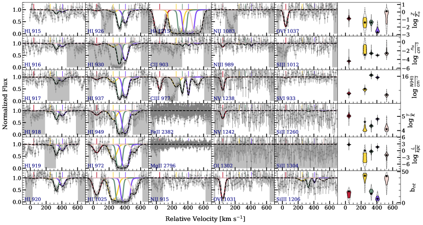
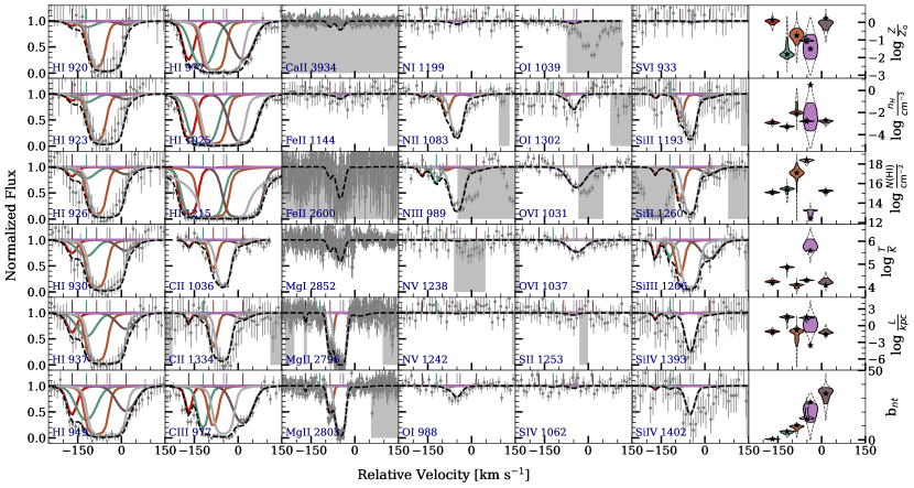
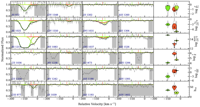
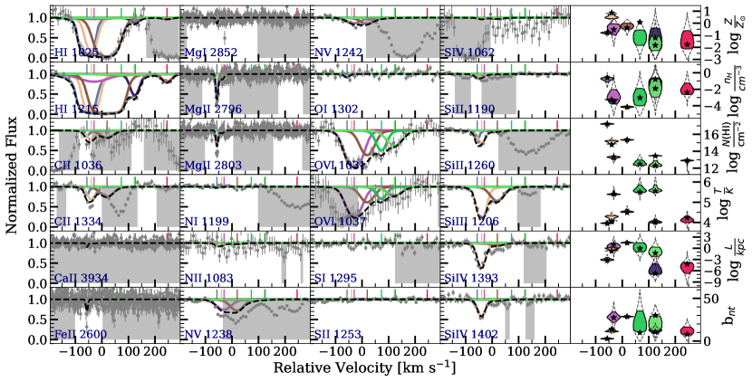
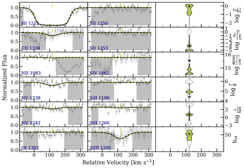
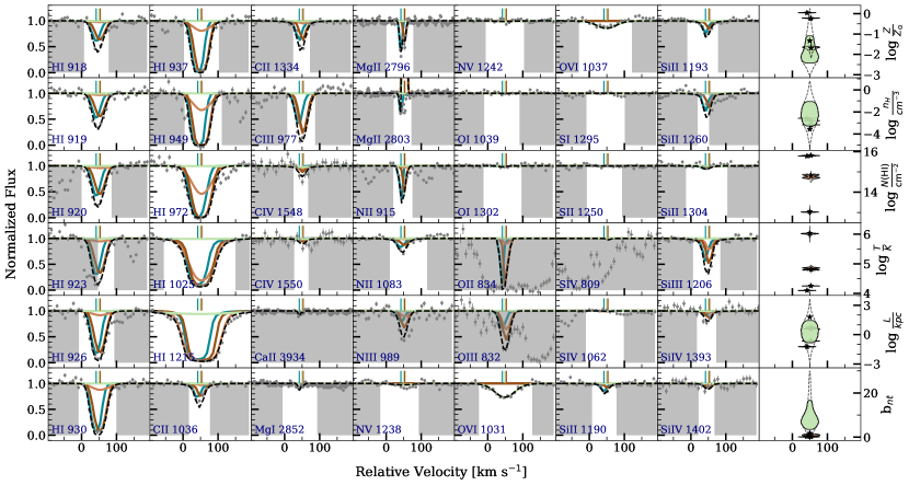
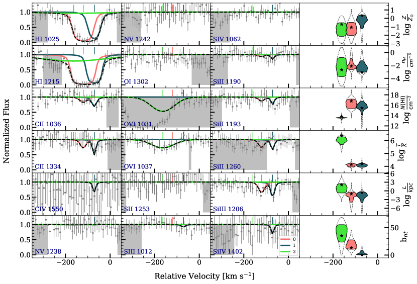
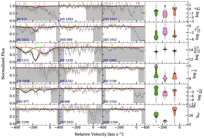
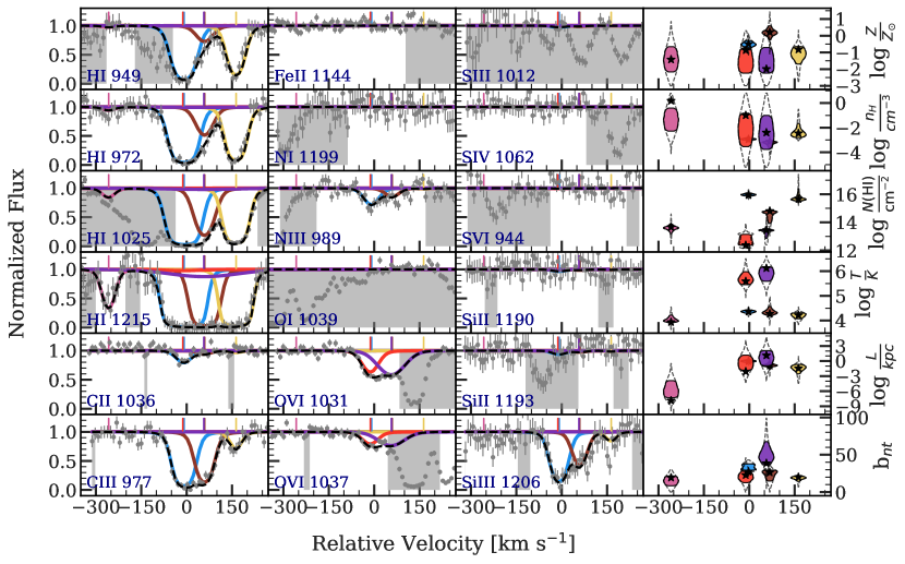
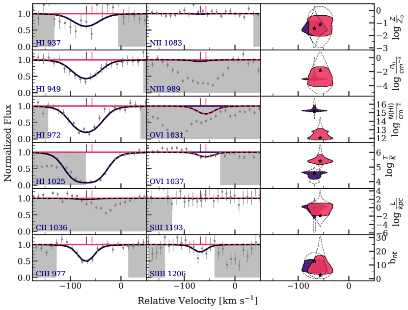
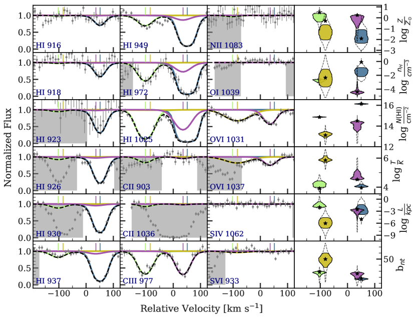
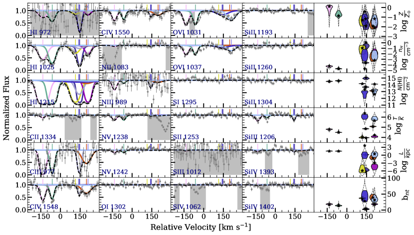
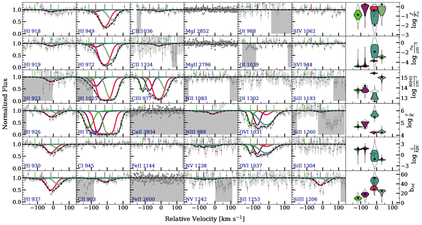
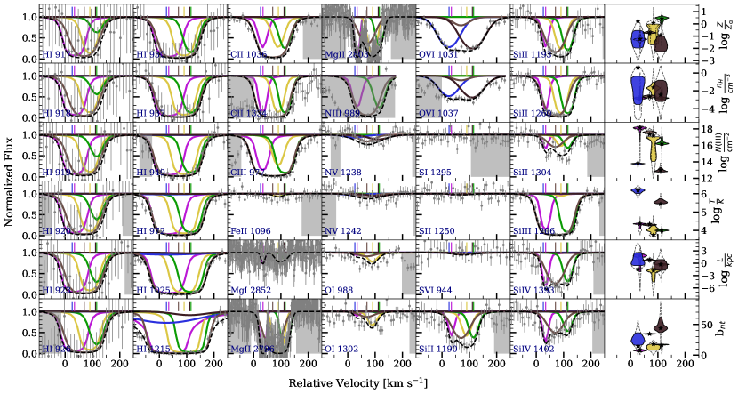
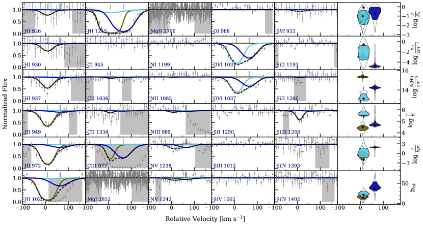
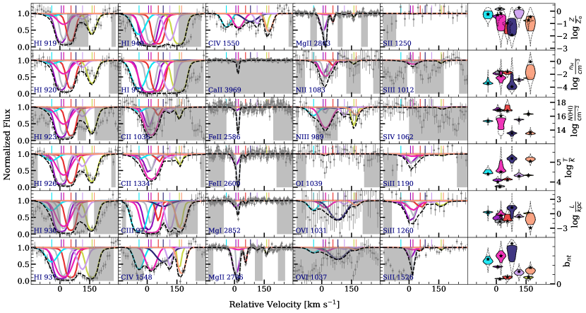
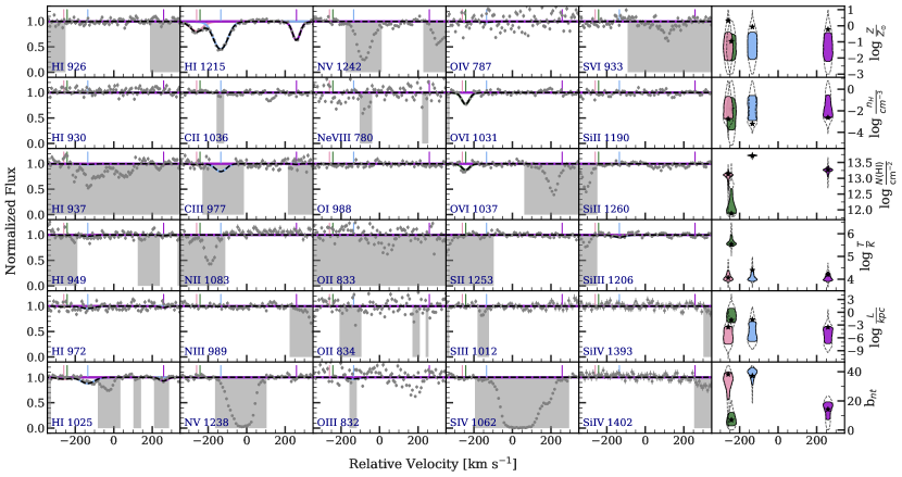
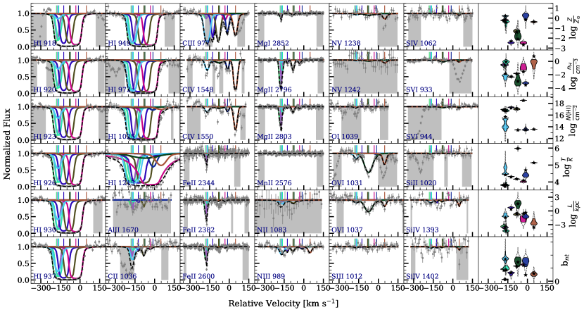
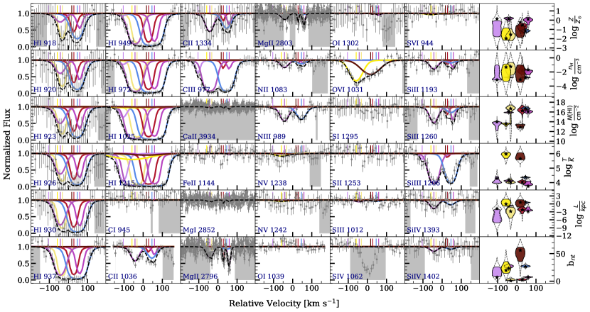
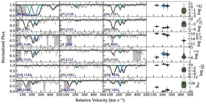
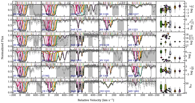
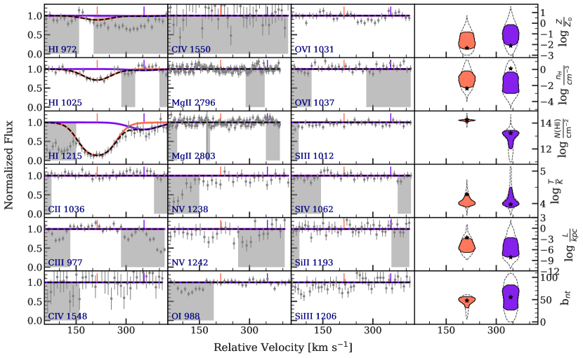
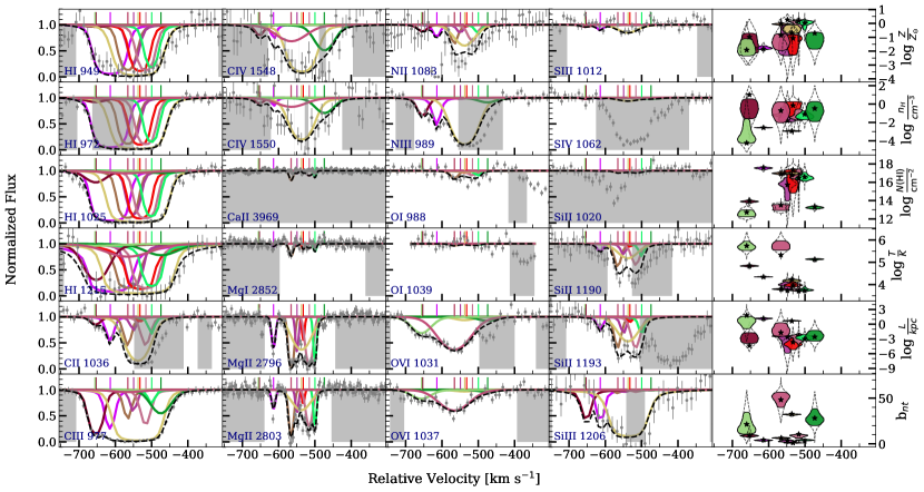
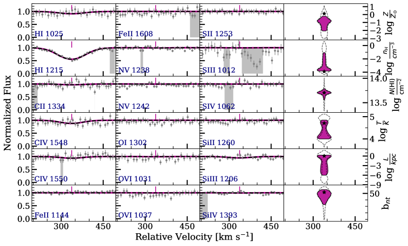
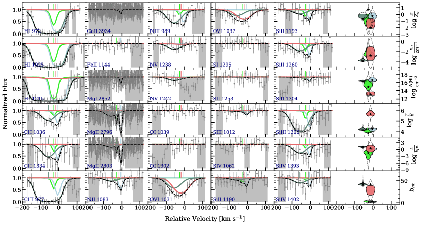
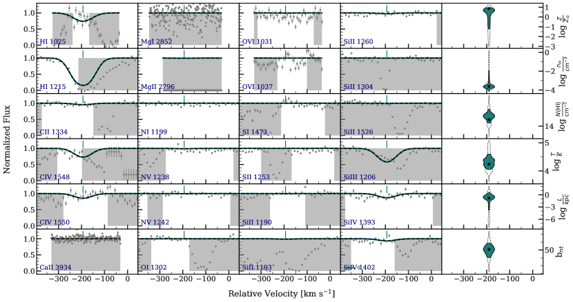
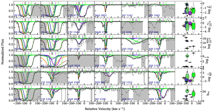
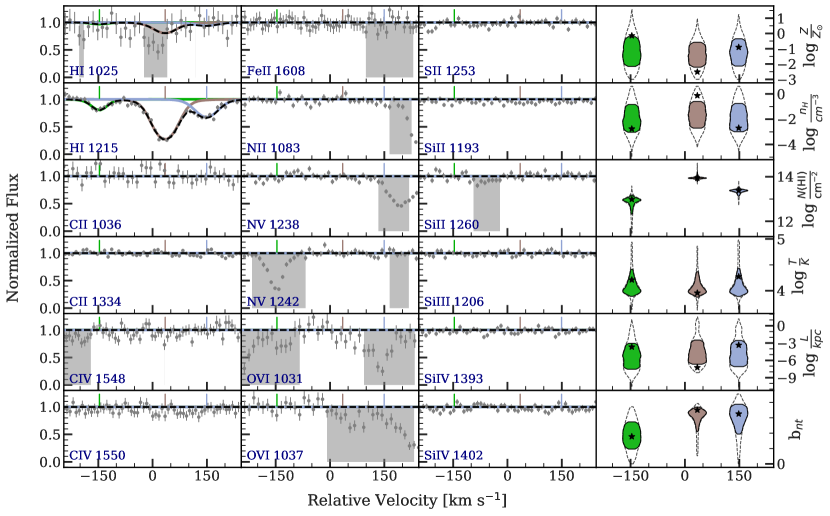
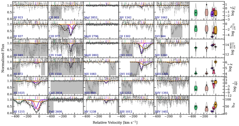
Here, we present the CMBM analysis of the “Multiphase Galaxy Halos” survey. For each absorption system, we present a system plot (e.g., Fig. 21) showing the absorption in various radiative transitions and the Maximum Likelihood Estimate (MLE) ionization models are overlaid on the observed absorption profiles. The observed profiles are presented as a function of velocity relative to the zero-point defined by the redshift of the associated galaxy. The detailed notes on the ionization modelling and system plots for all the systems are presented in appendices B and C, respectively. A summary of the cloud-by-cloud properties of all the individual absorption systems determined by using our CMBM analysis is presented in Table 2.

Based on the models that explain the observed absorption in various phases, we classify clouds into PIE clouds and TDP clouds. Furthermore, for the TDP clouds, we subclassify them into two types–those that show absorption in the high ionization ions of at least the O vi, and possibly N v and/or C iv, but not in the low or intermediate ions, which we refer to as the TDP–High clouds, and those that show absorption in intermediate and high ionization states, and possibly also in low ionization states, which we refer to as the TDP–Low clouds.

In the rightmost panel of every system plot, the inferred marginalised posterior distributions representing the probability distributions of the parameters of interest are presented. The parameters are $\log Z/Z_{\sun}$ , $\log n_{\rm H}$ , $\log N(\mbox{H\,{\sc i}})$ , $\log T$ , $\log L$ , and b ${}_{\_}{nt}$ . The distributions are presented in the form of violin plots to visualise any skewness and multi-modality of the distributions. The region enclosing 99.7% of the distribution is shown as a dotted boundary, and the region enclosing the $16-84$ percentiles is shaded using a colour corresponding to the modelled cloud. The MLE values are indicated as a $\star$ on top of the distributions. In many cases, the MLE provides a good point estimate of the parameters of the distribution. However, it is possible for the MLE to be outside the peak of the distribution. The MLE can be affected by noise in the data which can pull the estimate away from the center of the distribution towards the tail.

For each absorption system, we also discuss the various blends that affect the absorption of interest, and these blended regions are excluded from the modelling. Pixels that are contaminated by absorption from other intervening systems are blanked out and shaded in grey. However, we do not discuss contaminating blends that might appear to be present in a weaker transition but absent in the stronger one, where the line strength is proportional to the product of the oscillator strength and the rest wavelength of the line. We exclude Ca ii from the modeling. Robertson et al. (1988), in the first census of extragalactic Ca ii absorption, found that the Ca ii is severely underabundant compared to both Fe ii and Mg ii, typically smaller by a factor of 100. They argued that the underabundance suggests that Ca ii condenses more readily onto dust grains than Mg ii and Fe ii. Richter et al. (2011) observed a column-density-dependent dust depletion of calcium, finding enhanced dust depletion of Ca ii in high H i column density systems.

Table 2: Cloud-by-cloud properties of the absorption systems

(1)	(2)	(3)	(4)	(5)	(6)	(7)	(8)	(9)	(10)	(11)	(12)	(13)
J-Name	$z_{\_}{\rm gal}$	$V$	$\log Z/Z_{\sun}$	$\log n_{\hbox{{\rm H}}}/\hbox{cm${}^{-3}$}$	$\log N(\rm H)/\hbox{cm${}^{-2}$}$	$\log N(\mbox{H\,{\sc i}})/\hbox{cm${}^{-2}$}$	$\log T/K$	$\log L/kpc$	b_nT	b ${}_{\rm{T}}(\rm{\mbox{H\,{\sc i}}})$	b $(\rm{\mbox{H\,{\sc i}}})$	Ionization Model
		km s^-1							km s^-1	km s^-1	km s^-1

Properties of the different gas phases that contribute to the absorption towards different sightlines. Notes: (1) J-Name of the quasar; (2) Redshift of the galaxy; (3) Velocity of the cloud in the rest frame of the galaxy; (4) cloud metallicity; (5) cloud total hydrogen number density; (6) cloud total hydrogen column density; (7) cloud hydrogen column density; (8) cloud temperature; (9) cloud line of sight thickness; (10) cloud non-thermal Doppler broadening parameter (11) cloud thermal Doppler broadening parameter measured for H i; (12) cloud total Doppler broadening parameter measured for H i; (13) type of ionization model for the cloud; PIE - Photoionized Equilibrium, TDP - Time Dependent Photoionized (see Section 3.1). The marginalised posterior values of model parameters are given as the median along with the upper and lower bounds corresponding to the 16–84 percentiles. The lower and upper limits correspond to $\mu_{\_}{1/2}-2\sigma$ and $\mu_{\_}{1/2}+2\sigma$ , respectively. The rest of the table is presented in appendix B.1.

5 Results

We present the metallicity analysis of the “Multiphase Galaxy Halos” Survey using CMBM analysis of the 47 absorption systems associated with 47 galaxies with well characterized properties. We resolved the absorption in these systems into 240 clouds. These absorbers were found to be explained by one of three kinds of models PIE (157 absorbers in number), TDP–Low (35 absorbers in number), or TDP–High (48 absorbers in number). We plot the various properties to visualize the range and trends, summarize them using the interquartile range (IQR) to capture the dispersion, and the median and the standard deviation of the median from bootstrapped estimates to capture the central tendency of the data. The IQR is calculated as the difference between the 75th and 25th percentiles of the data. Table LABEL:tab:summarystat summarizes the summary statistics of the properties of different cloud types.

In addition to the distribution of metallicities, we also consider the relationship between metallicity and other intrinsic absorber properties including H i column density, total hydrogen column density, temperature, total hydrogen number density, line of sight thickness, and Doppler parameter. We then compare cloud metallicities to galaxy properties including the impact parameter scaled by the galaxy virial-radius, galaxy azimuthal angle, galaxy colour, halo mass, and redshift. We then examine the connection between the azimuthal angle and the CGM metallicities.

5.1 Metallicity and its relationship with absorber intrinsic properties

5.1.1 Metallicity distributions of clouds, $\log Z/Z_{\sun}$

We present the histograms of the metallicities of different cloud types from our sample in Fig. 2. The summary statistics of metallicity distributions are summarized in Table LABEL:tab:summarystat. The histogram for PIE clouds is shown in panel (a). The median of the metallicity distribution of PIE clouds is estimated to be $\log Z/Z_{\sun}$ = $-0.47\pm 0.10$ .⁴⁴4We used the Kaplan-Meier estimator, implemented using the survfit function in R language to determine the median, accounting for the upper limits on some of the metallicity measurements. To account for random variations in the observations, we obtained 1000 bootstrapped estimates of the median to ascertain the uncertainty on the median. The metallicity distribution for PIE clouds is skewed left with a low fraction of very low metallicity clouds. The hatched distribution is the PDF of the upper limits and corresponds to the metallicity limits of H i-only clouds. These clouds have just H i detected with no associated metal absorption, and we adopt 2 $\sigma$ upper limits for their metallicities. The upper limits on PIE clouds are modelled as uniform distributions because of the inferred broad posterior distributions for these clouds. The range of measured metallicities for PIE clouds is in close agreement with the result of P19. However, they obtain a median metallicity of [Si/H] $\approx-1.3$ . P19 infer a metallicity value using only the low and intermediate ionization phases, by measuring total column densities and performing ionization corrections with the help of cloudy. With the CMBM approach, we are able to measure how much of the H i is associated with the various phases contributing to the absorption, and obtain separate metallicities for various clouds and phases. This difference in modelling, and potentially to some extent the choice of EBR, could explain the disagreement between P19 and our result. P19 adopted HM12 (Haardt & Madau, 2012), while we have used KS19 to model the PIE clouds.

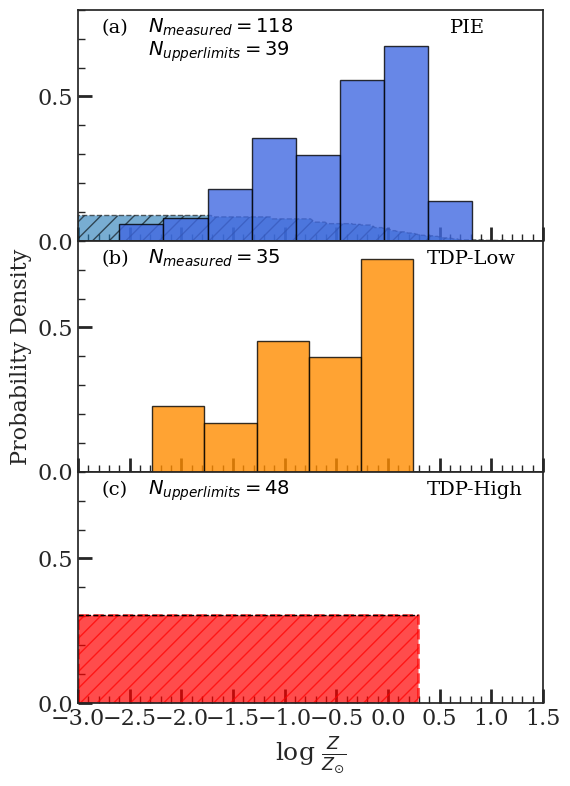
The metallicity distribution of TDP–Low clouds is shown in panel (b) of Fig. 2, and falls in the range [ $-1.1$ , $0.0$ ] with a median metallicity of $\log Z/Z_{\sun}$ = $-0.56\pm 0.21$ . For the TDP–High clouds we display a uniform distribution for their metallicities spanning between [ $-3$ , 0.3] due to the independency on metallicity for these clouds as indicated by their platykurtic posterior distributions.

We compare the metallicity distributions in the context of previous studies that investigated the properties of cool CGM gas. Prochaska et al. (2017) modelled the cool CGM gas of absorbers associated with $z\approx$ 0.2 $L^{\star}$ galaxies and found a median metallicity of [Si/H] = $-0.51$ , with a range of $-1.9$ $\lesssim$ [Si/H] $\lesssim$ 1.0, adopting the HM12 ionizing background. Zahedy et al. (2019a) found a median metallicity of [M/H] = $-0.7\pm 0.2$ , with a 1 $\sigma$ confidence interval of [M/H] = ( $-1.6$ , $-0.1$ ) for absorbers associated with the CGM of luminous red galaxies (LRGs) at redshifts, $0.21\lesssim z\lesssim 0.55$ . The median metallicity of PIE clouds is consistent with the inferred metallicities from these previous works.

5.1.2 Neutral and total hydrogen column density distributions of clouds, $\log N(\mbox{H\,{\sc i}})$ and $\log N(\rm H)$

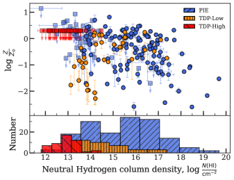
The scatter plots in Figure 3a show the inferred metallicities plotted against the inferred neutral hydrogen column densities for PIE, TDP–Low, and TDP–High clouds. The H i column density of our sample spans several orders of magnitude: $11.8\lesssim$ $\log N(\mbox{H\,{\sc i}})$ $\lesssim 19.7$ . The distributions of neutral hydrogen column densities are presented in the bottom panel. The summary statistics of H i column density distributions for the three cloud types are summarized in Table LABEL:tab:summarystat.

The metallicity of PIE clouds appears to indicate an anti-correlation with the H i column density. We test for the null hypothesis of no correlation between the H i column density and metallicity by computing the Akritas–Theil–Sen (ATS) Kendall correlation coefficient (Akritas et al., 1995) and the associated null-hypothesis probability⁵⁵5This test accounts for the upper limits present on some of the metallicity measurements.. We obtain a $p$ -value of $\approx$ 0.18, suggesting that the null hypothesis cannot be rejected. However, if we just consider those sightlines which are impacting within the virial radius of the galaxy, we find evidence for significant anticorrelation between metallicity and neutral hydrogen column density ( $p$ -value = 0.03). P19 using this same sample of absorbers identified a significant anti-correlation between metallicity and H i column density. However, they found that the correlation vanishes when the HM05 (Haardt & Madau, 2001) EBR is used in ionization modelling instead of HM12 (Haardt & Madau, 2012). Zahedy et al. (2019a) investigated the [M/H] – N(H i) relationship for luminous red galaxies and found no correlation when the HM05 background was used in ionization modelling. Prochaska et al. (2017) also found significant evidence for an anti-correlation between metallicity and H i column density in their analysis of 32 absorption systems from the COS-Halos survey comprising of $L^{\star}$ galaxies using the HM12 EBR. An anticorrelation is also seen for a sample of weak-Mg ii analogs at low- $z$ (Muzahid et al., 2018); they adopted the KS15 EBR (Khaire & Srianand, 2015). The existence of an anticorrelation could be attributed to similarity in the EBR spectrum of KS19 and HM12, both of which have harder spectrum compared with HM05.

Lehner et al. (2019) characterized the metallicities of cool, photoionized gas in the H i-selected Cosmic Origins Spectrograph (COS) circumgalactic medium compendium (CCC) survey (Lehner et al., 2018; Wotta et al., 2019; Lehner et al., 2019), consisting of H i absorbers with column densities ranging between 15 $\leq$ $\log N(\mbox{H\,{\sc i}})$ $\leq$ 19 at $z\lesssim$ 1. Within our PIE sample, we separately tabulate the summary statistics for the metallicities of SLFSs (15 $<$ $\log N(\mbox{H\,{\sc i}})$ $<$ 16.2), pLLSs (16.2 $\leq$ $\log N(\mbox{H\,{\sc i}})$ $<$ 17.2), and LLSs (17.2 $\leq$ $\log N(\mbox{H\,{\sc i}})$ $\leq$ 19) in Table LABEL:tab:summarystat, as these groupings of H i absorbers overlap with the H i-selected absorbers from the CCC survey. We find that the observed range of our metallicity values are consistent with the range of values estimated in the CCC survey. However, our estimated mean values for SLFSs and pLLSs are higher compared to the corresponding values for the CCC survey. The CCC survey obtains mean values of $\log Z/Z_{\sun}$ = $-1.2$ and $-1.3$ for SLFSs and pLLSs, respectively. The metallicities of our LLSs are lower compared with the LLSs in CCC; they obtain a value of $\log Z/Z_{\sun}$ of $-0.6$ . We attribute these differences to the sample selection, our sample is galaxy-selected while the CCC survey is H i-selected. Systematic differences can also stem from the choice of the radiation field. The CCC survey adopted the HM05 radiation field.

The observed relationship between $\log Z/Z_{\sun}$ and neutral hydrogen column density can be directly compared with simulations. Hafen et al. (2017) find that the metallicity distribution of H i absorbers with $\log N(\mbox{H\,{\sc i}})$ $\leq$ 15, the Ly $\alpha$ forest, extends to below $\log Z/Z_{\sun}$ = $-2$ , with many of these absorbers likely tracing IGM gas yet to be enriched by galaxies. We find that a significant percentage ( $57\pm 6$ %) of our absorbers with $\log N(\mbox{H\,{\sc i}})$ $\leq$ 15 are found beyond the virial radius, with no associated metals detected, consistent with results of Hafen et al. (2017). They also find that simulated absorbers with 16.2 $\leq$ $\log N(\mbox{H\,{\sc i}})$ $\leq$ 19 have a metallicity within 1 dex of the mean metallicity of $\log Z/Z_{\sun}$ = $-0.9$ , also consistent with our estimates for this sample.

We also explore the relationship between the metallicity and H i column density of the TDP–Low clouds and find a significant positive correlation ( $p$ -value = 0.007). While we have modelled these clouds assuming time-dependent photoionization, many of these absorbers are found to be overlapping in metallicity with the PIE clouds. We do not interpret this positive correlation as it is quite possible that some of these clouds could be in PIE, depending on their density, complicating the interpretation of the correlation. We do not investigate the trend between the metallicity and neutral hydrogen column density of TDP–High clouds, as their metallicities are unconstrained.

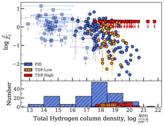
In Fig. 3b, the metallicity is plotted as a function of the total hydrogen column density for different absorber types. The total hydrogen column density of our sample spans several orders of magnitude: $12.9\lesssim$ $\log N(\rm H)$ $\lesssim 22.0$ . The distribution of total hydrogen column densities for PIE clouds seems to show a bimodality, with a smaller peak at $\log N(\rm H)$ $\approx$ 14.6, and a more prominent peak at $\approx$ 18.0. However, Hartigan’s Dip test suggests that the null hypothesis of unimodality cannot be rejected ( $p-$ value = 0.09). We determine that the $\log N(\rm H)$ of H i-only PIE clouds ranges from 12.9 to 17.9, with an IQR of [14.2, 15.0].

The $\log N(\rm H)$ distribution of TDP–Low clouds is quite flat and spans a narrow range of values. The predicted range and median for $\log N(\rm H)$ of TDP–High clouds are consistent with the properties of low redshift, $z<0.5$ , warm O vi absorbers (5.4 $\lesssim$ $\log T$ $\lesssim$ 6.2) from Savage et al. (2014) who obtained a range of 18.4 $<$ $\log N(\rm H)$ $<$ 20.4, and median of $\log N(\rm H)$ = 19.35.

5.1.3 Temperature, $\log T$

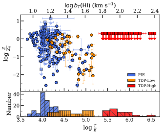
In Figure 4a, we show metallicity as a function of temperature, $\log T$ , plotted on the bottom x-axis. The summary statistics of the temperature distribution for the different cloud types is given in Table LABEL:tab:summarystat. We find that the temperature ranges for these three cloud types agree with the multiphase CGM manifested in hydrodynamic simulations, which exhibit a mixture of cool, warm-hot, and hot phases. The temperature distribution of PIE clouds appears to be right-skewed with a majority of the absorbers concentrated around the median of $T\sim$ 10⁴ K, and a tail extending to $T\sim$ 10⁵ K. The temperature distribution of TDP–Low and TDP–High clouds appears to be flat between $T\sim$ 10^4.2-5.2 K) and ( $T\sim$ 10^5.4-6.0 K), respectively. The temperatures of some of the TDP–High clouds are consistent with Coronal Broad Lyman- $\alpha$ (CBLA) absorbers–the collisionally ionized, million-degree gas hypothesized to be pervading the extended, hot gaseous halos of low-redshift galaxies (e.g., Narayanan et al. 2010; Savage et al. 2010, 2011a, 2011b; Richter 2020).

We perform an ATS test between the $\log Z/Z_{\sun}$ and $\log T$ measurements of the PIE clouds and TDP–Low clouds. For PIE clouds, we obtain a $p$ -value of 0.01, indicating evidence for anti-correlation between these parameters. We also see evidence for anti-correlation between the metallicity and temperature of the TDP–Low clouds ( $p$ -value = 0.005). Higher metallicity allows the gas to cool efficiently, leading to a lower temperature–causing the anticorrelation.

5.1.4 Doppler parameters

The Doppler parameter, $b$ , quantifies the line broadening mechanism, which is influenced by thermal and/or turbulent processes. The thermal motions of the particles result in Doppler broadening of the observed profiles. The thermal Doppler broadening and temperature are related by $b_{\_}{\rm T}=\sqrt{2kT/m}$ km s^-1. In Fig. 4a, we show the metallicity as a function of the thermal Doppler broadening parameter, b ${}_{\rm{T}}(\rm{\mbox{H\,{\sc i}}})$ , plotted on the top-axis in log values.

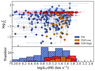
In Fig. 4b, we show the metallicity as a function of the non-thermal Doppler broadening parameter, b_nT, plotted in log values. The non-thermal Doppler broadening parameter in absorbing structures is potentially mediated by post-shock turbulence from outflows and/or accretion (e.g., Cen & Ostriker 2006; Draganova 2015). Magnetohydrodynamic turbulence produced by collisionless shocks could result in a significant non-thermal contribution to the observed line profiles, as observed in TNG100 simulations (Nelson et al., 2018). The non-thermal Doppler broadening distribution of PIE clouds is relatively flat with a lack of pronounced mode, however, there are some clouds with smaller values, suggesting that some of these clouds are predominantly thermally broadened. The non-thermal Doppler broadening distribution of TDP clouds is also flat, but the TDP clouds always show some amount of contribution from non-thermal broadening to their line profiles.

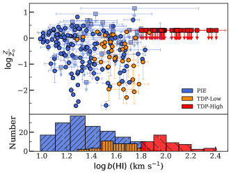
In Figure 5a, we show the metallicity as a function of the total Doppler broadening parameter, b $(\rm{\mbox{H\,{\sc i}}})$ , and the b $(\rm{\mbox{H\,{\sc i}}})$ distribution for different cloud types. The distribution of b $(\rm{\mbox{H\,{\sc i}}})$ for PIE clouds appears broad and ranges between 10–90 km s^-1 with a median of 21.3 $\pm$ 1.2. The COS CGM Compendium (CCC) survey (Lehner et al., 2018) comprising of H i-selected absorbers found a median Doppler broadening parameter of b $(\rm{\mbox{H\,{\sc i}}})$ $\approx$ 28 km s^-1 for gas consistent with being primarily photoionized. The distribution of b $(\rm{\mbox{H\,{\sc i}}})$ for TDP–Low clouds overlaps with that of the right tail of PIE clouds. Richter (2020) who systematically studied the extended, hot gaseous halos of low-redshift with CBLAs, inferred Doppler parameters ranging from 70 – 200 km s^-1. The total Doppler broadening parameter, b $(\rm{\mbox{H\,{\sc i}}})$ , for TDP–High clouds in our sample is consistent with the range determined for CBLAs.

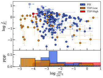
5.1.5 Total hydrogen density, $\log n_{\rm H}$

In our model clouds the total hydrogen density, $\log n_{\rm H}$ , allows the ionization parameter to be well-defined for the adopted EBR spectrum at the redshift of the absorber. In Fig. 5b, we show the metallicity as a function of total hydrogen number density and the histogram of $\log n_{\rm H}$ . The summary statistics of the hydrogen density distribution for the different cloud types is given in Table LABEL:tab:summarystat. The hydrogen density distribution of PIE clouds is right-skewed, with a pronounced peak at the median value of $\log n_{\rm H}$ $\approx-2.5$ . The TDP–Low clouds show a range of hydrogen densities, but there is a higher frequency of these clouds with low densities. For the TDP–High clouds, the posterior distribution of $\log n_{\rm H}$ of the modelled clouds is unconstrained. For gas at $\log T$ $\gtrsim$ 5.4, the ionization of the gas is most likely dominated by collisional ionization since heating by photoionizing radiation is unlikely to produce such high temperatures. For such gas, the radiative cooling efficiencies are functions of the temperature only and independent of density, thus resulting in large model uncertainties, provided the density is high enough ( $\gtrsim$ 10^-4 cm^-3) for particle interactions to become more important than photoionization (Gnat, 2017). Thus, for the TDP–High clouds we adopt a lower limit on their $\log n_{\rm H}$ and their $\log n_{\rm H}$ distribution is presented as a uniform distribution in [ $-4.0,2.0$ ].

5.1.6 Line of sight thickness, $\log L$

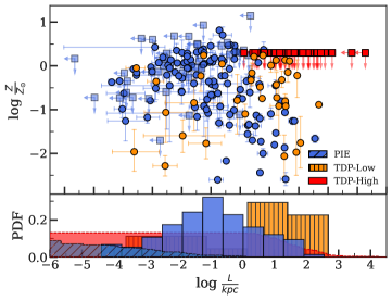
Our models assume that the cloud geometry is plane-parallel, and the ionization structure of the model cloud is determined using the boundary condition set by the neutral hydrogen column density. Using the predicted total hydrogen column density corresponding to the boundary condition, the thickness can be determined using the relation $L=\frac{N_{\_}{\rm H}}{n_{\_}{\rm H}}$ , where N ${}_{\_}{\rm H}$ and n ${}_{\_}{\rm H}$ are the total hydrogen column density and total hydrogen number density, respectively. The summary statistics of the size distribution for the different cloud types is given in Table LABEL:tab:summarystat. In Fig. 6, we show the metallicity as a function of cloud size for the three cloud types. The $\log L$ distribution of PIE clouds appears to be platykurtic, with a median value of $\log L/kpc$ = $-1.4\pm 0.2$ . The TDP–Low clouds show a range of sizes, but there is a higher frequency of these clouds with large sizes. For the TDP–High clouds, because of the dependence of $\log L$ on $\log n_{\rm H}$ , we obtain upper limits on the inferred $\log L$ values. We determine upper limits based on the lower limit of $\log n_{\rm H}$ $\geq-4$ and the model predicted $\log N(\rm H)$ .

5.2 Metallicity and its relationship with galaxy properties

We next examine the trends of metallicity with a set of galaxy properties.

5.2.1 M ${}_{\_}{\rm halo}$

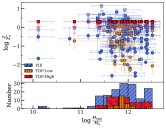
In Figure 7a, we plot the metallicity, $\log Z/Z_{\sun}$ , as a function of the galaxy halo mass, M ${}_{\_}{\rm halo}$ . All the types of clouds are seen for all halo masses. We examine the relationship between metallicity and halo mass for any underlying trends. We do not find evidence to reject the null hypothesis of no correlation between metallicity and halo mass for PIE, TDP–Low, and TDP–High clouds ( $p$ -values $\approx$ 0.75, 0.92, and 0.82, respectively). We also do not find evidence for significant differences in the halo mass distributions of the three groupings.

5.2.2 Galaxy Redshift

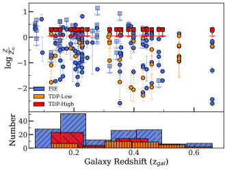
Galaxies and quasars contribute most of the photoionizing radiation at all redshifts and their contribution is known to evolve with redshift (e.g., Gibson et al. 2022). The galaxies in our sample span the redshift range of 0.07 $<z<$ 0.66. We investigate any trends due to the evolution of EBR on how various absorber types would be manifest in our sample. In Figure 7b, we plot the metallicity as a function of galaxy redshift, z ${}_{\_}{\rm gal}$ . We do not see an indication of trend between the metallicity and galaxy redshift for PIE and TDP–Low clouds. These cloud types are found at all redshifts. We do not expect and see the effect of EBR on the properties of TDP–High clouds as these are dominated by collisional ionization.

5.2.3 Impact Parameter

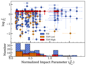
In Figure 8a, we plot the metallicity, $\log Z/Z_{\sun}$ , as a function of the normalized impact parameter, D/ $R_{\rm vir}$ . The PIE clouds and TDP–clouds are found up to 1.7 $R_{\rm vir}$ . We determine that within $R_{\rm vir}$ , $84\pm 3$ % of the clouds show detected metals at the 2 $\sigma$ level, but beyond $R_{\rm vir}$ only $36_{\_}{-8}^{+9}$ % of the clouds show detected metals at the 2 $\sigma$ level. This is indicative of the fact that most of the metals are retained within the $R_{\rm vir}$ of galaxies. We investigate the existence of any trends between these two parameters and find that none of the groupings show evidence for a correlation.

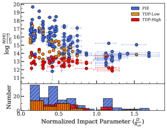
In Figure 8b, we investigate the relationship between neutral hydrogen column density and normalized impact parameter. Previous studies (e.g., Lanzetta et al. 1995; Tripp et al. 1998; Chen et al. 2001; Wakker & Savage 2009; Rao et al. 2011; Werk et al. 2014; Borthakur et al. 2015; Curran et al. 2016; Prochaska et al. 2017; Kulkarni et al. 2022) found that the H i column density declines with increasing impact parameter for CGM absorbers. We also observe a similar trend, consistent with these previous works. The dispersion in neutral hydrogen column densities for PIE and TDP–Low clouds decreases with the normalized impact parameter, while the TDP–High clouds show a similar level of dispersion. We test for correlation for each of the three groupings using the ATS test. For the PIE clouds, mainly tracing the cool CGM gas, we see significant anti-correlation ( $p$ -value $\approx$ 10^-5) between $\log N(\mbox{H\,{\sc i}})$ and D/ $R_{\rm vir}$ . TDP–Low clouds also show significant anti-correlation ( $p$ -value $\approx$ 0.03), while the TDP–High clouds do not show evidence for anti-correlation ( $p$ -value $\approx$ 0.73).

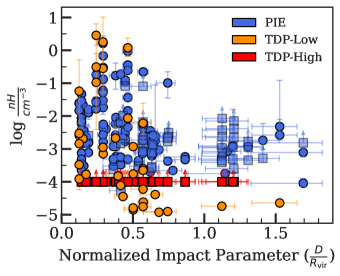
Werk et al. (2014) found an indication of declining hydrogen density as a function of impact parameter scaled to the galaxy virial radius for cool, photoionized CGM gas using the COS-Halos (Tumlinson et al., 2011a) gas column density measurements. In Fig. 9, we plot the hydrogen number density as a function of the normalized impact parameter. For PIE clouds, we observe that within $R_{\rm vir}$ , a large range of hydrogen densities are seen spanning between $\log n_{\hbox{{\rm H}}}/\hbox{cm${}^{-3}$}$ = $-3.7$ to 0.2. However, for impact parameters $>$ $R_{\rm vir}$ we find a narrower range of densities spanning between $\log n_{\hbox{{\rm H}}}/\hbox{cm${}^{-3}$}$ = $-4.0$ to $-2.3$ .

We perform an ATS test to investigate the null hypothesis of no correlation between the hydrogen density and normalized impact parameter. We find significant evidence of a negative correlation ( $p$ -value = 0.01) between these parameters for PIE clouds, excluding the lower limits on hydrogen density. We also find significant evidence for a negative correlation between these parameters for TDP–Low clouds ( $p$ -value = 0.003).

5.2.4 Absorber velocities

Cosmological hydrodynamical simulations (e.g., TNG50; Péroux et al. 2020) predict that the highest metallicities in the CGM are associated with high-velocity outflowing gas expelled from the ISM. On the other hand, gas with lower metallicities is associated with lower velocity accreting or inflowing processes. Simulations (e.g., Ford et al. 2014) also predict that cool photoionized gas traces recycled accretion, warm-hot gas traces both recycled accretion and ancient outflows depending on impact parameter, while hotter gas probes ancient outflows.

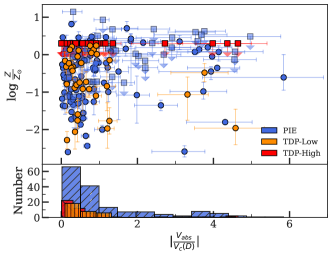
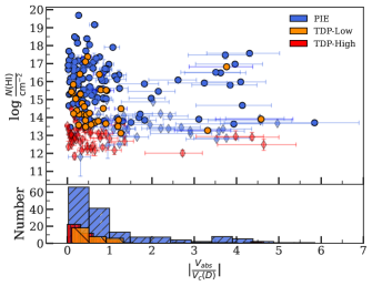
In Figure 10a, we plot the metallicity, $\log Z/Z_{\sun}$ , as a function of absorber velocity scaled by the galaxy circular velocity measured at the impact parameter, | $V_{\rm abs}$ / $V_{\rm c}$ (D)| for different cloud types. Galaxy circular velocities are calculated at the impact parameter of absorption using equation (5) of Navarro et al. (1996) and equation (B2) of Churchill et al. (2013). The velocity zero point is the host galaxy systemic velocity. Accretion is expected to roughly match the rotation velocity of the host galaxy at a maximum, whereas outflows can sometimes exceed the escape velocity of galaxies, especially for lower mass galaxies. But also more massive galaxies can host absorption with higher velocities. Our sample of galaxies spans a range of halo masses; thus, we scale the absorber velocities shifted with respect to the galaxy by the circular velocity at the measured impact parameter of the host galaxy, V ${}_{\_}{c}$ (D) to account for the galaxy halo mass (see e.g., Ng et al., 2019). We tabulate the V ${}_{\_}{c}$ (D) values in Table LABEL:tab:obsgal.

We observe that clouds with high | $V_{\rm abs}$ / $V_{\rm c}$ (D)| show both low and high metallicities; similarly clouds with low | $V_{\rm abs}$ / $V_{\rm c}$ (D)| also exhibit a range of metallicities. We determine that the metal detection fraction for clouds with absolute absorber velocities $\leq$ V ${}_{\_}{c}$ (D) is $85_{\_}{-4}^{+3}$ %, while for clouds with absorber velocities $>$ V ${}_{\_}{c}$ (D) it is only $54\pm 7$ %. This observation likely indicates that material beyond V ${}_{\_}{c}$ (D) is not closely associated with the host galaxy and is likely tracing IGM material. We further investigate if there is an underlying trend by plotting the $\log N(\mbox{H\,{\sc i}})$ as a function of | $V_{\rm abs}$ / $V_{\rm c}$ (D)| in Figure 10b, we see that the data points with upper limits on metallicity are the ones that have low $\log N(\mbox{H\,{\sc i}})$ values, $\lesssim 14.5$ , indicated by lightly shaded diamond markers. At these low $\log N(\mbox{H\,{\sc i}})$ values the expected metal columns are quite low, which are difficult to measure at the resolution of COS and S/N of the observed data. These high-velocity clouds can be reasonably attributed to the fact that the material likely at the periphery of galaxies or in the IGM is unlikely to exhibit a direct connection with the kinematics of the galaxy.

5.2.5 Azimuthal Angle

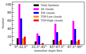
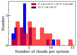
In Fig. 11a, we show the azimuthal angle, $\phi$ , distributions for the number of clouds. We find that there are more PIE clouds along the major axis compared with other angles, with additional enhancement along the minor axis. We create four equal-width azimuthal angle bins: 0^∘–22.5^∘, 22.5^∘–45^∘, 45^∘–67.5^∘, and 67.5^∘–90^∘. Our choice of binning is to ensure that there are a sufficient number of data points in each bin, and the number of systems is nearly evenly distributed in these bins. The total number of absorption systems is 16, 8, 12, and 11 in each of these azimuthal angle bins. The total number of clouds is 101, 28, 52, and 59 clouds in these four bins. We compare the number of clouds per absorption system along the major and minor axis ( $0^{\circ}\leq\Phi\leq 22.5^{\circ}$ $\cup$ $67.5^{\circ}\leq\Phi\leq 90^{\circ}$ ) with the number of clouds per absorption system along the interjacent angles ( $22.5^{\circ}<\Phi<67.5^{\circ}$ ), and show their distributions in Fig. 11b. We see that along the major and minor axes, there is a relatively higher frequency of observing more than $\sim$ 5 clouds per absorption system, compared with the interjacent angles. We compare their distributions using a 2-sample Anderson-Darling test (Scholz & Stephens, 1987) to test the null hypothesis that the distribution of the number of clouds per system along the minor and major axis is different from the distribution of the number of clouds per system along the interjacent angles. This test is particularly suitable for sample sizes of less than 25 observations each. We find statistically significant evidence to reject the null hypothesis ( $p$ -value = 0.03). Berg et al. (2023), in their bimodal absorption system imaging campaign (BASIC) survey, aimed at characterizing the galaxy environments of pLLSs and LLSs at $z\lesssim 1$ , and found that metal-enriched absorbers ( $\rm[X/H]$ $>$ $-1.4$ ) are preferentially found along the major and minor axes, consistent with our observations. We note that a significant percentage, $89_{\_}{-5}^{+4}$ %, of our galaxy-selected pLLSs and LLSs absorbers have metallicities, $\log Z/Z_{\sun}$ $>$ $-1.4$ .

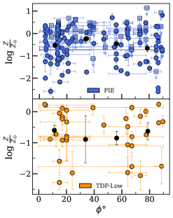
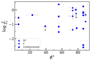
We next examine the spatial distribution of CGM metallicities in Fig. 12a with the bootstrapped mean metallicities in the various azimuthal angle bins overplotted in black. We observe a wide range of metallicities for all azimuthal angles, and observe a similar dispersion in metallicity for all the cloud types for all angles. We find that the mean metallicities are consistent with one another within their uncertainties (standard error on the mean) for each of the cloud types. The bootstrapped metallicity mean and its uncertainty are tabulated in Table LABEL:tab:meanmetallicity_azi. We also perform a log-rank test, accounting for the non-detections, to test the null hypothesis of no difference in metallicities between any two chosen azimuthal angle bins for the three different types of clouds. The inferred $p-$ values from these tests suggest that the null hypothesis of no difference in the metallicity distribution of gas along the minor axis, major axis, and interjacent angles cannot be rejected for all three cloud types.

Veilleux et al. (2005) suggested that outflows should have large cloud-cloud variations in metallicity. Such signals are also observed in very strong Mg ii absorbers (Bond et al., 2001) and at lower column densities (e.g., Rauch et al., 2002; Zonak et al., 2004). In Fig. 12b, we examine this by plotting the metallicity variation, the difference between maximum and minimum metallicities in a given absorption system along a given sightline, with points coloured by their inclination angle. We only plot points corresponding to an absorption system with more than one cloud. We do not observe significant differences in the metallicity variation along the minor or major axis. In the case of TDP–Low clouds, the number of clouds is too low to observe a trend. It is possible that the dependency on other galaxy or gas properties is the cause of scatter in the metallicity distribution as a function of the azimuthal angle. We investigate any such dependency while taking into account the H i-column density, inclination angle, impact parameter scaled by virial radius, $B-K$ galaxy colour, absorber velocity scaled by the galaxy circular velocity, and the halo mass of the galaxy.

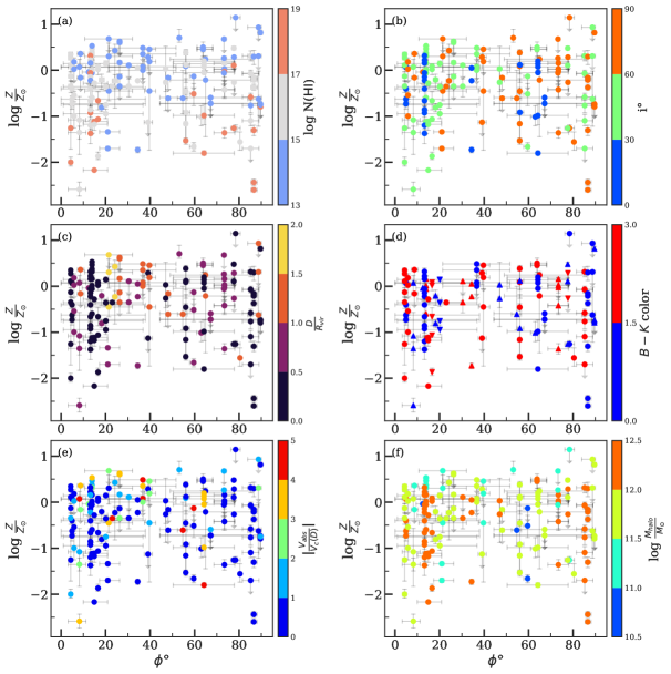
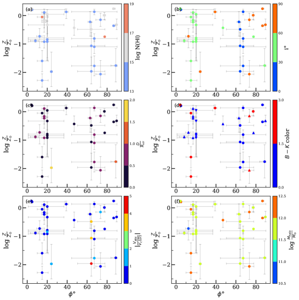
In Figs. 13 and 14, we present the relationship between metallicity and azimuthal angle for PIE clouds and TDP–Low clouds where the data points are coloured by different galaxy properties. In Figure 13a, the data points are coloured by neutral hydrogen column density. We observe that the lowest neutral hydrogen column densities are often upper limits on metallicity, and these low hydrogen column densities are seen at all azimuthal angles. There is also no discernible trend in the association between metallicity and azimuthal angle among the absorbers chosen by H i column density. A metallicity bimodality is expected to be strongest for pLLS due to inflows and outflows (Wotta et al., 2019). We compare the metallicities of pLLSs for the minor and major axis groupings, however, we do not find evidence of a significant difference in their metallicity distributions. This finding suggests that a generalization that metal-poor accretion occurs along the major axis and metal-enriched outflows along the minor axis is too simplistic. Instead, this indicates that the CGM is evenly mixed across the entire range of azimuthal angle and for all H i column densities. We also do not see any evidence of a trend for TDP–Low as well (Fig. 14a).

Furthermore, we take into account how the inclination angle affects the correlation between metallicity and azimuthal angle. Assuming the simple picture of the CGM, if the galaxy were edge-on, outflows and inflows would be easier to identify since the cross sections of the gas flows on the sky are minimal and do not overlap. It becomes increasingly challenging to establish whether the quasar sight-line probes the major or minor axis as the galaxy’s inclination becomes more face-on, when the cross sections of the gas flows grow, and there are potentially more structures along the line of sight (Churchill et al., 2015; Kacprzak et al., 2019; Peeples et al., 2019). An edge-on galaxy sample maximizes the prospect of finding a metallicity-azimuthal angle bimodality. Therefore, it is crucial to account for the galaxy’s inclination angle when determining if metallicity and azimuthal angle show any correlation. In Figure 13b, the metallicity is plotted as a function of azimuthal angle with points coloured by the corresponding galaxy inclination angle. We observe that edge-on galaxies, $i\gtrsim$ 60^∘, show a range of metallicities, with no apparent trend between metallicity and azimuthal angle. We also do not see any evidence of a trend for TDP–Low (Fig. 14b).

We also consider how the impact parameter might affect the metallicity and azimuthal angle relationship. Previous works (Bordoloi et al., 2011b; Lan & Mo, 2018) have shown that for impact parameters less than 50–100 kpc, the equivalent width of Mg ii absorbers was strongest along the minor axis, suggesting that the azimuthal distribution of the CGM metallicities is potentially bimodal at smaller impact parameters. Consequently, absorption clouds with lower impact parameters could have a metallicity dependence on the azimuthal angle. In Figure 13c, the metallicity is plotted as a function of azimuthal angle with points coloured by the corresponding normalized impact parameter. We observe that clouds at low impact parameters $\frac{D}{R_{\_}{vir}}\lesssim 0.5$ , show a range of metallicities, with no apparent trend between metallicity and azimuthal angle. We also do not see any evidence of a trend for TDP–Low (Figure 14c).

Previous works have also found a bimodality in the Mg ii absorber azimuthal-angle distribution for blue star-forming galaxies (Bordoloi et al., 2011b; Kacprzak et al., 2012b; Lan & Mo, 2018). This finding indicates that blue, star-forming galaxies may be where the simple CGM model holds up best. In Figure 13d, we plot the metallicity as a function of azimuthal angle coloured by $B-K$ colour with markers indicating whether a galaxy is star-forming (upward triangles), passive (downward triangles), undetermined (circles). The blue star-forming galaxies, $B-K<1.5$ , in our sample have quasar sight-lines probing all azimuthal angles, but we observe similar metallicity spread across all orientations. Even along the minor axis, where it is anticipated that high metallicities due to outflows would be seen, we find clouds with the two lowest metallicities in our sample. A similar observation is made for TDP–Low (Figure 14d. Thus, a metallicity and azimuthal angle relationship does not seem to exist for blue, star-forming galaxies. Though many of our galaxies are star-forming, their specific star-formation rates (sSFRs) are more than an order of magnitude lower than starburst galaxies. Starburst galaxies can experience star formation rates of 100 M_⊙/yr (Schneider, 2006) compared with an average of only few times M_⊙/yr in our sample. Starburst galaxies are expected to have active galactic winds that would produce high metallicities along their minor axes. We also do not see any evidence of a trend for TDP–Low clouds (Figure 14d).

The TNG50 simulations (Péroux et al., 2020) predict that on average higher metallicities are expected to be linked with rapidly moving outflows emanating along the minor axis. Conversely, gas with lower metallicities is linked with slower-moving processes involving either accretion into the galaxy or inflow. In Figure 13 (e), we plot the metallicity as a function of the azimuthal angle coloured by the absorber velocity scaled by the galaxy circular velocity measured at the impact parameter. While the large majority of the absorbers have velocities within the circular velocity of the galaxy, we observe that these absorbers show a wide range of metallicities for all azimuthal angles. A minority of the absorbers that have velocities greater than the circular velocity of the galaxy neither show a preference for high metallicities nor are predominantly found along the minor axis. A similar observation is made for TDP–Low (Figure 14e).

The TNG50 simulations (Péroux et al., 2020) also find that the enhancement of metallicities along the minor axis compared with the major axis is strongest for halo masses $\log M_{\rm halo}/M_{\odot}$ $\sim$ 11.5. In Figure 13f, we plot the metallicity as a function of the azimuthal angle coloured by the halo mass. We find a range of metallicities for all azimuthal angles in various bins of galaxy halo masses. A similar observation is made for TDP–Low (Figure 14f).

Berg et al. (2023) also did not find any strong correlations between the metallicities or H i column densities of the gas and galaxy properties, except for stellar mass of the galaxies. For the cool, photoionized gas, they found that low-metallicity ( $\rm[X/H]$ $\leq$ $-1.4$ ) systems have a probability of $0.39_{\_}{-0.15}^{+0.16}$ for being associated with a host galaxy with $\log M_{\star}/M_{\odot}$ $\geq$ 9.0 within 1.5 $R_{\rm vir}$ , while higher metallicity absorbers ( $\rm[X/H]$ $>$ $-1.4$ ) have a probability of $0.78_{\_}{-0.13}^{+0.10}$ .

6 DISCUSSION

We applied the CMBM method to the absorbers from the “Multiphase Galaxy Halos” Survey to investigate the properties of the different regions/clouds of gas along the quasar sightlines through the CGM of known galaxies. The focus of our study was to examine if there is a relationship between the metallicity of the CGM clouds and the azimuthal angle for sightlines through $z<0.7$ $L^{\star}$ isolated galaxies. Our methodology provides a much more detailed view of differing cloud properties along the sightlines, as compared with P19, who only computed an average metallicity for each galaxy/absorption line system. With our CMBM analysis, we determined that CGM sightlines pass through multiple phases of gas, some consistent with photoionization equilibrium and some requiring time-dependent photoionization to explain the line ratios and profile shapes. The 240 absorbing clouds that we found in 47 absorption systems are found to be broadly consistent with three different underlying populations when characterized by their intrinsic properties.

6.1 Interpreting the Absence of Metallicity/Azimuthal Angle Relationship

In the introduction, we discussed the expected trends in galaxy metallicities, anticipating higher metallicities along the minor axis and lower metallicities along the major axis. This expectation is based on both intuition and simulations, particularly those presented in the study of Péroux et al. (2020). We also pointed out that no such trend was identified in the analysis conducted by P19 on the same galaxy sample as the one examined in the present paper. P19 delved into several potential reasons for this lack of agreement with simple models of the CGM, emphasizing that simple models of the CGM do not apply, those with bipolar outflows and cold-mode accretion in the disk plane. For instance, regions with high metallicity gas can arise close to the major axis due to the recycling of metal-enriched gas from outflows. Additionally, large wind opening angles might dilute metallicities along the minor axis. Furthermore, they pointed out that the signature of outflows would likely be more prominent at higher redshifts than in our current sample, which is limited to $z\lesssim 0.7$ . P19 also suggested that low-metallicity gas might accrete along filaments that are not aligned with the major axis of the galaxy. Despite the various plausible explanations for the lack of a trend, the results of P19 were limited by their characterization of each sightline by just a single metallicity.

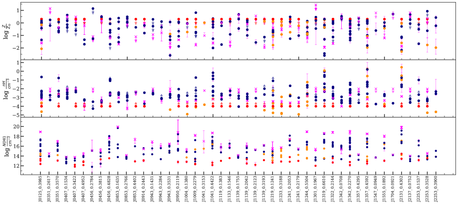
To compare the P19 results with the CMBM method, we show the derived metallicities, densities, and $N({\mbox{H\,{\sc i}}})$ for the different clouds along each sightline in Fig. 15. The single-valued properties or limits derived for each system by Pointon et al. (2019) are shown as a magenta cross. A typical sightline through a galaxy has several clouds in PIE and one TDP–High cloud, and perhaps half also have one or more TDP–Low clouds. The ranges of metallicities and densities can be up to two orders of magnitude along a single galaxy sightline. This reflects the fact that most sightlines pass through different parts of a galaxy, potentially having contributions in absorption from outer disk, halo, outflows, recycled accretion, tidal streams, satellite galaxies, etc. The single average metallicities are not systematically larger or smaller than the range of multi-cloud modelling results, showing that the situation is complicated, but that the single average value is not particularly representative of any of the gas clouds. The total system $N({\mbox{H\,{\sc i}}})$ values from P19 are often consistent with the value for the highest $N({\mbox{H\,{\sc i}}})$ cloud in the system using CMBM. The main cause for the differences in derived metallicities between our approach and P19 is that it is not typical for all of the H i to be associated with all of the metal line column.

Even with the detailed cloud information about multiple phases, there is still no indication of a relationship between azimuthal angle and metallicity as seen in Figs 13 and 14. There is no apparent trend for the highest or for the lowest metallicity cloud in a system, nor is there a trend for galaxies’ near-edge-on inclinations, where the largest difference between the major and minor axis is expected. Both high and low metallicity clouds are found along the same sightlines. To investigate this further, we chose a subsample of sightlines most likely to show differences between major and minor axes ( $\log N(\mbox{H\,{\sc i}})$ $\geq$ 15.0, inclination angle $\geq$ 60^∘, and impact parameter $\leq R_{\_}{\rm vir}$ ). A plot of the metallicity vs. azimuthal angle for the subsample, comprising of PIE and TDP–Low clouds, is shown in Fig. 16. There are very few sightlines close to the major axis that satisfy all the subsample criteria, but it is worth noting that the full range of metallicities is apparent along the minor axis, including high values expected for outflow clouds, as well as lower values that could be contributed by dwarf satellites and their stripped material. The simplest interpretation is that the gas in these $z<0.7$ galaxies is often well mixed, meaning that gas originating from different processes is now located in various parts of the galaxy.

A substantial insight into that interpretation is provided by the results of the FIRE–2 simulations (Hafen et al., 2019). The trajectories of different particles, characterized by their origins in IGM accretion, winds, or satellite winds, were followed for the 1 Gyr prior to $z=0.25$ for galaxy halos of mass $10^{12}$ M ${}_{\_}{\odot}$ , $10^{11}$ M ${}_{\_}{\odot}$ , and $10^{10}$ M ${}_{\_}{\odot}$ . The higher mass halos correspond to those in our present sample. The gas of different origins in the $10^{12}$ M ${}_{\_}{\odot}$ halos appears to be relatively well mixed at $z=0.25$ , with all three particle origins seen over the full halo volume. When only particles which originated recently, between 1 Gyr and 0.5 Gyr ago, are considered, we do see specific regions that the three types of particles prefer. The wind particles are close to the central galaxy, the satellite wind particles are mostly associated with three halo substructures and the accretion avoids some directions in the halo. When origins at all times are included, however, this asymmetry is no longer apparent. In conclusion, based on the results of Hafen et al. (2019), we should not have expected a relationship between metallicity and azimuthal angle in our sample. Gas at $z=0.25$ is well mixed, with gas from several origins present at all impact parameters and azimuthal angles.

At higher redshifts the contribution of outflows is larger (e.g., Muratov et al. 2015; Mitchell et al. 2018), and it is more likely that their signatures will be observable in absorption. Hafen et al. (2019) found that winds provided more than 40% of the inner halo mass at $z=2$ , and that the contributions of winds, satellite winds, and IGM accretion are all quite inhomogeneous and not well mixed. Thus if we were to perform this same experiment at high redshift we would be more likely to see relationships between azimuthal angle and metallicity for some of the clouds.

Though we did not see any trends of cloud properties with galaxy properties, we should note that the galaxies in our sample are relatively isolated, with no neighbors within 100 kpc and 500 km s^-1. This would imply fewer active interactions in these galaxies and less wind activity than for a more crowded environment (P19).

6.2 Nature and Origin of Different Cloud Types

In this section, we discuss the nature and origin of different types of clouds. One key principle to keep in mind is that every location along a sightline has a specific density, temperature, and metallicity. It is also important to note that together the thicknesses that we have derived for the clouds must sum to something of order a halo size or less.

In Fig. 4a, the three types of clouds found in our modelling, with the blue symbols representing cooler clouds in thermal equilibrium, the gold ones representing clouds of intermediate temperature that are modelled with time-dependent photoionization, and the red ones with detected O vi as hotter clouds also modelled with time-dependent photoionization, but as we discuss below, they are found to be in collisional ionization equilibrium.

6.2.1 PIE Clouds

First, we will discuss the PIE clouds. Fig. 6 showed that the majority of them have densities between $-3.5\leq$ $\log n_{\hbox{{\rm H}}}/\hbox{cm${}^{-3}$}$ $\leq-2.5$ , metallicities greater than solar, and small thicknesses less than a kpc and even sometimes sub-parsec. Werk et al. (2013) argued that the large scatter in the low-ion absorption strengths indicates that the cool CGM is patchy and hence reveals a wide range of ionization conditions. Many of the PIE clouds have weak, low ionization absorption detected, and their properties thus coincide with the metal-rich weak Mg ii absorbers studied by Rigby et al. (2002), Narayanan et al. (2005), and Muzahid et al. (2018). While it is tempting to characterize this population of absorbers as having a single origin, we must remember that gas of density $\log n_{\rm H}$ = $-3$ is surely not rare in galaxies and will occur in disk material, in outflows, in tidal debris, and in various other regions of the CGM. This population is common, with a typical sightline passing through a few of them (see Fig. 15).

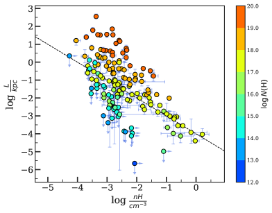
Theoretical arguments predict small, cold clouds in the CGM of galaxies in several contexts. McCourt et al. (2018) describe a hydrodynamic process by which cold gas fragments into a collection of smaller cloudlets by the process of cloud shattering, achieving equilibrium in the process. They predict that cold gas fragments down to a lengthscale given by $L=0.1$ pc/ $n_{\_}{\rm H}$ , with individual cloudlets having a characteristic column density $N_{\_}{cloudlet}$ $\sim$ 10¹⁷ cm^-2. This relationship is shown as a dashed line on the plot of $\log L$ vs. $\log n_{\_}H$ in Fig. 17. We find that the line is consistent with being a lower bound in PIE cloud thickness at every $\log n_{\rm H}$ , and the column densities of several of the PIE clouds are in remarkable agreement with $N_{\_}{\rm H}$ $\sim$ 10¹⁷ cm^-2, suggesting that fragmentation plays a role in their origin.

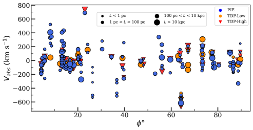
Several high-resolution numerical simulations also show small structures pervasive in the CGM. For example, the Mg ii column density distribution in the TNG50 simulation of Nelson et al. (2020) forms, through thermal instability, tens of thousands of fragments that are each a few 100 parsecs in size. Schneider et al. (2020) find many small fragments in the Cholla Outflow Simulation, which has a cell size of 5 pc. The expected CGM can be characterized as a galactic mist, with fragments from a larger cloud that are moving through a hot halo (Gronke & Oh, 2020). The fragments/droplets are not stable, but the larger cloud continues to produce smaller ones so they are ubiquitous. We plot the cloud velocities seen along different sightlines in our sample in Fig. 18 as a function of the azimuthal angle; this figure shows that both larger clouds and several smaller clouds are present along the same sightline. The larger clouds are, however, not always consistent in velocity with the small ones, but this is to be expected that the parent cloud would not always be intercepted along the same line of sight.

The idea of a galactic mist is often connected to an origin in outflows, which at face value would predict higher metallicities along the minor axis. Since we do not see such a trend between azimuthal angle and metallicity in our sample, that might suggest galactic mist is not an important process. On the other hand, if mixing is efficient and clouds can survive, this would not be a concern. Furthermore, the idea of fragmentation of cooler clouds moving through a hot halo is more universal than the specific idea of galactic mist. The Milky Way Galaxy does not have active outflows on large scales (Fox et al., 2019), but it does have a hot halo and multiphase high-velocity clouds passing through the halo. This could lead to fragmentation and the type of PIE clouds we are observing in these absorption systems.

6.2.2 TDP–Low Clouds

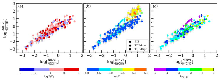
The TDP–Low clouds have considerable overlap with PIE clouds in the phase space of metallicity, density, and temperature. It is interesting to consider in what way they are out of thermal equilibrium in order to gain insight into their origins. Roughly half of the TDP–Low clouds have temperatures $4.7\lesssim$ $\log T/K$ $\lesssim 5.1$ , overlapping with PIE clouds but on the higher side, and metallicities $-2<$ $\log Z/Z_{\sun}$ $<0$ , also consistent with PIE clouds. This can be seen in Fig. 4. The biggest difference between these TDP–Low clouds, with higher temperatures, and the PIE clouds is that the densities of many of these TDP–Low clouds are the lowest of clouds in our sample, only $-5<$ $\log n_{\rm H}$ $<-4$ (see Fig. 5b). These densities correspond to large cloud thicknesses, in the range $10$ – $100$ kpc, among the largest in our sample (see Fig. 6). The Doppler parameters tend to be higher than those of the PIE sample because of higher temperatures (see Fig. 4 and 5). These larger Doppler parameters were constrained in our modelling process by the relative widths of lines from different ions. Perhaps the higher temperatures are responsible for the non-equilibrium conditions.

In Fig. 19, we use the line of ratios of key intermediate and high ionization transitions as another way to distinguish the TDP–Low clouds from the PIE clouds. Most of the TDP–Low clouds have $\log$ (O vi/C iii) ratio $\sim 0.5$ – $1$ dex higher than the PIE clouds on a plot of $\log$ (O vi/C iii) vs. $\log$ (N v/C iii). Fig. 19c shows that the TDP–Low clouds with the largest column densities of N v and O vi have the lowest densities, $\log n_{\rm H}$ $<-4$ , lower than any other clouds in our sample. For such low-density clouds, the time to achieve collisional ionization equilibrium is longer, and this gives rise to the need for TDP. This same low-density TDP–Low population includes those clouds with the highest temperatures among the TDP–Low clouds, in the interval $4.7\lesssim$ $\log T/K$ $\lesssim 5.1$ . Especially at these intermediate temperatures, cooling occurs rapidly, often without sufficient time to attain equilibrium. The other TDP–Low clouds have temperatures similar to PIE clouds, which implies some of them may be in or close to PIE. They were modelled with TDP only because they had detected C iv, but we found that in many of them the temperature needed to produce observed line ratios turned out to be consistent with equilibrium conditions.

6.2.3 TDP–High Clouds

The TDP–High clouds are distinguished from the other classes by their broad O vi profiles and higher derived temperatures in the range $5.5<$ $\log T$ $<6.0$ . In a few clouds, a discernable contribution to the Ly $\alpha$ profile is seen, but in most, the contribution to Ly $\alpha$ is negligible or dominated by other clouds in a saturated velocity range. The metallicities, densities, and sizes of these clouds are not constrained, as we discuss below.

Though our models allowed for non-equilibrium collisional ionization and for contributions from time-dependent photoionization, most of these O vi clouds are in collisional ionization equilibrium. In order to have a departure from equilibrium, the collisional ionization time scale would have to be short compared with the timescale for recombination. The resulting non-equilibrium, “overionized” condition occurs only for low densities, $\log n_{\rm H}$ $<-4$ for collisional ionization timescales longer than 10 million years (Oppenheimer & Schaye, 2013). In Fig. 1, we show that the ionization fraction of O vi diverges from the CIE expectation only at $\log T$ $\lesssim 5.2$ , and especially for high metallicities ( $Z/Z_{\_}{\odot}>1$ ). At those lower temperatures, the cooling times are short enough to leave the gas “overionized”. In Fig. 19b, we see that O vi/C iii for the TDP–High clouds is elevated by roughly an order of magnitude over the values for PIE clouds with the same large values of N v/C iii. This is also consistent with the origin of O vi in collisionally ionized material at a higher temperature.

In the absence of constraints on cloud sizes, an important question is whether the collisionally ionized O vi absorbing gas found through the TDP–High clouds is characteristic of the entire galaxy halo or whether this O vi arises in substructures within the halo. Such substructures could be small regions, heated by local processes, or could occupy a larger fraction of the halo (i.e., tens to 100 kpc). To understand the origin of these higher temperature regions giving rise to the TDP–High clouds, we can compare to numerical simulations and to known structures in the Milky Way galaxy and local universe.

Fig. 2 in Hafen et al. (2023) shows the temperature-vs-density distribution of CGM gas in FIRE-2 cosmological simulations of Milky Way-like galaxies. A substantial phase space density is present at the temperatures found for the collisionally ionized O vi clouds, and these clouds are at over an order of magnitude higher temperatures than given by the balance of heating and cooling. Appleby et al. (2023) have studied the physical conditions of CGM gas at low redshift using the SIMBA simulation Davé et al. (2019). They find that O vi absorbers arise in gas with a temperature distribution that peaks at $\log(T/{\rm K})=5.5$ , with at least 80% collisionally ionized, though there is a tail to lower temperatures with an origin in photoionized gas. They find that the majority of the O vi absorption arises from the inner CGM and characterize it as arising in WHIM or hot halo gas. This would imply larger, more diffuse structures.

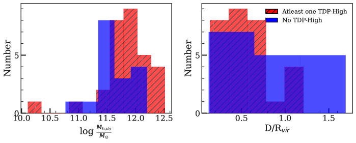
A favoured temperature for the presence of O vi absorption predicts a dependence of O vi on halo mass, as seen in a version of the eagle simulations that includes non-equilibrium ionization (Oppenheimer et al., 2016). These simulations show maximum O vi column densities for $L^{\star}$ galaxies with halo mass around $10^{12}$ M_⊙. More massive galaxies or groups have higher virial temperatures which promotes much of the oxygen to O vii and O viii. This halo mass preference for O vi absorption is seen observationally in the analyses of Pointon et al. (2017) and Ng et al. (2019), which compare galaxy properties to the measured column densities of O vi. (Nielsen et al., 2017; Kacprzak et al., 2019) also confirm that there are no obvious kinematic signatures in the O vi profiles that would signal contributions of outflow, inflow, or co-rotation. This is consistent with O vi arising in gas distributed over much of the galaxy halo.

We can more definitively confirm the presence of O vi halos around $L^{\star}$ galaxies by examining the galaxy properties for TDP–High clouds in our sample. Fig. 20a compares the mass distributions for sightlines through the 30 galaxies with one or more TDP–High cloud to the 17 sightlines through galaxies that have no detected TDP–High absorption. The interquartile range for the mass of galaxies without any TDP–High cloud is $\log M_{\_}{\rm halo}/M_{\_}{\odot}=11.4-11.9$ , lower than the range of 11.7–12.1 for galaxies with at least one TDP–High cloud. We perform a 2-sample Anderson-Darling test to test the null hypothesis that the galaxies with detected TDP–High absorption and the galaxies without detected TDP–High absorption are drawn from the same population. We find that the null hypothesis can be rejected at the 5% level ( $p=0.022$ ). Fig. 20 (b) shows the distributions of impact parameters comparing galaxies with at least one TDP–High cloud to galaxies without TDP–High clouds. We find that these two samples are also significantly different from one another ( $p=0.038$ ). This shows that several of the sightlines without TDP–High clouds are passing outside of the virial radius of their galaxies. We conclude that it is more likely for isolated, low redshift, more massive ( $\sim L^{\star}$ ) galaxies to be surrounded by collisionally ionized O vi halos extending to $0.6$ – $1.2$ virial radii.

Using semi-analytic models, Richter (2020) explored expectations for coronal broad Ly $\alpha$ lines from galaxy halos and predicted $\log(N({\mbox{H\,{\sc i}}})/{\rm cm}^{-2})=12.4-13.4$ and $b({\mbox{H\,{\sc i}}})$ of 70–200 km s^-1. Although the Ly $\alpha$ is not often detected because of the presence of other phases and the $S/N$ of the data, these values are consistent with the expectations for our TDP–High clouds (see Figs. 3a and 5a).

Within the coronal O vi halos of $L^{\star}$ galaxies, and in the lower mass galaxies in our sample, there can also be substructures that produce O vi absorption. In the specialized simulations of Mandelker et al. (2020), the O vi absorption arises in the turbulent mixing layer formed as a cold filamentary stream falls through the hot CGM. In such cases, the O vi is thus arising in kpc-scale structures, and the surrounding medium is too hot to give rise to O vi absorption. These would be more analogous to the TDP–Low clouds in our sample, those with $\log(T/{\rm K})\sim 5$ (Fig. 4a), which have O vi along with lower ionization transitions due to over-ionization.

There is also evidence that the TDP–High clouds are large substructures within halos. They must be large because, for massive enough galaxies within $0.75R_{\_}{\rm vir}$ , the covering factor for TDP–High clouds is close to unity in our sample. In addition, we find that 15 of the 30 sightlines with one or more TDP–High clouds have two or more of these clouds along the sightline. So these galaxies, with multiple components, have kinematically distinct substructures within the hot halos that give rise to the broad O vi lines. In other cases, there could be kinematically overlapping substructures that produce the O vi absorption from different regions within the halo. Fundamentally, there are likely to be many segments of gas along the sightline through the whole halo, with relatively low densities and temperatures consistent with the virial temperature, that shape the TDP–High O vi profiles that we observe.

The most detailed view that we have of structures like those that may be responsible for the O vi clouds (TDP–High and TDP–Low) is in the Local Group. For example, Krishnarao et al. (2022) published a focused study of the corona of the Large Magellanic Cloud (LMC). Their analysis provides evidence for a $\log T$ $\sim 5.5$ corona around the LMC within the larger $\log T$ $\sim 6$ Milky Way corona. Cooler clouds ( $\log T$ $\sim 4$ ) lie within the LMC corona, and C iv and Si iv absorption is produced in interface layers between these cool clouds and the LMC corona. Generalizing those measurements of the LMC corona, there are likely to be many substructures in the CGM of the galaxies in our sample in the form of dwarf galaxies, and other infalling structures. There is also an extended O vi corona surrounding Milky Way (and Andromeda) analogues in the High-resolution Environmental Simulations of The Immediate Area (HESTIA) model, with predicted O vi similar to the galaxies in our sample Damle et al. (2022).

We conclude that the TDP–High clouds are collisionally ionized. They are prevalent in $\sim L^{\star}$ galaxies and absent in some of the lower-mass galaxies in our sample. Their temperatures are consistent with the virial temperature for these halos, and their kinematics are consistent with expectations for one or two substructures of order the halo size. Our CMBM analysis has made it possible to detect the diffuse halo of most isolated, low redshift galaxies, separating it from other phases through the broad O vi absorption that it produces.

7 CONCLUSION

We inferred CGM absorption properties of 47, $z<0.7$ , isolated galaxy-absorber pairs from the “Multiphase Galaxy Halos” Survey using a cloud-by-cloud multiphase Bayesian ionization modelling approach. The metallicity of the CGM was compared with intrinsic absorber properties, including neutral hydrogen column density, temperature, Doppler parameter, hydrogen number density, and inferred line of sight thickness. We then compared the metallicity of the CGM to galaxy properties such as the galaxy inclination, azimuthal angle, impact parameter, halo mass, colours, and redshift. The galaxy inclinations and azimuthal angles were obtained by modelling the galaxies in HST images with GIM2D by P19. Our main findings are summarized here:

1.

We identify three main populations of CGM absorbers based on the type of models needed to best explain the observed multiphase absorption. The 47 absorption systems are found to comprise 240 clouds. The temperature distribution of the 157 cool PIE clouds is right-skewed with a median of $T\sim$ 10^4.1 K and a tail extending to $T\sim$ 10⁵ K. The temperature distribution of the 35 warm-hot TDP–Low and 48 hotter TDP–High clouds appears to be flat between $T\sim$ 10^4.2-5.2 K) and ( $T\sim$ 10^5.4-6.0 K).
2.

The metallicity for the PIE clouds ranges between $-2.6\lesssim$ $\log Z/Z_{\sun}$ $\lesssim 0.8$ , with a median metallicity of $\log Z/Z_{\sun}$ = $-0.41\pm 0.09$ . The TDP–Low clouds show a median metallicity of $-0.59\pm 0.19$ , and their metallicity ranges between $-2.3\lesssim$ $\log Z/Z_{\sun}$ $\lesssim 0.2$ . The TDP–High clouds are found to be in CIE and thus have unconstrained metallicities.
3.

The H i column density range of cool clouds (PIE) spans several decades 11.8 $\lesssim$ $\log N(\mbox{H\,{\sc i}})$ $\lesssim 19.7$ , and decreases as the impact parameter increases. The H i column density of warm-hot (TDP–Low) clouds ranges between $12.8\lesssim$ $\log N(\mbox{H\,{\sc i}})$ $\lesssim 17.2$ , and the H i column density of hotter phases (TDP–High) ranges between $12.0\lesssim$ $\log N(\mbox{H\,{\sc i}})$ $\lesssim 15.2$ .
4.

The cool clouds are explained by models that assume photoionization equilibrium (PIE). In agreement with theoretical predictions, we find that some of the PIE clouds follow the $L=0.1$ pc/ $n_{\_}{\rm H}$ relationship, consistent with the expectation of characteristic size scale for clouds formed by the process of fragmentation.
5.

About half of the warm-hot clouds, referred to as TDP–Low clouds, are found to be affected by time-dependent photoionization. These clouds are different from PIE clouds in their large ratios (0.5 $-$ 1 dex higher) of $\log$ (O vi/C iii). The remaining TDP–Low clouds have properties similar to PIE clouds, and these clouds may be in or close to PIE.
6.

The hotter clouds, referred to as TDP–High clouds, are distinguished from other classes by their broad O vi profiles. Though our models allowed for non-equilibrium ionization, most of the O vi clouds are found to be close to collisional ionization equilibrium at temperatures consistent with the virial temperatures of their galaxy halos. The lowest mass galaxies and sightlines at high impact parameters do not produce TDP–High clouds, but the $T\sim$ 10^5.7 K gas that produces them is abundant in $L^{\star}$ galaxy halos.
7.

A bimodality is observed in the azimuthal distribution of the total number of clouds and mean number of clouds per absorption system. More clouds are seen along minor and major axes ( $\Phi\lesssim 22.5^{\circ}$ $\cup$ $\Phi\gtrsim 67.5^{\circ}$ ), compared with interjacent azimuthal angles ( $22.5^{\circ}\lesssim\Phi\lesssim 67.5^{\circ}$ ).
8.

The metallicity is not related to the azimuthal angle. Additionally, the inclination angle, impact parameter, $B-K$ colours, subpopulations of the H i column density, or the absorber velocities with respect to the galaxy central velocity, have no bearing on this connection. The lack of a link between CGM metallicity and azimuthal angle in this low-redshift study challenges a simple model of the CGM with outflows along the minor axis and inflows along the major axis. A variety of other processes (e.g., disk material and recycled accretion) are contributing and there has been time for mixing of the different cloud populations in these galaxies.

Acknowledgements

We thank Nicolas Lehner and Christopher Howk for helpful discussions during the course of this work. S, J.C.C, B.W, acknowledges the support for this work through the grant number HST-AR-16607. Computations for this research were performed on the Pennsylvania State University’s Institute for Computational and Data Sciences’ Roar supercomputer. The authors also acknowledge the Texas Advanced Computing Center (TACC) at The University of Texas at Austin for providing HPC resources that have contributed to the research results reported within this paper. Parts of this research were supported by the Australian Research Council Centre of Excellence for All Sky Astrophysics in 3 Dimensions (ASTRO 3D), through project number CE170100013. A.N acknowledges the support for this work through grant number EMR/2017/002531 from the Department of Science and Technology, Government of India. We are grateful to Gary Ferland and collaborators for developing the cloudy photoionization code. We also thank Orly Gnat for making the computational data on radiatively cooling models public. This research made use of Astropy, a community-developed core Python package for Astronomy (Astropy Collaboration et al., 2013), NumPy (Harris et al., 2020), matplotlib (Hunter, 2007), and SciPy (Virtanen et al., 2020). This research has made use of the HSLA database, developed and maintained at STScI, Baltimore, USA. Some of the data presented herein were obtained at the W. M. Keck Observatory, which is operated as a scientific partnership among the California Institute of Technology, the University of California and the National Aeronautics and Space Administration. Observations were supported by Swinburne Keck programs 2014A_W178E, 2014B_W018E, 2015_W018E and 2016A_W056E. The Observatory was made possible by the generous financial support of the W. M. Keck Foundation. The authors wish to recognize and acknowledge the very significant cultural role and reverence that the summit of Maunakea has always had within the indigenous Hawaiian community. We are most fortunate to have the opportunity to conduct observations from this mountain. This research has made use of the NASA/IPAC Extragalactic Database (NED), which is operated by the Jet Propulsion Laboratory, California Institute of Technology, under contract with NASA. We acknowledge the work of people involved in the design, construction and deployment of the COS on-board the Hubble Space Telescope, and thank all those who obtained data for the sight-lines studied in this paper. We thank KITP for hosting the Fundamentals of Gaseous Halos workshop (supported by the NSF under Grant No. NSF PHY-1748958) during which some of the ideas presented in this work were formulated.

Data Availability

The data underlying this article will be shared on reasonable request to the corresponding author.

References

Acharya & Khaire (2021) Acharya A., Khaire V., 2021, MNRAS,
Akritas et al. (1995) Akritas M. G., Murphy S. A., Lavalley M. P., 1995, Journal of the American Statistical Association, 90, 170
Anglés-Alcázar et al. (2017) Anglés-Alcázar D., Faucher-Giguère C.-A., Kereš D., Hopkins P. F., Quataert E., Murray N., 2017, MNRAS, 470, 4698
Appleby et al. (2023) Appleby S., Davé R., Sorini D., Cui W., Christiansen J., 2023, MNRAS, 519, 5514
Astropy Collaboration et al. (2013) Astropy Collaboration et al., 2013, A&A, 558, A33
Barber et al. (1996) Barber C. B., Dobkin D. P., Huhdanpaa H., 1996, ACM Trans. Math. Softw., 22, 469–483
Berg et al. (2023) Berg M. A., et al., 2023, ApJ, 944, 101
Bond et al. (2001) Bond N. A., Churchill C. W., Charlton J. C., Vogt S. S., 2001, ApJ, 562, 641
Bordoloi et al. (2011a) Bordoloi R., et al., 2011a, ApJ, 743, 10
Bordoloi et al. (2011b) Bordoloi R., et al., 2011b, ApJ, 743, 10
Bordoloi et al. (2014) Bordoloi R., et al., 2014, ApJ, 794, 130
Borthakur (2022) Borthakur S., 2022, ApJ, 924, 123
Borthakur et al. (2015) Borthakur S., et al., 2015, ApJ, 813, 46
Bouché et al. (2012) Bouché N., Hohensee W., Vargas R., Kacprzak G. G., Martin C. L., Cooke J., Churchill C. W., 2012, MNRAS, 426, 801
Bregman (1980) Bregman J. N., 1980, ApJ, 236, 577
Buchner (2014) Buchner J., 2014, arXiv e-prints, p. arXiv:1407.5459
Burchett et al. (2013) Burchett J. N., Tripp T. M., Werk J. K., Howk J. C., Prochaska J. X., Ford A. B., Davé R., 2013, ApJ, 779, L17
Cen & Ostriker (2006) Cen R., Ostriker J. P., 2006, ApJ, 650, 560
Charlton et al. (2000) Charlton J. C., Mellon R. R., Rigby J. R., Churchill C. W., 2000, ApJ, 545, 635
Charlton et al. (2003) Charlton J. C., Ding J., Zonak S. G., Churchill C. W., Bond N. A., Rigby J. R., 2003, ApJ, 589, 111
Chen & Mulchaey (2009) Chen H.-W., Mulchaey J. S., 2009, ApJ, 701, 1219
Chen et al. (2001) Chen H.-W., Lanzetta K. M., Webb J. K., 2001, ApJ, 556, 158
Chen et al. (2010) Chen H.-W., Wild V., Tinker J. L., Gauthier J.-R., Helsby J. E., Shectman S. A., Thompson I. B., 2010, ApJ, 724, L176
Chiappini et al. (1997) Chiappini C., Matteucci F., Gratton R., 1997, ApJ, 477, 765
Churchill & Charlton (1999) Churchill C. W., Charlton J. C., 1999, AJ, 118, 59
Churchill & Vogt (2001) Churchill C. W., Vogt S. S., 2001, AJ, 122, 679
Churchill et al. (2012) Churchill C. W., Kacprzak G. G., Steidel C. C., Spitler L. R., Holtzman J., Nielsen N. M., Trujillo-Gomez S., 2012, ApJ, 760, 68
Churchill et al. (2013) Churchill C. W., Trujillo-Gomez S., Nielsen N. M., Kacprzak G. G., 2013, ApJ, 779, 87
Churchill et al. (2015) Churchill C. W., Vander Vliet J. R., Trujillo-Gomez S., Kacprzak G. G., Klypin A., 2015, ApJ, 802, 10
Crighton et al. (2015) Crighton N. H. M., Hennawi J. F., Simcoe R. A., Cooksey K. L., Murphy M. T., Fumagalli M., Prochaska J. X., Shanks T., 2015, MNRAS, 446, 18
Curran et al. (2016) Curran S. J., Reeves S. N., Allison J. R., Sadler E. M., 2016, MNRAS, 459, 4136
Damle et al. (2022) Damle M., et al., 2022, Monthly Notices of the Royal Astronomical Society, 512, 3717
Danforth et al. (2010) Danforth C. W., Stocke J. T., Shull J. M., 2010, ApJ, 710, 613
Danovich et al. (2012) Danovich M., Dekel A., Hahn O., Teyssier R., 2012, MNRAS, 422, 1732
Danovich et al. (2015) Danovich M., Dekel A., Hahn O., Ceverino D., Primack J., 2015, MNRAS, 449, 2087
Davé et al. (2011a) Davé R., Oppenheimer B. D., Finlator K., 2011a, MNRAS, 415, 11
Davé et al. (2011b) Davé R., Finlator K., Oppenheimer B. D., 2011b, MNRAS, 416, 1354
Davé et al. (2012) Davé R., Finlator K., Oppenheimer B. D., 2012, MNRAS, 421, 98
Davé et al. (2019) Davé R., Anglés-Alcázar D., Narayanan D., Li Q., Rafieferantsoa M. H., Appleby S., 2019, MNRAS, 486, 2827
Dekel & Birnboim (2006) Dekel A., Birnboim Y., 2006, MNRAS, 368, 2
Dekel et al. (2009) Dekel A., et al., 2009, Nature, 457, 451
Dekker et al. (2000) Dekker H., D’Odorico S., Kaufer A., Delabre B., Kotzlowski H., 2000, in Iye M., Moorwood A. F., eds, Society of Photo-Optical Instrumentation Engineers (SPIE) Conference Series Vol. 4008, Optical and IR Telescope Instrumentation and Detectors. pp 534–545, doi:10.1117/12.395512
Ding et al. (2003a) Ding J., Charlton J. C., Bond N. A., Zonak S. G., Churchill C. W., 2003a, ApJ, 587, 551
Ding et al. (2003b) Ding J., Charlton J. C., Churchill C. W., Palma C., 2003b, ApJ, 590, 746
Ding et al. (2005) Ding J., Charlton J. C., Churchill C. W., 2005, ApJ, 621, 615
Draganova (2015) Draganova N., 2015, arXiv e-prints, p. arXiv:1511.04604
Dutta et al. (2021) Dutta R., et al., 2021, MNRAS, 508, 4573
Faucher-Giguère et al. (2011) Faucher-Giguère C.-A., Kereš D., Ma C.-P., 2011, MNRAS, 417, 2982
Fielding & Bryan (2022) Fielding D. B., Bryan G. L., 2022, ApJ, 924, 82
Ford et al. (2014) Ford A. B., Davé R., Oppenheimer B. D., Katz N., Kollmeier J. A., Thompson R., Weinberg D. H., 2014, MNRAS, 444, 1260
Fox et al. (2013) Fox A. J., et al., 2013, ApJ, 778, 187
Fox et al. (2019) Fox A. J., Richter P., Ashley T., Heckman T. M., Lehner N., Werk J. K., Bordoloi R., Peeples M. S., 2019, ApJ, 884, 53
Fumagalli et al. (2011) Fumagalli M., O’Meara J. M., Prochaska J. X., 2011, Science, 334, 1245
Gibson et al. (2022) Gibson J. L., Lehner N., Oppenheimer B. D., Howk J. C., Cooksey K. L., Fox A. J., 2022, arXiv e-prints, p. arXiv:2204.07586
Gnat (2017) Gnat O., 2017, ApJS, 228, 11
Gobat (2022) Gobat C., 2022, Asymmetric Uncertainty: Handling nonstandard numerical uncertainties, Astrophysics Source Code Library, record ascl:2208.005 (ascl:2208.005)
Grevesse et al. (2010) Grevesse N., Asplund M., Sauval A. J., Scott P., 2010, Ap&SS, 328, 179
Gronke & Oh (2020) Gronke M., Oh S. P., 2020, MNRAS, 494, L27
Haardt & Madau (2001) Haardt F., Madau P., 2001, in Neumann D. M., Tran J. T. V., eds, Clusters of Galaxies and the High Redshift Universe Observed in X-rays. p. 64 (arXiv:astro-ph/0106018), doi:10.48550/arXiv.astro-ph/0106018
Haardt & Madau (2012) Haardt F., Madau P., 2012, ApJ, 746, 125
Hafen et al. (2017) Hafen Z., et al., 2017, MNRAS, 469, 2292
Hafen et al. (2019) Hafen Z., et al., 2019, MNRAS, 488, 1248
Hafen et al. (2023) Hafen Z., et al., 2023, arXiv e-prints, p. arXiv:2305.01842
Haislmaier et al. (2021) Haislmaier K. J., Tripp T. M., Katz N., Prochaska J. X., Burchett J. N., O’Meara J. M., Werk J. K., 2021, MNRAS, 502, 4993
Harris et al. (2020) Harris C. R., et al., 2020, Nature, 585, 357
Hunter (2007) Hunter J. D., 2007, Computing in Science & Engineering, 9, 90
Johnson et al. (2013) Johnson S. D., Chen H.-W., Mulchaey J. S., 2013, MNRAS, 434, 1765
Johnson et al. (2015) Johnson S. D., Chen H.-W., Mulchaey J. S., 2015, MNRAS, 449, 3263
Johnson et al. (2017) Johnson S. D., Chen H.-W., Mulchaey J. S., Schaye J., Straka L. A., 2017, ApJ, 850, L10
Jones et al. (2010) Jones T. M., Misawa T., Charlton J. C., Mshar A. C., Ferland G. J., 2010, ApJ, 715, 1497
Kacprzak et al. (2008) Kacprzak G. G., Churchill C. W., Steidel C. C., Murphy M. T., 2008, AJ, 135, 922
Kacprzak et al. (2010) Kacprzak G. G., Murphy M. T., Churchill C. W., 2010, MNRAS, 406, 445
Kacprzak et al. (2011) Kacprzak G. G., Churchill C. W., Barton E. J., Cooke J., 2011, ApJ, 733, 105
Kacprzak et al. (2012a) Kacprzak G. G., Churchill C. W., Steidel C. C., Spitler L. R., Holtzman J. A., 2012a, MNRAS, 427, 3029
Kacprzak et al. (2012b) Kacprzak G. G., Churchill C. W., Nielsen N. M., 2012b, ApJ, 760, L7
Kacprzak et al. (2015a) Kacprzak G. G., Muzahid S., Churchill C. W., Nielsen N. M., Charlton J. C., 2015a, ApJ, 815, 22
Kacprzak et al. (2015b) Kacprzak G. G., Muzahid S., Churchill C. W., Nielsen N. M., Charlton J. C., 2015b, ApJ, 815, 22
Kacprzak et al. (2016) Kacprzak G. G., et al., 2016, ApJ, 826, L11
Kacprzak et al. (2019) Kacprzak G. G., Pointon S. K., Nielsen N. M., Churchill C. W., Muzahid S., Charlton J. C., 2019, ApJ, 886, 91
Keeney et al. (2017) Keeney B. A., et al., 2017, ApJS, 230, 6
Keeney et al. (2018) Keeney B. A., et al., 2018, ApJS, 237, 11
Kereš et al. (2005) Kereš D., Katz N., Weinberg D. H., Davé R., 2005, MNRAS, 363, 2
Khaire & Srianand (2015) Khaire V., Srianand R., 2015, ApJ, 805, 33
Khaire et al. (2019) Khaire V., et al., 2019, MNRAS, 486, 769
Knuth (2006) Knuth K. H., 2006, arXiv e-prints, p. physics/0605197
Krishnarao et al. (2022) Krishnarao D., et al., 2022, Nature, 609, 915
Krogager (2018) Krogager J.-K., 2018, arXiv e-prints, p. arXiv:1803.01187
Kulkarni et al. (2022) Kulkarni V. P., Bowen D. V., Straka L. A., York D. G., Gupta N., Noterdaeme P., Srianand R., 2022, ApJ, 929, 150
Lacki & Charlton (2010) Lacki B. C., Charlton J. C., 2010, MNRAS, 403, 1556
Lan & Mo (2018) Lan T.-W., Mo H., 2018, ApJ, 866, 36
Lanzetta et al. (1995) Lanzetta K. M., Bowen D. V., Tytler D., Webb J. K., 1995, ApJ, 442, 538
Lehner et al. (2018) Lehner N., Wotta C. B., Howk J. C., O’Meara J. M., Oppenheimer B. D., Cooksey K. L., 2018, ApJ, 866, 33
Lehner et al. (2019) Lehner N., Wotta C. B., Howk J. C., O’Meara J. M., Oppenheimer B. D., Cooksey K. L., 2019, ApJ, 887, 5
Lehner et al. (2020) Lehner N., et al., 2020, ApJ, 900, 9
Lehner et al. (2022) Lehner N., et al., 2022, ApJ, 936, 156
Lochhaas et al. (2020) Lochhaas C., Bryan G. L., Li Y., Li M., Fielding D., 2020, MNRAS, 493, 1461
Lundgren et al. (2021) Lundgren B. F., et al., 2021, ApJ, 913, 50
Lynch & Charlton (2007) Lynch R. S., Charlton J. C., 2007, ApJ, 666, 64
Maller & Bullock (2004) Maller A. H., Bullock J. S., 2004, MNRAS, 355, 694
Mandelker et al. (2020) Mandelker N., van den Bosch F. C., Nagai D., Dekel A., Birnboim Y., Aung H., 2020, MNRAS, 498, 2415
Marra et al. (2021) Marra R., et al., 2021, MNRAS, 508, 4938
Marra et al. (2022) Marra R., Churchill C. W., Kacprzak G. G., Nielsen N. M., Trujillo-Gomez S., Lewis E., 2022, arXiv e-prints, p. arXiv:2202.12228
Martin et al. (2019) Martin C. L., Ho S. H., Kacprzak G. G., Churchill C. W., 2019, ApJ, 878, 84
Masiero et al. (2005) Masiero J. R., Charlton J. C., Ding J., Churchill C. W., Kacprzak G., 2005, ApJ, 623, 57
Mathes et al. (2014) Mathes N. L., Churchill C. W., Kacprzak G. G., Nielsen N. M., Trujillo-Gomez S., Charlton J., Muzahid S., 2014, ApJ, 792, 128
McCourt et al. (2018) McCourt M., Oh S. P., O’Leary R., Madigan A.-M., 2018, MNRAS, 473, 5407
Meiring et al. (2011) Meiring J. D., et al., 2011, ApJ, 732, 35
Misawa et al. (2008) Misawa T., Charlton J. C., Narayanan A., 2008, ApJ, 679, 220
Mitchell et al. (2018) Mitchell P. D., Blaizot J., Devriendt J., Kimm T., Michel-Dansac L., Rosdahl J., Slyz A., 2018, MNRAS, 474, 4279
Muratov et al. (2015) Muratov A. L., Kereš D., Faucher-Giguère C.-A., Hopkins P. F., Quataert E., Murray N., 2015, MNRAS, 454, 2691
Murphy (2016) Murphy M., 2016, Uves_Popler: Uves_Popler: Post-Pipeline Echelle Reduction Software, doi:10.5281/zenodo.56158
Murphy et al. (2019) Murphy M. T., Kacprzak G. G., Savorgnan G. A. D., Carswell R. F., 2019, MNRAS, 482, 3458
Muzahid et al. (2015) Muzahid S., Kacprzak G. G., Churchill C. W., Charlton J. C., Nielsen N. M., Mathes N. L., Trujillo-Gomez S., 2015, ApJ, 811, 132
Muzahid et al. (2016) Muzahid S., Kacprzak G. G., Charlton J. C., Churchill C. W., 2016, ApJ, 823, 66
Muzahid et al. (2018) Muzahid S., Fonseca G., Roberts A., Rosenwasser B., Richter P., Narayanan A., Churchill C., Charlton J., 2018, MNRAS, 476, 4965
Narayanan et al. (2005) Narayanan A., Charlton J. C., Masiero J. R., Lynch R., 2005, ApJ, 632, 92
Narayanan et al. (2010) Narayanan A., Savage B. D., Wakker B. P., 2010, ApJ, 712, 1443
Narayanan et al. (2011) Narayanan A., et al., 2011, ApJ, 730, 15
Narayanan et al. (2012) Narayanan A., Savage B. D., Wakker B. P., 2012, ApJ, 752, 65
Narayanan et al. (2021) Narayanan A., et al., 2021, MNRAS, 505, 738
Nateghi et al. (2021) Nateghi H., Kacprzak G. G., Nielsen N. M., Muzahid S., Churchill C. W., Pointon S. K., Charlton J. C., 2021, MNRAS, 500, 3987
Nateghi et al. (2023) Nateghi H., Kacprzak G. G., Nielsen N. M., Murphy M. T., Churchill C. W., Muzahid S., Sameer and Charlton J. C., 2023, MNRAS, Submitted
Navarro et al. (1996) Navarro J. F., Frenk C. S., White S. D. M., 1996, ApJ, 462, 563
Nelson et al. (2018) Nelson D., et al., 2018, MNRAS, 477, 450
Nelson et al. (2019) Nelson D., et al., 2019, MNRAS, 490, 3234
Nelson et al. (2020) Nelson D., et al., 2020, MNRAS, 498, 2391
Ng et al. (2019) Ng M., Nielsen N. M., Kacprzak G. G., Pointon S. K., Muzahid S., Churchill C. W., Charlton J. C., 2019, ApJ, 886, 66
Nielsen et al. (2013a) Nielsen N. M., Churchill C. W., Kacprzak G. G., Murphy M. T., 2013a, ApJ, 776, 114
Nielsen et al. (2013b) Nielsen N. M., Churchill C. W., Kacprzak G. G., 2013b, ApJ, 776, 115
Nielsen et al. (2017) Nielsen N. M., Kacprzak G. G., Muzahid S., Churchill C. W., Murphy M. T., Charlton J. C., 2017, ApJ, 834, 148
Nielsen et al. (2022) Nielsen N. M., Kacprzak G. G., Sameer Murphy M. T., Nateghi H., Charlton J. C., Churchill C. W., 2022, MNRAS, 514, 6074
Norris et al. (2021) Norris J. M., Muzahid S., Charlton J. C., Kacprzak G. G., Wakker B. P., Churchill C. W., 2021, MNRAS, 506, 5640
Oort (1970) Oort J. H., 1970, A&A, 7, 381
Oppenheimer & Schaye (2013) Oppenheimer B. D., Schaye J., 2013, MNRAS, 434, 1063
Oppenheimer et al. (2010) Oppenheimer B. D., Davé R., Kereš D., Fardal M., Katz N., Kollmeier J. A., Weinberg D. H., 2010, MNRAS, 406, 2325
Oppenheimer et al. (2012) Oppenheimer B. D., Davé R., Katz N., Kollmeier J. A., Weinberg D. H., 2012, MNRAS, 420, 829
Oppenheimer et al. (2016) Oppenheimer B. D., et al., 2016, MNRAS, 460, 2157
Pagel (1989) Pagel B. E. J., 1989, in Beckman J. E., Pagel B. E. J., eds, Evolutionary Phenomena in Galaxies. p. 201
Pagel & Patchett (1975) Pagel B. E. J., Patchett B. E., 1975, MNRAS, 172, 13
Pandya et al. (2020) Pandya V., et al., 2020, ApJ, 905, 4
Pandya et al. (2021) Pandya V., et al., 2021, MNRAS, 508, 2979
Peeples et al. (2019) Peeples M. S., et al., 2019, ApJ, 873, 129
Péroux et al. (2020) Péroux C., Nelson D., van de Voort F., Pillepich A., Marinacci F., Vogelsberger M., Hernquist L., 2020, MNRAS, 499, 2462
Peterson et al. (1998) Peterson B. M., Wanders I., Bertram R., Hunley J. F., Pogge R. W., Wagner R. M., 1998, ApJ, 501, 82
Pillepich et al. (2019) Pillepich A., et al., 2019, MNRAS, 490, 3196
Pointon et al. (2017) Pointon S. K., Nielsen N. M., Kacprzak G. G., Muzahid S., Churchill C. W., Charlton J. C., 2017, ApJ, 844, 23
Pointon et al. (2019) Pointon S. K., Kacprzak G. G., Nielsen N. M., Muzahid S., Murphy M. T., Churchill C. W., Charlton J. C., 2019, ApJ, 883, 78
Prochaska et al. (2011) Prochaska J. X., Weiner B., Chen H. W., Mulchaey J., Cooksey K., 2011, ApJ, 740, 91
Prochaska et al. (2017) Prochaska J. X., et al., 2017, ApJ, 837, 169
Rao et al. (2011) Rao S. M., Belfort-Mihalyi M., Turnshek D. A., Monier E. M., Nestor D. B., Quider A., 2011, MNRAS, 416, 1215
Rauch et al. (2002) Rauch M., Sargent W. L. W., Barlow T. A., Simcoe R. A., 2002, ApJ, 576, 45
Richter (2020) Richter P., 2020, ApJ, 892, 33
Richter et al. (2011) Richter P., Krause F., Fechner C., Charlton J. C., Murphy M. T., 2011, A&A, 528, A12
Richter et al. (2018) Richter P., et al., 2018, ApJ, 868, 112
Rigby et al. (2002) Rigby J. R., Charlton J. C., Churchill C. W., 2002, ApJ, 565, 743
Robertson et al. (1988) Robertson J. G., Morton D. C., Blades J. C., York D. G., Meyer D. M., 1988, ApJ, 325, 635
Rosenwasser et al. (2018) Rosenwasser B., Muzahid S., Charlton J. C., Kacprzak G. G., Wakker B. P., Churchill C. W., 2018, MNRAS, 476, 2258
Rubin et al. (2012) Rubin K. H. R., Prochaska J. X., Koo D. C., Phillips A. C., 2012, ApJ, 747, L26
Rubin et al. (2014) Rubin K. H. R., Prochaska J. X., Koo D. C., Phillips A. C., Martin C. L., Winstrom L. O., 2014, ApJ, 794, 156
Rudie et al. (2012) Rudie G. C., et al., 2012, ApJ, 750, 67
Sameer et al. (2021) Sameer et al., 2021, MNRAS, 501, 2112
Sameer et al. (2022) Sameer et al., 2022, MNRAS, 510, 5796
Savage et al. (2010) Savage B. D., et al., 2010, ApJ, 719, 1526
Savage et al. (2011a) Savage B. D., Narayanan A., Lehner N., Wakker B. P., 2011a, ApJ, 731, 14
Savage et al. (2011b) Savage B. D., Lehner N., Narayanan A., 2011b, ApJ, 743, 180
Savage et al. (2014) Savage B. D., Kim T. S., Wakker B. P., Keeney B., Shull J. M., Stocke J. T., Green J. C., 2014, ApJS, 212, 8
Schneider (2006) Schneider P., 2006, Extragalactic astronomy and cosmology: an introduction. Vol. 146, Springer
Schneider et al. (2020) Schneider E. E., Ostriker E. C., Robertson B. E., Thompson T. A., 2020, ApJ, 895, 43
Scholz & Stephens (1987) Scholz F. W., Stephens M. A., 1987, Journal of the American Statistical Association, 82, 918
Shapiro & Field (1976) Shapiro P. R., Field G. B., 1976, ApJ, 205, 762
Shen et al. (2013) Shen S., Madau P., Guedes J., Mayer L., Prochaska J. X., Wadsley J., 2013, ApJ, 765, 89
Shull et al. (2012) Shull J. M., Stevans M., Danforth C. W., 2012, ApJ, 752, 162
Springel & Hernquist (2003) Springel V., Hernquist L., 2003, MNRAS, 339, 289
Steidel et al. (2010) Steidel C. C., Erb D. K., Shapley A. E., Pettini M., Reddy N., Bogosavljević M., Rudie G. C., Rakic O., 2010, ApJ, 717, 289
Stewart et al. (2011) Stewart K. R., Kaufmann T., Bullock J. S., Barton E. J., Maller A. H., Diemand J., Wadsley J., 2011, ApJ, 738, 39
Stewart et al. (2013) Stewart K. R., Brooks A. M., Bullock J. S., Maller A. H., Diemand J., Wadsley J., Moustakas L. A., 2013, ApJ, 769, 74
Stewart et al. (2017) Stewart K. R., et al., 2017, ApJ, 843, 47
Tepper-García (2006) Tepper-García T., 2006, MNRAS, 369, 2025
Tilton & Shull (2013) Tilton E. M., Shull J. M., 2013, ApJ, 774, 67
Tilton et al. (2012) Tilton E. M., Danforth C. W., Shull J. M., Ross T. L., 2012, ApJ, 759, 112
Tripp et al. (1998) Tripp T. M., Lu L., Savage B. D., 1998, ApJ, 508, 200
Tripp et al. (2001) Tripp T. M., Giroux M. L., Stocke J. T., Tumlinson J., Oegerle W. R., 2001, ApJ, 563, 724
Tripp et al. (2011) Tripp T. M., et al., 2011, Science, 334, 952
Tumlinson et al. (2011a) Tumlinson J., et al., 2011a, Science, 334, 948
Tumlinson et al. (2011b) Tumlinson J., et al., 2011b, Science, 334, 948
Tumlinson et al. (2017) Tumlinson J., Peeples M. S., Werk J. K., 2017, ARA&A, 55, 389
Veilleux et al. (2005) Veilleux S., Cecil G., Bland-Hawthorn J., 2005, ARA&A, 43, 769
Virtanen et al. (2020) Virtanen P., et al., 2020, scipy/scipy: SciPy 1.5.3, doi:10.5281/zenodo.4100507
Wakker (2006) Wakker B. P., 2006, ApJS, 163, 282
Wakker & Savage (2009) Wakker B. P., Savage B. D., 2009, ApJS, 182, 378
Wakker & van Woerden (1997) Wakker B. P., van Woerden H., 1997, ARA&A, 35, 217
Wakker et al. (1999) Wakker B. P., et al., 1999, Nature, 402, 388
Wakker et al. (2015) Wakker B. P., Hernandez A. K., French D. M., Kim T.-S., Oppenheimer B. D., Savage B. D., 2015, ApJ, 814, 40
Wendt et al. (2021) Wendt M., Bouché N. F., Zabl J., Schroetter I., Muzahid S., 2021, MNRAS, 502, 3733
Werk et al. (2012) Werk J. K., Prochaska J. X., Thom C., Tumlinson J., Tripp T. M., O’Meara J. M., Meiring J. D., 2012, ApJS, 198, 3
Werk et al. (2013) Werk J. K., Prochaska J. X., Thom C., Tumlinson J., Tripp T. M., O’Meara J. M., Peeples M. S., 2013, ApJS, 204, 17
Werk et al. (2014) Werk J. K., et al., 2014, ApJ, 792, 8
Werk et al. (2016) Werk J. K., et al., 2016, ApJ, 833, 54
Wotta et al. (2019) Wotta C. B., Lehner N., Howk J. C., O’Meara J. M., Oppenheimer B. D., Cooksey K. L., 2019, ApJ, 872, 81
Yuan et al. (2002) Yuan Q., Green R. F., Brotherton M., Tripp T. M., Kaiser M. E., Kriss G. A., 2002, ApJ, 575, 687
Zahedy et al. (2019a) Zahedy F. S., Chen H.-W., Johnson S. D., Pierce R. M., Rauch M., Huang Y.-H., Weiner B. J., Gauthier J.-R., 2019a, MNRAS, 484, 2257
Zahedy et al. (2019b) Zahedy F. S., Chen H.-W., Johnson S. D., Pierce R. M., Rauch M., Huang Y.-H., Weiner B. J., Gauthier J.-R., 2019b, MNRAS, 484, 2257
Zheng et al. (2017) Zheng Y., Peek J. E. G., Werk J. K., Putman M. E., 2017, ApJ, 834, 179
Zonak et al. (2004) Zonak S. G., Charlton J. C., Ding J., Churchill C. W., 2004, ApJ, 606, 196
van de Voort & Schaye (2012) van de Voort F., Schaye J., 2012, MNRAS, 423, 2991
van den Bergh (1962) van den Bergh S., 1962, AJ, 67, 486

Appendix A Galaxy Observations and Properties

Table 3: Galaxy Observations and Properties

(1)

(2)

(3)

(4)

(5)

(6)

(7)

(8)

(9)

(10)

(11)

(12)

(13)

(14)

(15)

J-Name

Cross ID

z_{\_}{\rm gal}

Ref.^a

DEC

D

B-K

\Phi

i

\log M_{\_}{h}/M_{\_}{\odot}

R_{\rm vir}

D/R_{\_}{vir}

V_{\_}{c}(D)

\log{\rm sSFR}

, Galaxy Type, Reference

(J2000)

(kpc)

({{}^{\circ}})

({{}^{\circ}})

(kpc)

(km s^-1)

(yr^-1)

Columns (1): SDSS J-Name of the quasar, (2): Cross ID of the quasar, (3): Galaxy redshift, (4): Galaxy redshift reference: $(1)$ Kacprzak et al. (2019), $(2)$ Chen et al. (2001), $(3)$ Johnson et al. (2013), $(4)$ P19, $(5)$ Kacprzak et al. (2011), $(6)$ Werk et al. (2012), $(7)$ Lanzetta et al. (1995), $(8)$ Prochaska et al. (2011), $(9)$ Kacprzak et al. (2012a), (5) & (6): RA and DEC in SDSS J2000 equatorial coordinates for the quasar, (7): Impact parameter of the sightline, (8): Galaxy color in $B-K$ magnitude, (9): Azimuthal angle of the galaxy, $\phi$ = 0^∘ corresponds to the major axis of the galaxy. We note that the uncertainties in the azimuthal angles of face-on galaxies ( $i<20$ ^∘) are statistical errors derived from modelling in GIM2D. It is possible that the systematic errors are larger, (10): Inclination angle of the galaxy, $i$ = 0^∘ implies the galaxy is oriented face-on along our line of sight, (11): Halo mass of the galaxy in log units of solar mass, (12): Virial radius of the galaxy, (13): Impact parameter scaled by the virial radius, (14): Galaxy circular velocity measured at the impact parameter, (15): when available we give the $\log{\rm sSFR}$ , Galaxy Type, and reference for this information. For galaxy type, SF refers to a star-forming galaxy, and P refers to a passive galaxy. A galaxy is considered star-forming when its $\log{\rm sSFR}$ is $\geq-11$ (Tumlinson et al., 2011b). The references are MZ15 – Muzahid et al. (2015), J13 – Johnson et al. (2013), J15 – Johnson et al. (2015), J17 – Johnson et al. (2017), W13 – Werk et al. (2013), K17 – Keeney et al. (2017), K18 – Keeney et al. (2018), Z19 – Zahedy et al. (2019a). A portion of this table (columns 1, 3–11) is reproduced from P19 for the convenience of the reader.

Appendix B Notes on Ionization Modelling

B.1 Table of Cloud-by-cloud properties of the absorption systems

Table 4: Cloud-by-cloud properties of the absorption systems

(1)	(2)	(3)	(4)	(5)	(6)	(7)	(8)	(9)	(10)	(11)	(12)	(13)
J-Name	$z_{\_}{\rm gal}$	$V$	$\log Z/Z_{\sun}$	$\log n_{\hbox{{\rm H}}}/\hbox{cm${}^{-3}$}$	$\log N(\rm H)/\hbox{cm${}^{-2}$}$	$\log N(\mbox{H\,{\sc i}})/\hbox{cm${}^{-2}$}$	$\log T/K$	$\log L/kpc$	b_nT	b ${}_{\rm{T}}(\rm{\mbox{H\,{\sc i}}})$	b $(\rm{\mbox{H\,{\sc i}}})$	Ionization Model
		km s^-1							km s^-1	km s^-1	km s^-1

Properties of the different gas phases that contribute to the absorption towards different sightlines. Notes: (1) J-Name of the quasar; (2) Redshift of the galaxy; (3) Velocity of the cloud w.r.t the galaxy, sorted in increasing order; (4) cloud metallicity; (5) cloud total hydrogen volume density; (6) cloud total hydrogen column density; (7) cloud hydrogen column density; (8) cloud temperature; (9) cloud line of sight thickness; (10) cloud non-thermal Doppler broadening parameter (11) cloud thermal Doppler broadening parameter measured for H i; (12) cloud total Doppler broadening parameter measured for H i; (13) type of ionization model for the cloud; PIE - Photoionized Equilibrium, TDP - Time Dependent Photoionized (see Section 3.1). The marginalised posterior values of model parameters are given as the median along with the upper and lower bounds corresponding to the 16–84 percentiles. The lower and upper limits correspond to $\mu_{\_}{1/2}-2\sigma$ and $\mu_{\_}{1/2}+2\sigma$ , respectively.

B.2 The absorption associated with the z = 0.3985 galaxy towards the quasar J0125

A system plot of this absorber is presented in Fig. 21. This system shows absorption in the low ionization transitions of Si ii, Mg ii, C ii, and N ii, and the intermediate ionization transition of Si iii. We also see absorption in the higher ionization transitions of N v and O vi. The C iv and Si iv are covered by the G225M grating but do not provide very useful constraints because of the poor S/N of the data.

The C ii $\lambda$ 1036 is blended with N iv $\lambda$ 765 line of the $z\approx$ 0.8950 absorber at $\approx$ 150 km s^-1. The contributions of C ii $\lambda$ 1036 and O vi $\lambda$ 1037 to one another within this system are masked. The Si ii $\lambda$ 1190 is contaminated with Si iii of the $z\approx$ 0.3791 absorber at $\approx$ $-$ 160 km s^-1. The Si ii $\lambda$ 1193 is contaminated with Ly $\alpha$ of the $z\approx$ 0.3726 absorber at $\approx$ $-$ 25 km s^-1, and by the Galactic Al ii absorption between $\approx$ 200–300 km s^-1. The Si ii $\lambda$ 1260 is contaminated with O vi of the $z\approx$ 0.6981 absorber between $\approx$ $-$ 150 – $-$ 100 km s^-1, and with H i $\lambda$ 930 of the $z\approx$ 0.8950 absorber between $\approx$ 200 – 300 km s^-1. The N ii $\lambda$ 1083 is contaminated with Si iii of the $z\approx$ 0.2565 absorber at $\approx$ 0 km s^-1. The Si iv $\lambda$ 1393 is contaminated with Ly $\alpha$ of the $z\approx$ 0.6044 and 0.6048 absorbers between $\approx$ 150 – 350 km s^-1. The C iv $\lambda$ 1548 is contaminated with Ly $\alpha$ of the $z\approx$ 0.7797, 0.7802, 0.7813, and 0.7820 absorbers between $\approx$ $-$ 200 – 200 km s^-1. The C iv $\lambda$ 1550 is contaminated with Ly $\alpha$ of the $z\approx$ 0.7844 absorber at 150 km s^-1. The N v $\lambda$ 1238 is contaminated with Ly $\alpha$ of the $z\approx$ 0.4267 at $\approx$ 325 km s^-1. The N v $\lambda$ 1242 is contaminated with Si ii of the $z\approx$ 0.3791 absorber at $\approx$ 37 km s^-1, and by the Ly $\alpha$ of the $z\approx$ 0.4314 at $\approx$ 350 km s^-1.

The low ionization absorption traced by Mg ii resolves into three components at $\approx$ $-$ 10, 184, and 198 km s^-1 in the high-resolution UVES data. The cloud at $\approx$ $-$ 10 km s^-1 is a low metallicity cloud with $\log Z/Z_{\sun}$ $\approx$ $-$ 1.4 and a density of $\approx$ $-$ 2.4. The clouds at 190 km s^-1 and 200 km s^-1 have metallicities consistent with solar $\log Z/Z_{\sun}$ $\approx$ 0 and 0.15, respectively, but contrasting densities of $\log n_{\rm H}$ $\approx$ $-$ 0.6 and $-$ 2.3, respectively. The densities of these clouds are well constrained owing to coincident absorption seen in Mg i, N ii, C ii, Si ii, and Si iii, and the metallicities are constrained from the profile shapes of Ly $\beta$ and Ly $\alpha$ . The overproduction of absorption in Ca ii suggests depletion due to dust, however, it was not used as a constraint.

The clouds at $\approx$ $-$ 63 km s^-1 and $\approx$ 88 km s^-1 are found to probe intermediate ionization gas traced by Si iii. The former cloud is determined to have a metallicity $\log Z/Z_{\sun}$ $\approx$ $-$ 0.4 and a density $\log n_{\rm H}$ $\approx$ $-$ 2.8. The properties of this cloud are constrained by the non-detections in low ionization species and the profile shape of Ly $\beta$ . The latter cloud is determined to have a metallicity of $\log Z/Z_{\sun}$ $\approx$ 0 and a density $\log n_{\rm H}$ $\approx$ $-$ 2.6. There is also a cloud traced by the Si iii absorption at $\approx$ 216 km s^-1 with a metallicity, $\log Z/Z_{\sun}$ $\approx$ $-$ 0.4 and a density $\log n_{\rm H}$ $\approx$ $-$ 3.0. The metallicity of this cloud is constrained by the shape of the Ly $\beta$ profile, and its density is constrained by the ratio of Si ii and Si iii, and coincident non-detections of other low ionization species.

The higher ionization gas phase traced by the O vi absorption resolves into five components centred at $\approx$ $-$ 64 km s^-1, 5 km s^-1, 87 km s^-1, 198 km s^-1, and 307 km s^-1. The components at $-$ 64 km s^-1, 5 km s^-1, and 198 km s^-1 contribute as weak broad Ly $\alpha$ absorbers with temperatures between $\log T$ $\sim$ 5.5–5.8. The metallicities and densities of these clouds are unconstrained as indicated by their platykurtic posterior distributions. We adopt upper limits and lower limits for metallicity and density, and set them to the upper and lower bound of their priors, respectively. The O vi clouds at 87 km s^-1 and 307 km s^-1 are at relatively lower temperatures $\log T$ $\approx$ 5.2 and 4.6, respectively, owing to their narrow profile shape and also produce absorption seen in the noisy C iv profiles.

There is a Ly $\alpha$ -only cloud with no associated metals at $-$ 115 km s^-1. There properties of this cloud are not well constrained owing to the lack of detected metal absorption. We adopt an upper limit for its metallicity and a lower limit for its density.

B.3 The absorption associated with the z = 0.2617 galaxy towards the quasar J0351

A system plot of this absorber is presented in Fig. 22. This system does not show any metal line absorption except in C iii. We mainly see absorption in H i Ly $\alpha$ . The absorption in H i resolves into two components centred at $\approx$ $-91$ km s^-1 and $-46$ km s^-1. The Ly $\beta$ is contaminated by Si iii arising in the $z\approx$ 0.07192, 0.07218, and 0.07252 absorbers. The Ly $\gamma$ is also contaminated by C ii $\lambda$ 903.6 and $\lambda$ 903.9 arising in the $z\approx$ 0.35667 absorber. The C ii $\lambda$ 1334 line is blended with the Ly $\alpha$ absorber at $z\approx$ 0.38517 at $\approx$ 20 km s^-1.

The metallicity and density of these clouds are unconstrained due to the lack of metal line absorption. The H i column densities are relatively well constrained because of the access to unsaturated higher-order Lyman series lines.

B.4 The absorption associated with the z = 0.3570 galaxy towards the quasar J0351

A system plot of this absorber is presented in Fig. 23. This system shows absorption in the low ionization transitions of Mg ii, C ii, Si ii, and N ii, and in the intermediate ionization transition of Si iii. We also see absorption in the high ionization transitions of C iv, N v, and O vi.

The C ii $\lambda$ 903.9 line is presented, and is overlapping with the C ii $\lambda$ 903.6 line which is masked out. The C ii $\lambda$ 1036 line is contaminated by the C iii $\lambda$ 977 line from the $z\approx$ 0.43981 absorber at $\approx$ 100 km s^-1. The N iii $\lambda$ 989 line is overlapping with the Si iii $\lambda$ 989 at $\approx$ 70 km s^-1. N v $\lambda$ 1238 is contaminated by Ly $\alpha$ from the $z\approx$ 0.38212 absorber at $-$ 160 km s^-1. The O vi $\lambda$ 1031 line is contaminated with Ly $\gamma$ of the $z\approx$ 0.43981 absorber between $-$ 70 km s^-1 – 70 km s^-1. The Si ii $\lambda$ 1190 is contaminated with Ly $\alpha$ of the $z\approx$ 0.32849 absorber at $-$ 65 km s^-1.

The high resolution spectrum of Mg ii resolves into three components at $\approx$ $-$ 75 km s^-1, $-$ 13 km s^-1, and 40 km s^-1. The properties of the gas phases traced by these three Mg ii components are metallicities of $\log Z/Z_{\sun}$ $\approx$ 0, $-$ 0.6, and 0, and densities of $\log n_{\rm H}$ $\approx$ $-2.2$ , $-0.8$ , and $-2.9$ . These gas phases also explain all of the absorption seen in the Si ii, C ii, and some of the absorption in Si iv and C iv. The Lyman series constrains the metallicities of these phases, while the Si iii and other intermediate ionization states constrain the density of the gas. The strongest Si iii absorption seen at $-$ 26 km s^-1 is found to arise in a separate phase and is needed to fill in the absorption seen in higher order Lyman series. The properties of this gas phase are $\log Z/Z_{\sun}$ $\approx$ $-$ 0.7 and $\log n_{\rm H}$ $\approx$ $-$ 2.8. There is also some absorption seen in Si iii at $-$ 149 km s^-1 that is needed to explain the coincident absorption seen in the Lyman series with a metallicity, $\log Z/Z_{\sun}$ $\approx-0.4$ and density, $\log n_{\rm H}$ $\approx-2.6$ . The O vi at $\approx$ $-$ 48 km s^-1 is at a temperature of $\log T$ $\approx$ 5.1 and this gas phase also produces the absorption seen in C iv and N v at coincident velocities. The metallicity of this cloud is $\log Z/Z_{\sun}$ $\approx$ 0.2 and a density of $\log n_{\rm H}$ $\approx$ $-$ 2.7. The O vi at $\approx$ $-$ 7 km s^-1 produces weak broad absorption in Ly $\alpha$ ; this phase is at a higher temperature of $\log T$ $\approx$ 5.7, and both its metallicity and density are unconstrained.

B.5 The absorption associated with the z = 0.1534 galaxy towards the quasar J0407

A system plot of this absorber is presented in Fig. 24. We only see absorption in the Ly $\alpha$ and Ly $\beta$ lines, and do not see any metal line absorption. The absorption resolves into five Ly $\alpha$ clouds. The metallicity and density are not constrained for these clouds, and we adopt upper limits and lower limits, respectively, for these parameters.

B.6 The absorption associated with the z = 0.3422 galaxy towards the quasar J0407

A system plot of this absorber is presented in Fig. 25. This absorption system does not show any absorption in the low or intermediate ionization species. We only see absorption in O vi, which resolves into two components, a broad component at $-$ 60 km s^-1 and a relatively narrower component at 18 km s^-1. We also see absorption in Ly $\alpha$ centred at $-65$ km s^-1 and 22 km s^-1. We determine that the O vi and H i arise in separate phases. For H i-only clouds, we adopt upper limits on their metallicities and lower limits on densities due to the absence of associated metal line absorption. The O vi clouds are temperatures of $\log T$ $\approx$ 5.8 and 5.4, with unconstrained metallicities and densities.

B.7 The absorption associated with the z = 0.4952 galaxy towards the quasar J0407

A system plot of this absorber is presented in Fig. 26. This absorption system does not show any absorption in the low ionization species including Mg ii, Si ii, and O ii. We also do see absorption in the intermediate ionization species including O iii and C iii, and in the higher ionization species of O iv, O v, O vi, and also in Ne viii. The Ly $\alpha$ in this system is covered by the G230-L grating, thus, the weak absorption does not show prominently in its spectrum.

The cloud centred at $-$ 30 km s^-1 produces all of the absorption seen in intermediate ionization transitions of C iii and O iii, and some of the absorption in O iv. The properties of this cloud are constrained to be $\log Z/Z_{\sun}$ $\approx$ $-$ 1.3 and $\log n_{\rm H}$ $\approx$ $-$ 3.2. The metallicity is well constrained due to the absorption seen in Ly $\beta$ and Ly $\gamma$ , and access to several higher Lyman series lines, and the non-detections constrain the density in lower ionization states.

The absorption in O vi resolves into two components at $-$ 17 km s^-1 and 33 km s^-1. The cloud at $-$ 17 km s^-1 also explains the absorption seen in O v and most of the absorption seen in O iv. The metallicity and density of these clouds are unconstrained with temperatures of $\log T$ $\approx$ 5.4 and 5.5, respectively.

There is modest absorption in Ne viii, centred at $-$ 20 km s^-1, and is found to arise in a different phase from the O vi phase; its metallicity and density are also unconstrained. The temperature of this phase is quite high at $\log T$ $\approx$ 6.5.

We also see absorption in Ly $\alpha$ centred at 56 km s^-1 which also produces modest absorption in O iv. The properties of this cloud are metallicity, $\log Z/Z_{\sun}$ $\approx$ $-1.7$ and density, $\log n_{\rm H}$ $\approx$ $-3.3$ .

B.8 The absorption associated with the z = 0.2784 galaxy towards the quasar J0456

A system plot of this absorber is presented in Fig. 27. This system does not show any absorption in the low or intermediate ionization states. However, we do see absorption in the higher ionization phase of C iv. The absorption resolves into two components at $\approx$ $-$ 100 km s^-1 and $\approx$ $-$ 36 km s^-1. The blueward component is well constrained and has a metallicity, $\log Z/Z_{\sun}$ $\approx$ $-$ 1.3, density $\log n_{\rm H}$ $\approx$ $-$ 3.5, and a high temperature of $\log T$ $\approx$ 5.0. This phase also produces modest absorption in N v. The redward component is needed to explain the asymmetry in the Ly $\alpha$ profile. However, its properties are not well constrained, thus we adopt an upper limit on its metallicity and a lower limit on its hydrogen density.

B.9 The absorption associated with the z = 0.3815 galaxy towards the quasar J0456

A system plot of this absorber is presented in Fig. 28. This system does not show absorption in low ionization transitions. We see absorption in intermediate and high ionization transitions. Si iii and C iv show absorption centred at $\approx$ 6 km s^-1 and $\approx$ 76 km s^-1. The former component has a metallicity of $\log Z/Z_{\sun}$ $\approx$ 0.5 and a density of $\log n_{\rm H}$ $\approx$ $-$ 3.4. The latter cloud also has very similar properties to the former one.

The absorption in O vi shows two components at $\approx$ $-4$ km s^-1 and $\approx$ 100 km s^-1. The metallicity and density of both these components are not well constrained, while the temperatures are $\log T$ $\approx$ 5.75 and 5.65 in the blueward and redward O vi clouds, respectively.

We also see a Ly $\alpha$ -only cloud at $\approx$ 160 km s^-1 whose properties are not well constrained. The metallicity is adopted as an upper limit, and hydrogen density is adopted as a lower limit.

B.10 The absorption associated with the z = 0.4828 galaxy towards the quasar J0456

A system plot of this absorber is presented in Fig. 29. This system shows absorption in low, intermediate, and high ionization transitions. The Ly $\beta$ is contaminated by O vi absorption arising in the $z$ = 0.47466 absorber at $\approx$ 10 km s^-1. The Ly $\alpha$ from GHRS G200M grating has poor S/N hence it is entirely masked. It is displayed to indicate that the model is consistent with the data. The Ly $\alpha$ is contaminated by D i of this same system at $\approx$ $-$ 150 km s^-1.

The high resolution spectrum of Mg ii resolves it into three components at $\approx$ 76 km s^-1, 109 km s^-1, and 130 km s^-1. This phase of gas also explains all of the absorption seen in C ii and Si ii. The properties of the cloud at $\approx$ 75 km s^-1 are $\log Z/Z_{\sun}$ $\approx$ $-$ 0.1 and $\log n_{\rm H}$ $\approx$ $-$ 1.0. The cloud at 109 km s^-1 is the strongest component among the three and is found to have a $\log Z/Z_{\sun}$ $\approx$ $-$ 0.6 and $\log n_{\rm H}$ $\approx$ $-$ 0.9. It also produces absorption seen in coincident Si ii, C ii, and Fe ii. The cloud at 130 km s^-1 is found to have a $\log Z/Z_{\sun}$ $\approx$ 0.3 and $\log n_{\rm H}$ $\approx$ $-$ 2.5, and also explains the concomitant absorption seen in C ii and Si ii.

The intermediate ionization phase traced by C iii resolves into two components at $-$ 28 km s^-1 and 107 km s^-1. The low ionization phase cannot entirely explain these two clouds of gas. The cloud at $-$ 28 km s^-1 is found to explain the asymmetry in the profile of the Lyman series in the blueward H i component. The properties of this gas phase are determined to be $\log Z/Z_{\sun}$ $\approx$ $-$ 0.8 and $\log n_{\rm H}$ $\approx$ $-$ 2.8. The cloud at 107 km s^-1 produces the saturated core of the Lyman series in the component centred at this velocity and also explains the asymmetric structure of C iv on the blueward side of its profile. The properties of this cloud are determined to be $\log Z/Z_{\sun}$ $\approx$ 0 and $\log n_{\rm H}$ $\approx$ $-$ 2.5.

The C iv absorption was found to not exist in the same phase as C iii in the component at 107 km s^-1, leading us to invoke an additional cloud found to be centred at $\approx$ 114 km s^-1. The Si iv which exists in a noisy part of the spectrum confirms the need for this cloud. The properties of this cloud are determined to be $\log Z/Z_{\sun}$ $\approx$ $-$ 1.1 and $\log n_{\rm H}$ $\approx$ $-$ 2.7.

The O vi absorption centred at 112 km s^-1 arises in a hot collisionally ionized phase at a temperature of $\log T$ $\approx$ 6. The metallicity and density are not constrained for this gas phase. This absorption manifests as a broad Ly $\alpha$ absorber.

B.11 The absorption associated with the z = 0.1635 galaxy towards the quasar J0853

A system plot of this absorber is presented in Fig. 30. This system shows absorption in low and intermediate ionization transitions. We do not see absorption in C iv and O vi. The Ly $\beta$ is contaminated by molecular hydrogen H2:1 $\lambda$ 1108.6 line from the same system at $z\approx$ $-$ 160 km s^-1. The O vi $\lambda$ 1031 line is contaminated by the Galactic N i lines. The O vi $\lambda$ 1037 is contaminated by the Galactic Si iii line.

The low ionization absorption resolves into three components centred at 31 km s^-1, 47 km s^-1, and 132 km s^-1, and is seen in C ii, Si ii, N ii, and Fe ii. The metallicities and densities of these low ionization clouds are well constrained owing to the availability of several of the higher-order Lyman series lines. The properties of the cloud at 31 km s^-1 are $\log Z/Z_{\sun}$ $\approx$ $-$ 0.5 and $\log n_{\rm H}$ $\approx$ $-$ 2.4. In addition to producing some absorption in the low ionization transitions, this cloud also produces the bulk of the absorption seen in the coincident intermediate ionization transition of C iii. The cloud at 47 km s^-1 shows the strongest absorption in low ionization transitions and also explains the asymmetry of the C iii profile shape. This cloud is also found to produce absorption in the neutral transitions of O i and N i and is a sub-DLA with $\log N(\mbox{H\,{\sc i}})$ $\approx$ 19.7. This is a low metallicity cloud with $\log Z/Z_{\sun}$ $\approx$ $-$ 1.5 and $\log n_{\rm H}$ $\approx$ $-$ 2.6. The cloud at 132 km s^-1 is found to produce all of the low and intermediate ionization transitions at the coincident velocity. The properties of this cloud are determined to be $\log Z/Z_{\sun}$ $\approx$ 0.4 and $\log n_{\rm H}$ $\approx$ $-$ 2.7.

There are also two clouds flanking the above three absorption components and are centred at $-$ 95 km s^-1 and 229 km s^-1. These clouds are found to produce just the intermediate ionization gas traced by C iii. The metallicity of the blueward cloud is $\log Z/Z_{\sun}$ $\approx$ $-$ 1.2 and its density is $\approx$ $-$ 2.5. The redward cloud is found to have a metallicity of $\log Z/Z_{\sun}$ $\approx$ 0.1, and its density is $\approx$ $-$ 3.5.

B.12 The absorption associated with the z = 0.2766 galaxy towards the quasar J0853

A system plot of this absorber is presented in Fig. 31. The Ly $\beta$ is contaminated by Ly $\gamma$ of the $z=$ 0.34528 absorber between $-$ 320 km s^-1 to $-$ 220 km s^-1. The C iii is contaminated by Ly $\alpha$ of the $z=$ 0.02452 absorber. All other blends are confidently masked out based on access to other transitions of a doublet.

This system shows absorption in intermediate ionization transitions of C iii and Si iii only. The Ly $\alpha$ resolves into four components centred at $\approx$ $-$ 513 km s^-1, $-$ 472 km s^-1, $-$ 321 km s^-1, and $-$ 278 km s^-1. The column densities of these four clouds are well constrained due to the access to several higher-order Lyman lines. The component at $-$ 321 km s^-1 also shows absorption in C iii and Si iii. The properties of this cloud are determined to be $\log Z/Z_{\sun}$ $\approx$ 0.4 and density $\log n_{\rm H}$ $\approx$ $-$ 2.9. The properties of the other three clouds are upper limits on metallicity and lower limits on density.

B.13 The absorption associated with the z = 0.4402 galaxy towards the quasar J0853

A system plot of this absorber is presented in Fig. 32. The Ly $\alpha$ is contaminated by a blend at 650 km s^-1. The C iii is blended with Ly $\alpha$ of the $z=$ 0.16033 absorber between 700 km s^-1 to 775 km s^-1.

This system shows absorption in low, intermediate, and high ionization transitions. The low and intermediate ionization transitions together tightly constrain the properties of the absorber at $\approx$ 690 km s^-1. With access to consecutive ionization states of oxygen, the density of this cloud is determined to be $\log n_{\rm H}$ $\approx$ $-$ 2.4 and its metallicity is constrained to be $\log Z/Z_{\sun}$ $\approx$ $-$ 0.4, by access to several higher-order Lyman lines. We also see broad absorption in O vi and weak absorption in Ne viii, which manifests as a very weak coronal broad Ly $\alpha$ absorber at a temperature of $\log T$ $\approx$ 6.2, with unconstrained metallicity and density.

B.14 The absorption associated with the z = 0.2443 galaxy towards the quasar J0914

A system plot of this absorber is presented in Fig. 33. The O vi $\lambda$ 1031 line is blended with Ly $\alpha$ from the $z=$ 0.05551 absorber at $-$ 150 km s^-1. The Ly $\gamma$ is blended with the Ly $\beta$ at $z=$ 0.17906 between $\approx$ $-$ 250 km s^-1 – $-$ 115km s^-1. We completely blank out the Fe ii and Mg ii as they have very poor S/N coverage, but present here for completeness.

The strongest absorption seen in the Lyman series is centred at $\approx$ $-$ 17 km s^-1. This cloud produces absorption in the intermediate ionization transition of Si iii and also modest absorption in C ii. The metallicity of this cloud is determined to be $\log Z/Z_{\sun}$ $\approx$ $-$ 0.2 and it has a density of $\approx$ $-$ 2.5. There is also absorption seen in N iii at $\approx$ $-$ 64 km s^-1, which is needed to explain the asymmetric absorption profiles of Ly $\alpha$ and Ly $\beta$ . The properties of this cloud are determined to be $\log Z/Z_{\sun}$ $\approx$ $-$ 0.8 and it has a density of $\approx$ $-$ 3.7.

The absorption in O vi resolves into two components, centred at $-$ 112 km s^-1 and $-$ 16 km s^-1. Both these clouds show up as weak Ly $\alpha$ absorbers. The temperature for these clouds is $\log T$ $\approx$ 5.8 and 5.5, respectively; their metallicities and densities, however, are unconstrained.

B.15 The absorption associated with the z = 0.1431 galaxy towards the quasar J0943

A system plot of this absorber is presented in Fig. 34. This system is a H i only absorber that shows absorption in Ly $\beta$ that resolves into two components centred at $-$ 94 km s^-1 and $-$ 45 km s^-1. The Ly $\alpha$ is completely blanked out as it blended with Ly $\beta$ absorption arising in the $z=$ 0.35421, 0.35456, and 0.35546 absorbers. Both the components seen in Ly $\beta$ have upper limits in metallicity and lower limits in hydrogen number density.

B.16 The absorption associated with the z = 0.2284 galaxy towards the quasar J0943

A system plot of this absorber is presented in Fig. 35. The C iii is contaminated by Galactic N i between 100 km s^-1 – 160 km s^-1.

The absorption in Ly $\alpha$ shows two components centred at 165 km s^-1 and 282 km s^-1. The blueward cloud shows absorption in low and intermediate ionization transitions. With access to multiple Lyman series lines, and detections in singly and doubly ionized states, the properties of this cloud are constrained to be $\log Z/Z_{\sun}$ $\approx$ $-$ 0.4 and hydrogen density $\log n_{\rm H}$ $\approx$ $-$ 3.1. The redward cloud is an H i-only cloud with an upper limit on metallicity and a lower limit on hydrogen number density.

B.17 The absorption associated with the z = 0.3531 galaxy towards the quasar J0943

A system plot of this absorber is presented in Fig. 36. The C iii line is blended with Ly $\alpha$ of the $z=$ 0.08814 absorber at $\approx$ 190 km s^-1.

We do not see any absorption in the low ionization metal transitions. The absorption in C iii resolves into five components. Based on our modelling, we find that a cloud at $\approx$ 250 km s^-1|, which is partly blended with the Ly $\alpha$ contamination, is needed to self-consistently explain the absorption seen in the Lyman series. The five absorption components are centred at $\approx$ 44 km s^-1, 250 km s^-1, 330 km s^-1, 408 km s^-1, and 522 km s^-1. We also see absorption in N v and O vi that is coincident in velocity with the blueward component in C iii. The properties of these five clouds are $\log Z/Z_{\sun}$ $\approx$ $-$ 0.9, $-$ 1.1, $-$ 1.4, $-$ 2.6, and 0, and their densities are $-$ 4.4, $-$ 2.8, $-$ 2.6, $-$ 3.0, and $-$ 2.6.

B.18 The absorption associated with the z = 0.2119 galaxy towards the quasar J0950

A system plot of this absorber is presented in Fig. 37. This system shows absorption in the low, intermediate, and high ionization transitions. The O vi $\lambda$ 1031 line is blended with the Galactic S i line at $\approx$ 0 km s^-1. We mask out blending from the Si ii $\lambda$ 989 to the redward side of the N iii $\lambda$ 989 line.

The absorption in Mg ii resolves into two components centred at $\approx$ $-$ 85 km s^-1 and $-$ 50 km s^-1. Both these clouds are found to be contributing to the absorption in low and intermediate ionization states. The properties of the blueward cloud in Mg ii are determined to be $\log Z/Z_{\sun}$ $\approx$ $-$ 0.7 and $\log n_{\rm H}$ $\approx$ $-$ 2.0. The redward cloud shows $\log Z/Z_{\sun}$ $\approx$ $-$ 1.1 and $\log n_{\rm H}$ $\approx$ $-$ 2.8. The redward cloud is also found to produce absorption in O i.

In addition to the clouds tracing Mg ii, we also find absorption arising only in intermediate ions of C iii, Si iii, and N iii. These clouds are most conspicuous in C iii and centred at $\approx$ $-$ 169 km s^-1, $-$ 119 km s^-1, and 11 km s^-1. The flanking clouds show quite similar properties. The metallicities are $\log Z/Z_{\sun}$ $\approx$ 0.1 and 0, and densities are $\log n_{\rm H}$ $\approx$ $-$ 2.9 and $-$ 2.7, respectively. The cloud at $-$ 119 km s^-1 shows a $\log Z/Z_{\sun}$ $\approx$ $-$ 1.9 and $\log n_{\rm H}$ $\approx$ $-$ 3.2.

We also observe absorption in O vi, centred at $-$ 39 km s^-1 at a temperature of $\log T$ $\approx$ 5.7. The metallicity and density of this cloud are not constrained.

B.19 The absorption associated with the z = 0.1380 galaxy towards the quasar J1004

A system plot of this absorber is presented in Fig. 38. The Si iii $\lambda$ 1206 line is contaminated by Ly $\alpha$ of the $z=$ 0.12916 at $-$ 65 km s^-1.

This system does not show any absorption in low or intermediate ionization states. We see absorption in H i transitions centred at $\approx$ $-$ 141 km s^-1. The properties of this cloud are not constrained, and we adopt an upper limit on its metallicity and a lower limit on its density.

The higher ionization transition of O vi shows absorption that resolves into two components, a broad one centred at $\approx$ $-$ 70 km s^-1, and a relatively narrow cloud at $-$ 45 km s^-1. The broad one is a high temperature cloud at $\log T$ $\approx$ 5.8, but its metallicity and density are unconstrained. The narrow one is also found to produce modest amounts of intermediate ionization C iii and explains the H i component seen in Ly $\alpha$ at the coincident velocity. The metallicity of this component is consistent with $\log Z/Z_{\sun}$ $\approx$ $-$ 0.7, while its density is constrained to be $\log n_{\rm H}$ $\approx$ $-$ 4.9.

B.20 The absorption associated with the z = 0.2279 galaxy towards the quasar J1009

A system plot of this absorber is presented in Fig. 39. The C ii $\lambda$ 1036 line is blended with the Fe ii $\lambda$ 1142 line of the $z=$ 0.11408 absorber at 50 km s^-1. The C ii $\lambda$ 1334 line is blended with the C iv $\lambda$ 1548 line of the $z=$ 0.05867 absorber at 70 km s^-1. The Si iii $\lambda$ 1206 line is blended with the Ly $\alpha$ of the $z=$ 0.21913 absorber at $\approx$ 140 km s^-1.

This system shows absorption in low, intermediate, and high ionization transitions. The high resolution spectrum of Mg ii shows a very narrow component, $b_{\_}{\rm{\mbox{H\,{\sc i}}}}=$ 3 km s^-1, centred at $\approx$ $-$ 57 km s^-1. This cloud produces modest absorption in C ii and Si ii. The properties of this cloud are $\log Z/Z_{\sun}$ $\approx$ $-$ 0.8 and $\log n_{\rm H}$ $\approx$ $-$ 0.7. The absorption in Si ii and C ii is not completely explained by the Mg ii phase. Thus, we include an additional cloud in the low ionization phase to account for it. This cloud is centred at $-$ 40 km s^-1 and also accounts for the absorption seen in Si iii and Si iv at coincident velocities. The properties of this cloud are $\log Z/Z_{\sun}$ $\approx$ 0.8, $\log n_{\rm H}$ $\approx$ $-$ 3.3.

The O vi resolves into four components centred at $\approx$ $-$ 31 km s^-1, 19 km s^-1, 69 km s^-1, and 124 km s^-1. The blueward component at $\approx$ $-$ 31 km s^-1 manifests as a CBLA with $\log T$ $\approx$ 5.4, and also produces absorption in N v. The cloud at 19 km s^-1 is found to also produce C ii, Si iii, and N v, and has the properties $\log Z/Z_{\sun}$ $\approx$ $-$ 0.3, $\log n_{\rm H}$ $\approx$ $-$ 4.1, and a lower temperature of $\log T$ $\approx$ 4.5. The clouds at 69 km s^-1 and 124 km s^-1 are seen in O vi only with no other metals observed; both have a $\log T$ $\approx$ 5.5, but their metallicities and densities are unconstrained.

We also see two clouds in Ly $\alpha$ only centred at $\approx$ 125 km s^-1 and 245 km s^-1 with no associated metals. We adopt upper limits on their metallicity and lower limits on density.

B.21 The absorption associated with the z = 0.3153 galaxy towards the quasar J1041

A system plot of this absorber is presented in Fig. 40. This system does not show low ionization metal absorption. We see absorption in the intermediate ionization transition of Si iii and in the high ionization transition of N v. The properties of this cloud are determined to be metallicity, $\log Z/Z_{\sun}$ $\approx$ 0, and density, $\log n_{\rm H}$ $\approx$ $-$ 3.8.

B.22 The absorption associated with the z = 0.4422 galaxy towards the quasar J1041

A system plot of this absorber is presented in Fig. 41. The C ii $\lambda$ 1036 line is contaminated by O iii $\lambda$ 833 absorption from the $z=$ 0.79310 system at $\approx$ 200 km s^-1, and the Ly $\alpha$ is affected by the C iii line from that same system at $-$ 150 km s^-1, however, the predicted model suggests that the contaminant is not affecting the profile shape significantly. The O vi $\lambda$ 1037 is contaminated by C ii $\lambda\lambda$ 903.6, 903.9 lines arising in the $z=$ 0.65537 absorber between $-$ 100 km s^-1 and 0 km s^-1.

This system shows absorption in low, intermediate, and high ionization transitions. The high resolution spectrum of Mg ii resolves it into seven components centred at $-$ 211 km s^-1, $-$ 187 km s^-1, $-$ 160 km s^-1, $-$ 143 km s^-1, $-$ 110 km s^-1, $-$ 86 km s^-1, and $-$ 66 km s^-1. The properties of these clouds vary from cloud to cloud. The metallicities are determined to be $\log Z/Z_{\sun}$ $\approx$ $-$ 0.4, $-$ 2.0, 0.3, 0.3, $-$ 1.3, $-$ 0.1, and 0.1. The densities are determined to be $\log n_{\rm H}$ $\approx$ $-0.5$ , $-2.4$ , $-1.7$ , $-2.3$ , $-0.2$ , $-0.9$ , and $-2.8$ . The densities of these clouds are constrained due to access to Mg i and other low ionization transitions. Although the H i series is saturated, the $b$ -parameters of Mg ii constrain the $b$ -parameters of H i and yield well-constrained metallicities for many of these clouds.

The intermediate ionization transitions of C iii, Si iii, and N iii are found to arise in a predominantly different phase centred at $-131$ km s^-1. This phase of gas is also found to explain the O vi absorption coincident in velocity. The properties of this cloud are constrained to be $\log Z/Z_{\sun}$ $\approx$ 0.2, $\log n_{\rm H}$ $\approx$ $-3.2$ , and a relatively lower temperature of $\log T$ $\approx$ 4.4, accommodating both the intermediate and high ionization ions.

We find two more phases of gas flanking the intermediate ionization phase discussed above. These clouds are found to produce just the O vi centred at $-193$ km s^-1 and $-52$ km s^-1. The metallicity and density of these clouds are not constrained. These clouds are temperatures of $\log T$ $\approx$ 5.5 and 5.7, respectively.

B.23 The absorption associated with the z = 0.1383 galaxy towards the quasar J1119

A system plot of this absorber is presented in Fig. 42. The H i $\lambda$ 923 line is contaminated by the Galactic molecular hydrogen H ${}_{\_}{2}$ L 4–0 P(1) $\lambda$ 1051.03 line at $\approx$ 20 km s^-1. The H i $\lambda$ 949 line is contaminated by the Galactic molecular hydrogen H ${}_{\_}{2}$ L 2–0 P(2) $\lambda$ 1081.265 line at $\approx$ 5 km s^-1. The O iii $\lambda$ 832 line is contaminated by H ${}_{\_}{2}$ L 14 $-$ 0 R(2) $\lambda$ 948.47 line beyond $\approx$ 65 km s^-1, and we completely blank it out due to ambiguity in the amount of its contribution to the absorption of interest.

This system shows absorption in low, intermediate, and high ionization states. The Mg ii resolves into two components centred at $42$ km s^-1 and 53 km s^-1. The properties of these clouds are well constrained and determined to be $\log Z/Z_{\sun}$ $\approx$ 0.1 and $-0.2$ , and their densities are $\log n_{\rm H}$ $\approx$ $-$ 2.6 and $-$ 2.8. These two clouds explain the absorption seen in all the low ionization transitions.

The intermediate ionization transitions of Si iii and C iii, however, are not fully explained by the low ionization phases. An additional gas phase centred at $\approx$ 53 km s^-1 was needed to explain the absorption seen in the intermediate ionization transitions. This phase also seems to satisfactorily predict the O iii at the coincident velocity, although it was completely blanked out. The properties of this phase are determined to be $\log Z/Z_{\sun}$ $\approx$ $-$ 1.7 and $\log n_{\rm H}$ $\approx$ $-$ 3.2.

We also see broad absorption in O vi. The metallicity and density of this cloud are unconstrained; it is at a high temperature of $\log T$ $\approx$ 6.0. This cloud manifests as a weak CBLA.

B.24 The absorption associated with the z = 0.1546 galaxy towards the quasar J1133

A system plot of this absorber is presented in Fig. 43. This system shows absorption in low, intermediate, and high ionization transitions. The absorption is found to be traced by single-phase gas clouds centred at $\approx$ $-$ 119 km s^-1 and $\approx$ $-$ 71 km s^-1. The low and intermediate transitions are well explained by these clouds. The properties of these clouds are weakly constrained, $\log Z/Z_{\sun}$ $\approx$ $-$ 0.9 and 0.1, and their densities are $\log n_{\rm H}$ $\approx$ $-$ 2.1 and $-$ 2.7, respectively.

We also see absorption in O vi which is found to arise in a hot phase at $\log T$ $\approx$ 6.1, and it manifests as a CBLA. The metallicity and density of this cloud are unconstrained.

B.25 The absorption associated with the z = 0.1755 galaxy towards the quasar J1139

A system plot of this absorber is presented in Fig. 44. The Ly $\beta$ is contaminated by C ii $\lambda$ $\lambda$ 903.6, 903.9 lines of the $z=$ 0.33292 absorber between $-$ 365 km s^-1 and $-$ 170 km s^-1. The C ii $\lambda$ 1036 line is contaminated by the H i $\lambda$ 923 line of the $z=$ 0.31947 absorber at $\approx$ $-$ 40 km s^-1.

This system shows modest metal line absorption in the intermediate ionization state of C iii only. The absorption is seen in three distinct components in Ly $\alpha$ centred at $-$ 273 km s^-1, $-$ 169 km s^-1, and $-$ 60 km s^-1. The blueward cloud is consistent with $\log Z/Z_{\sun}$ $\approx$ -0.5 and $\log n_{\rm H}$ $\approx$ $-$ 4.0. The central cloud has an upper limit on metallicity and a lower limit on its density. The redward cloud has a metallicity consistent with solar, and its density is $\log n_{\rm H}$ $\approx$ $-$ 3.1.

B.26 The absorption associated with the z = 0.2042 galaxy towards the quasar J1139

A system plot of this absorber is presented in Fig. 45. The H i $\lambda$ 949 line is contaminated by Galactic Fe ii line at $\approx$ $-$ 110 km s^-1. The Ly $\beta$ is contaminated by the H i $\lambda$ 926.2 line of the $z=0.33292$ at $-$ 140 km s^-1. The O vi $\lambda$ 1031 line is contaminated by the Ly $\beta$ of the $z$ = 0.21202 absorber at $\approx$ 130 km s^-1. The O vi $\lambda$ 1037 line is contaminated by the H i $\lambda$ 937.8 line of the $z$ = 0.33266 absorber at $\approx$ 135 km s^-1.

This system shows intermediate and high ionization transitions. We also see modest absorption in C ii. The absorption in Lyman series lines is mainly arising in a phase traced by the intermediate C iii, Si iii, and N iii ions. The absorption in C iii resolves into three components centred at $-$ 7 km s^-1, 61 km s^-1, and 163 km s^-1. The metallicities of these clouds are $\log Z/Z_{\sun}$ $\approx$ $-$ 0.5, 0.2, and $-$ 1.0, respectively. Their hydrogen densities are $\log n_{\rm H}$ $\approx$ $-$ 2.9, $-$ 3.2, and $-$ 2.6. The blueward cloud also produces weak absorption in C ii. The density of this cloud is constrained by the detections in low and intermediate ions, while its metallicity is constrained from access to Ly $\alpha$ through Ly $\delta$ . The central cloud shows absorption in the intermediate ions. The metallicity of this cloud is constrained by the absorption seen in the H i component at $\approx$ 61 km s^-1 and its density from low and intermediate ionization transitions. The redward cloud shows absorption in C iii and Si iii without any concomitant absorption in lower ionization transitions.

The absorption in O vi resolves into two components at $\approx$ $-13$ km s^-1 and 57 km s^-1. The cloud centred at 57 km s^-1 manifests as a CBLA with a temperature of $\log T$ $\approx$ 5.9. The cloud at $-13$ km s^-1 has a temperature of $\log T$ $\approx$ 5.6. The metallicity and density of these clouds are unconstrained.

B.27 The absorption associated with the z = 0.2123 galaxy towards the quasar J1139

A system plot of this absorber is presented in Fig. 46. The Ly $\beta$ is contaminated by O vi from the $z$ = 0.20415 absorber between $\approx$ $-$ 230 km s^-1 and $-$ 120 km s^-1. The C ii $\lambda$ 1036 line is contaminated by the Ly $\alpha$ of the $z$ = 0.03333 absorber at $-$ 25km s^-1. The O vi $\lambda$ 1031 line is contaminated by Galactic S ii at $\approx$ $-$ 60km s^-1. The N iii $\lambda$ 989 is swamped by contamination.

This system does not show absorption in low ionization metal transition. We see absorption in C iii and Si iii centred at $-$ 69 km s^-1. The properties of this phase are $\log Z/Z_{\sun}$ $\approx$ $-$ 1.6 and $\log n_{\rm H}$ $\approx$ $-$ 3.1. We also see absorption in O vi with $\log T$ $\approx$ 5.4, and unconstrained metallicity and density.

B.28 The absorption associated with the z = 0.3193 galaxy towards the quasar J1139

A system plot of this absorber is presented in Fig. 47. The C ii 903.9 line is contaminated by N iii from the $z$ = 0.20415 absorber at $\approx$ $-$ 100 km s^-1. The H i $\lambda$ 926 and the H i $\lambda$ 930 lines are contaminated by the H i $\lambda$ 916.4 line and the H i $\lambda$ 920.9 lines of the $z$ = 0.33292 absorber at $\approx$ $-$ 100 km s^-1. The O vi $\lambda$ 1037 line is contaminated by the Ly $\alpha$ of the $z$ = 0.40684 absorber at $\approx$ $-$ 100 km s^-1.

This system shows modest absorption in the low ionization transition of C ii, but no absorption is seen in N ii. We see absorption in the intermediate ionization transition of C iii and in the high ionization transition of O vi. The absorption in C iii resolves into two components centred at $\approx$ $-$ 103 km s^-1 and $\approx$ 35 km s^-1. The blueward cloud has the properties of $\log Z/Z_{\sun}$ $\approx$ 0.3 and $\log n_{\rm H}$ $\approx$ $-$ 2.7, and this cloud harbors most of the H i seen at coincident velocity. The redward cloud has the properties of $\log Z/Z_{\sun}$ $\approx$ 0.1 and $\log n_{\rm H}$ $\approx$ $-$ 4.5. The low density of the redward cloud is needed to explain both the C iii and relatively narrow O vi absorption at a temperature of $\log T$ $\approx$ 4.6.

We also see absorption in the high ionization transition of O vi centred at $\approx$ $-$ 82 km s^-1. The blueward component manifests as a CBLA and has a temperature of $\log T$ $\approx$ 5.9, while its density and metallicity are not constrained. The redward cloud showing absorption in O vi is in the same phase as the C iii discussed earlier.

We also see absorption in H i series with no associated metals centred at $\approx$ 51 km s^-1. The metallicity and density are upper and lower limits, respectively.

B.29 The absorption associated with the z = 0.1241 galaxy towards the quasar J1219

A system plot of this absorber is presented in Fig. 48. The N ii $\lambda$ 1083 line is contaminated by the Ly $\delta$ of the $z$ = 0.28198 system blueward of $\approx$ $-$ 100 km s^-1. The Ly $\gamma$ and C iii $\lambda$ 977 transitions are covered by the $FUSE$ instrument, however, with a comparatively low S/N. The Ly $\gamma$ is masked because of the availability of higher S/N Ly $\alpha$ and Ly $\beta$ profiles, but C iii is not masked to better constrain the density of gas. The C ii $\lambda$ 1334 line is contaminated by the Ly $\alpha$ of the $z$ = 0.23442 absorber at $\approx$ 90 km s^-1.

This system shows absorption in intermediate and higher ionization transitions. The intermediate ionization transitions of C iii and Si iii are found to arise in the same phase as C iv. The absorption in C iv resolves into four components centred at $-$ 130 km s^-1, $-$ 60 km s^-1, 145 km s^-1, and 200 km s^-1. The properties of these phases are determined to be $\log Z/Z_{\sun}$ $\approx$ 0.1, $-$ 0.9, $-$ 1.2, and $-$ 1.9 and density $\approx$ $-$ 4.2, $-$ 4.8, $-$ 3.7, and $-$ 2.4. The O vi in components centred at $-$ 130 km s^-1 and $-$ 60 km s^-1 also arises in the same phase as the C iv.

The O vi centred at 145 km s^-1 and 200 km s^-1 is found to arise in a much hotter phase with temperatures $\log T$ $\approx$ 6.4 and 5.7, respectively, but their metallicity and density are not constrained.

We find that in order to best explain the absorption seen in the Lyman series additional gas phases must exist. These phases of gas do not produce any noticeable metal line absorption. The properties of these H i-only clouds are not well constrained.

B.30 The absorption associated with the z = 0.3188 galaxy towards the quasar J1233

A system plot of this absorber is presented in Fig. 49. The N iii $\lambda$ 989 line falls on the Ly $\alpha$ emission of the Galaxy. The Si ii $\lambda$ 1260 line is contaminated by Ly $\alpha$ of the $z=$ 0.36757 absorber at $\approx$ 50 km s^-1.

This system shows absorption only in the intermediate and high ionization transitions. The absorption in C iii $\lambda$ 977 resolves into four components centred at $\approx$ $-$ 117 km s^-1, $-$ 73 km s^-1, $-$ 16 km s^-1, and 32 km s^-1. The properties of these components are determined to be $\log Z/Z_{\sun}$ $\approx$ $-$ 0.9, 0.1, $-$ 0.2, and $-$ 0.2, and their densities are $\log n_{\rm H}$ $\approx$ $-$ 4.9, $-$ 4.8, $-3.8$ , and $-$ 3.0, respectively. The low densities of the blueward clouds at $-$ 117 km s^-1 and $-$ 73 km s^-1 allow for the narrow O vi absorption to arise in the same phase as C iii.

The O vi shows broad absorption at a temperature of $\approx$ 5.6 which manifests as a weak CBLA. Neither its density nor its metallicity are constrained.

B.31 The absorption associated with the z = 0.2053 galaxy towards the quasar J1241

A system plot of this absorber is presented in Fig. 50. The H i $\lambda$ 949 line is contaminated by Galactic Fe ii $\lambda$ 1144 at $-$ 50 km s^-1. The H i $\lambda$ 926 line is contaminated by Ly $\gamma$ of the $z=$ 0.14765 absorber blueward of $\approx$ $-$ 20 km s^-1. The C ii $\lambda$ 1334 line is contaminated by Galactic Fe ii $\lambda$ 1608 blueward of $\approx$ 5 km s^-1. The N iii $\lambda$ 989 line is contaminated by the Galactic Si ii $\lambda$ 1193 line at 10 km s^-1 and also from the Si ii $\lambda$ 989 line of the same system. The complexity of the contributions of these contaminants prevents us from using it as a constraint.

The S/N of the Mg ii $\lambda$ $\lambda$ 2796, 2803 transitions is poor, making it challenging to resolve the component structure. Based on our modelling, we find that the low ionization phase needs four clouds to best explain the absorption seen in O i, Si ii, and C ii. These four clouds also explain the absorption seen in the intermediate ionization transitions of C iii, Si iii, and Si iv. The clouds are centred at 35 km s^-1, 70 km s^-1, 90 km s^-1, and 115 km s^-1. The properties of these clouds are determined to be $\log Z/Z_{\sun}$ $\approx$ $-$ 1.3, $-$ 0.7, 0.1, and 0.5, and the densities are $\log n_{\rm H}$ $\approx$ $-$ 2.8, $-$ 2.7, $-$ 1.7, and $-$ 2.8, respectively.

The absorption in O vi resolves into two components centred at $\approx$ 29 km s^-1 and $\approx$ 112 km s^-1. The blueward component manifests as a CBLA and explains the asymmetric wing of the Ly $\alpha$ , while the redward component manifests as a relatively weaker CBLA. The temperatures of these clouds are $\log T$ $\approx$ 6.2 and 5.5, respectively. The metallicities and densities of these two clouds are not constrained.

B.32 The absorption associated with the z = 0.2179 galaxy towards the quasar J1241

A system plot of this absorber is presented in Fig. 51. The Ly $\beta$ is contaminated by the C ii $\lambda$ 1036 line of the $z=$ 0.20545 absorber, blueward of $\approx$ 10km s^-1. The C iii $\lambda$ 977 line is swamped by contamination from the Galactic Si ii $\lambda$ 1190 line.

This system shows absorption in intermediate and high ionization transitions only. The Si iii $\lambda$ 1206 line shows absorption centred at $\approx$ 10km s^-1. With access to several of the higher order Lyman series lines, the metallicity is constrained to be $\log Z/Z_{\sun}$ $\approx$ $-$ 1.0 and density, $\log n_{\rm H}$ $\approx$ $-$ 3.

The absorption in O vi resolves into two components centred at $\approx$ 12 km s^-1 and 65 km s^-1. The blueward cloud manifests as a weak CBLA at a temperature of $\log T$ $\approx$ 5.5, while the redward one is relatively narrower and hence at a lower temperature of $\log T$ $\approx$ 4.6.

B.33 The absorption associated with the z = 0.5504 galaxy towards the quasar J1244

A system plot of this absorber is presented in Fig. 52. Many of the H i-Lyman series lines and metal lines are contaminated by molecular hydrogen arising in the same system. The H i $\lambda$ 919 line is contaminated by the H2:2 $\lambda$ 919.4 and by the H2:3 $\lambda$ 919.5 lines from $\approx$ 40 km s^-1 – 100km s^-1. The H i $\lambda$ 923 line is contaminated by an unidentified blend at 110km s^-1. The H i $\lambda$ 930 line is contaminated by the O i $\lambda$ 930 line, the H2:1 $\lambda$ 930.5 lines, and the H2:2 $\lambda$ 930.4 line between $\approx$ $-$ 75km s^-1and $-$ 20 km s^-1. It is also contaminated by H2:0 $\lambda$ 931 at $\approx$ 105 km s^-1. The H i $\lambda$ 949 line is contaminated by the H2:3 $\lambda$ 950.3 line at $\approx$ 210 km s^-1. The H i $\lambda$ 972 line is contaminated by the H2:1 $\lambda$ 973.3 line at $\approx$ 255 km s^-1. The C ii $\lambda$ 1036 line is contaminated by H2:0 $\lambda$ 1036.5 line at $\approx$ 70 km s^-1. The C iii $\lambda$ 977 line is contaminated by H2:3 $\lambda$ 976.5 line at $\approx$ 120 km s^-1. The C iv $\lambda$ 1548 line is contaminated by Ly $\alpha$ of the $z=$ 0.97426 absorber at $\approx$ $-$ 35 km s^-1. The N iii $\lambda$ 989 line is contaminated by the H2:3 $\lambda$ 989.7 line at $\approx$ 20 km s^-1. The O vi $\lambda$ 1037 line is contaminated by the Galactic Fe ii $\lambda$ 1608 lines between $-$ 120 and 20 km s^-1, and by the H2:1 $\lambda$ 1037.1 line at $\approx$ 165 km s^-1. The Si ii $\lambda$ 1526 line is contaminated by the $z=$ 0.94667 absorber blueward of $\approx$ 15 km s^-1.

This system shows absorption in the low, intermediate, and high ionization transitions. The high resolution spectrum of Mg ii shows four components centred at $\approx$ 7 km s^-1, 18 km s^-1, 56 km s^-1, and 162 km s^-1. The properties of these clouds are constrained to be $\log Z/Z_{\sun}$ $\approx$ $-$ 0.4, 0.1, $-$ 1, and $-$ 0.8, and their densities are $\log n_{\rm H}$ $\approx$ $-$ 1.8, $-1.6$ , $-1.6$ , and $-2.6$ , respectively. These phases also explain the absorption seen in Fe ii and Si ii but slightly overpredict the absorption in Al ii and Ca ii suggesting depletion due to dust in these ions. Some absorption in C ii and in intermediate ionization transitions of C iii and Si iii also arises in these gas clouds.

The absorption in C iv resolves into five components centred at $\approx$ $-$ 45 km s^-1, 21 km s^-1, 81 km s^-1, 114 km s^-1, and 173 km s^-1. The properties of these clouds are constrained to be $\log Z/Z_{\sun}$ $\approx$ $-$ 0.3, $-$ 0.8, $-$ 0.9, 0, and $-$ 0.8, and their densities are $\log n_{\rm H}$ $\approx$ $-$ 3.5, $-2.5$ , $-3.9$ , $-2.8$ , and $-1.2$ , respectively. The low density component at 81 km s^-1 predicts O vi, while affected by contamination and masked, it is found to be consistent with the observed data. Most of the absorption seen in C ii, C iii, and Si iii also arises in these clouds.

B.34 The absorption associated with the z = 0.1967 galaxy towards the quasar J1301

A system plot of this absorber is presented in Fig. 53. The H i $\lambda$ 937 line is completely contaminated by the Galactic Fe ii. The Ly $\beta$ is contaminated by Ly $\delta$ of the $z=0.29237$ at $\approx$ $-$ 25 km s^-1. The C iii $\lambda$ 977 line falls near an emission line at $\approx$ $-$ 135 km s^-1. The N v $\lambda$ 1238 line is contaminated by Ly $\alpha$ of the $z=0.21911$ and 0.21947 absorbers between $-$ 165 km s^-1 and 110 km s^-1. The N v $\lambda$ 1242 line is contaminated by the Ly $\alpha$ of the $z=$ 0.22311 absorber at $\approx$ $-$ 80 km s^-1.

This system shows metal absorption in O vi–only, centred at $-$ 243 km s^-1. The metallicity and density of this cloud are not well constrained, and its temperature is consistent with $\log T$ $\approx$ 5.6. We also see absorption in H i–only centred at $\approx$ $-$ 260 km s^-1, $-$ 134 km s^-1, and 259 km s^-1. The metallicities and densities of these clouds are unconstrained due to the lack of associated metal-line absorption. We adopt upper and lower limits for metallicity and density for these clouds.

B.35 The absorption associated with the z = 0.6610 galaxy towards the quasar J1319

A system plot of this absorber is presented in Fig. 54. The H i $\lambda$ 920 line is contaminated by Ly $\beta$ of the $z=$ 0.49020 absorber at $-$ 250 km s^-1 – $-$ 200 km s^-1. The H i $\lambda$ 972 line is contaminated by the H i $\lambda$ 930.7 line of the $z=$ 0.73386 absorber at $\approx$ $-$ 300 km s^-1. The C ii $\lambda$ 1036 line is contaminated by the C ii $\lambda$ 1334 line of the $z=$ 0.28881, 0.28900, and 0.28914 absorbers between $\approx$ $-$ 300 km s^-1 and $\approx$ $-$ 150 km s^-1. The C iii $\lambda$ 977 line is contaminated by the Ly $\alpha$ of the $z=$ 0.33435 absorber at $\approx$ $-$ 150 km s^-1, and by the Ly $\gamma$ of the $z=$ 0.66906 absorber between 100 – 150 km s^-1. The O vi $\lambda$ 1031 line is contaminated by the Ly $\beta$ of the $z=$ 0.67127 absorber at $\approx$ 100 km s^-1.

This system shows metal line absorption in low, intermediate, and high ionization transitions. The high resolution spectrum of Mg ii shows six components centred at $\approx$ $-180$ km s^-1, $-171$ km s^-1, $-163$ km s^-1, $-125$ km s^-1, $-82$ km s^-1, and $-32$ km s^-1. The properties of these clouds are constrained to be $\log Z/Z_{\sun}$ $\approx$ $-$ 0.2, $-0.2$ , $-0.4$ , $-$ 2.4, $-1.3$ , and $-2.6$ , and their densities are $\log n_{\rm H}$ $\approx$ $-$ 0.5, $-0.6$ , $0$ , $-2.3$ , $-1.8$ , and $-1.4$ , respectively.

The phases traced by the Mg ii do not produce any absorption in the higher ionization transition of C iv. The absorption in C iv resolves into three components centred at $-168$ km s^-1, $-13$ km s^-1, and 49 km s^-1. The properties of these clouds are constrained to be $\log Z/Z_{\sun}$ $\approx$ 0.2, $0.3$ , and $-0.4$ , and their densities are $\log n_{\rm H}$ $\approx$ $-$ 2.1, $-3.3$ , and $0.1$ , respectively. The extreme blueward and redward of these clouds also produce the modest narrow absorption seen in the O vi. However, the stronger absorption in O vi centred at $\approx$ $-74$ km s^-1 is found to arise in a much hotter phase at $\log T$ $\approx$ 6, and it manifests as a weak CBLA in Ly $\alpha$ .

B.36 The absorption associated with the z = 0.2144 galaxy towards the quasar J1322

A system plot of this absorber is presented in Fig. 55. The O vi $\lambda$ 1031 is corrected for contamination by the Galactic Si ii at $\approx$ 50 km s^-1, and the deblended profile is shown.

The low ionization transition of Mg ii in the noisy hires spectrum shows two components centred at $\approx$ 28 km s^-1 and 59 km s^-1. These two clouds also account for some of the absorption seen in Si ii and C ii at coincident velocities. The properties of these clouds are determined to be $\log Z/Z_{\sun}$ $\approx$ $-0.6$ and $0$ , and their densities are determined to be $\log n_{\rm H}$ $\approx$ $-1.9$ and $-1.8$ , respectively. We also find the need for a H i-only cloud at $\approx$ $-32$ km s^-1 that explains the blueward absorption seen in higher-order Lyman lines. The properties of this are not well constrained due to the lack of associated metals. We adopt an upper limit on its metallicity and a lower limit on its density.

The intermediate ionization transitions of C iii and Si iii resolve into three components, a weak one and two stronger ones, centred at $\approx$ $-104$ km s^-1, $-43$ km s^-1, and $46$ km s^-1. The stronger components also produce absorption in N ii, Si ii, C ii, and N iii. The blueward, weaker component is not very well constrained in its metallicity; its metallicity is consistent with $\approx$ solar, and its density is $\log n_{\rm H}$ $\approx$ $-3.1$ . The properties of the stronger components are determined to be $\log Z/Z_{\sun}$ $\approx$ $0.2$ and $-1.1$ , and their densities are determined to be $\log n_{\rm H}$ $\approx$ $-2.8$ and $-2.8$ , respectively.

The absorption in O vi resolves into two components centred at $-58$ km s^-1 and 21 km s^-1. The blueward cloud at the temperature of $\log T$ $\approx$ 6, manifests as a CBLA, while the redward one at the temperature of $\log T$ $\approx$ 5.6 shows up as a very weak CBLA. Both these clouds have unconstrained densities and metallicities.

B.37 The absorption associated with the z = 0.0708 galaxy towards the quasar J1342

A system plot of this absorber is presented in Fig. 56. The Ly $\alpha$ is contaminated by Galactic O i absorption blueward of $\approx$ 150 km s^-1. The N ii $\lambda$ 1083 line is contaminated by H2:0 $\lambda$ 946.4 line of the $z=$ 0.22710 absorber at $\approx$ 150 km s^-1. The Si ii $\lambda$ 1190 line is contaminated by the O i $\lambda$ 1039 line of the $z=0.22710$ absorber at $\approx$ 135 km s^-1.

This system shows absorption in low, intermediate, and high ionization transitions. The low ionization absorption traced by Si ii resolves into three components centred at $\approx$ 138 km s^-1, 214 km s^-1, and 253 km s^-1. It is found that the intermediate ionization absorption seen in Si iii and the high ionization absorption seen in C iv arise in the same gas phases traced by the Si ii. The properties of these clouds are constrained to have metallicities of $\log Z/Z_{\sun}$ $\approx$ 0.5, 0.4, and 0.3, and their densities are $\log n_{\rm H}$ $\approx$ $-$ 2.9, $-3.5$ , and $-3.3$ , respectively. We also see absorption in H i only without any associated metals at $\approx$ 433 km s^-1. We adopt an upper limit and lower limit for its metallicity and density, respectively.

B.38 The absorption associated with the z = 0.2270 galaxy towards the quasar J1342

A system plot of this absorber is presented in Fig. 57. The Ly $\gamma$ is contaminated by the Galactic Si ii absorption at $\approx$ $-$ 130 km s^-1. The Ly $\beta$ is contaminated by the Galactic S ii $\lambda$ 1258 line at $\approx$ 220 km s^-1, and by the Galactic Si ii $\lambda$ 1260 line at $\approx$ 300 km s^-1. The C iii $\lambda$ 977 line is contaminated by the Galactic N i1199 line at $\approx$ 180 km s^-1, 350, and 480 km s^-1. The Si ii $\lambda$ 1260 line is contaminated by the Ly $\alpha$ of the $z=0.27287$ absorber at $\approx$ 150 km s^-1.

This system shows absorption in the low, intermediate, and high ionization transitions. The absorption in Mg ii is best fit with 8 clouds centred at $\approx$ $-38$ km s^-1, $-23$ km s^-1, 9 km s^-1, 35 km s^-1, 61 km s^-1, 62 km s^-1, 105km s^-1, and 145 km s^-1. We make use of the unsaturated components in other low-ionization lines to establish the low-ionization component structure because of the poor S/N $\approx$ 4 of Mg ii. The properties of these clouds are found to be $\log Z/Z_{\sun}$ $\approx$ $-0.7$ , $-1.4$ , $0.3$ , $-0.4$ , $-0.9$ , $0.2$ , $0$ , and $-0.2$ , in increasing order of velocity. The densities are found to be $\log n_{\rm H}$ $\approx$ $-2.1$ , $-2.5$ , $-2.2$ , $-2.4$ , $-2.1$ , $-2.2$ , $-1.3$ , and $-1.5$ , also in increasing order of velocity. These clouds also explain the absorption seen in the neutral transitions of O i, C i, and N i, also the low ionization transitions of Fe ii, N ii, and Si ii, and partly account for the absorption in C ii, C iii, Si iii.

We needed to invoke additional clouds centred at $-73$ km s^-1, 128 km s^-1, 283 km s^-1, and 406 km s^-1 to fully explain the absorption seen in the intermediate ionization transitions of C iii and Si iii. The properties of these clouds are $\log Z/Z_{\sun}$ $\approx$ $-1.2$ , $-0.9$ , $-0.2$ , and $0.2$ , respectively. The densities are $\log n_{\rm H}$ $\approx$ $-3.1$ , $-3.3$ , $-3.5$ , and $-3.7$ , respectively.

The absorption in O vi is found to be explained using three clouds centred at $\approx$ $-87$ km s^-1, 38 km s^-1, and 156 km s^-1. The metallicities and densities of these clouds are not constrained. Their temperatures are consistent with $\log T$ $\approx$ 5.9, 6.5, and 5.5, respectively. The middle one among these clouds manifests as a CBLA and is needed to explain the broad wing of Ly $\alpha$ on its left side of the profile.

B.39 The absorption associated with the z = 0.4295 galaxy towards the quasar J1357

A system plot of this absorber is presented in Fig. 58. The Ly $\gamma$ is contaminated by the Ly $\alpha$ of the $z=0.1447$ absorber at $\approx$ 300 km s^-1. The Ly $\alpha$ is contaminated by Si ii $\lambda$ of the $z=0.45662$ absorber blueward of 150 km s^-1. The C iii $\lambda$ 977 line is contaminated by the Ly $\delta$ of the $z=0.47199$ absorber at $\approx$ 300 km s^-1 and by the lya of the $z=0.15044$ absorber at $\approx$ 400 km s^-1.

This system shows absorption in H i only in two components centred at 212 km s^-1 and 345 km s^-1. The metallicity and density of these clouds are unconstrained. We adopt upper limits and lower limits on metallicity and density for these clouds.

B.40 The absorption associated with the z = 0.4592 galaxy towards the quasar J1357

A system plot of this absorber is presented in Fig. 59. The Ly $\gamma$ line is contaminated by the H i $\lambda$ 930.7 line of the $z=$ 0.52168 absorber at $\approx$ $-650$ km s^-1. The C ii $\lambda$ 1036 line is contaminated by the Ly $\beta$ of the $z=0.47199$ absorber between $-$ 525 – $-450$ km s^-1. The N iii $\lambda$ 989 line is blended with the Si ii $\lambda$ 989 line of the same system. The O vi $\lambda$ 1031 line is contaminated by the Ly $\alpha$ of the $z=0.23763$ absorber at $\approx$ $-475$ km s^-1. The Si ii $\lambda$ 1193 is contaminated by the Ly $\alpha$ of the $z=0.43054$ and 0.43116 absorbers redward of $-500$ km s^-1.

This system shows absorption in low, intermediate, and high ionization transitions. The high resolution spectrum of Mg ii reveals six components centred at $-614$ km s^-1, $-565$ km s^-1, $-549$ km s^-1, $-533$ km s^-1, $-517$ km s^-1, and $-501$ km s^-1. The properties of these clouds are constrained to be $\log Z/Z_{\sun}$ $\approx$ $-1.8$ , 0, $0.2$ , $-1$ , $0.1$ , and 0, and their densities are $\log n_{\rm H}$ $\approx$ $-2.6$ , $-1.2$ , $-1.7$ , $0.2$ , $-1.5$ , and $-1.3$ , respectively. The absorption in other low ionization transitions of O i, C ii, Si ii, and N ii is partly accounted for by these phases of gas. We find that modest absorption is predicted in Ca ii, indicative of depletion due to dust for this transition.

The absorption in intermediate ionization transitions of C iii, Si iii, and N iii is found to be much stronger to arise just from the phases traced by the Mg ii. We invoke additional phases of gas centred at $-653$ km s^-1, $-537$ km s^-1, and $-473$ km s^-1. The higher ionization transition of C iv is also found to arise in the same phase as the intermediate ionization transitions. The properties of these clouds are found to be $\log Z/Z_{\sun}$ $\approx$ $-2$ , $-0.5$ , and $-1.1$ , and their densities are found to be $\log n_{\rm H}$ $\approx$ 0.3, $-$ 3, and $-0.6$ , respectively.

We also see absorption in O vi which resolves into two components centred at $-662$ km s^-1 and $-568$ km s^-1. While the metallicity and density are less certain for these clouds, the temperatures are $\log T$ $\approx$ 5.7 and 5.3, respectively. These clouds manifest as CBLAs in Ly $\alpha$ .

B.41 The absorption associated with the z = 0.0949 galaxy towards the quasar J1547

A system plot of this absorber is presented in Fig. 60. This system shows absorption in Ly $\alpha$ only centred at $\approx$ 340 km s^-1. The inferred properties are an upper limit on metallicity and a lower limit on hydrogen number density.

B.42 The absorption associated with the z = 0.1892 galaxy towards the quasar J1555

A system plot of this absorber is presented in Fig. 61. This system shows absorption in low, intermediate, and high ionization transitions. The low ionization transition of Mg ii shows two components centred at $\approx$ $-27$ km s^-1 and $-5$ km s^-1. Although the data is quite noisy in the Mg ii $\lambda\lambda$ 2796, 2803 transitions, there is evidence for a component at $-27$ in both the C ii and Si iii transitions. The properties of the component at $-27$ are not well constrained, the metallicity is found to be consistent with solar and its density is $\log n_{\rm H}$ $\approx$ $-2.7$ . The component at $-5$ has the properties of $\log Z/Z_{\sun}$ $\approx$ $-0.3$ and $\log n_{\rm H}$ $\approx$ $-2.8$ . Both these clouds show up in absorption in C ii, N ii, Si ii, Si iii, and N iii.

There is strong absorption seen in the intermediate ionization transitions of C iii, Si iii, and N iii centred at $\approx$ $-58$ km s^-1, offset in velocity from the absorption seen in low ions discussed above. This cloud of gas also explains the coincident absorption seen in other ionization states including C ii, Si ii, Si iv, N v, and also the O vi. The properties of this cloud are constrained to be $\log Z/Z_{\sun}$ $\approx$ $-0.4$ , $\log n_{\rm H}$ $\approx$ $-3.8$ , and $\log T$ $\approx$ 4.2.

There is also absorption in O vi that is found to arise in a much hotter phase at $\log T$ $\approx$ 5.7, whose metallicity and density are not well constrained. This cloud manifests as a weak CBLA.

B.43 The absorption associated with the z = 0.0921 galaxy towards the quasar J1704

A system plot of this absorber is presented in Fig. 62. The Ly $\beta$ is contaminated by the H i $\lambda$ 916.4 line and by the H i $\lambda$ 917.1 line of the $z=$ 0.22106 absorber, blueward of $-250$ km s^-1 and redward of $-150$ km s^-1, respectively. The Ly $\alpha$ is contaminated by the Ly $\gamma$ of the $z=0.36442$ and 0.36474 absorbers redward of $-200$ km s^-1. The C ii $\lambda$ 1334 line is contaminated by the Si ii $\lambda$ 1193 line of $z=0.22093$ absorber at $-100$ km s^-1. The C iv $\lambda$ 1548 line is contaminated by the N v $\lambda$ 1238 line of $z=0.36442$ absorber redward of $-200$ km s^-1. The Si iii $\lambda$ 1206 line is contaminated by the Ly $\beta$ of the $z=0.28366$ and 0.28395 absorbers at $-200$ km s^-1 and $-140$ km s^-1. Although we have completely blanked out the Si iii, the predicted amount of Si iii suggests that the effect of contamination at $-200$ km s^-1 is not significant.

This system does not show any absorption in the low ionization transitions. There is modest, broad absorption seen in the Si iv and C iv transitions at $\approx-190$ km s^-1. The inferred metallicity is found to be consistent with a $\log Z/Z_{\sun}$ $\approx 0.7$ , albeit with large uncertainty, and density is $\log n_{\rm H}$ $\approx$ $-3.7$ . We do not see any absorption in O vi.

B.44 The absorption associated with the z = 0.4302 galaxy towards the quasar J2131

A system plot of this absorber is presented in Fig. 63. Several of the Lyman series lines and metal lines are affected by blending due to molecular hydrogen arising in the same system. The H i $\lambda$ 923 line is contaminated by the Ly $\alpha$ of the $z=0.08522$ absorber at $\approx$ $-200$ km s^-1. The H i $\ lambda$ 926 line is contaminated by the Ly $\alpha$ of the $z=0.08887$ absorber blueward of $-100$ km s^-1. The H i $\lambda$ 930 line is contaminated by the O i $\lambda$ 930 line of the $z=0.42985$ absorber between $-200$ – $-150$ km s^-1. The H i $\lambda$ 937 is contaminated by an unidentified blend between $-200$ – $-150$ km s^-1, by the Ly $\alpha$ of the $z$ = 0.10357 absorber and by the H2:0 $\lambda$ 938.4 line of the $z=$ 0.42985 absorber redward of 0 km s^-1. The H i $\lambda$ 949 line is contaminated by H2:2 $\lambda$ 949.3 and H2:2 $\lambda$ 949.6 lines blueward of $-150$ km s^-1. The H i $\lambda$ 972 line is contaminated by the H2:0 $\lambda$ 971.9 line of the $z=0.42985$ absorber between $-200$ – $-150$ km s^-1. The Ly $\beta$ is contaminated by the H2:1 $\lambda$ 1024.9 line of the $z=0.42985$ absorber blueward of $-150$ km s^-1. The N iii $\lambda$ 989 line is contaminated by the H2:3 $\lambda$ 989.7 line of the $z=0.42985$ absorber. The O vi $\lambda$ 1031 line is contaminated by the Ly $\beta$ of the $z=0.43930$ absorber redward of 50 km s^-1. The O vi $\lambda$ 1037 line is contaminated by the H2:1 line of the $z=0.42985$ absorber at $\approx$ 75 km s^-1.

This system shows absorption in the low, intermediate, and high ionization transitions. The spectrum of Mg ii resolves three components centred at $-116$ km s^-1, $-84$ km s^-1, and $-69$ km s^-1. The properties of these clouds are determined to be $\log Z/Z_{\sun}$ $\approx$ $-2.2$ , $-1.1$ , and $-0.3$ , and their densities are $-1.5$ , $-1.8$ , and $-1.6$ . The absorption in other low ions such as C ii, Si ii, and N ii is only partially explained by the three components seen in Mg ii. An additional cloud centred at $\approx$ $-$ 77 km s^-1 is found to explain the stronger absorption component seen in the other low ions. This cloud has the properties of $\log Z/Z_{\sun}$ $\approx$ 0 and $\log n_{\rm H}$ $\approx$ 0.5. There is also modest absorption seen in Si ii at $\approx$ $-4$ km s^-1. This cloud is needed to explain the absorption seen in the higher-order Lyman lines. The properties of this cloud are determined to be $\log Z/Z_{\sun}$ $\approx$ $=1.2$ and $\log n_{\rm H}$ $\approx$ $-0.7$ .

The absorption in intermediate ionization transitions Si iii and C iii is not centred on the phases tracing the low ions. We invoke a cloud centred at $-27$ km s^-1 that explains the absorption seen in the intermediate ions. The properties of this cloud are determined to be $\log Z/Z_{\sun}$ $\approx$ $-2.3$ and $\log n_{\rm H}$ $\approx$ $-0.5$ .

The absorption in higher ionization transition of C iv is found to arise in a separate phase centred at $-78$ km s^-1. The metallicity and density of this cloud are determined to be $\log Z/Z_{\sun}$ $\approx$ $-1.6$ and $\log n_{\rm H}$ $\approx$ $-1$ .

The absorption in O vi is found to be best explained by two broad components. The metallicities and densities of these clouds are not constrained. These clouds are at temperatures of $\log T$ $\approx$ 6 and 6.6, respectively, and manifest as CBLAs in Ly $\alpha$ .

B.45 The absorption associated with the z = 0.0752 galaxy towards the quasar J2137

A system plot of this absorber is presented in Fig. 64. The Ly $\beta$ is contaminated by the H i $\lambda$ 919.3 line of the $z=0.19964$ absorber at $\approx$ 0 km s^-1.

This system does not show any metal line absorption. We only see absorption in the Ly $\alpha$ and Ly $\beta$ lines in three components at $\approx$ $-147$ km s^-1, 34 km s^-1, and 149 km s^-1. The properties of these clouds are not constrained. We adopt upper limits on metallicity and lower limits on density for these clouds.

B.46 The absorption associated with the z = 0.1537 galaxy towards the quasar J2253

A system plot of this absorber is presented in Fig. 65. The Ly $\alpha$ line is contaminated by the O vi $\lambda$ 1037 line of the $z=0.35253$ absorber at 180 km s^-1. The C iv $\lambda$ 1548 line is contaminated by the Ly $\beta$ of the $z=0.74211$ absorber redward of $\approx$ 15 km s^-1. The N ii $\lambda$ 1083 line is contaminated by the Galactic S ii $\lambda$ 1250 line at $\approx$ $-25$ km s^-1. The O vi $\lambda$ 1031 line is contaminated by the Galactic Si ii $\lambda$ 1190 line blueward of 0 km s^-1. The Si ii $\lambda$ 1260 line is contaminated by the Ly $\alpha$ of the $z=0.19609$ absorber at $\approx$ $-40$ km s^-1. The Si iii $\lambda$ 1206 line is swamped by the Galactic Si iv $\lambda$ 1393 absorption at 0 km s^-1. The Si iv $\lambda$ 1393 line is contaminated by the Galactic Fe ii $\lambda$ 1608 line redward of $\approx$ 20 km s^-1.

This system shows absorption in the low, intermediate, and high ionization transitions. The absorption in the low ionization transition of Si ii is centred at $\approx$ 7 km s^-1, and this cloud also produces modest absorption in C ii. The properties of this cloud are determined to be $\log Z/Z_{\sun}$ $\approx$ $-0.5$ and $\log n_{\rm H}$ $\approx$ $-1$ .

The absorption in the higher ionization transition of C iv is found to be arising in a different phase centred at 14 km s^-1. This cloud is also found to explain the absorption seen in Si iv, and also in Si iii, although it is completely blanked out. The properties of this cloud are determined to be $\log Z/Z_{\sun}$ $\approx$ $-1.7$ and $\log n_{\rm H}$ $\approx$ $-3.4$ .

There is also a H i only cloud with no associated metals at $\approx-178$ km s^-1. Its properties are not constrained.

The O vi is found to arise in a much higher temperature phase at $\log T$ $\approx$ 5.7, with unconstrained metallicity and density.

B.47 The absorption associated with the z = 0.3528 galaxy towards the quasar J2253

A system plot of this absorber is presented in Fig. 66. The H i $\lambda$ 949 line is contaminated by the Ly $\gamma$ of the $z=0.32061$ absorber blueward of $-100$ km s^-1. The C iii $\lambda$ 977 line is contaminated by the Ly $\delta$ of the $z=0.39074$ absorber at $\approx$ $-200$ km s^-1. The Si iii $\lambda$ 1206 line is contaminated by the Ly $\alpha$ of the $z=0.34140$ at $-250$ km s^-1.

This system shows absorption in the intermediate and high ionization transitions. We do not see absorption in the low ionization transitions. The intermediate ionization transition of C iii shows absorption centred at $\approx$ $-59$ km s^-1. The properties of this cloud are found to be $\log Z/Z_{\sun}$ $\approx$ $-1.8$ , $\log n_{\rm H}$ $\approx$ $-4.7$ , and $\log T$ $\approx$ 5. This low density gas is found to also produce the C iv and O vi at the coincident velocity. The centering of this gas cloud implies that there needs to be an additional cloud to explain the absorption seen in the Ly $\alpha$ . This additional cloud is found to be centred at $\approx$ $-30$ km s^-1, and its properties are $\log Z/Z_{\sun}$ $\approx$ $-0.6$ , $\log n_{\rm H}$ $\approx$ $-3.2$ . This cloud also explains the asymmetry seen in the redward portion of the C iii absorption profile. In addition to these clouds, we also see absorption in the Ly $\alpha$ at $\approx$ $-151$ km s^-1, which is found to produce absorption in C iii. However, due to the uncertain amounts of contribution from coincident blends we completely blanked this region of the C iii spectrum. The properties of this cloud are not constrained, and we adopt an upper limit on its metallicity and a lower limit on its density.

We also see broad absorption in O vi centred at $\approx$ 0 km s^-1. This cloud manifests as a CBLA and is at a temperature of $\log T$ $\approx$ 6.

We also see a cloud in Ly $\alpha$ with no associated metals centred at $\approx$ $-331$ km s^-1. The inferred properties imply an upper limit on its metallicity and a lower limit on its density.

B.48 The absorption associated with the z = 0.3900 galaxy towards the quasar J2253

A system plot of this absorber is presented in Fig. 67. The C iii $\lambda$ 977 line is contaminated by Ly $\alpha$ arising in the $z=0.11758$ and 0.11735 absorbers blueward of 150 km s^-1.

This system shows absorption in the intermediate and high ionization transitions. The intermediate ionization transitions of C iii and O iii show absorption in two components, a strong component centred at $\approx$ 154 km s^-1, and a relatively weaker one at 233 km s^-1. The stronger component is also found to explain the absorption seen in N v and O vi. The metallicity of this cloud is weakly constrained to be $\log Z/Z_{\sun}$ $\approx$ $-2$ , and its density is determined to be $\log n_{\rm H}$ $\approx$ $-4.7$ . The weaker cloud at $\approx$ 232 km s^-1 is poorly constrained in its properties. The metallicity is found to be $\log Z/Z_{\sun}$ consistent with $\approx$ 0.4 and density, $\log n_{\rm H}$ $\approx$ $-2.6$ .

Neither of the clouds at 154 km s^-1 and 233 km s^-1 are centred on the absorption seen in the Lyman series lines. Thus, we invoke an additional cloud at $\approx$ 116 km s^-1 needed to explain the H i Lyman series. We also observe modest absorption in Si ii and C iii in this cloud. However, C iii is blanked out at this location. The properties of this cloud are constrained to be $\log Z/Z_{\sun}$ $\approx$ $-0.2$ , and $\log n_{\rm H}$ $\approx$ $-2.3$ .

Cloud-by-cloud Multiphase Investigation of the Circumgalactic Medium of Low-redshift Galaxies

Abstract

keywords:

1 Introduction

2 OBSERVATIONS AND DATA

2.1 UV Quasar Spectra

2.2 Optical Quasar Spectra

3 Cloud-by-cloud multiphase Bayesian ionization modelling

3.1 Methodology

4 Absorption profiles and physical conditions

5 Results

5.1 Metallicity and its relationship with absorber intrinsic properties

5.1.1 Metallicity distributions of clouds, log⁡Z/Z☉𝑍subscript𝑍☉\log Z/Z_{\sun}

5.1.2 Neutral and total hydrogen column density distributions of clouds, log⁡N​(H i)𝑁H i\log N(\mbox{H\,{\sc i}}) and log⁡N​(H)𝑁H\log N(\rm H)

5.1.3 Temperature, log⁡T𝑇\log T

5.1.4 Doppler parameters

5.1.5 Total hydrogen density, log⁡nHsubscript𝑛H\log n_{\rm H}

5.1.6 Line of sight thickness, log⁡L𝐿\log L

5.2 Metallicity and its relationship with galaxy properties

5.2.1 Mhalo_subscripthalo_{}_{\_}{\rm halo}

5.2.2 Galaxy Redshift

5.2.3 Impact Parameter

5.2.4 Absorber velocities

5.2.5 Azimuthal Angle

6 DISCUSSION

6.1 Interpreting the Absence of Metallicity/Azimuthal Angle Relationship

6.2 Nature and Origin of Different Cloud Types

6.2.1 PIE Clouds

6.2.2 TDP–Low Clouds

6.2.3 TDP–High Clouds

7 CONCLUSION

Acknowledgements

Data Availability

References

Appendix A Galaxy Observations and Properties

Appendix B Notes on Ionization Modelling

B.1 Table of Cloud-by-cloud properties of the absorption systems

B.2 The absorption associated with the z = 0.3985 galaxy towards the quasar J0125

B.3 The absorption associated with the z = 0.2617 galaxy towards the quasar J0351

B.4 The absorption associated with the z = 0.3570 galaxy towards the quasar J0351

B.5 The absorption associated with the z = 0.1534 galaxy towards the quasar J0407

B.6 The absorption associated with the z = 0.3422 galaxy towards the quasar J0407

B.7 The absorption associated with the z = 0.4952 galaxy towards the quasar J0407

B.8 The absorption associated with the z = 0.2784 galaxy towards the quasar J0456

B.9 The absorption associated with the z = 0.3815 galaxy towards the quasar J0456

B.10 The absorption associated with the z = 0.4828 galaxy towards the quasar J0456

B.11 The absorption associated with the z = 0.1635 galaxy towards the quasar J0853

B.12 The absorption associated with the z = 0.2766 galaxy towards the quasar J0853

B.13 The absorption associated with the z = 0.4402 galaxy towards the quasar J0853

B.14 The absorption associated with the z = 0.2443 galaxy towards the quasar J0914

B.15 The absorption associated with the z = 0.1431 galaxy towards the quasar J0943

B.16 The absorption associated with the z = 0.2284 galaxy towards the quasar J0943

B.17 The absorption associated with the z = 0.3531 galaxy towards the quasar J0943

B.18 The absorption associated with the z = 0.2119 galaxy towards the quasar J0950

B.19 The absorption associated with the z = 0.1380 galaxy towards the quasar J1004

B.20 The absorption associated with the z = 0.2279 galaxy towards the quasar J1009

B.21 The absorption associated with the z = 0.3153 galaxy towards the quasar J1041

B.22 The absorption associated with the z = 0.4422 galaxy towards the quasar J1041

B.23 The absorption associated with the z = 0.1383 galaxy towards the quasar J1119

B.24 The absorption associated with the z = 0.1546 galaxy towards the quasar J1133

B.25 The absorption associated with the z = 0.1755 galaxy towards the quasar J1139

B.26 The absorption associated with the z = 0.2042 galaxy towards the quasar J1139

B.27 The absorption associated with the z = 0.2123 galaxy towards the quasar J1139

B.28 The absorption associated with the z = 0.3193 galaxy towards the quasar J1139

B.29 The absorption associated with the z = 0.1241 galaxy towards the quasar J1219

B.30 The absorption associated with the z = 0.3188 galaxy towards the quasar J1233

B.31 The absorption associated with the z = 0.2053 galaxy towards the quasar J1241

B.32 The absorption associated with the z = 0.2179 galaxy towards the quasar J1241

B.33 The absorption associated with the z = 0.5504 galaxy towards the quasar J1244

B.34 The absorption associated with the z = 0.1967 galaxy towards the quasar J1301

B.35 The absorption associated with the z = 0.6610 galaxy towards the quasar J1319

B.36 The absorption associated with the z = 0.2144 galaxy towards the quasar J1322

B.37 The absorption associated with the z = 0.0708 galaxy towards the quasar J1342

B.38 The absorption associated with the z = 0.2270 galaxy towards the quasar J1342

B.39 The absorption associated with the z = 0.4295 galaxy towards the quasar J1357

B.40 The absorption associated with the z = 0.4592 galaxy towards the quasar J1357

B.41 The absorption associated with the z = 0.0949 galaxy towards the quasar J1547

B.42 The absorption associated with the z = 0.1892 galaxy towards the quasar J1555

B.43 The absorption associated with the z = 0.0921 galaxy towards the quasar J1704

B.44 The absorption associated with the z = 0.4302 galaxy towards the quasar J2131

5.1.1 Metallicity distributions of clouds, $\log Z/Z_{\sun}$

5.1.2 Neutral and total hydrogen column density distributions of clouds, $\log N(\mbox{H\,{\sc i}})$ and $\log N(\rm H)$

5.1.3 Temperature, $\log T$

5.1.5 Total hydrogen density, $\log n_{\rm H}$

5.1.6 Line of sight thickness, $\log L$

5.2.1 M ${}_{\_}{\rm halo}$