Damping Obliquities of Hot Jupiter Hosts by Resonance Locking

Abstract

When orbiting hotter stars, hot Jupiters are often highly inclined relative to their host star equator planes. By contrast, hot Jupiters orbiting cooler stars are more aligned. Prior attempts to explain this correlation between stellar obliquity and effective temperature have proven problematic. We show how resonance locking — the coupling of the planet’s orbit to a stellar gravity mode (g mode) — can solve this mystery. Cooler stars with their radiative cores are more likely to be found with g-mode frequencies increased substantially by core hydrogen burning. Strong frequency evolution in resonance lock drives strong tidal evolution; locking to an axisymmetric g mode damps semi-major axes, eccentricities, and as we show for the first time, obliquities. Around cooler stars, hot Jupiters evolve into spin-orbit alignment and avoid engulfment. Hotter stars lack radiative cores, and therefore preserve congenital spin-orbit misalignments. We focus on resonance locks with axisymmetric modes, supplementing our technical results with simple physical interpretations, and show that non-axisymmetric modes also damp obliquity.

1 Introduction

Figure 1: Projected stellar obliquities $\lambda$ (as distinct from deprojected or true 3D obliquities $\psi$) vs. host star effective temperature $T_{\rm eff}$ of hot Jupiter systems (selecting for planet masses $M_{\rm p}\geq 0.3\,{\rm M}_{\rm J}$ and semimajor axes $a\leq 10R_{\star}$, where $R_{\star}$ is the host star radius; data from Albrecht et al. 2022; Rice et al. 2022a, b; Siegel et al. 2023; Espinoza-Retamal et al. 2023; Sedaghati et al. 2023; Hu et al. 2024). Obliquities are larger for hot high-mass stars (stellar effective temperature $T_{\rm eff}>6100$ K, red points) than for cool low-mass stars (blue points). This correlation (Winn et al., 2010) is statistically significant according to a two-sided Kolmogorov-Smirnov (KS) test, which yields a $p=1.6\times 10^{-3}$ probability that the cumulative obliquity distributions for cool and hot stars are drawn from the same underlying distribution (right panel).

Figure 2: Projected obliquities vs. eccentricities for hot Jupiters (identical sample to Fig. 1). Obliquities and eccentricities are lower for cool stars than for hot stars.

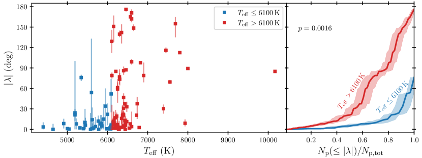
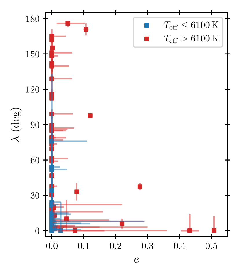
Winn et al. (2010) discovered that hot Jupiters orbiting cool stars have orbit normals that better align with stellar spin axes than hot Jupiters orbiting hot stars (see also e.g. Schlaufman, 2010; Albrecht et al., 2012; Winn et al., 2017; Muñoz & Perets, 2018; Albrecht et al., 2021; Hamer & Schlaufman, 2022; Siegel et al., 2023). Figure 1 displays this correlation between stellar obliquity $\lambda$ and stellar effective temperature $T_{\rm eff}$. Figure 2 shows that $T_{\rm eff}$ seems to correlate also with orbital eccentricity $e$: cooler stars host more circular hot Jupiters.

High-eccentricity migration is one way to form hot Jupiters (e.g. Dawson & Johnson 2018). One imagines that giant planets are delivered from afar onto high-$e$, high-$\lambda$, low-periastron orbits by, e.g., planet-planet scatterings or Lidov-Kozai oscillations. Presumably this initial delivery unfolds similarly around cool and hot stars. Subsequent tidal interactions with the star shrink the orbit by damping $e$ and orbital semi-major axis $a$. To reproduce the observations, tidal damping of $e$ and $\lambda$ would have to be, for some reason, more effective around cool stars than hot stars. In this paper we attempt to identify this reason.

The dividing line used in Figs. 1 and 2 to distinguish cool from hot stars is a stellar effective temperature $T_{\rm eff}=6100$ K, a.k.a. the Kraft break below which stars have convective envelopes and radiative cores, and above which stars have radiative envelopes and convective cores. Damping of the equilibrium tide, and by extension obliquity and eccentricity, has been argued to be more effective in turbulent convective envelopes, potentially explaining the $\lambda$-$T_{\rm eff}$ trend (Winn et al., 2010; Albrecht et al., 2012). A problem with this idea is that convective eddy turnover times may be much too long compared to tidal forcing periods for turbulent viscosity to be significant (Goldreich & Nicholson, 1977; Vidal & Barker, 2020). Even if convective dissipation (or the dissipation associated with the interaction between tidal flows and convection according to Terquem 2021; but see Barker & Astoul 2021) were somehow more effective, another problem with the equilibrium tide is that it results in wholesale semimajor axis decay. By the time the obliquity damps from equilibrium tidal dissipation, the star engulfs the planet (see also Barker & Ogilvie, 2009; Dawson, 2014).

Lai (2012) argued that dissipation of tidally excited inertial waves in convective zones could damp cool star obliquities while avoiding engulfment. One shortcoming of inertial wave dissipation is that it cannot take retrograde obliquities (which are observed for high-mass stars) and evolve them into prograde alignment (e.g. Rogers & Lin, 2013; Valsecchi & Rasio, 2014; Xue et al., 2014; Li & Winn, 2016; Anderson et al., 2021; Spalding & Winn, 2022). Another difficulty is that inertial wave dissipation scales with the host star’s spin rate, which may be too slow on the main sequence to damp obliquities (e.g. Lin & Ogilvie, 2017; Damiani & Mathis, 2018; Spalding & Winn, 2022). Dissipation rates are greater on the pre-main sequence, but observations indicate high-$\lambda$ systems form late (Hamer & Schlaufman, 2022), consistent with late-time dynamical instability in a high-$e$ migration scenario. Even if hot Jupiters formed early, high-mass stars have thick convective envelopes on the pre-main sequence, and inertial wave dissipation would predict their obliquities to be small, contrary to observation.

In this work we consider how $e$ and the (true 3D) obliquity $\psi$ evolve when the planet is resonantly locked with a stellar oscillation mode. The modes of interest are gravity modes (g modes), which exist in radiative (stably stratified) zones, not convective ones, and therefore behave differently between stars below and above the Kraft break. Gravity modes in the extensive radiative zones of stars have a dense frequency spectrum, and one can readily find a mode whose frequency matches (to within a low-integer factor) the planet’s orbital frequency. In resonance lock (Witte & Savonije, 1999, 2001; Savonije, 2008), the frequency match is preserved as a star evolves and its internal structure changes. Typically g-mode frequencies increase from increasing stratification due to hydrogen burning, and the planet’s orbital frequency follows suit — the planet migrates inward (Ma & Fuller, 2021). Resonance locks and stellar evolution can change not only orbital semi-major axis $a$, but also eccentricity $e$ (e.g. Savonije 2008; Fuller 2017; Zanazzi & Wu 2021). We show for the first time here that obliquity $\psi$ also evolves in resonance lock.

A full derivation of the equations governing $a$, $e$, and $\psi$ is given in appendix A; a condensed version sketching our physical picture and listing the main results is provided in section 2. How g-mode frequencies evolve differently between cool and hot stars is explored with MESA stellar evolution calculations in section 3. Results for the time evolution of $a$, $e$, and $\psi$ for proto-hot Jupiters in resonance lock are presented in section 4. Section 5 compares our theory with observations and offers some extensions, and section 6 concludes. In appendix B we consider the physics of g-mode energy dissipation to estimate the largest orbital distance out to which our theory applies.

2 Resonance Locking Model

Figure 3: Coordinate system used to analyze the coupling between stellar spin and planet orbit. The $z$-axis is chosen to always point in the direction of the stellar spin ${\bm{\hat{j}}}_{\star}$, and the $y$-axis is chosen to always point normal to ${\bm{\hat{j}}}_{\star}$ and ${\bm{\hat{j}}}_{\rm orb}$. The obliquity $\psi$ is the angle between ${\bm{\hat{j}}}_{\star}$ and ${\bm{\hat{j}}}_{\rm orb}$. In this paper we consider only the components of the tidal torque ${\bm{T}}$ which act to change $\psi$, i.e. only the $x$ and $z$-components.

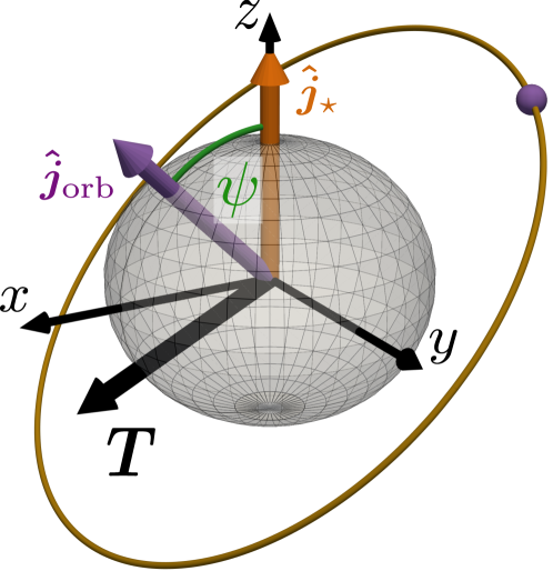
We begin with a general set of equations relating the angular momentum of the planet’s orbit with the angular momentum of the stellar spin. The star has mass $M_{\star}$, radius $R_{\star}$, spin frequency $\Omega_{\star}$, moment of inertia $I_{\star}=\kappa_{\star}M_{\star}R_{\star}^{2}$, and spin angular momentum ${\bm{J}}_{\star}=I_{\star}\Omega_{\star}{\bm{\hat{j}}}_{\star}$ with ${\bm{\hat{j}}}_{\star}$ the unit vector parallel to the stellar spin axis. The star is orbited by a planet of mass $M_{\rm p}\ll M_{\star}$, having orbital semi-major axis $a$, eccentricity $e$, mean-motion $\Omega=\sqrt{GM_{\star}/a^{3}}$, orbital energy $E_{\rm orb}=-GM_{\star}M_{\rm p}/(2a)$, and orbital angular momentum ${\bm{J}}_{\rm orb}=-(2\sqrt{1-e^{2}}E_{\rm orb}/\Omega){\bm{\hat{j}}}_{\rm orb}$, where $G$ is the gravitational constant and ${\bm{\hat{j}}}_{\rm orb}$ is the unit orbit normal. The stellar obliquity $\psi$ is the angle between ${\bm{J}}_{\star}$ and ${\bm{J}}_{\rm orb}$ ($\cos\psi={\bm{\hat{j}}}_{\rm orb}{\bm{\cdot}}{\bm{\hat{j}}}_{\star}$). We work in a Cartesian coordinate system such that ${\bm{\hat{j}}}_{\star}$ always lies in the $z$-direction, and ${\bm{\hat{j}}}_{\rm orb}$ always lies in the $x$-$z$ plane (i.e. ${\bm{\hat{j}}}_{\star}{\bm{\times}}{\bm{\hat{j}}}_{\rm orb}$ defines the $y$-direction). Energy is extracted from the orbit (from tidal dissipation) at a rate $\dot{E}_{\rm orb}<0$. Angular momentum is exchanged (by tides) between planet and star at rate ${\bm{T}}=-\dot{\bm{J}}_{\rm orb}=+\dot{\bm{J}}_{\star}$; we restrict consideration to the torque’s $x$ and $z$-components, ${\bm{T}}=T_{x}{\bm{\hat{e}}}_{x}+T_{z}{\bm{\hat{e}}}_{z}$, since $T_{y}$ just causes ${\bm{\hat{j}}}_{\rm orb}$ to precess about ${\bm{\hat{j}}}_{\star}$ without changing $\psi$. We thus have (Lai, 2012):

$$\frac{1}{a}\frac{{\rm d}a}{{\rm d}t}=-\frac{\dot{E}_{\rm orb}}{E_{\rm orb}},$$ (1)

$$\frac{{\rm d}J_{\star}}{{\rm d}t}=T_{z},$$ (2)

$$\frac{{\rm d}J_{\rm orb}}{{\rm d}t}=-T_{x}\sin\psi-T_{z}\cos\psi,$$ (3)

$$\frac{{\rm d}\psi}{{\rm d}t}=-\frac{T_{x}}{J_{\star}}-\frac{T_{x}}{J_{\rm orb}}\cos\psi+\frac{T_{z}}{J_{\rm orb}}\sin\psi.$$ (4)

See Figure 3 for an illustration of the coordinate system in which we are working.

Figure 4: An axisymmetric $m=0$ oscillation on the host star (top left) can be excited by the dominant $k=m_{\rm orb}=2$ component of the planet’s tidal potential (top right) when $\psi>0$ (bottom right showing that the radial tidal force integrated over the stellar equator is net outward). When $\psi=0$, tidal forces cancel over stellar azimuth and the $m=0$ mode cannot be excited (bottom left).

Figure 5: How a planet can tidally torque the host star into spin-orbit alignment, by way of an axisymmetric $m=0$ g-mode oscillation forced by the planet’s $k=m_{\rm orb}=2$ potential. The star stretches and compresses along its spin axis ($z$-axis) twice for every orbit of the planet. The solid purple sphere marks the planet’s location which is displaced ahead of the star’s tidal bulge due to tidal friction, while the see-through purple sphere displays the planet’s location in the absence of tidal friction. The top row shows different views of the same instant in time, when the star is maximally elongated but the planet is ahead at positive $y$. The bottom row shows a different time, when the star is maximally compressed and similarly lagged in phase relative to the planet. The tidal bulge at position vector ${\bm{r}}$ feels a force from the planet ${\bm{F}}$ and by extension a torque ${\bm{T}}={\bm{r}}\times{\bm{F}}$ that is positive in the $x$-direction no matter the orbital phase (middle column). The torque $T_{x}>0$ acts to bring the stellar spin direction (${\bm{\hat{j}}}_{\star}$) toward the $x$-axis, closer to the orbital angular momentum direction (${\bm{\hat{j}}}_{\rm orb}$). Once spin and orbit are aligned, the torque vanishes (Fig. 4, bottom left panel). Because the oscillation is symmetric about the $z$-axis (right column), there is no torque in the $z$-direction.

Our theory is that $\dot{E}_{\rm orb}$ and ${\bm{T}}$ are driven predominantly by a particular oscillation mode in the star, resonantly excited by the planet. In resonance, an integer multiple $k$ of the planet’s orbital frequency matches the stellar oscillation frequency:

$$k\Omega=\sigma_{\alpha}=\omega_{\alpha}+m\Omega_{\star}$$ (5)

where $\sigma_{\alpha}$ is the mode oscillation frequency in the inertial frame, $\omega_{\alpha}$ is the oscillation frequency in the frame rotating with the star, and $m$ is the mode’s azimuthal number. For most of this paper, we restrict attention for simplicity to “zonal” $m=0$ axisymmetric modes (Zanazzi & Wu, 2021).

In resonance lock, oscillation and orbit track one another; the mode frequency evolves on the same timescale as the orbit evolves:

$$t_{\rm ev}^{-1}\equiv\frac{\dot{\sigma}_{\alpha}}{\sigma_{\alpha}}=\eta_{\alpha}\frac{\dot{E}_{\rm orb}}{E_{\rm orb}}$$ (6)

where $\eta_{\alpha}=3/2$ for $m=0$ (see appendix A and Fuller 2017 for the case $m\neq 0$). In this paper, we assume the planet locks onto a stellar gravity mode (g mode), and compute how $\dot{\sigma}_{\alpha}/\sigma_{\alpha}$ evolves on the stellar main sequence (section 3).

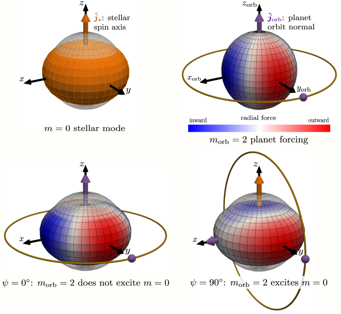
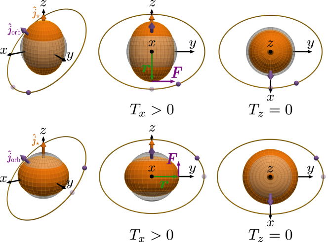
In the inertial frame co-planar with the orbit, each term in the planet’s tidal forcing potential varies as

$$\exp\left(-{\rm i}k\Omega t+{\rm i}m_{\rm orb}\varphi_{\rm orb}\right)$$ (7)

where $\varphi_{\rm orb}$ is the azimuthal coordinate measured in the orbital plane; note that $m_{\rm orb}$ differs from the stellar mode azimuthal number $m$ defined earlier. The dominant term in the forcing potential has $k=m_{\rm orb}=2$. Figure 4 illustrates how $k=m_{\rm orb}=2$ tidal forcing can excite an $m=0$ mode in the star for $\psi\neq 0$ (bottom right panel), and conversely how $\psi=0$ represents a fixed point where an $m=0$ mode is not excited (bottom left). Figure 5 illustrates how this $m=0$ mode causes the obliquity to damp — the planet exerts a torque on the tidally lagged stellar bulge that always acts to bring the stellar spin vector into closer alignment with the orbit normal, at all orbital phases of the planet. Only when spin and orbit align does the torque vanish. Thus, the $\psi=0$ fixed point is a stable attractor — the obliquity under many initial conditions damps to zero.

We evaluate equations (1)-(4) for the case when planet and star are in resonance lock for $\{k,\ell,m\}=\{2,2,0\}$, where $\ell$ is the angular degree of the spherical harmonic representing the stellar oscillation mode (for context, most other studies of tidally forced oscillations focus on $\ell=2$, $m=2$). The full derivation is relegated to appendix A; the results are:

$$\frac{1}{a}\frac{{\rm d}a}{{\rm d}t}=-\frac{1}{\eta_{\alpha}t_{\rm ev}}$$ (8)

$$\frac{{\rm d}J_{\star}}{{\rm d}t}=\ 0$$ (9)

$$\frac{{\rm d}e}{{\rm d}t}=-\frac{1-e^{2}}{2e}\bigg{(}1-\frac{\sin\psi}{2\sqrt{1-e^{2}}}\tau\bigg{)}\frac{1}{\eta_{\alpha}t_{\rm ev}}$$ (10)

$$\frac{{\rm d}\psi}{{\rm d}t}=-\frac{1}{4\sqrt{1-e^{2}}}\left(\frac{J_{\rm orb}}{J_{\star}}+\cos\psi\right)\tau\frac{1}{\eta_{\alpha}t_{\rm ev}}.$$ (11)

Note that $J_{\star}$ does not change ($T_{z}=0$; Fig. 5, right column) because we are considering only axisymmetric stellar modes (see section 5.6 and appendix A for a discussion of non-axisymmetric modes). The dimensionless torque $\tau=2\Omega T_{x}/\dot{E}$ is given by equation (A43), and depends on $e$ through Hansen coefficients $X^{k}_{\ell,m_{\rm orb}}$ and $\psi$ by a sum over Wigner-$d$ matrix coefficients (eq. A9). When $\psi\ll 1$ and $e\gg\psi$,

$$\tau\simeq\frac{9}{8}\left(\frac{X^{2}_{2,2}}{X^{2}_{2,0}}\right)^{2}\psi^{3}$$ (12)

which vanishes as $\psi\to 0$. Equations (8) and (10) then imply $a(1-e^{2})\simeq\text{constant}$, i.e. the orbit circularizes along a constant angular momentum track (Zanazzi & Wu, 2021). In the opposite case when $e\ll 1$ and $\psi\gg e$,

$$\tau\simeq\frac{2}{\sin\psi}$$ (13)

and the obliquity changes at a rate

$$\frac{{\rm d}\psi}{{\rm d}t}\simeq-\left(\frac{J_{\rm orb}}{J_{\star}}+\cos\psi\right)\frac{1}{2\sin\psi}\frac{1}{\eta_{\alpha}t_{\rm ev}}.$$ (14)

Obliquities damp if they are not too retrograde ($\cos\psi>-J_{\rm orb}/J_{\star}$). For hot Jupiters orbiting main-sequence stars with masses $\lesssim 1\,{\rm M}_{\odot}$, obliquities should always damp because for such stars $J_{\rm orb}/J_{\star}>1$, in part because they are centrally concentrated and have small $\kappa_{\star}$.

3 Gravity Mode Evolution Between Low-Mass and High-Mass Stars

Figure 6: Rate of Brunt-Väisälä frequency evolution (top panel, eq. 16) and accumulated frequency change (middle panel, eq. 18) vs. main-sequence age, for stars of different masses as indicated. Although high-mass stars (red curves) increase their frequencies dramatically quickly toward the end of their hydrogen-burning lives (as their cores switch from being unstably to stably stratified), the speed-up phase is short-lived and consequently unlikely to be observed. Sampled over the entirety of their main-sequence lives, $\Delta N/\langle N_{0}\rangle$ is likely to be higher for low-mass stars, whose cores remain stably stratified throughout, than for high-mass stars (bottom panel showing median and $\pm 1\sigma$ intervals).

In the low-frequency limit, g-mode frequencies in the host star’s rotating frame are given by

$$\omega_{\alpha}\simeq\frac{\sqrt{\ell(\ell+1)}}{\pi n}\langle N\rangle,$$ (15)

where $n\gg 1$ is the number of radial nodes, and the radial average of the Brunt-Väisälä frequency is given by

$$\langle N\rangle=\int_{\rm rad}\frac{N}{r}{\rm d}r,$$ (16)

with the integral being taken over the stably stratified radiative zone ($N^{2}>0$). As in Zanazzi & Wu (2021), we focus on zonal modes (azimuthal number $m=0$), so $\omega=\sigma$, and $t_{\rm ev}$ is given by

$$t_{\rm ev}^{-1}=\frac{\langle\dot{N}\rangle}{\langle N\rangle}$$ (17)

ignoring Coriolis forces.

We define a fractional frequency change

$$\frac{\Delta N(t)}{\langle N_{0}\rangle}\equiv\frac{\langle N(t)\rangle-\langle N_{0}\rangle}{\langle N_{0}\rangle}$$ (18)

and use the stellar evolution code MESA (release r23.05.1) to compute $\langle N(t)\rangle$ from $t_{0}\equiv 1\,{\rm Gyr}$ to $t_{\rm max}=\min(t_{\rm MS},12\,{\rm Gyr})$, with the end of the main-sequence lifetime $t_{\rm MS}$ defined by when the star’s core begins helium burning (the subscript 0 denotes evaluation at time $t_{0}$). The MESA inlists we use are identical to those in Fuller (2017). How our results depend on $t_{0}$ and $t_{\rm max}$ is discussed in section 5.3.

Figure 7: Orbital evolution of hot Jupiters in resonance lock with a stellar gravity mode ($\{k,l,m\}=\{2,2,0\}$), integrated from $t_{0}=1$ Gyr through the stellar main-sequence lifetime or $t=12$ Gyr, whichever comes first. Here planet orbits are assumed circular for all time. Obliquities damp more readily for cool stars (blue curves) than hot stars (red curves). For hot stars with $\psi_{0}=145^{\circ}$, obliquities actually increase slightly, a consequence of their having $J_{\rm orb}/J_{\star}<1$ (unlike for cool stars).

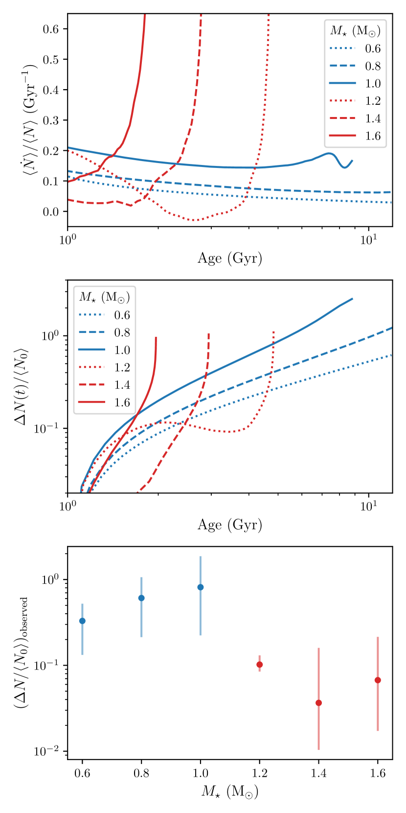
Over the star’s main sequence lifetime, in response to the loss of gas pressure from the conversion of hydrogen into helium and the increase in mean molecular weight, the core contracts and becomes more dense and stratified. Thus $\langle N\rangle$ tends to increase, the more so when the region of stable stratification extends down to the star’s core, as it typically does for cool but not for hot stars. Figure 6 illustrates how the evolution of the star-averaged Brunt-Väisälä frequency differs between cool low-mass stars (blue curves) and hot high-mass stars (red curves). The sign of the difference can be subtle and varies with context. The top panel of Fig. 6 shows that for high-mass stars at the end of their main-sequence lifetimes, the mode evolution rate $\langle\dot{N}\rangle/\langle N\rangle$ actually exceeds that for low-mass stars — see how the red curves ultimately skyrocket above the blue curves. The last-minute speed up of mode evolution in high-mass stars, which occurs as they ascend the sub-giant branch and their cores switch from being convective to radiative, is so great that even though low-mass stars live longer than high-mass stars, the total change $\Delta N$ accumulated over main-sequence lifetimes is comparable between low-mass and high-mass stars (middle panel of Fig. 6). Nevertheless, because the mode frequency speed-up for high-mass stars occurs over a small fraction of the high-mass main-sequence lifetime, the time-averaged value for $\Delta N$ is actually lower for high-mass as compared to low-mass stars (bottom panel of Fig. 6). The upshot is that given a low-mass main-sequence star and a high-mass main sequence star drawn randomly from the field, the low-mass star is more likely to have experienced a larger fractional change in its g-mode frequency. The expected change is on the order of unity for low-mass stars, and $\lesssim 10\%$ for high-mass stars. This difference underpins our theory that stellar obliquities have evolved more for low-mass than high-mass stars.

Figure 8: Same as Fig. 7 except for initial eccentricities $e_{0}=0.3$. For such initial conditions, orbits circularize rapidly around both cool and hot stars, faster than the obliquity damps. The obliquity evolution is largely the same as for strictly circular orbits (compare with Fig. 7).

Figure 9: Same as Figs. 7 and 8 except for initial conditions $\{e_{0},a_{0}\}=\{0.6,0.07\,{\rm AU}\}$. At these larger eccentricities, damping of $\psi$, $e$, and $a$ takes longer, but the equilibrium fixed point of $\psi,e=0$ can still be reached within main-sequence lifetimes for cool stars whose obliquities are not too high. Hot star obliquities remain near their initial values regardless.

4 Results for Obliquity and Orbit Evolution

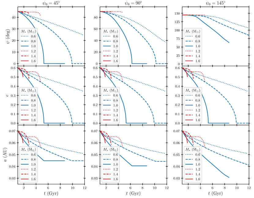
We integrate equations (8)-(11) for a planet of mass $M_{\rm p}=1\,{\rm M}_{\rm J}$ in resonant lock with a stellar gravity mode. We start all calculations at time $t_{0}=1\,{\rm Gyr}$, and evolve $\psi$, $e$, and $a$ to $t_{\rm max}=\min(t_{\rm MS},12\,{\rm Gyr})$, where $t_{\rm MS}$ is the time when the stellar core begins burning helium. Note that if and when both $\psi,e=0$, resonance lock with our assumed $\{k,\ell,m\}=\{2,2,0\}$ mode cannot be maintained (e.g. bottom left panel of Fig. 4), and $a$, $e$, and $\psi$ cease to change. In section 5.2 and appendix B we discuss more generally how resonance locks may actually break. Initial conditions vary over $a_{0}=\{0.035,0.07\}$ AU, $e_{0}=\{0,0.3,0.6\}$, and $\psi_{0}=\{45^{\circ},90^{\circ},145^{\circ}\}$ (variables subscripted 0 are evaluated at time $t_{0}$). We integrate our equations using the Python routine solve_ivp from scipy, setting $\texttt{rtol}=10^{-6}$ and $\texttt{atol}=10^{-11}$, and evaluating $t_{\rm ev}^{-1}$ by linear interpolation (using numpy interp) of the data in the top panel of Fig. 6.

Stellar input parameters to equations (8)-(11) are computed with MESA for stars of mass $M_{\star}=\{0.6,0.8,1.0,1.2,1.4,1.6\}\,{\rm M}_{\odot}$; these parameters include $t_{\rm ev}$ (equations 16-17), $R_{\star}(t)$, and

$$\kappa_{\star}(t)=\frac{4\pi}{M_{\star}R_{\star}^{2}}\int_{0}^{R_{\star}}\rho r^{4}{\rm d}r$$ (19)

where $\rho$ is the stellar mass density. We set the initial spin rate $\Omega_{\star 0}=2\pi/(20\ {\rm d})$ for stars below the Kraft break (“cool” or “low-mass”, $M_{\star}<1.2\,{\rm M}_{\odot}$), and $\Omega_{\star 0}=2\pi/(5\ {\rm d})$ for stars above (“hot” or “high-mass”, $M_{\star}\geq 1.2\,{\rm M}_{\odot}$). These choices set $J_{\star}=\kappa_{\star}M_{\star}R_{\star}^{2}\Omega_{\star}=\text{constant}$ (eq. 9), determining $\Omega_{\star}(t)$ (which hardly changes in this simplified model). For reference, as mass increases from 0.6 to 1.6 ${\rm M}_{\odot}$ for our model stars, $\kappa_{\star 0}$ decreases from $\sim$0.22 to $\sim$0.05, $R_{\star 0}/a_{0}$ increases from $\sim$0.07 to $\sim$0.24 at $a_{0}=0.035$ AU, $\Omega_{\star 0}/\Omega_{0}$ increases from $\sim$$0.13$ to $\sim$$0.4$, and $J_{\rm orb,0}/J_{\star 0}$ decreases from $\sim$$8.4$ to $\sim$$0.5$. For our low-mass stars, $J_{\rm orb}/J_{\star}>1$ throughout the system evolution, a condition important for damping obliquity (see equation 14 and related discussion).

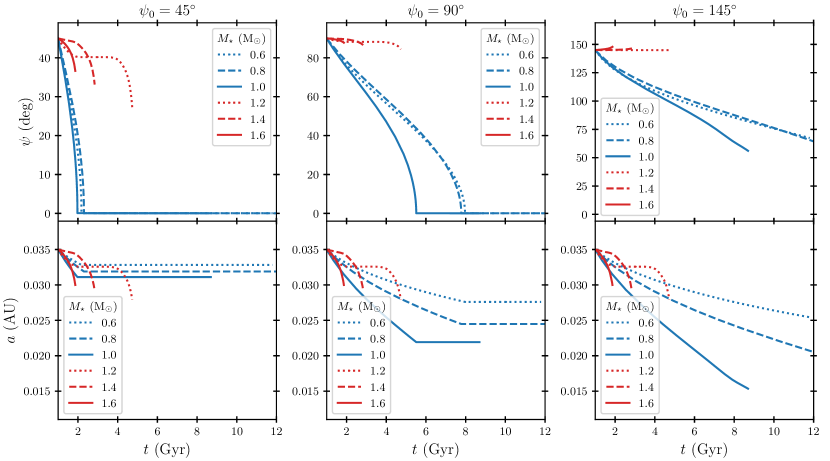
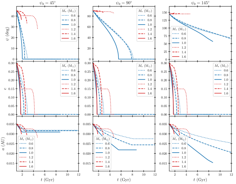
Figures 7, 8, and 9 present results for initial conditions $e_{0}=0$, 0.3, and 0.6, respectively. In all cases, obliquities $\psi$ damp more for low-mass stars than high-mass stars. For low-mass stars, obliquities can start as high as $90^{\circ}$ and drop to zero within main-sequence lifetimes. Once the obliquity vanishes, the planet can no longer drive the $m=0$ mode that we are modeling; dissipation ceases and the planet stops migrating inward. For high-mass stars, obliquities hardly budge from their initial values. None of our planets is engulfed by its host star.

A starting eccentricity of 0.3 damps to zero within main-sequence lifetimes for both low-mass and high-mass stars (Fig. 8), faster than the obliquity damps. At $e_{0}=0.6$, only the 1 and 0.8 ${\rm M}_{\odot}$ models circularize within 12 Gyr (Fig. 9). Large eccentricities are seen to prolong obliquity damping times (compare Figs. 8 and 9).

Figure 10: A population synthesis based on resonance locking (open symbols) compared against observations (filled symbols). Data for projected obliquities $\lambda$ (top) and obliquities $\psi$ (bottom) are taken from Albrecht et al. (2022), Rice et al. (2022a, b), Siegel et al. (2023), Espinoza-Retamal et al. (2023), Sedaghati et al. (2023), and Hu et al. (2024), for hot Jupiters ($M_{\rm p}\geq 0.3\,{\rm M}_{\rm J}$, $a/R_{\star}\leq 10$) above and below the Kraft break ($T_{\rm eff}\leq 6100\,{\rm K}$ in blue, $T_{\rm eff}>6100\,{\rm K}$ in red). In the model, obliquities are initially random (uniformly distributed in $\cos\psi_{0}$ between $-1$ and $1$), and subsequently damp by resonance locking over Gyr timescales. Damping is seen to be negligible for most hot stars (excepting those with $\psi_{0}\lesssim 25^{\circ}$ which damp to zero), but significant for cool stars. Although roughly reproducing the break seen in the observations, the model fails to damp sufficiently cool star obliquities that start strongly retrograde; these evolve into the cloud of blue open symbols with obliquities between $25^{\circ}$ and $90^{\circ}$ sitting above the observations.

5 Discussion

We have shown that hot Jupiters locked in resonance with stellar g-modes can torque the stars into spin-orbit alignment and have their orbits circularized. The damping of obliquity and eccentricity is stronger for lower-mass stars because their g-mode frequencies evolve more on the main sequence. In the following subsections we delve deeper into the theory, and confront observations.

5.1 Obliquity and Stellar Effective Temperature:
Theory vs. Observation

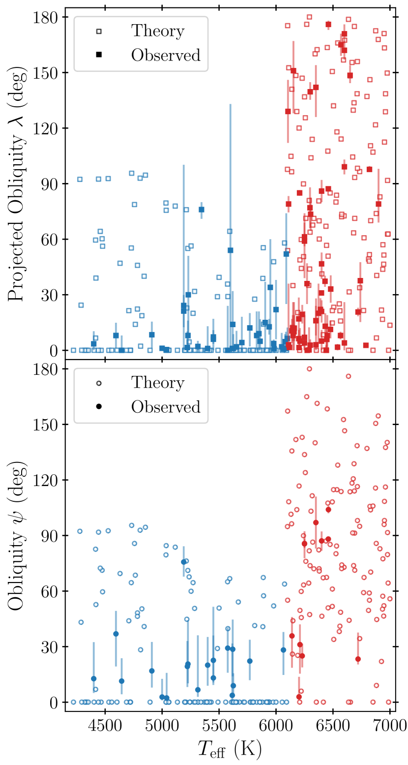
We construct a simple population synthesis to compare against observations. Host stellar masses $M_{\star}$ are sampled uniformly from the set $\{0.6,0.8,1.0,1.2,1.4,1.6\}\ {\rm M}_{\odot}$. Around each star we consider a planet of mass $M_{\rm p}=1\,{\rm M}_{\rm J}$, initial semimajor axis $a_{0}=8R_{\star 0}$, eccentricity $e_{0}=0$, and obliquity $\psi_{0}$ drawn randomly from a uniform distribution in $\cos\psi_{0}$ between $-1$ and 1 (for observational support of the latter distribution, see Siegel et al. 2023 and Dong & Foreman-Mackey 2023). Our equations of motion are then integrated from $t_{0}=1\ {\rm Gyr}$ to $t_{\rm max}$ (either 12 Gyr or the main-sequence lifetime, whichever comes first), and the final values for $\psi$ extracted for comparison with observations. Since the observations typically trace stellar effective temperature $T_{\rm eff}$ instead of stellar mass, we map our set of 6 $M_{\star}$ values to the uniform intervals $\{[4200,5000]$, $[5000,5600]$, $[5600,6100]$, $[6100,6400]$, $[6400,6700]$, $[6700,7000]\}\ {\rm K}$, drawing randomly from each interval. Furthermore, since most measured obliquities are projected obliquities $\lambda$, we perform mock observations to convert obliquities into projected obliquities using

$$\tan\lambda\simeq\tan\psi\sin\phi_{\rm obs},$$ (20)

drawing $\phi_{\rm obs}$ randomly from a uniform distribution between 0 and $2\pi$ (e.g. Fabrycky & Winn, 2009).

Figure 10 compares our modeled projected obliquities $\lambda$ with those observed (top panel; observations from Rice et al. 2022a). For completeness, we also show our modeled obliquities $\psi$ against the few true (deprojected) obliquities that are available (bottom panel; data from Albrecht et al. 2022; Siegel et al. 2023). Broadly speaking, our model reproduces the dichotomy between hot oblique stars above the Kraft break, and cool aligned stars below. Obliquities of hot stars hardly change in our theory from their assumed initially isotropic distribution. Obliquities of cool stars are damped, all the way to zero if they start from $\psi_{0}\lesssim 90^{\circ}$. Our model hot Jupiters have final semi-major axes $a\gtrsim 2.7R_{\star}$ and thus avoid tidal disruption (e.g. Guillochon et al., 2011) and stellar engulfment (e.g. Barker & Ogilvie, 2009; Winn et al., 2010; Dawson, 2014).

Fig. 10 also shows that our theory may over-predict the obliquities of the coolest (K-type) stars. If the initial obliquities are retrograde ($\psi_{0}\gtrsim 90^{\circ}$ for 0.6 ${\rm M}_{\odot}$ stars, and $\psi_{0}\gtrsim 120^{\circ}$ for 1.0 ${\rm M}_{\odot}$ stars), they evolve to become prograde but do not reach zero — see the cloud of open symbols from our model at $T_{\rm eff}\lesssim 5100\ {\rm K}$, and contrast with the filled symbols at low obliquity from observations. Other shortcomings of our population synthesis include our neglect of initially non-zero eccentricities (which would lengthen obliquity damping times and worsen the discrepancy between theory and observation for cool stars) and our neglect of a distribution of initial semi-major axes.

5.2 Breaking Resonance Locks: $\psi_{\rm break}$ vs. $a$

Figure 11: Charting the limits of resonance locking. Computed curves are for an axisymmetric ($m=0$) g-mode of a $1\,{\rm M}_{\odot}$, 4-Gyr-old main-sequence star (see appendix B). The green bar ($\psi_{\rm break}^{\rm lin}$) marks an uncertain transition region dividing the space where resonance locking can operate (to the left) from where it cannot (to the right), computed under the assumption that tidal disturbances are linear and damp by radiative diffusion. In purple are plotted the analogous boundaries for $\psi_{\rm break}^{\rm nl}$, computed assuming tidal disturbances are limited in amplitude by nonlinear mode-mode couplings. The nonlinear model expands the regime where resonance locking is possible, out to $a/R_{\star}\approx 8$. Overlaid for context are observed projected obliquities $\lambda$ (Albrecht et al., 2022; Rice et al., 2022a, b; Siegel et al., 2023; Espinoza-Retamal et al., 2023; Sedaghati et al., 2023; Hu et al., 2024). See section 5.2 for how we might interpret these data.

As stellar obliquity decreases, tidal forcing of zonal g-modes weakens (see, e.g., the bottom left panel of Fig. 4). There are obliquity boundaries $\psi_{\rm break}$ beyond which resonant locks fail. These boundaries depend on how tidal disturbances damp.

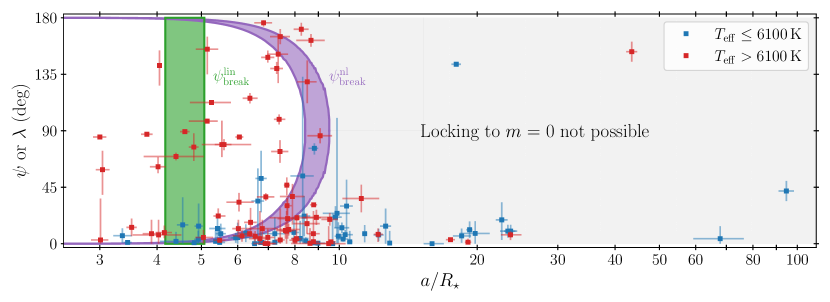
How tidally-driven modes damp is uncertain. We attempt two calculations, one using a “linear” damping rate for how waves lose energy to radiative diffusion when wave amplitudes are small, and another based on “non-linear” interactions that siphon energy away from tidally-driven modes to other stellar modes. Details are contained in appendix B. Results for $\psi_{\rm break}$, computed for a 4-Gyr-old solar-mass star, are presented in Figure 11. According to the linear theory (green bar), resonance locking can fully damp obliquities for $a/R_{\star}<4$, but not for $a/R_{\star}>5$. Nonlinear damping can extend the reach of resonance locks out to $a/R_{\star}\approx 7$-$8$ (purple curves). We reiterate that these results for $\psi_{\rm break}$ are highly uncertain and specific to a $1\,{\rm M}_{\odot}$ star.

Interestingly, as seen in Fig. 11, most measured projected obliquities $\lambda$ of cool stars appear small at semi-major axes as far out as $a/R_{\star}\sim 100$ (see also Morgan et al., 2024). Our interpretation is that for stars beyond the resonance locking limit ($a/R_{\star}>8$ according to the nonlinear damping theory), small obliquities are primordial: Jupiter-mass planets accreted from disks aligned with stellar equatorial planes. This interpretation may also apply to the mostly small obliquities observed for hot stars with exo-Jupiters at large $a/R_{\star}\sim 20$ (with large-obliquity outliers tending to be in stellar binaries; Rice et al. 2022b). By contrast, at $a/R_{\star}<8$, hot stars are observed to have large obliquities, presumably the result of whatever process created hot Jupiters (e.g. planet-planet scatterings / high-eccentricity migration). Hot star obliquities hardly damp from resonance locking because the g-mode frequencies of hot stars, which lack radiative cores, change by $\lesssim 10\%$ over most of their main sequence lives (sections 3 and 4). If hot Jupiters form around cool stars the same way they do around hot stars, they would be similarly initially misaligned. We have shown that cool star misalignments can be subsequently erased in resonance lock, as their radiative cores become more strongly stratified and g-mode frequencies increase.

5.3 Stellar Ages and Resonance Locking Duration

Our calculations of resonance locking start at $t_{0}=1\ {\rm Gyr}$, when our higher-mass stars have only $\sim$1–3 Gyr left before they ascend the subgiant branch. We have checked that the calculations shown Figs. 7-9 are robust to changes in $t_{0}$ down to 0.1 Gyr. Starting times of 0.1–1 Gyr appear consistent with high-eccentricity migration, which takes of order such times to form hot Jupiters on initially misaligned orbits (e.g. Dawson & Johnson, 2018; Wu, 2018; Vick et al., 2019). Similarly long gestation times are indicated by the observation that misaligned hot Jupiter hosts have higher Galactic velocity dispersions and are therefore older than aligned hosts (Hamer & Schlaufman, 2022).

Late formation of misaligned hot Jupiters bypasses resonance locks that occur during the pre-main sequence (Zanazzi & Wu, 2021). Pre-main sequence locks would predict little difference in tidal evolution with stellar mass, as young stars have similar internal structures (mostly convective) irrespective of mass (e.g. Henyey et al., 1955).

Once high-mass stars depart the main sequence, their obliquities should damp as their Brunt-Väisälä frequencies climb rapidly (Fig. 6 middle panel). Our model predicts that evolved stars hosting hot Jupiters should have small obliquities.

5.4 Obliquity vs. Eccentricity

We have found that resonance locking damps eccentricity, more so for lower mass stars, and that eccentricities damp to zero faster than obliquities do (Figs. 8 and 9). These theoretical expectations appear consistent with the observational data in Figure 2; there are no high-$e$, low-$\lambda$ hot Jupiter systems around cool stars.

5.5 Obliquity vs. Planet Mass

We have focused in this work on Jupiter-mass planets as these have some of the most reliable obliquity measurements. Lower planet masses decrease obliquity damping rates (approximately linearly through the term $J_{\rm orb}\propto M_{\rm p}$ in equation 11) and increase $\psi_{\rm min}$ (section 5.2). Accordingly, we would not expect stars hosting hot sub-Neptunes to exhibit the same obliquity trends shown by stars hosting hot Jupiters. Observations appear to support this expectation (e.g. Hébrard et al., 2011; Albrecht et al., 2022), although Louden et al. (2021) found from rotational broadening measurements that cool host stars of sub-Neptunes may be more aligned than hot host stars.

Conversely, more massive planets should damp stellar obliquities faster. Hébrard et al. (2011) and Albrecht et al. (2022) have noted that “moderately” hot stars ($6250\,{\rm K}\lesssim T_{\rm eff}\lesssim 7000\,{\rm K}$; $1.3\,{\rm M}_{\odot}\lesssim M_{\star}\lesssim 1.6\,{\rm M}_{\odot}$), when orbited by brown dwarfs ($M_{\rm p}\gtrsim 10\,{\rm M}_{\rm J}$), display small obliquities (see e.g. Albrecht et al. 2022 Figure 9, middle panel).

5.6 Non-Axisymmetric Modes

We have focussed in this work on the $m=0$ axisymmetric stellar g-mode and how it damps obliquity. In appendix A we show that obliquity damps for a g-mode with all $|m|\leq\ell$, when forced into resonance lock by the $\{k,\ell\}=\{2,2\}$ component of the tidal potential, for a circular planet with $J_{\rm orb}>J_{\star}$. The obliquity damps as (eq. A42)

$$\frac{{\rm d}\psi}{{\rm d}t}=-\left[\tau_{m}\left(\frac{J_{\rm orb}}{J_{\star}}+\cos\psi\right)-m\sin\psi\right]\frac{1}{4\eta_{\alpha}t_{\rm ev}}.$$ (21)

The parameter $\eta_{\alpha}$ remains close to $3/2$ for typical hot Jupiter systems (Ma & Fuller, 2021). For $m=0$, the torque coefficient $\tau_{0}=2/\sin\psi$, while for $m=\pm 1$ and $m=\pm 2$,

$$\tau_{\pm 1}=\frac{2\mp\cos\psi}{\sin\psi},\hskip 14.22636pt\tau_{\pm 2}=\frac{2\sin\psi}{1\pm\cos\psi}.$$ (22)

These torque coefficients are always positive, and for $J_{\rm orb}~{}>~{}J_{\star}$, they lead to the first term in (21) dominating the second term, giving ${\rm d}\psi/{\rm d}t<0$ for all $\psi$.

Calculating the detailed time history of $\psi$ for $m\neq 0$ is left for future work. Here we offer some comments and speculation. The likelihood of locking onto a mode of given $m$ should be proportional to the amplitude of the tidal potential $|U^{2}_{2m2}|$ (eq. A6). Whereas polar planets ($\psi\approx\pi/2$) are favored to lock onto zonal g-modes ($m=0$), prograde obliquities ($\psi<\pi/2$) will likely lock onto prograde modes ($m>0$), and retrograde obliquities ($\psi>\pi/2$) onto retrograde modes ($m<0$). Because prograde locks have weaker alignment torques ($\tau_{1},\tau_{2}<\tau_{0}$ when $\psi<\pi/2$) and spin up the host star ($\dot{J}_{\star}\propto m>0$, eq. A40), they will damp prograde obliquities more slowly than zonal locks. Ma & Fuller (2021) found that the spin-up of hot Jupiter hosts from sectoral ($m=2$) locks may help explain their rapid rotation rates (Penev et al., 2018). Relative to zonal locks, retrograde locks may damp initially retrograde obliquities more slowly, but once the obliquity swings to prograde, damping may be faster because alignment torques are stronger ($\tau_{-2},\tau_{-1}>\tau_{0}$ when $\psi<\pi/2$) and because retrograde locks spin down the star ($\dot{J}_{\star}<0$).

6 Summary

A planet can tidally force a stellar gravity mode (g mode), with consequences for the planet’s orbit and the star’s spin. Structural changes inside the star over the course of its evolution can change the companion’s orbit so as to maintain a commensurability between the orbital frequency and the g-mode oscillation frequency. Such resonance locking can alter orbital semi-major axes and eccentricities, and stellar rotation rates (e.g. Zanazzi & Wu, 2021; Ma & Fuller, 2021). The direction of the stellar spin axis relative to the planet’s orbit normal can also change in resonance lock, as we have established in this paper.

Stars that host hot Jupiters are known to have spin axes misaligned from their orbit normals. Large stellar obliquities are thought to be a relic of the gravitational scatterings and long-term dynamical perturbations that originally delivered hot Jupiters onto their close-in orbits (e.g. Dawson & Johnson, 2018). Primordial spin-orbit misalignments appear to have been preserved for host stars with effective temperatures $T_{\rm eff}\gtrsim 6100$ K, but may have damped away for cooler stars with near-circular planets (Winn et al., 2010; Rice et al., 2022a). We have shown how obliquity damping goes hand-in-hand with semi-major axis and eccentricity damping when star and planet are resonantly locked. While on the main sequence, cooler stars experience much more damping than hotter stars. The dependence on $T_{\rm eff}$ arises because stellar g-modes are sustained only in stably stratified radiative zones, and cool stars have radiative cores whose g-mode (Brunt-Väisälä) frequencies increase substantially from core hydrogen burning, thereby driving significant tidal evolution. Hotter stars lack such cores. Thus resonance locking can explain how cooler stars are aligned with hot Jupiters while hotter stars are not.

As a simplification, we assumed throughout most of our work that the planet locks to an axisymmetric (zonal) gravity mode. The obliquity damps whether the planet locks to an axisymmetric or non-axisymmetric gravity mode, but the efficiency of damping will vary with the azimuthal wavenumber $m$, possibly significantly. For $m=0$, we found that damping may not be strong enough to bring initial obliquities $\gtrsim 90^{\circ}$ for the coolest K-type stars down to $\lesssim 30^{\circ}$ as observed. More work also needs to be done on understanding how mode energies damp, to determine more accurately the orbital distances out to which resonance locking can work.

We thank Simon Albrecht, Linhao Ma, Diego Munoz, and Joshua Winn for discussions. Financial support was provided by a 51 Pegasi b Heising-Simons Fellowship awarded to JJZ. EC acknowledges support from a Simons Investigator award and NSF AST grant 2205500.

Appendix A Energy and Angular Momentum Transfer from an Inclined, Eccentric Planet to a Spinning Star

This appendix considers the general case of an eccentric planet inclined to the star’s equitorial plane, and calculates the energy and angular momentum exchange rate between the orbit of the planet, and a general stellar oscillation. We also calculate the orbital evolution which results from this angular momentum loss.

A.1 Tidal Potential

Figure 12: Plotting the magnitude of the Hansen coefficients (eq. A2), for the $\{k,\ell\}=\{2,2\}$ component of the tidal potential. The $|X^{2}_{2,2}|$ coefficient dip at $e\sim 0.7$ occurs because $X^{2}_{2,2}$ changes sign. The $|X^{2}_{2,2}|$ coefficient is larger than $|X^{2}_{2,0}|$ at smaller eccentricities, until $e\gtrsim 0.4-0.5$. We always have $|X^{2}_{2,-2}|\ll|X^{2}_{2,0}|$.

In a spherical coordinate system $(r,\theta_{\rm orb},\varphi_{\rm orb})$ centered on the star, with the $z_{\rm orb}$-axis parallel to the planet’s orbit normal and the $x_{\rm orb}$-axis pointing towards pericenter, the tidal potential is given by (e.g. Zanazzi & Wu, 2021)

$$U=-\frac{GM_{\rm p}}{a}\sum_{\ell=2}^{\infty}\sum_{m_{\rm orb}=-\ell}^{\ell}\left(\frac{r}{a}\right)^{\ell}W_{\ell m_{\rm orb}}\sum_{k=-\infty}^{\infty}X_{\ell m_{\rm orb}}^{k}(e){\rm e}^{-{\rm i}k\Omega t}Y_{\ell m_{\rm orb}}(\theta_{\rm orb},\varphi_{\rm orb}).$$ (A1)

Here, $k$ is the orbital harmonic, $\ell$ is the angular degree, $m_{\rm orb}$ is the azimuthal number of the tidal potential in a coordinate system centered on the planet’s orbital plane, $W_{\ell m}$ is given by equation (24) of Press & Teukolsky (1977), while

$$X_{\ell m}^{k}(e)=\frac{1}{\pi}\int_{0}^{\pi}{\rm d}E\frac{\cos[k(E-e\sin E)-mf]}{(1-e\cos E)^{\ell}},$$ (A2)

are Hansen coefficients, with $f$ the true anomaly. Notice the eccentricity $e$ and exponential ${\rm e}$ differ typographically. For $\ell=2$, the non-zero $W_{\ell m}$ values are $W_{2,\pm 2}=\sqrt{3\pi/10}$ and $W_{20}=-\sqrt{\pi/5}$. For $e\ll 1$ (Weinberg et al., 2012)

$$X_{\ell m}^{k}(e)=\delta_{km}+\frac{1}{2}e\left[(\ell+1-2m)\delta_{k,m-1}+(\ell+1+2m)\delta_{k,m+1}\right]+\mathcal{O}(e^{2}).$$ (A3)

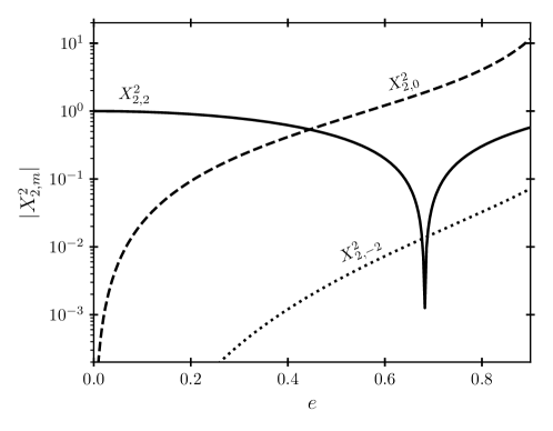
Figure 12 plots the coefficients $|X^{2}_{2,m}|$ relevant for our obliquity integrations. The component $\{k,\ell,m_{\rm orb}\}=\{2,2,2\}$ plotted in Figure 4 couples most strongly with the axisymmetric, $m=0$ mode until the eccentricity exceeds $e\gtrsim 0.4$.

We transform $(x_{\rm orb},y_{\rm orb},z_{\rm orb})$ to a coordinate system with the $z$-axis parallel to ${\bm{\hat{j}}}_{\star}$, and the $y$-axis parallel to ${\bm{\hat{j}}}_{\rm orb}{\bm{\times}}{\bm{\hat{j}}}_{\star}$ (the orbit’s node), co-rotating with the stellar spin. After rotating $Y_{\ell m_{\rm orb}}(\theta_{\rm orb},\varphi_{\rm orb})$ by the Euler angles ($\alpha_{E},\beta_{E},\gamma_{E})=(-\Omega_{\star}t,\psi,\omega_{p}+\pi/2)$, where $\omega_{p}$ is the argument of pericenter, we obtain

$$Y_{\ell m_{\rm orb}}(\theta_{\rm orb},\varphi_{\rm orb})=\sum_{m=-\ell}^{\ell}D^{\ell}_{mm_{\rm orb}}(\alpha_{E},\beta_{E},\gamma_{E})Y_{\ell m}(\theta,\varphi).$$ (A4)

Here, $m$ is the azimuthal number in the star’s rotating frame, and $D^{\ell}_{mm^{\prime}}(\alpha_{E},\beta_{E},\gamma_{E})$ are Wigner $D$-functions using the $z$-$y$-$z$ convention of Varshalovich et al. (1988). Inserting equation (A4) into (A1), we obtain the tidal potential in the star’s rotating frame:

$$U(t,r,\theta,\varphi)=-\frac{GM_{\star}}{R_{\star}}\sum_{k=-\infty}^{\infty}\sum_{\ell=2}^{\infty}\sum_{m=-\ell}^{\ell}\sum_{m_{\rm orb}=-\ell}^{\ell}\left(\frac{r}{R_{\star}}\right)^{\ell}U_{\ell mm_{\rm orb}}^{k}Y_{\ell m}(\theta,\varphi){\rm e}^{-{\rm i}\omega_{km}t},$$ (A5)

where

$$U_{\ell mm_{\rm orb}}^{k}=\frac{M_{\rm p}}{M_{\star}}\left(\frac{R_{\star}}{a}\right)^{\ell+1}Z_{\ell mm_{\rm orb}}^{k},$$ (A6)

$$Z_{\ell mm_{\rm orb}}^{k}(e,\psi,\omega_{p})=W_{\ell m_{\rm orb}}X_{\ell m_{\rm orb}}^{k}(e)d_{mm_{\rm orb}}^{\ell}(\psi){\rm e}^{-{\rm i}m_{\rm orb}(\omega_{p}+\pi/2)},$$ (A7)

$$\omega_{km}=k\Omega-m\Omega_{\star}.$$ (A8)

The Wigner $D$-function is related to the Wigner small-$d$ functions via $D_{mm^{\prime}}^{\ell}(\alpha_{E},\beta_{E},\gamma_{E})={\rm e}^{-{\rm i}\alpha_{E}}d_{mm^{\prime}}^{\ell}(\beta_{E}){\rm e}^{-{\rm i}\gamma_{E}}$. Fixing $\ell=2$, because $W_{\ell m_{\rm orb}}$ is non-zero only for $m_{\rm orb}=\pm 2,0$, the only contributing $d_{mm_{\rm orb}}^{\ell}(\beta_{E})$ values are

$$d^{2}_{\pm 2,2}=\frac{1}{4}(1\pm\cos\beta_{E})^{2}, d^{2}_{\pm 1,2}=\frac{1}{2}\sin\beta_{E}(1\pm\cos\beta_{E}), d^{2}_{0,2}=\sqrt{\frac{3}{8}}\sin^{2}\beta_{E},$$

$$d^{2}_{\pm 2,0}=\sqrt{\frac{3}{8}}\sin^{2}\beta_{E}, d^{2}_{\pm 1,0}=\mp\sqrt{\frac{3}{2}}\sin\beta_{E}\cos\beta_{E}, d^{2}_{0,0}=\frac{1}{2}(3\cos^{2}\beta_{E}-1),$$

$$d^{2}_{\pm 2,-2}=\frac{1}{4}(1\mp\cos\beta_{E})^{2}, d^{2}_{\pm 1,-2}=-\frac{1}{2}\sin\beta_{E}(1\mp\cos\beta_{E}), d^{2}_{0,-2}=\sqrt{\frac{3}{8}}\sin^{2}\beta_{E}.$$ (A9)

A.2 Mode Amplitude

The mode amplitude evolves as (e.g. Schenk et al., 2001; Lai & Wu, 2006)

$$\dot{c}_{\alpha}+({\rm i}\omega_{\alpha}+\gamma_{\alpha})c_{\alpha}={\rm i}\omega_{\alpha}\sum_{k=-\infty}^{\infty}\sum_{\ell=2}^{\infty}\sum_{m=-\ell}^{\ell}\sum_{m_{\rm orb}=-\ell}^{\ell}U_{\ell mm_{\rm orb}}^{k}\left(\frac{E_{\star}}{\varepsilon_{\alpha}}\right)I_{\alpha\ell m}{\rm e}^{-{\rm i}\omega_{km}t},$$ (A10)

where $E_{\star}=GM_{\star}^{2}/R_{\star}$ is the host’s binding energy,

$$\varepsilon_{\alpha}=2\omega_{\alpha}^{2}\int{\bm{\xi}}_{\alpha}^{*}{\bm{\cdot}}{\bm{\xi}}_{\alpha}\rho{\rm d}V$$ (A11)

is the mode energy (added to its complex conjugate), while overlap integral is (e.g. Weinberg et al., 2012)

$$I_{\alpha\ell m}=\frac{1}{MR^{\ell}}\int_{0}^{R_{\star}}r^{\ell+2}\delta\rho_{\alpha\ell m}{\rm d}r.$$ (A12)

Equation (A10) has the inhomogenious solution

$$c_{\alpha}=\sum_{k=-\infty}^{\infty}\sum_{\ell=2}^{\infty}\sum_{m=-\ell}^{\ell}\sum_{m_{\rm orb}=-\ell}^{\ell}c_{\alpha\ell mm_{\rm orb}}^{k}{\rm e}^{-{\rm i}\omega_{km}t}$$ (A13)

in the rotating frame of the star, which transforms to

$$c_{\alpha,{\rm inert}}=\sum_{k=-\infty}^{\infty}\sum_{\ell=2}^{\infty}\sum_{m=-\ell}^{\ell}\sum_{m_{\rm orb}=-\ell}^{\ell}c_{\alpha\ell mm_{\rm orb}}^{k}{\rm e}^{-{\rm i}k\Omega t}$$ (A14)

in the inertial frame, where

$$c_{\alpha\ell mm_{\rm orb}}^{k}=\frac{\omega_{\alpha}}{\omega_{\alpha}-\omega_{km}-{\rm i}\gamma_{\alpha}}U_{\ell mm_{\rm orb}}^{k}\left(\frac{E_{\star}}{\varepsilon_{\alpha}}\right)I_{\alpha\ell m}.$$ (A15)

Notice that when $\omega_{km}\approx\omega_{\alpha}$, a single oscillation $\alpha$ forced by the tidal component $\{k,\ell,m\}$ has an amplitude much larger than other oscillations. For this reason, we will consider a single oscillation $\alpha$ forced by a fixed component of the tidal potential $\{k,\ell,m\}$, and drop subscripts $\{\alpha,k,\ell\}$ on all quantities for the remainder of Appendix A (but keep $\{m,m_{\rm orb}\}$). Also, we will work solely in the inertial frame, and drop the subscript “inert” on equation (A14).

A.3 Energy and Angular Momentum Loss

Equation (A5) shows each tidal component $\{k,\ell,m\}$ is forced by multiple orbital azimuthal numbers $m_{\rm orb}$, each of which differs in phase by $m_{\rm orb}\omega_{p}$. Because we expect short-range forces to cause $\omega_{p}$ to precess over a timescale much shorter than $\sim$1 Gyr (e.g. Liu et al., 2015), we will average over the planet’s argument of pericenter, on top of azimuthal and time averages. Every orbital azimuthal number $m_{\rm orb}$ from an eccentric planet’s tidal potential, forcing a g-mode with azimuthal number $m$, is included in our calculation.

A.3.1 Energy Loss

The energy transferred from the planet’s orbit to the star is (e.g. Lai, 2012):

$$\dot{E}=\int\dot{\bm{\xi}}^{*}{\bm{\cdot}}{\bm{\nabla}}(-U)\rho{\rm d}V=-\int\frac{\partial}{\partial t}\delta\rho^{*}\ U{\rm d}V.$$ (A16)

Inserting equations (A5) and (A14),

$$\dot{E}_{m}={\rm i}\frac{GM^{2}}{a}k\Omega I_{m}^{*}\sum_{m_{\rm orb}=-2}^{2}c_{mm_{\rm orb}}^{*}U_{mm_{\rm orb}}.$$ (A17)

After averaging over $\omega_{p}$, this reduces to

$$\langle\dot{E}_{m}\rangle=\frac{1}{2\pi}\int_{0}^{2\pi}\dot{E}_{m}\ {\rm d}\omega_{p}=\frac{GM_{\star}^{2}}{a}k\Omega\frac{\omega[\gamma+{\rm i}(\omega-\omega_{m})]}{(\omega-\omega_{m})^{2}+\gamma^{2}}(I_{m}^{*})^{2}\left(\frac{E_{\star}}{\varepsilon}\right)\sum_{m_{\rm orb}=-2}^{2}|U_{mm_{\rm orb}}|^{2}.$$ (A18)

A.3.2 Angular Momentum Loss ($z$-direction)

The torque in the $z$-direction is (e.g. Lai, 2012)

$$T_{z}=\int\delta\rho^{*}L_{z}(-U){\rm d}V,$$ (A19)

where

$$L_{z}=\frac{\partial}{\partial\varphi}$$ (A20)

is the z-component of the angular momentum operator. Inserting equation (A5) and averaging over one orbital period, we find

$$T_{z,m}={\rm i}m\left(\frac{GM_{\star}^{2}}{a}\right)\sum_{m_{\rm orb}=-2}^{2}c_{mm_{\rm orb}}^{*}I_{m}^{*}U_{mm_{\rm orb}}.$$ (A21)

Also averaging over $\omega_{p}$, this reduces to

$$\langle T_{z,m}\rangle=\frac{1}{2\pi}\int_{0}^{2\pi}T_{z,m}\ {\rm d}\omega_{p}=\frac{GM_{\star}^{2}}{a}m\frac{\omega[\gamma+{\rm i}(\omega-\omega_{m})]}{(\omega-\omega_{m})^{2}+\gamma^{2}}(I_{m}^{*})^{2}\left(\frac{E_{\star}}{\varepsilon}\right)\sum_{m_{\rm orb}=-2}^{2}|U_{mm_{\rm orb}}|^{2}.$$ (A22)

Notice that

$$\langle T_{z,m}\rangle=\frac{m}{k\Omega}\langle\dot{E}_{m}\rangle,$$ (A23)

as expected (e.g. Schenk et al., 2001).

A.3.3 Angular Momentum Loss ($x$ and $y$ directions)

The torque in the $x$ and $y$ directions are (e.g. Lai, 2012)

$$T_{x}=\int\delta\rho^{*}L_{x}(-U){\rm d}V,\hskip 14.22636ptT_{y}=\int\delta\rho^{*}L_{y}(-U){\rm d}V,$$ (A24)

where

$$L_{x}=-\sin\varphi\frac{\partial}{\partial\theta}-\cot\theta\cos\varphi\frac{\partial}{\partial\varphi},\hskip 14.22636ptL_{y}=\cos\varphi\frac{\partial}{\partial\theta}-\cot\theta\sin\varphi\frac{\partial}{\partial\varphi},$$ (A25)

are the angular momentum operators in the $x$ and $y$ directions. Re-writing these in terms of the raising and lowering operators in quantum mechanics:

$$L_{x}=\frac{1}{2}(L_{+}+L_{-}),\hskip 14.22636ptL_{y}=-\frac{1}{2}{\rm i}(L_{+}-L_{-}),$$ (A26)

where

$$L_{\pm}={\rm i}{\rm e}^{\pm i\varphi}\left(\pm\frac{\partial}{\partial\theta}+{\rm i}\cot\theta\frac{\partial}{\partial\varphi}\right),$$ (A27)

and using the well-known relation with spherical harmonics

$$L_{\pm}Y_{m}={\rm i}\Lambda_{m}^{\pm}Y_{m\pm 1},$$ (A28)

where

$$\Lambda_{m}^{\pm}=\sqrt{\ell(\ell+1)-m(m\pm 1)},$$ (A29)

inserting equation (A5) into $T_{x}$ and $T_{y}$ gives

$$T_{x,m} =\frac{{\rm i}}{2}\left(\frac{GM_{\star}^{2}}{a}\right)I_{m}^{*}\sum_{m_{\rm orb}=-2}^{2}c_{mm_{\rm orb}}^{*}\left[\Lambda_{m}^{+}U_{(m+1)m_{\rm orb}}+\Lambda^{-}_{m}U_{(m-1)m_{\rm orb}}\right],$$ (A30)

$$T_{y,m} =-\frac{1}{2}\left(\frac{GM_{\star}^{2}}{a}\right)I_{m}^{*}\sum_{m_{\rm orb}=-2}^{2}c_{mm_{\rm orb}}^{*}\left[\Lambda_{m}^{+}U_{(m+1)m_{\rm orb}}-\Lambda^{-}_{m}U_{(m-1)m_{\rm orb}}\right].$$ (A31)

Averaging $T_{x,m}$ and $T_{y,m}$ over $\omega_{p}$, we may write

$$\langle T_{x,m}\rangle =\frac{1}{2\pi}\int_{0}^{2\pi}T_{x,m}\ {\rm d}\omega_{p}=\frac{1}{2m}\left(\tau_{m}^{+}+\tau_{m}^{-}\right)\langle T_{z,m}\rangle=\frac{1}{2k\Omega}\left(\tau_{m}^{+}+\tau_{m}^{-}\right)\langle\dot{E}_{m}\rangle,$$ (A32)

$$\langle T_{y,m}\rangle =\frac{1}{2\pi}\int_{0}^{2\pi}T_{y,m}\ {\rm d}\omega_{p}=\frac{{\rm i}}{2m}\left(\tau_{m}^{+}-\tau_{m}^{-}\right)\langle T_{z,m}\rangle=\frac{{\rm i}}{2k\Omega}\left(\tau_{m}^{+}-\tau_{m}^{-}\right)\langle\dot{E}_{m}\rangle,$$ (A33)

where

$$\tau_{m}^{\pm}=\left[\sum_{m_{\rm orb}=-2}^{2}\Lambda_{m}^{\pm}Z_{(m\pm 1)m_{\rm orb}}Z_{mm_{\rm orb}}\right]\Bigg{/}\left[\sum_{m_{\rm orb}=-2}^{2}|Z_{mm_{\rm orb}}|^{2}\right]$$ (A34)

We will neglect $T_{y}$ in this work, as this causes precession of the spin axis about the orbit normal.

A.4 Orbital evolution for arbitrary resonance

Now, consider an oscillation frequency in the inertial frame $\sigma$ (mode index $\alpha$, and angular/azumuthal number $\ell$, $m$ suppressed). Resonance locking occurs when an integer harmonic $k$ of the orbital frequency satisfies

$$k\Omega\simeq\sigma.$$ (A35)

Differentiating with time and re-arranging, one can show in the absence of other forces (e.g. magnetic breaking, contraction, additional planet/star tides), that (Fuller, 2017)

$$t_{\rm ev}^{-1}\equiv\frac{\dot{\sigma}}{\sigma}=\eta\frac{\dot{E}_{\rm orb}}{E_{\rm orb}},$$ (A36)

where

$$\eta=\frac{3}{2}-\frac{m^{2}B}{2k^{2}\sqrt{1-e^{2}}}\left(\frac{M_{\rm p}a^{2}}{\kappa_{\star}M_{\star}R_{\star}^{2}}\right),$$ (A37)

and (assuming $\Omega_{\star}\ll\sigma$)

$$B=\frac{1}{m}\frac{\partial\sigma}{\partial\Omega_{\star}}\simeq 1-\frac{1}{\ell(\ell+1)}.$$ (A38)

Inserting the averaged equations (A23) and (A32) into (1)-(4), and re-arranging $\dot{J}_{\rm orb}$ and $\dot{E}_{\rm orb}$ to get ${\rm d}e/{\rm d}t$, we find

$$\frac{1}{a}\frac{{\rm d}a}{{\rm d}t}= -\frac{1}{\eta t_{\rm ev}},$$ (A39)

$$\frac{{\rm d}J_{\star}}{{\rm d}t}= \ \frac{m}{2k\sqrt{1-e^{2}}}\frac{J_{\rm orb}}{\eta t_{\rm ev}},$$ (A40)

$$\frac{{\rm d}e}{{\rm d}t}= -\frac{1-e^{2}}{2e}\bigg{[}1-\frac{1}{k\sqrt{1-e^{2}}}\left(\tau_{m}\sin\psi+m\cos\psi\right)\bigg{]}\frac{1}{\eta t_{\rm ev}},$$ (A41)

$$\frac{{\rm d}\psi}{{\rm d}t}= -\frac{1}{2k\sqrt{1-e^{2}}}\bigg{[}\tau_{m}\left(\frac{J_{\rm orb}}{J_{\star}}+\cos\psi\right)-m\sin\psi\bigg{]}\frac{1}{\eta t_{\rm ev}},$$ (A42)

where

$$\tau_{m}=\frac{\tau_{m}^{+}+\tau_{m}^{-}}{2}=\frac{m\langle T_{x,m}\rangle}{\langle T_{z,m}\rangle}=\frac{k\Omega\langle T_{x,m}\rangle}{\langle\dot{E}_{m}\rangle}.$$ (A43)

Depending on the eccentricity and obliquity, these equations predict the eccentricity and obliquity can damp or grow.

Appendix B Gravity Mode Dissipation

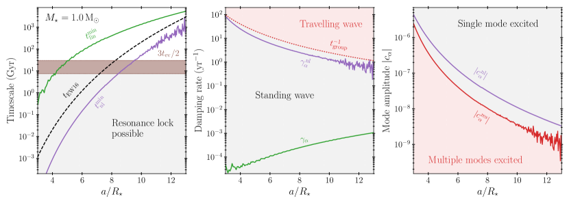
Resonance locking cannot operate out to arbitrarily large $a/R_{\star}$: when $a/R_{\star}$ is larger than a critical distance $(a/R_{\star})_{\rm crit}$, the g-mode dissipation is too weak, and resonances sweep by the planet’s orbit. Specifically, the timescale resonance locking evolves the semi-major axis at, $3t_{\rm ev}/2$, must be longer than the orbital energy dissipation timescale close to resonance $t_{\rm mode}^{\rm min}=|E_{\rm orb}({\rm d}E_{\rm mode}/{\rm d}t)^{-1}|$ (e.g. Zanazzi & Wu, 2021). This appendix section estimates $(a/R_{\star})_{\rm crit}$ for hot Jupiter systems, considering the different ways a g-mode can dissipate energy. We find it necessary to invoke non-linear g-mode dissipation to damp obliquities of cool stars out to $a/R_{\star}\sim 8$, and emphasize that our estimates are highly uncertain. However, we verify that our estimates for g-modes undergoing non-linear dissipation behave like a single, resonantly-excited standing wave: our non-linear damping rates have magnitudes less than the inverse of the group travel time, and only one g-mode will be excited to non-linear amplitudes.

We first estimate the rate of energy dissipation from a standing mode which damps due to radiative diffusion. We use the stellar oscillation code GYRE to calculate g-mode properties with a solar mass star background MESA model at 4 Gyr, with damping rates $\gamma_{\alpha}$ evaluated using the GYRE inlists in Fuller (2017). Writing the the mode displacement ${\bm{\xi}}(t,{\bm{r}})=c_{\alpha}(t){\bm{\xi}}_{\alpha}({\bm{r}})$, with the eigenmode ${\bm{\xi}}_{\alpha}$ and eigenfrequency $\omega_{\alpha}$ normalized so that its energy $\varepsilon_{\alpha}=E_{\star}$ (e.g. Schenk et al., 2001; Lai & Wu, 2006), the orbital energy dissipation timescale near resonance is given by

$$t_{\rm lin}^{\rm min}=\frac{|E_{\rm orb}|}{2\gamma_{\alpha}|c_{\alpha}^{\rm max}|^{2}E_{\star}},$$ (B1)

where $\gamma_{\alpha}>0$ denotes mode damping, and $c_{\alpha}^{\rm max}$ is the maximum amplitude of the mode. Equation (B1) is valid near a g-mode resonance, or when Coriolis forces are negligible, see Dewberry & Wu (2024) for corrections when these assumptions break down. If the mode remains everywhere linear, $c_{\alpha}^{\rm max}$ is set by balancing the tidal driving with the mode damping (e.g. Zanazzi & Wu, 2021; Ma & Fuller, 2021). However, stratification in the radiative cores of low-mass stars can cause the mode to become highly non-linear. Denoting $\xi_{r}=\iint{\bm{\xi}}_{\alpha}{\bm{\cdot}}{\bm{\hat{r}}}Y_{\ell m}^{*}\sin\theta\,{\rm d}\theta\,{\rm d}\varphi$, standing waves must satisfy

$$\left|\frac{{\rm d}\xi_{r}}{{\rm d}r}\right|=c_{\alpha}\left|\frac{{\rm d}\xi_{r,\alpha}}{{\rm d}r}\right|\lesssim 1,$$ (B2)

otherwise the wave to overturns and breaks (e.g. Goodman & Dickson, 1998; Barker & Ogilvie, 2010, 2011; Barker, 2011; Guo et al., 2023). We set

$$c_{\alpha}^{\rm max}=\left|\frac{{\rm d}\xi_{r,\alpha}}{{\rm d}r}\right|^{-1}_{\rm max},$$ (B3)

where $|{\rm d}\xi_{r,\alpha}/{\rm d}r|_{\rm max}$ is the maximum magnitude of ${\rm d}\xi_{r,\alpha}/{\rm d}r$ over the star’s radial extent, typically near the mode’s turning point $r_{m}$ close to the star’s center (where $N(r_{m})=\omega_{\alpha}$, e.g. Goodman & Dickson, 1998; Zanazzi & Wu, 2021). Examining Figure  13, linear dissipation of g-modes can only cause resonance locking out to $(a/R_{\star})_{\rm crit}\approx 4-5$.

Figure 13: Left panel: Migration timescales at resonance ($\omega_{\alpha}=2\Omega$), for a solar-mass 4 Gyr old star. The range of $t_{\rm ev}$ values is lifted from Fig. 6. Linear damping from radiative diffusion $t_{\rm lin}^{\rm min}$ (eq. B1) can damp obliquities out to $(a/R_{\star})_{\rm crit}\approx 4-5$, while non-linear coupling $t_{\rm nl}^{\rm min}$ (eq. B5) works to $(a/R_{\star})_{\rm crit}\approx 8-9$. The non-linear migration timescale $t_{\rm EW16}$ (eq. B7) from Essick & Weinberg (2016) is plotted for comparison. Middle panel: Linear damping from GYRE $\gamma_{\alpha}$, and non-linear damping $\gamma_{\alpha}^{\rm nl}$ from equation (B4). For standing waves to travel from the center to the surface, damping must be less than $t_{\rm group}^{-1}$ (eq. B10), satisfied for linear $\gamma_{\alpha}$ and non-linear $\gamma_{\alpha}^{\rm nl}$ damping. Right panel: Non-linear saturation amplitude $c_{\alpha}^{\rm nl}$ (eq. B6), compared with the linear resonant amplitude $c_{\alpha}^{\rm res}$ (eq. B11). For a single, resonant mode to be non-linearly excited and saturate, we require $|c_{\alpha}^{\rm nl}|\gtrsim|c_{\alpha}^{\rm res}|$.

However, as the g-mode grows in amplitude, a parametric instability can modify its buoyant restoring force, and increase its dissipation rate (e.g. Kumar & Goodman, 1996; Wu & Goldreich, 2001; Weinberg et al., 2023; Van Beeck et al., 2023). This parametric instability should saturate the g-mode amplitude at a value $c_{\alpha}\approx c_{\alpha}^{\rm nl}$, when the growth rate of the instability $\gamma_{\alpha}^{\rm nl}$ matches the frequency shift of the oscillation $|\omega_{\alpha}^{\rm nl}-2\Omega|$ (see e.g. appendix C of Kumar & Goodman 1996). Replacing $\omega_{\alpha}$ and $\gamma_{\alpha}$ with $\omega_{\alpha}^{\rm nl}$ and $\gamma_{\alpha}^{\rm nl}$ in equation (A15), $\gamma_{\alpha}^{\rm nl}$ can be written in terms of the tidal driving and the saturation amplitude $c_{\alpha}^{\rm nl}$:

$$\gamma_{\alpha}^{\rm nl}\approx|\omega_{\alpha}^{\rm nl}-2\Omega|\approx\frac{\omega_{\alpha}|I_{\alpha 20}|}{|c_{\alpha}^{\rm nl}|}|U^{2}_{202}|.$$ (B4)

We have assumed the planet’s orbit is circular, with $U^{k}_{\ell mm_{\rm orb}}$ given by equation (A6), and added $c_{\alpha}$ to its complex conjugate. Near resonance ($\omega_{\alpha}\approx\omega_{\alpha}^{\rm nl}\approx 2\Omega)$, the timescale this parametric instability extracts energy from the orbit is then

$$t_{\rm nl}^{\rm min}\approx\frac{|E_{\rm orb}|}{2\gamma_{\alpha}^{\rm nl}|c_{\alpha}^{\rm nl}|^{2}E_{\star}}.$$ (B5)

Figure 13 compares (B5) to $3t_{\rm ev}/2$, assuming a Jovian-mass planet on a circular orbit, with obliquity $\psi=90^{\circ}$. We have parameterized $c_{\alpha}^{\rm nl}$ in terms of the mode’s non-linear amplitude

$$|c_{\alpha}^{\rm nl}|\approx\Xi\left|\frac{{\rm d}\xi_{r,\alpha}}{{\rm d}r}\right|^{-1}_{\rm max},$$ (B6)

and taken $\Xi=0.1$, motivated by hydrodynamical simulations which show standing waves saturate and break when $|{\rm d}\xi_{r}/{\rm d}r|\sim 0.1$ (see Guo et al., 2023, Figs. 4 & 23). Lower values of $\Xi$ predict higher values of $\gamma_{\alpha}^{\rm nl}$. We compare our $t_{\rm nl}^{\rm min}$ estimate to that of Essick & Weinberg (2016):

$$t_{\rm EW16}=4.1\times 10^{7}\left(\frac{P_{\rm orb}}{{\rm day}}\right)^{6.7}{\rm yr}.$$ (B7)

Although our $t_{\rm nl}^{\rm min}$ estimate is lower than Essick & Weinberg (2016) by a factor of a few, the scaling with $a/R_{\star}$ is very similar. Both estimates agree $t_{\rm nl}^{\rm min}$ is smaller than $3t_{\rm ev}/2$ out to $(a/R_{\star})_{\rm crit}\approx 6-9$.

Section 4 assumed resonance locks could be sustained until the stellar spin aligns with the planet’s orbit normal, evolving the orbit until $\psi\to 0$. However, if the obliquity crosses a threshold value $\psi_{\rm break}$, or the obliquity where $t_{\rm mode}^{\rm min}=t_{\rm lin}^{\rm lin},t_{\rm nl}^{\rm min}=3t_{\rm ev}/2$, the resonance lock breaks. For g-mode damping from radiative diffusion, the dissipation rate $\gamma_{\alpha}$ is set by properties of the standing mode, while $c_{\alpha}^{\rm max}$ mainly depends on the core’s stratification. Hence, $t_{\rm lin}^{\rm min}$ is independent of $\psi$ for low-mass stars:

$$\psi_{\rm break}^{\rm lin}\approx 0^{\circ}\text{ when }t_{\rm lin}^{\rm min}\lesssim 3t_{\rm ev}/2,\hskip 14.22636pt\psi_{\rm break}^{\rm lin}\approx 180^{\circ}\text{ when }t_{\rm lin}^{\rm min}\gtrsim 3t_{\rm ev}/2,$$ (B8)

The green region in Figure 11 displays where $t_{\rm lin}^{\rm min}=3t_{\rm ev}/2$, taking $t_{\rm lin}^{\rm min}$ from Figure 13, for a range of $t_{\rm ev}$ values characteristic of main-sequence stars below the Kraft break (Fig. 6). Resonance locking will damp obliquities to zero interior to $(a/R_{\star})_{\rm crit}\sim 4-5$. If the initial distributions of low and high-mass star obliquities are similar before tides can differentiate them, mode damping from radiative diffusion appears insufficient to re-align most cool stars hosting hot Jupiters out to $(a/R_{\star})\sim 6-10$.

Because the parametric instability will increase the orbital energy dissipation rate, it predicts $\psi_{\rm break}>0^{\circ}$ to larger $a/R_{\star}$. By construction, our parameterized saturation amplitude $c_{\alpha}^{\rm nl}$ depends mainly on the core’s stratification (eq. B6). However, the non-linear damping rate $\gamma_{\alpha}^{\rm nl}\propto|U_{202}^{2}|\propto\sin^{2}\psi$ (eq. B4), therefore

$$|\sin\psi_{\rm break}^{\rm nl}|\approx\left(\frac{2t^{\rm min}_{{\rm nl},\psi=90^{\circ}}}{3t_{\rm ev}}\right)^{1/2}\text{ when }t_{{\rm nl},\psi=90^{\circ}}^{\rm min}\lesssim 3t_{\rm ev}/2.$$ (B9)

The purple curves in Figure 11 display equation (B9), taking $t^{\rm min}_{{\rm nl},\psi=90^{\circ}}$ from Figure 13, with $t_{\rm ev}$ from Figure 6. In contrast with linear damping, non-linear dissipation could explain the low obliquities of cool stars out to $(a/R_{\star})_{\rm crit}\sim 8$.

For g-modes undergoing linear or non-linear dissipation to behave like standing waves, they must be able to propagate from the star’s center to surface without suffering significant damping. This requires a damping rate smaller than the group travel time (e.g. Goodman & Dickson, 1998; Zanazzi & Wu, 2021; Ma & Fuller, 2021)

$$t_{\rm group}\simeq\frac{\pi n}{\omega_{\alpha}},$$ (B10)

otherwise the oscillation becomes a travelling wave. This is well-satisfied for linear, and marginally-satisfied for non-linear, damping (Fig. 13).

Resonance locking relies on only one oscillation being excited by the tidal potential. For non-linear damping to saturate one, and only one, oscillation, neighboring oscillations must have amplitudes less than $c_{\alpha}^{\rm nl}$. Tidal forcing excites neighbors to a maximum amplitude of (eq. A15)

$$c_{\alpha}^{\rm res}\approx\left(\frac{2}{\Delta\omega_{\alpha}}\right)\omega_{\alpha}U^{2}_{202}I_{\alpha 20}\approx 2nU^{2}_{202}I_{\alpha 20},$$ (B11)

assuming the spacing between oscillations $\Delta\omega_{\alpha}\approx\omega_{\alpha}/n$. Figure 13 shows $|c_{\alpha}^{\rm nl}|$ is larger than $|c_{\alpha}^{\rm res}|$ by a factor of $\sim$2-4.

The semi-analytic calculations of Essick & Weinberg (2016) found weak non-linearities caused tidal dissipation to increase by a factor $\lesssim$2 near a g-mode oscillation. If one instead takes $\Xi\lesssim 0.05$, as suggested by their work (e.g. Essick & Weinberg, 2016, their eqs. 79, 80 in appendix F), multiple neighboring resonances can become saturated ($|c_{\alpha}^{\rm nl}|\gtrsim|c_{\alpha}^{\rm res}|$), and g-modes can become travelling waves ($\gamma_{\alpha}^{\rm nl}\gtrsim t_{\rm group}^{-1}$). Hot Jupiters no longer have to “wait” for a resonance to lock onto their orbit, so $3t_{\rm ev}/2$ in equations (A39)-(A42) is replaced by $t_{\rm EW16}$ (eq. B7). The timescale low-mass stars damp their obliquities will then be shorter (Fig. 13). Moreover, because multiple oscillations are now excited, one sums equations (A39)-(A42) over all $k$ and $m$. However, saturated locks will also have shorter orbital migration timescales, possibly in-spiraling into the star or becoming tidally disrupted before the obliquity is fully damped. The non-linear saturation of tidally-forced g-modes will be investigated in a future work.

References

- Albrecht et al. (2012) Albrecht, S., Winn, J. N., Johnson, J. A., et al. 2012, ApJ, 757, 18, doi: 10.1088/0004-637X/757/1/18
- Albrecht et al. (2022) Albrecht, S. H., Dawson, R. I., & Winn, J. N. 2022, PASP, 134, 082001, doi: 10.1088/1538-3873/ac6c09
- Albrecht et al. (2021) Albrecht, S. H., Marcussen, M. L., Winn, J. N., Dawson, R. I., & Knudstrup, E. 2021, ApJ, 916, L1, doi: 10.3847/2041-8213/ac0f03
- Anderson et al. (2021) Anderson, K. R., Winn, J. N., & Penev, K. 2021, ApJ, 914, 56, doi: 10.3847/1538-4357/abf8af
- Astropy Collaboration et al. (2013) Astropy Collaboration, Robitaille, T. P., Tollerud, E. J., et al. 2013, A&A, 558, A33, doi: 10.1051/0004-6361/201322068
- Astropy Collaboration et al. (2018) Astropy Collaboration, Price-Whelan, A. M., Sipőcz, B. M., et al. 2018, AJ, 156, 123, doi: 10.3847/1538-3881/aabc4f
- Barker (2011) Barker, A. J. 2011, MNRAS, 414, 1365, doi: 10.1111/j.1365-2966.2011.18468.x
- Barker & Astoul (2021) Barker, A. J., & Astoul, A. A. V. 2021, MNRAS, 506, L69, doi: 10.1093/mnrasl/slab077
- Barker & Ogilvie (2009) Barker, A. J., & Ogilvie, G. I. 2009, MNRAS, 395, 2268, doi: 10.1111/j.1365-2966.2009.14694.x
- Barker & Ogilvie (2010) —. 2010, MNRAS, 404, 1849, doi: 10.1111/j.1365-2966.2010.16400.x
- Barker & Ogilvie (2011) —. 2011, MNRAS, 417, 745, doi: 10.1111/j.1365-2966.2011.19322.x
- Damiani & Mathis (2018) Damiani, C., & Mathis, S. 2018, A&A, 618, A90, doi: 10.1051/0004-6361/201732538
- Dawson (2014) Dawson, R. I. 2014, ApJ, 790, L31, doi: 10.1088/2041-8205/790/2/L31
- Dawson & Johnson (2018) Dawson, R. I., & Johnson, J. A. 2018, ARA&A, 56, 175, doi: 10.1146/annurev-astro-081817-051853
- Dewberry & Wu (2024) Dewberry, J. W., & Wu, S. C. 2024, MNRAS, 527, 2288, doi: 10.1093/mnras/stad3164
- Dong & Foreman-Mackey (2023) Dong, J., & Foreman-Mackey, D. 2023, AJ, 166, 112, doi: 10.3847/1538-3881/ace105
- Espinoza-Retamal et al. (2023) Espinoza-Retamal, J. I., Brahm, R., Petrovich, C., et al. 2023, ApJ, 958, L20, doi: 10.3847/2041-8213/ad096d
- Essick & Weinberg (2016) Essick, R., & Weinberg, N. N. 2016, ApJ, 816, 18, doi: 10.3847/0004-637X/816/1/18
- Fabrycky & Winn (2009) Fabrycky, D. C., & Winn, J. N. 2009, ApJ, 696, 1230, doi: 10.1088/0004-637X/696/2/1230
- Fuller (2017) Fuller, J. 2017, MNRAS, 472, 1538, doi: 10.1093/mnras/stx2135
- Goldreich & Nicholson (1977) Goldreich, P., & Nicholson, P. D. 1977, Icarus, 30, 301, doi: 10.1016/0019-1035(77)90163-4
- Goldstein & Townsend (2020) Goldstein, J., & Townsend, R. H. D. 2020, ApJ, 899, 116, doi: 10.3847/1538-4357/aba748
- Goodman & Dickson (1998) Goodman, J., & Dickson, E. S. 1998, ApJ, 507, 938, doi: 10.1086/306348
- Guillochon et al. (2011) Guillochon, J., Ramirez-Ruiz, E., & Lin, D. 2011, ApJ, 732, 74, doi: 10.1088/0004-637X/732/2/74
- Guo et al. (2023) Guo, Z., Ogilvie, G. I., & Barker, A. J. 2023, MNRAS, 521, 1353, doi: 10.1093/mnras/stad569
- Hamer & Schlaufman (2022) Hamer, J. H., & Schlaufman, K. C. 2022, AJ, 164, 26, doi: 10.3847/1538-3881/ac69ef
- Harris et al. (2020) Harris, C. R., Millman, K. J., van der Walt, S. J., et al. 2020, Nature, 585, 357, doi: 10.1038/s41586-020-2649-2
- Hébrard et al. (2011) Hébrard, G., Ehrenreich, D., Bouchy, F., et al. 2011, A&A, 527, L11, doi: 10.1051/0004-6361/201016331
- Henyey et al. (1955) Henyey, L. G., Lelevier, R., & Levée, R. D. 1955, PASP, 67, 154, doi: 10.1086/126791
- Hu et al. (2024) Hu, Q., Rice, M., Wang, X.-Y., et al. 2024, arXiv e-prints, arXiv:2402.07346, doi: 10.48550/arXiv.2402.07346
- Jermyn et al. (2023) Jermyn, A. S., Bauer, E. B., Schwab, J., et al. 2023, ApJS, 265, 15, doi: 10.3847/1538-4365/acae8d
- Kumar & Goodman (1996) Kumar, P., & Goodman, J. 1996, ApJ, 466, 946, doi: 10.1086/177565
- Lai (2012) Lai, D. 2012, MNRAS, 423, 486, doi: 10.1111/j.1365-2966.2012.20893.x
- Lai & Wu (2006) Lai, D., & Wu, Y. 2006, Phys. Rev. D, 74, 024007, doi: 10.1103/PhysRevD.74.024007
- Li & Winn (2016) Li, G., & Winn, J. N. 2016, ApJ, 818, 5, doi: 10.3847/0004-637X/818/1/5
- Lin & Ogilvie (2017) Lin, Y., & Ogilvie, G. I. 2017, MNRAS, 468, 1387, doi: 10.1093/mnras/stx540
- Liu et al. (2015) Liu, B., Muñoz, D. J., & Lai, D. 2015, MNRAS, 447, 747, doi: 10.1093/mnras/stu2396
- Louden et al. (2021) Louden, E. M., Winn, J. N., Petigura, E. A., et al. 2021, AJ, 161, 68, doi: 10.3847/1538-3881/abcebd
- Ma & Fuller (2021) Ma, L., & Fuller, J. 2021, ApJ, 918, 16, doi: 10.3847/1538-4357/ac088e
- Morgan et al. (2024) Morgan, M., Bowler, B. P., Tran, Q. H., et al. 2024, AJ, 167, 48, doi: 10.3847/1538-3881/ad0728
- Muñoz & Perets (2018) Muñoz, D. J., & Perets, H. B. 2018, AJ, 156, 253, doi: 10.3847/1538-3881/aae7d0
- Paxton et al. (2011) Paxton, B., Bildsten, L., Dotter, A., et al. 2011, ApJS, 192, 3, doi: 10.1088/0067-0049/192/1/3
- Paxton et al. (2013) Paxton, B., Cantiello, M., Arras, P., et al. 2013, ApJS, 208, 4, doi: 10.1088/0067-0049/208/1/4
- Paxton et al. (2015) Paxton, B., Marchant, P., Schwab, J., et al. 2015, ApJS, 220, 15, doi: 10.1088/0067-0049/220/1/15
- Paxton et al. (2018) Paxton, B., Schwab, J., Bauer, E. B., et al. 2018, ApJS, 234, 34, doi: 10.3847/1538-4365/aaa5a8
- Paxton et al. (2019) Paxton, B., Smolec, R., Schwab, J., et al. 2019, ApJS, 243, 10, doi: 10.3847/1538-4365/ab2241
- Penev et al. (2018) Penev, K., Bouma, L. G., Winn, J. N., & Hartman, J. D. 2018, AJ, 155, 165, doi: 10.3847/1538-3881/aaaf71
- Press & Teukolsky (1977) Press, W. H., & Teukolsky, S. A. 1977, ApJ, 213, 183, doi: 10.1086/155143
- Rice et al. (2022a) Rice, M., Wang, S., & Laughlin, G. 2022a, ApJ, 926, L17, doi: 10.3847/2041-8213/ac502d
- Rice et al. (2022b) Rice, M., Wang, S., Wang, X.-Y., et al. 2022b, AJ, 164, 104, doi: 10.3847/1538-3881/ac8153
- Rogers & Lin (2013) Rogers, T. M., & Lin, D. N. C. 2013, ApJ, 769, L10, doi: 10.1088/2041-8205/769/1/L10
- Savonije (2008) Savonije, G. J. 2008, in EAS Publications Series, Vol. 29, EAS Publications Series, ed. M. J. Goupil & J. P. Zahn, 91–125, doi: 10.1051/eas:0829003
- Schenk et al. (2001) Schenk, A. K., Arras, P., Flanagan, É. É., Teukolsky, S. A., & Wasserman, I. 2001, Phys. Rev. D, 65, 024001, doi: 10.1103/PhysRevD.65.024001
- Schlaufman (2010) Schlaufman, K. C. 2010, ApJ, 719, 602, doi: 10.1088/0004-637X/719/1/602
- Sedaghati et al. (2023) Sedaghati, E., Jordán, A., Brahm, R., et al. 2023, AJ, 166, 130, doi: 10.3847/1538-3881/acea84
- Siegel et al. (2023) Siegel, J. C., Winn, J. N., & Albrecht, S. H. 2023, ApJ, 950, L2, doi: 10.3847/2041-8213/acd62f
- Spalding & Winn (2022) Spalding, C., & Winn, J. N. 2022, ApJ, 927, 22, doi: 10.3847/1538-4357/ac4993
- Sullivan & Kaszynski (2019) Sullivan, C. B., & Kaszynski, A. 2019, Journal of Open Source Software, 4, 1450, doi: 10.21105/joss.01450
- Terquem (2021) Terquem, C. 2021, MNRAS, 503, 5789, doi: 10.1093/mnras/stab224
- Townsend et al. (2018) Townsend, R. H. D., Goldstein, J., & Zweibel, E. G. 2018, MNRAS, 475, 879, doi: 10.1093/mnras/stx3142
- Townsend & Teitler (2013) Townsend, R. H. D., & Teitler, S. A. 2013, MNRAS, 435, 3406, doi: 10.1093/mnras/stt1533
- Valsecchi & Rasio (2014) Valsecchi, F., & Rasio, F. A. 2014, ApJ, 786, 102, doi: 10.1088/0004-637X/786/2/102
- Van Beeck et al. (2023) Van Beeck, J., Van Hoolst, T., Aerts, C., & Fuller, J. 2023, arXiv e-prints, arXiv:2311.02972, doi: 10.48550/arXiv.2311.02972
- Varshalovich et al. (1988) Varshalovich, D. A., Moskalev, A. N., & Khersonskii, V. K. 1988, Quantum Theory of Angular Momentum (World Scientific Publishing), doi: 10.1142/0270
- Vick et al. (2019) Vick, M., Lai, D., & Anderson, K. R. 2019, MNRAS, 484, 5645, doi: 10.1093/mnras/stz354
- Vidal & Barker (2020) Vidal, J., & Barker, A. J. 2020, ApJ, 888, L31, doi: 10.3847/2041-8213/ab6219
- Virtanen et al. (2020) Virtanen, P., Gommers, R., Oliphant, T. E., et al. 2020, Nature Methods, 17, 261, doi: 10.1038/s41592-019-0686-2
- Weinberg et al. (2012) Weinberg, N. N., Arras, P., Quataert, E., & Burkart, J. 2012, ApJ, 751, 136, doi: 10.1088/0004-637X/751/2/136
- Weinberg et al. (2023) Weinberg, N. N., Davachi, N., Essick, R., et al. 2023, arXiv e-prints, arXiv:2305.11974, doi: 10.48550/arXiv.2305.11974
- Wes McKinney (2010) Wes McKinney. 2010, in Proceedings of the 9th Python in Science Conference, ed. Stéfan van der Walt & Jarrod Millman, 56 – 61, doi: 10.25080/Majora-92bf1922-00a
- Winn et al. (2010) Winn, J. N., Fabrycky, D., Albrecht, S., & Johnson, J. A. 2010, ApJ, 718, L145, doi: 10.1088/2041-8205/718/2/L145
- Winn et al. (2017) Winn, J. N., Petigura, E. A., Morton, T. D., et al. 2017, AJ, 154, 270, doi: 10.3847/1538-3881/aa93e3
- Witte & Savonije (1999) Witte, M. G., & Savonije, G. J. 1999, A&A, 350, 129, doi: 10.48550/arXiv.astro-ph/9909073
- Witte & Savonije (2001) —. 2001, A&A, 366, 840, doi: 10.1051/0004-6361:20000245
- Wu (2018) Wu, Y. 2018, AJ, 155, 118, doi: 10.3847/1538-3881/aaa970
- Wu & Goldreich (2001) Wu, Y., & Goldreich, P. 2001, ApJ, 546, 469, doi: 10.1086/318234
- Xue et al. (2014) Xue, Y., Suto, Y., Taruya, A., et al. 2014, ApJ, 784, 66, doi: 10.1088/0004-637X/784/1/66
- Zanazzi & Wu (2021) Zanazzi, J. J., & Wu, Y. 2021, AJ, 161, 263, doi: 10.3847/1538-3881/abf097