Information divergences to parametrize astrophysical uncertainties in dark matter direct detection

Abstract

Astrophysical uncertainties in dark matter direct detection experiments are typically addressed by parametrizing the velocity distribution in terms of a few uncertain parameters that vary around some central values. Here we propose a method to optimize over all velocity distributions lying within a given distance measure from a central distribution. We discretize the dark matter velocity distribution as a superposition of streams, and use a variety of information divergences to parametrize its uncertainties. With this, we bracket the limits on the dark matter-nucleon and dark matter-electron scattering cross sections, when the true dark matter velocity distribution deviates from the commonly assumed Maxwell-Boltzmann form. The methodology pursued is general and could be applied to other physics scenarios where a given physical observable depends on a function that is uncertain.

1 Introduction

In the theoretical description of many physical processes, an observable $F$ is a functional of an input function $f$, $F[f]$. For example, the dark matter scattering rate in a direct detection experiment is a functional of the local dark matter velocity distribution; or the gamma-ray/neutrino flux at Earth from dark matter annihilation in the Universe is a functional of the dark matter density distribution. The function $f$ may be calculated from first principles, or be determined from experiments. In either case, it is subject to theoretical and experimental uncertainties, that impact the theoretical prediction of the observable $F[f]$.

In order to bracket the uncertainty in the theoretical prediction of $F[f]$, it is common in the literature to parametrize $f$ in terms of a number of parameters, that vary around some central values. We propose an alternative which consists in using methods of convex optimization to optimize over all functions lying within a given distance measure from a central function, see Fig 1. As distance measures to parametrize the deviation from the distribution, we use information divergences, widely used in mathematics and statistics to quantify differences between probability distributions [1, 2, 3].

Figure 1: The blue lines represent the family of functions obtained by varying the function parameters $\alpha$ and $\beta$ around a central value. The magenta line represents a function that deviates at most a certain value $\Delta$ from the central value of the function $f_{0}$, given a distance measure $D$ parametrizing the deviation among the two functions. It can be clearly seen that varying the parameters $\alpha,\beta$ of the central function $f_{0}$ wouldn’t capture the parametric form of the function $f$.

In particular, the method that we propose consists in optimizing the functional $F$ under some given constraints on $f$, among which one sets a maximal distance $\Delta$ between the central function $f_{0}$ and the optimal function $f$, $D(f,f_{0})\leq\Delta$, given by information divergences. The problems of this class are not always convex neither simple to solve while guaranteeing that the found optimal solution is global. Nonetheless, many of these problems fall in some of the categories of convex problems such as linear programming (LP), quadratic programming (QP), second oder cone programming (SOCP), semi-definite programming (SDP), or exponential programming (EXP) [4]. There are a variety of convex optimization softwares able to formulate and solve these problems with interior-point methods. A very compelling example is CVXPY [5], since it embeds different codes with a narrower applicability to provide a software able to identify and solve a large number of convex optimization problems, via disciplined convex programming [6].

We develop a methodology that allows to bracket the impact of theoretical uncertainties in a given experiment by making use of information divergences and convex optimization techniques, and apply our method to the field of direct dark matter searches. In direct dark matter searches, the rate of dark matter induced scatterings in a detector is a functional of the dark matter velocity distribution. The form of the dark matter velocity distribution, which is as of today unknown, plays a crucial role when interpreting direct dark matter searches. In order to interpret the outcome of direct dark matter searches, one usually assumes the Standard Halo Model. On the other hand, several works showed that deviations from the SHM are expected to be sizable, having an impact in nuclear recoil searches, E.g [7, 8, 9, 10, 11, 12, 13, 14, 15, 16, 17, 18, 19], in electron recoil searches, E.g [20, 21, 22, 23, 24, 17, 18], and in plasmon-induced effects [25, 26]. This source of uncertainty has been treated with analysis frameworks to interpret direct dark matter searches with halo-independent methods and more sophisticated integration techniques [27, 28, 29, 30, 31, 32, 33, 34, 35, 36, 37, 38, 39, 40, 41, 42, 43, 44, 45, 46, 47, 48, 49].

The paper is organized as follows. In section 2 we describe the mathematical form of the optimization problem that we aim to solve. In section 3 we introduce a zoo of distance measures used to parametrize the uncertainties on the dark matter velocity distribution. In section 4, we quantify the deviations from the SHM for different distance measures and models of the dark matter velocity distribution present in the literature. In section 5, we derive upper limits for nuclear recoil searches for different choices of the distance measure. In section 6 we derive upper limits for electron recoil searches for different choices of the distance measure, and study the projected complementarity of XENON1T and SENSEI in the hypothetical scenario that one experiment claims a detection while the other does not. In particular, we quantify the compatibility of a positive signal in one experiment and a null signal in the other when the dark matter velocity distribution deviates from the Maxwell-Boltzmann a maximum value.

2 Functional optimization

We consider the objective functional $\mathcal{F}[f]$ with $f$ a real function with domain $S$. In some physical applications, one aims to find maximum and minimum value of the objective functional $\mathcal{F}$, subject to a number of constraints that are also functionals of $f$. Specifically, the optimization problem can be formulated as:

optimize $$\mathcal{F}[f]$$

subject to $$\mathcal{C}_{\alpha}[f]=0,\leavevmode\nobreak\ \leavevmode\nobreak\ \leavevmode\nobreak\ \alpha=1,\dots,p$$

$$\mathcal{C}_{\alpha}[f]\leq 0,\leavevmode\nobreak\ \leavevmode\nobreak\ \leavevmode\nobreak\ \alpha=p+1,\dots,p+q$$ (1)

where in full generality the constraints consist of $p$ equalities and $q$ inequalities. The domain of the function $f$ can be discretized in $N$ points, $z_{i}$, $i=1,\cdots,N$, so that the functionals ${\cal F}[f]$ and ${\cal C}_{\alpha}[f]$ become functions of $N$ variables $f_{i}\equiv f(z_{i})$. The optimization problem over the continuous function $f(z)$ then turns into an optimization over a (large) number of discrete variables,

minimize $$F\big{(}f_{1},\cdots,f_{N}\big{)}$$

subject to $$C_{\alpha}\big{(}f_{1},\cdots,f_{N}\big{)}=0,\leavevmode\nobreak\ \leavevmode\nobreak\ \leavevmode\nobreak\ \alpha=1,\dots,p$$

$$C_{\alpha}\big{(}f_{1},\cdots,f_{N}\big{)}\leq 0,\leavevmode\nobreak\ \leavevmode\nobreak\ \leavevmode\nobreak\ \alpha=p+1,\dots,p+q$$ (2)

We are able to state the described problem in a convex form for several objective functions and constraints on the function $f$. With this, the objective function as well as the constraints solely depend on the vector $f_{i}$. One can therefore formalize a convex optimization problem in terms of matrix inequalities, either linear, quadratic (See [50]), or even logarithmic and exponential (See Appendix A), which can then be solved with some numerical softwares, such as CVXPY.

3 Distance measures: Information divergences

The form of the functionals described in previous section involve the integral of a function $f$ over a domain, and do not allow to constrain the local properties of the function $f$. The function that solves the optimization problem of Eq 2 could therefore be misleading from the physical point of view, for example if the solution is discontinuous, or presents sharp features such as delta functions (see E.g [39, 50]). In this case, the bracketing of the functional ${\cal F}[f]$, although strict from the mathematical point of view, could be too conservative from the physical point of view, since it is unlikely that the upper (lower) limit on ${\cal F}[f]$ will be saturated in reality.

A more realistic bracketing of the functional ${\cal F}[f]$ would require to include in the optimization problem additional restrictions on the function $f$, motivated by theoretical considerations or by experimental results. For instance, one could restrict the family of functions $f(z)$ entering in the optimization to be close from a theoretically motivated function $f_{0}(z)$ and/or to lie within a given range $f_{\rm min}(z)\leq f(z)\leq f_{\rm max}(z)$. A special case would be

$$f(z)\geq 0,\leavevmode\nobreak\ \leavevmode\nobreak\ {\rm for\leavevmode\nobreak\ all}\,z$$ (3)

as required if $f(z)$ is probability distribution.

Furthermore, we aim to find an appropriate distance measure to parameterize the deviation of the true dark matter velocity distribution from the Maxwell-Boltzmann (see Table 1 for a compilation of distance measures considered in this work). A common parametrization of the distance between functions is given by the $L^{p}$-norm, defined as

$$\|f\|_{p}=\left(\int\mathrm{d}z\,|f(z)|^{p}\right)^{1/p}.$$ (4)

such as the common $L^{1},L^{2}$ and $L^{\infty}$ norms. An interesting alternative to $L^{p}$-norms are information divergences. In information theory, divergence refers to a weaker definition of distance between two probability distributions on a given domain. Although not a metric, information divergences [1] offer an interesting alternative to quantify the distance of two distributions. Information divergences are non-symmetric between two distributions $f$ and $f_{0}$. We assume that $f$ is the true distribution and $f_{0}$ is the reference distribution.

An important class of divergences are the $f$-divergences [2, 3], which are in general defined as

$$D_{f}[f,f_{0}]=\int f_{0}(z)\,F\left(\frac{f(z)}{f_{0}(z)}\right)-F(1)$$ (5)

where $F$ is a convex function with minimal value $F(1)$. This definition ensures the distance between two identical functions to be 0. Some examples of $f$-divergences used in this work are the Vajda divergences, the $\chi^{2}$-divergence and the KL-divergence. The Vajda divergences are a subclass of $f$-divergences where $F(z)=|z-1|^{\alpha}$ with $\alpha\geq 1$. As $F(1)=0$, the so called $\chi^{\alpha}$-Vajda divergence reads

$$D_{\chi^{\alpha}}[f,f_{0}]=\int\,|f(z)-f_{0}(z)|^{\alpha}\,f_{0}(z)^{1-\alpha}\,.$$ (6)

There are two interesting special cases which can be converted into generalized inequalities. First, we recover the $L^{1}$ norm when choosing $\alpha=1$

$$D_{\chi^{1}}[f,f_{0}]=\int\,|f(z)-f_{0}(z)|\,,$$ (7)

Informationally, this is the largest possible difference between the probabilities that the two probability distributions can assign to the same event. Another interesting example is $\alpha=2$ for which the $\chi^{\alpha}$-Vajda divergence is equal to the Pearson $\chi^{2}$ measure, which corresponds to the specific choice of $F(z)=z^{2}-1$ and reads

$$D_{\chi^{2}}[f,f_{0}]=\int\frac{f_{0}(z)^{2}}{f(z)}-1\,.$$ (8)

The reverse case will be a convex functional and it is called the Neyman $\chi^{2}$-divergence, obtained by taking $F(z)=\frac{1}{z}-1$ and reads

$$\centering D_{\chi^{2}}[f_{0},f]=\int\frac{f(z)^{2}}{f_{0}(z)}-1\,.\@add@centering$$ (9)

The KL-divergence is obtained by taking $F(z)=z\,\mathrm{log}z$ and is then defined as

$$D_{KL}[f,f_{0}]=\int\textit{ }f(z)\textit{ }\mathrm{log}\left(\frac{f(z)}{f_{0}(z)}\right)\,.$$ (10)

The KL-divergence is a well motivated distance measure to compute deviations with respect to Gaussian or Maxwellian distributions, which are common in physics. This is due to the fact that the KL-divergence can be expressed as

$$D_{KL}[f,f_{0}]=-\int\textit{ }f(z)\textit{ }\mathrm{log}(f_{0}(z))+\int\textit{ }f(z)\textit{ }\mathrm{log}(f(z))=H[f,f_{0}]-H[f]$$ (11)

where $H[f,f_{0}]$ is the cross-entropy of $f$ and $f_{0}$ and $H[f]$ is the entropy of $f$. Therefore, the KL-divergence is interpreted as the relative entropy of $f$ with respect to $f_{0}$. From a bayesian inference point of view, $D_{KL}[f,f_{0}]$ is a measure of the information gained when revising one’s beliefs from the prior probability distribution $f_{0}$ to the posterior probability distribution $f$. This interpretation motivates its use as a constraint in our functional optimization problems, where we want to parameterize the deviation with respect to a given prior distribution.

Distance measures	$D[f,f_{0}]$
$L^{1}$-norm	$\displaystyle{\int\text{d}z\left|f(z)-f_{0}(z)\right|}$
$L^{\infty}$-norm	$\mathrm{max}\big{(}\left|f(z)-f_{0}(z)\right|\big{)}$
$\chi^{2}$-divergence	$\frac{\big{(}\int\text{d}zf_{0}(z)-f(z)\big{)}^{2}}{f_{0}(z)}$
KL-divergence	$\displaystyle{\int\text{d}za(z)\log\frac{f(z)}{f_{0}(z)}}$

Table 1: Distance measures considered in this work, where $f_{0}$ is a reference (prior) distribution, from which a maximal distance to the true distribution $f$ is set.

Divergences can be related to each other. For our purposes, the relations help to understand the scaling between them and to constrain the true set of feasible dark matter velocity distributions that would not result in a dark matter signal in a certain experiment and deviate a certain amount from the Maxwell-Boltzmann. For example, the KL-divergence presents a lower bound in terms of the $L^{1}$ distance, which is as well lower bounded by the Hellinger distance $H[f,f_{0}]$

$$2H^{4}[f,f_{0}]\leq\frac{1}{2}\left\|f-f_{0}\right\|_{1}^{2}\leq D_{KL}[f,f_{0}].$$ (12)

where the Hellinger distance is defined as

$$\frac{1}{2}\int\text{d}z\Big{[}\sqrt{f(z)}-\sqrt{f_{0}(z)}\Big{]}^{2}.$$ (13)

Such relations among distance measures allow to understand their relative behavior as parametrization of the uncertainties present in a function encoded in a physical observable.

4 Distance between velocity distributions

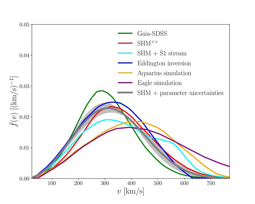
With the formalism developed in the previous section, it is possible to determine the deviation of the true dark matter velocity distribution to a given reference velocity distribution. Concretely, we calculate this for the velocity distributions extracted from the Aquarius and Eagle simulations [7, 51], determined using Eddington’s formula [14] and reconstructed from the motion of stars [11, 52, 13]. We confront each of those distributions to the Standard Halo Model, which models the velocity distribution as a Maxwell-Boltzmann distribution

$$f_{\text{SHM}}(\vec{v})=\frac{1}{N_{\text{esc}}\,(2\pi\,\sigma_{v}^{2})^{3/2}}\,\exp\left(-\frac{\vec{v}^{2}}{2\,\sigma_{v}^{2}}\right)\,,$$ (14)

where $\sigma_{v}\approx 156\,\text{km/s}$ is the velocity dispersion [53, 54]. The normalization constant $N_{\text{esc}}$ depends on the escape velocity $v_{\text{esc}}\approx 544\,\text{km/s}$ [55, 56] and is given by

$$N_{\text{esc}}=\text{erf}\left(\frac{v_{\text{esc}}}{\sqrt{2}\sigma_{v}}\right)-\sqrt{\frac{2}{\pi}}\,\frac{v_{\text{esc}}}{\sigma_{v}}\,\exp\left(-\frac{v_{\text{esc}}^{2}}{2\sigma_{v}^{2}}\right)\,.$$ (15)

In Tab. 2, we give the values of the distance of some velocity distributions to the SHM. In each case, we consider the angular averaged distributions in the solar rest frame

$$f_{0}(v)=v^{2}\,\int\text{d}\Omega_{v}\,f(\vec{v}+\vec{v}_{\odot})\,,$$ (16)

where $\vec{v}_{\odot}$ is the velocity of the Sun with respect to the Galactic rest fame. The velocity of the Sun is composed of the motion of the local standard of rest (LSR) and the peculiar motion of the Sun with respect to the LSR, i.e.

$$\vec{v}_{\odot}=\vec{v}_{\text{LSR}}+\vec{v}_{\odot,\text{pec}}\,.$$ (17)

Concretely, the motion of the LSR is given by $\vec{v}_{\text{LSR}}=(0,v_{c},0)$ where $v_{c}\approx 220\,\text{km/s}$ [53] is the local circular speed. Furthermore, the latest determination of the Sun’s peculiar motion finds $\vec{v}_{\odot,\text{pec}}=(11.1,12.24,7.25)\,\text{km/s}$ [57].

Figure 2: Left plot: A variety of dark matter velocity distributions discussed in the literature and obtained with different methods. Right plot: Optimized velocity distributions of a direct detection experiment, for a given dark matter mass and maximal distance that the true distribution can deviate from the Maxwell-Boltzmann. The colored regions represent the family of velocity distributions that deviate at most a value of $D_{KL}$=0.1 from the Maxwell-Boltzmann. It is clearly visible that the uncertainties in the dark matter velocity distribution can be very well parameterized with our method.

	$L^{1}$	$L^{2}$	$L^{\infty}$	$D_{\chi^{2}}$	$D_{KL}$
SHM parameter uncertainties	$\leq 0.101$	$\leq 0.024$	$\leq 0.004$	$\leq 1.822$	$\leq 0.040$
Eagle simulation [9]	0.258	0.057	0.0086	9.73	0.217
Aquarius simulation [7]	0.225	0.052	0.0083	0.730	0.144
Eddington inversion [14]	0.060	0.016	0.0034	0.030	0.018
SHM + S1 stream [13]	0.118	0.029	0.0064	0.223	0.050
SHM++ [12]	0.067	0.016	0.0032	0.096	0.019
Gaia-SDSS [11]	0.103	0.027	0.0064	0.060	0.037

Table 2: Deviations from SHM for different velocity distributions and distance measures. Concretely, we show the distance of the SHM to velocity distributions extracted from the Eagle simulation [9], from the Aquarius simulation [7], from Eddington’s result [14] and from local tracers of dark matter [13, 12, 11]. Furthermore, we show the distance implied by parametric uncertainties of the SHM.

As the parameters $\sigma_{v}$ and $v_{\text{esc}}$ describing the SHM are subject uncertainties of about 10%, we also show the deviations of SHM velocity distributions with parameters $v_{0}=\sqrt{2}\sigma_{v}$ within the range $[200,240]\,\text{km/s}$ and $v_{\text{esc}}$ within $[500,600]\,\text{km/s}$ to the SHM with the canonical values of $v_{0}=220\,\text{km/s}$ and $v_{\text{esc}}=544\,\text{km/s}$.
As apparent from the results presented in Tab. 2, the conclusions drawn from the comparison of different velocity distributions are independent of the distance. However, the scaling of every distance measure changes. Concretely, we find that velocity distributions extracted from the Aquarius and Eagle simulations [7, 51] and from local tracers of dark matter [11] deviate more from the SHM than justified by uncertainties of the SHM input parameters. Furthermore, we find that the velocity distribution determined in Ref. [14] using Eddington’s result deviates less from the canonical SHM than the deviations due to uncertainties of the SHM parameters. However, we note that this does not imply the velocity distribution from [14] is well fit by the SHM.

5 Upper limits from nuclear recoil searches

The knowledge of the magnitude of the distance to the Maxwell-Boltzmann for various velocity distributions can be used to quantify the impact of uncertainties on the results of direct dark matter searches. Concretely, we will derive upper limits from the CRESST-III, LUX-ZEPLIN and PICO-60 experiments [58, 59, 60] which aim to detect dark matter by counting the number of scattering events between dark matter particles and nuclei in a detector. The expected number of events can be calculated by multiplying the exposure of the experiment by the recoil rate $R$ that is given by [61]

$$R=\int_{0}^{\infty}\,\sum\limits_{i}\epsilon_{i}(E_{R})\,\frac{\text{d}R_{i}}{\text{d}E_{R}}\,\text{d}E_{R}\,.$$ (18)

The recoil spectrum of dark matter particles off the nuclear species $N_{i}$ is given by

$$\frac{\text{d}R_{i}}{dE_{R}}=\frac{\xi_{i}\;\rho_{\text{loc}}}{m_{\text{DM}}\;m_{N_{i}}}\int_{v^{\geq}v_{\text{min,i}}(E_{R})}\text{d}^{3}\vec{v}\,v\,f(\vec{v})\,\frac{\text{d}\sigma_{i}}{dE_{R}}(v,E_{R})\,,$$ (19)

where $\vec{v}$ is the velocity of the dark matter particle in the laboratory frame [52]. We use the software DDCalc to calculate the nuclear recoil rates in CRESST-III, PICO60 and LUX-ZEPLIN [62, 63]. The differential scattering cross section of a dark matter particle with a specific nucleus $N_{i}$ with mass $m_{N_{i}}$ and mass fraction $\xi_{i}$ inside the detector is denoted by $\text{d}\sigma_{i}/\text{d}E_{R}$. A dark matter particle must have a velocity larger than $v_{\text{min},i}(E_{R})=\sqrt{m_{N_{i}}E_{R}/(2\mu_{N_{i}}^{2})}$ in order to transfer energy $E_{R}$ onto the nucleus, where $\mu_{N_{i}}$ is the reduced mass of the dark matter-nucleus system. We model the dark matter velocity distribution as a superposition of streams [40]

$$f(\vec{v})=\sum\limits_{j}\,f(\vec{v}_{j})\,w_{j}\,\delta(\vec{v}-\vec{v}_{j}),$$ (20)

where $w_{i}$ are integration weights and $f(\vec{v}_{j})$ is the velocity distribution evaluated at the velocity $\vec{v}_{j}$. Defining $x_{j}\equiv f(\vec{v}_{j})\,w_{j}$, we can relate the numerical integration to a decomposition of the velocity distribution into streams. Applying this to the recoil rate at a direct detection experiment yields

$$R=\sum\limits_{j}R(\vec{v}_{j})\,x_{j}\,,$$ (21)

where $R(\vec{v}_{j})$ is the response of the detector to a stream of dark matter particles with velocity $\vec{v}_{j}$. This can be calculated from Eq. (18) by replacing the velocity distribution with a delta function

$$R(\vec{v}_{j})=\sum\limits_{i}\,\int_{0}^{\infty}\text{d}E_{R}\,\frac{\xi_{i}\;\rho_{\text{loc}}}{m_{\text{DM}}\;m_{N_{i}}}\Theta\left(v_{j}-v_{\text{min,i}}(E_{R})\right)\,v_{j}\,\frac{\text{d}\sigma_{i}}{dE_{R}}(v_{j},E_{R})\,.$$ (22)

This discretization allows us to apply the optimization techniques discussed in section 2. We aim to optimize the number of recoil events induced by dark matter in an experiment, subject to the constraint that the dark matter velocity distribution deviates at most a given value $\Delta$ from a Maxwell-Boltzmann distribution, that it is positively defined, and that all dark matter particles reaching the Earth are bound to the Galaxy. The optimization over a domain of velocities $\vec{v}_{0}$ reads:

$$\text{{Optimize:} }\mathcal{R}[f]=\int d^{3}vf(\vec{v}_{0})R_{\vec{v}_{0}}$$ (23)

subject to:

$$\int d^{3}v_{0}f(\vec{v}_{0})=1$$

$$D(f_{\rm MB},f)\leq\Delta$$

$$f(\vec{v}_{0})\geq 0$$

$$v_{0}\leq v_{\rm esc}$$

where the constraint $D(f,f_{\rm MB})\leq\Delta$ imposes that the maximal distance between the true dark matter distribution and the Maxwell-Boltzmann is given by $\Delta$, where the devitation is parametrized with a distance measure as those described in section 3. This problem can be formulated on general grounds, as we have done, but one needs to write it in its discretized form for each distance measure under consideration and check the convexity of the problem. In the following, we will focus on two norms ($L^{1}$ and $L^{\infty}$) and two information divergences (KL-divergence and $\chi^{2}$ divergence). These $L^{1}$-norm, $L^{\infty}$-norm and the $\chi^{2}$-divergence satisfy the convexity requirements of Problem 23 and can be recasted as Second Order Cone problems (SOCP’s), solvable by CVXPY, see [50] for further details. The KL-divergence can also be converted into a convex constraint by transforming it into a form in which it belongs to the exponential cone. The convex constraint would be given by $\Delta\geq D_{KL}(f_{\rm MB},f)$ and is equivalent to

$$\Delta\geq D(f_{\rm MB},f)\Longleftrightarrow-\Delta\leq f_{\rm MB}\log(f/f_{\rm MB})\Longleftrightarrow(f,f_{\rm MB},-\Delta)\in K_{\exp},$$ (24)

where the exponential cone $K_{\exp}$ is described in Appendix A. We would like to stress that in the literature the KL-divergence is typically used in convex optimization problems as the objective function, but not as a constraint of the optimization problem under consideration. Our methodology is perhaps not new but definitely not widespread, not only in this particular physics context but in generic convex optimization studies.

Figure 3: Upper and middle panels: 90% CL upper limits on the spin-independent dark matter-nucleon cross section from the CRESST-III experiment, for different deviations w.r.t the SHM. The coloured bands represent the set of upper limits obtained from those feasible velocity distributions that satisfy the experimental constraints and deviate at most a certain value with respect to the SHM. From upper left to lower right, we show the results obtained for the $L^{1}$-norm, $L^{\infty}$-norm, Neyman $\chi^{2}$-divergence and KL-divergence. For comparison, we show in colored dotted lines the limits derived for four different halo models. Lower panels: Constraints on the spin-independent dark matter-nucleon cross section from the LUX-ZEPLIN experiment, and on the spin-dependent dark matter-nucleon cross section from the PICO-60 experiment, for different deviations w.r.t the SHM parametrized by the KL-divergence.

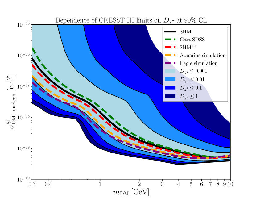
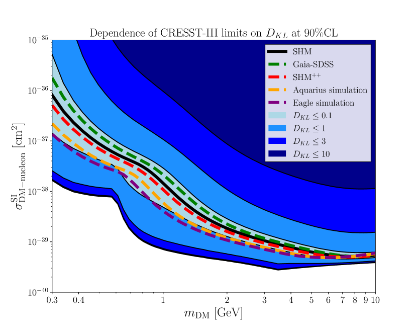
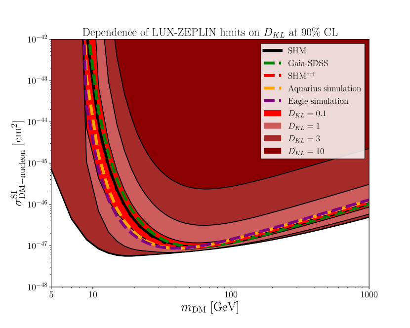
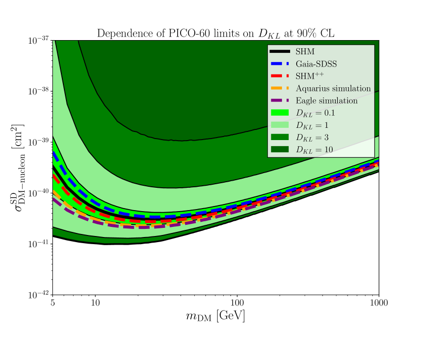
We can apply the developed methodology to derive upper limits in a direct detection experiment for different values of the distance measure parametrizing the deviation from the Maxwell-Boltzmann velocity distribution. In Fig. 3 we present optimized upper limits on the dark matter mass-cross section parameter space at $90\%$ C.L from the CRESST-III, LUX-ZEPLIN and PICO-60 experiments. In the following, we discuss and interpret the results in some detail.

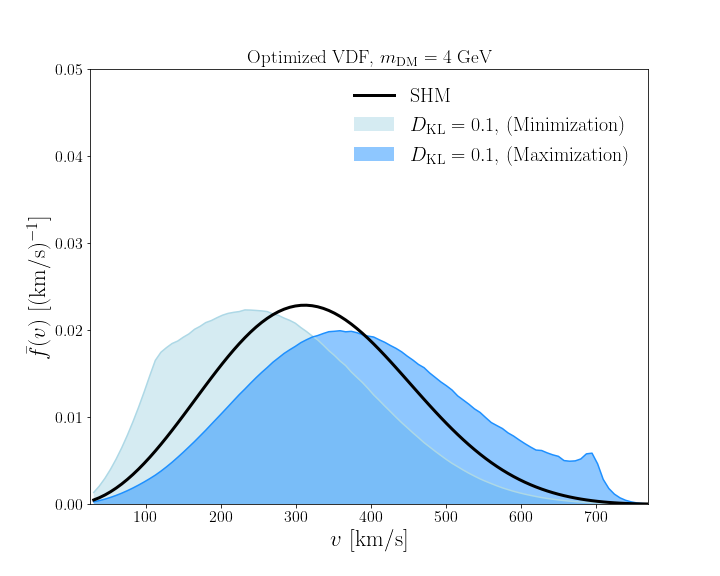
When solving the problem 23 maximizing the number of events, the optimized velocity distributions approach a single stream of dark matter particles moving at the Milky Way escape velocity, and all distance measures perform similarly. When minimizing, the discrepancy between different distances is not only due to the different scaling of each distance, but also due to the way in which the distance measure applies. At low masses, the $L^{1}$-norm behavior can be explained kinematically. As its magnitude increases, the high velocity tail is suppressed and, at a certain deviation, the experiment is not sensitive to such velocity distributions anymore. The $\chi^{2}$-divergence shows a similar behaviour as the $L^{1}$-norm, being the deviation at low masses ($m_{\rm DM}\sim$ 0.3 GeV) very large, and compensated at higher masses ($m_{\rm DM}\sim$ 10 GeV), where the experiment is kinematically sensitive to the complete velocity spectrum. Deviations are then washed out, since the $\chi^{2}$-divergence optimized velocity distributions resemble two pronounced peaks in both the low and high velocity tails, suppressing completely the Maxwell-Boltzmann most probable speed peak.

The $L^{\infty}$-norm and the KL-divergence perform quite differently. The $L^{\infty}$-norm parametrizes a larger impact of the velocity distribution at low masses, but the optimized velocity distributions do not lie completely below the velocity threshold of the experiment. They rather retain a fraction of the kinematically accessible spectrum, such that optimized upper limits do not deviate so sharply at low masses from the SHM one as it happens for other distance measures. This effect is even more pronounced in the case of the KL-divergence, which does not suppress the high velocity tail at low dark matter masses. This explains that the upper limits do not deviate so largely with respect to the SHM upper limit.

The KL-divergence parametrization suggests, against our kinematic intuition, that there could be feasible velocity distributions that cause an uncertainty in the results shown by a given experiment that is larger at high masses than at low masses. This can happen since the KL-divergence does not penalize the high velocity tail so strongly but smoothly interpolates between the Maxwell-Boltzmann-like velocity distribution and the most aggressive/conservative velocity distributions. For example, the CRESST experiment is sensitive to the complete dark matter velocity spectrum at 10 GeV, hence, differences between the distributions at low masses are taken into account. For sufficiently low masses ($m_{\rm DM}\leq 1$ GeV), only the high velocity tail is seen and there the KL does not penalize it so strongly, therefore being the difference in the upper limits not so large. We notice that the inequality Ref. 12 holds for our analysis. Indeed, the $L^{\infty}$-norm scaling is significantly lower than the KL-divergence, obtaining similar deviations for values of $L^{\infty}$= 0.001 and $D_{KL}$ = 0.1. We have, as well, shown the upper limits for four specific halo models: from the Aquarius and Eagle simulations, and the SHM⁺⁺ and Gaia-SDSS combined data velocity distributions. We notice that for each distance measure, even though the deviation is not so strong, $\mathcal{O}(1)$, these fall in different bands, which motivates the need of using different distance measures to make a proper halo-independent analysis. As we have already mentioned, in Tab. 2, we have computed the distance measure between different halo models and the Maxwell-Boltzmann velocity distribution, in order to get a hint of which deviations of our analysis are consistent with experimental results and are physically motivated. We notice that, in the case of tracers studies, we obtain deviations in the two closest bands to the SHM upper limit, leading in some regions to uncertainties of $\mathcal{O}(10)$. For the case of N-body simulations, these uncertainties can reach values of $\mathcal{O}(10^{2})$ in some regions of the parameter space. These of course depend on the distance measure under consideration and we remark that for the KL-divergence we do not encounter physically motivated deviations larger than $\mathcal{O}(1)$.

6 Upper limits from electron recoil searches

We can also interpret the results of dark matter-electron scattering searches using the method presented in sections 2 and 3. The results may vary w.r.t the nuclear recoil case due to different kinematics (the recoiling electron is bound without fixed momentum), and different energy threshold from experiments. In liquid xenon, for a given stream velocity $\vec{v}$ in the galactic frame with modulus $v$, the differential ionization cross section reads [64]

$$\frac{d\sigma_{ion}^{nl}}{d\text{ln}E_{er}}(v,E_{er})=\frac{\bar{\sigma}_{e}}{8\mu_{e}^{2}v^{2}}\int_{q^{nl}_{\rm min}}^{q^{nl}_{\rm max}}dqq\left|f_{ion}^{nl}(k^{\prime},q)\right|^{2}\left|F_{\mathrm{DM}}(q)\right|^{2}.$$ (25)

where the minimum and maximum momentum transfer in the orbital $(n,l)$ is given by

$$q^{nl}_{\begin{subarray}{c}{\rm max}\\ {\rm min}\end{subarray}}(E_{er})=m_{\rm DM}v\pm\sqrt{m_{\rm DM}^{2}v^{2}-2m_{\rm DM}(E_{er}+\left|E^{n,l}\right|)}$$ (26)

and the differential ionization rate is

$$\frac{dR_{ion}^{\vec{v}}}{d\text{ln}E_{er}}=N_{T}\frac{\rho_{\rm DM}}{m_{\rm DM}}\frac{1}{v}\,\sum_{n,l}\frac{\text{d}\sigma_{\rm ion}^{nl}}{d\text{ln}E_{er}}(v,E_{er})\,,$$ (27)

Here, $\mu_{\rm DM,e}$ is the reduced mass of the dark matter-electron system, $\bar{\sigma}_{\rm DM-e}$ is the dark matter-free electron scattering cross section at fixed momentum transfer $q=\alpha m_{e}$, $\left|f_{ion}^{nl}(k^{\prime},q)\right|^{2}$ is the ionization form factor of an electron in the $(n,l)$ shell with final momentum $k^{\prime}=\sqrt{2m_{e}E_{er}}$ and momentum transfer $q$, and $F_{\mathrm{DM}}(q)$ is a form factor that encodes the $q$-dependence of the squared matrix element for dark matter-electron scattering and depends of the mediator under consideration. Finally, the total number of expected ionization events for a given stream reads ${\cal N}=R_{ion}\cdot\mathcal{E}$, with $R_{ion}$ the total ionization rate, calculated from integrating Eq.(27) over all possible recoil energies, and $\mathcal{E}$ the exposure (i.e. mass multiplied by live-time) of the experiment. In our analysis, we consider the ionization of electrons in the following orbitals (with binding energies in eV shown in parenthesis: $5p^{6}$ (12.4), $5s^{2}$ (25.7), $4d^{10}$ (75.6), $4p^{6}$ (163.5) and $3s^{2}$ (1148.7). The corresponding ionization form factors were obtained from the software QEDark [65]. For the dark matter form factor, we adopt three different parametrizations: the case of a heavy hidden photon $A^{\prime}$ mediator $m_{A^{\prime}}\gg q$, with $F_{\mathrm{DM}}(q)$=1, an interaction via an electric dipole moment $F_{\mathrm{DM}}(q)=\alpha m_{e}/q$, and an interaction via an ultralight or massless hidden photon $m_{A^{\prime}}\ll q$, with $F_{\mathrm{DM}}(q)=\alpha^{2}m_{e}^{2}/q^{2}$.

For semiconductor detectors, the dark matter-electron scattering rate for a given stream velocity v is given by [66, 67]

$$R_{ion}^{\vec{v}}=\frac{1}{\rho_{T}}\frac{\rho_{\rm DM}}{m_{\rm DM}}\frac{\bar{\sigma}_{e}}{\mu_{e}^{2}}\frac{\pi}{\alpha}\int\frac{d^{3}\mathbf{k}}{(2\pi)^{3}}k^{2}\left|F_{\rm DM}(k)\right|^{2}\int\frac{d\omega}{2\pi}\frac{1}{1-e^{-\beta\omega}}\operatorname{Im}\left[\frac{-1}{\epsilon(\omega,\mathbf{k})}\right]\delta\left(\omega+\frac{k^{2}}{2m_{\chi}}-\mathbf{k}\cdot\mathbf{v}\right)$$ (28)

where $w$ is the energy deposited in the material, $\vec{q}$ is the momentum transfer of the process, and $\rho_{T}$ is the target density. The rate involves an integration of the Electronic Loss Function (ELF) of the target material, which we calculate with DarkELF [67]. For the dielectric function $\epsilon(\omega,\mathbf{k})$, we use the Lindhard method, which treats the target as a non-interacting Fermi liquid.

In order to calculate the rate for an arbitrary velocity distribution, it is simply necessary to calculate

$$R_{ion}=\sum_{i}a_{\vec{v}_{i}}R_{ion}^{\vec{v}_{i}}$$ (29)

where $a_{i}$ is the discrete probability of having a dark matter particle moving with velocity $\vec{v_{i}}$.

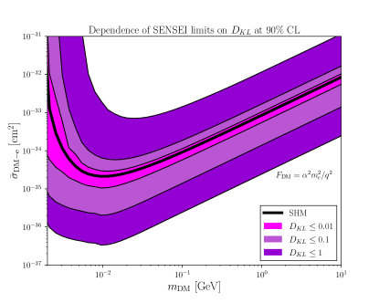
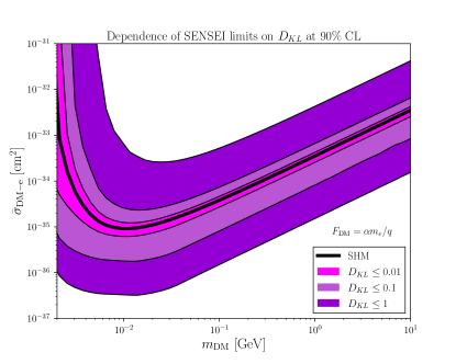
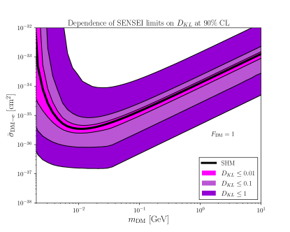
We want to derive 90$\%$ C.L upper limits on the dark matter-electron cross section from SENSEI, when varying the dark matter flux, and given a maximal deviation from the flux determined by the SHM. In this case, unlike we did in our analysis for nuclear recoils in section 5, we will allow for the possibility that a component of dark matter particles with velocities larger than the escape velocity of the Milky Way reaches the Earth. Thus, we solve the following optimization problem

Optimize:

$$\sum_{i}a_{\vec{v}_{i}}R_{ion}^{\vec{v}_{i}}$$ (30)

subject to:

$$D_{\rm KL}(f_{\rm MB},f)\leq\Delta$$

$$\sum_{i=1}a_{\vec{v}_{i}}=1$$

$$a_{\vec{v}_{i}}\geq 0$$

and the results are shown in Figure 4. We find similar conclusions as for dark matter-nucleon scatterings, although with two main differences. The uncertainties are somewhat larger at low masses, extending over 2 to 3 orders of magnitude for $D_{\rm KL}\leq 1$, and the uncertainties on the velocity distribution manifest more strongly at high dark matter masses than for nuclear recoils, since the electron momentums in the orbital is not fixed. This aspect was discussed previously in [17].

Figure 4: Upper limits at 90$\%$ CL from SENSEI, for different maximal deviations (parametrized by the KL divergence) from the Maxwell Boltzmann velocity distribution, and a maximal dark matter velocity of 0.1c.

We also entertain the possibility to use these methods to confront a future signal in a given dark matter-electron scattering experiment with a null signal from a given experiment. We solve in this case the same optimization problem as described previously, but introducing an additional constraint ensuring that the optimized velocity distribution still gives a null result in one of the experiments. Concretely,

Maximize:

$$\sum_{i}a_{\vec{v}_{i}}R_{ion,\rm XENON1T}^{\vec{v}_{i}}$$ (31)

subject to:

$$D_{\rm KL}(f_{\rm MB},f)\leq\Delta$$

$$\sum_{i=1}a_{\vec{v}_{i}}=1$$

$$a_{\vec{v}_{i}}\geq 0$$

$$\sum_{i}a_{\vec{v}_{i}}R_{ion,\rm SENSEI}^{\vec{v}_{i}}$$

In Figure 5 we show the maximum number of events that can be obtained in XENON1T, assuming an energy threshold from its S2-only analysis data [68], which is 0.18 keV, and assuming the null results from SENSEI with a projected exposure 10 times larger than the current one, which is 48 days $\times$ grams. We do this exercise for different values of the dark matter mass, interaction model and maximum deviation from the Maxwell-Boltzmann. In this way we show that a future signal might be confronted with a null result independently from the assumptions on the halo model, just fixing the maximal deviation from the SHM in a sounded statistical manner.

Figure 5: Hypothetical optimized number of events in XENON1T, subject to the null results of SENSEI experiment with 10 times more exposure than currently, and from varying the DM velocity distribution w.r.t to the Maxwell-Boltzmann in a model independent manner. For comparison, we show in magenta a hypothetical number of signal events observed in XENON1T.

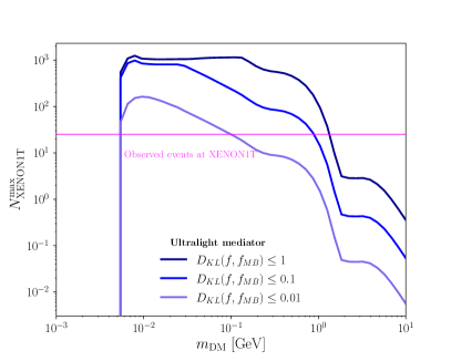
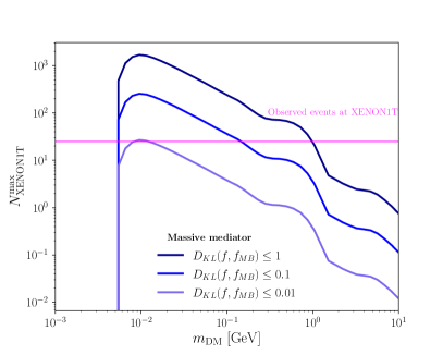
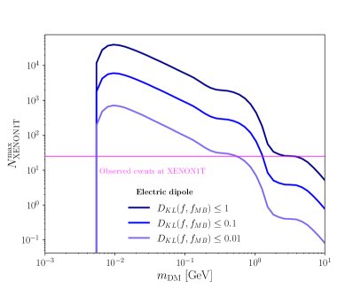
As can be seen in the plot, the complementarity of XENON1T and SENSEI is clearly more apparent at high dark matter masses, and the ultralight mediator or dipole model shows more complementarity between experiments, since SENSEI threshold to low energy depositions enhances its sensitivity to these models. On the contrary, for a massive mediator, XENON1T sensivity supersedes SENSEI by orders of magnitude, thus, it is more likely than a signal in XENON1T will be observed in SENSEI as well. Indeed, as can be seen in the plot, for values of the KL-divergence below 0.01, a signal would be incompatible with a null result, even with current SENSEI exposures. We also point out that in our figures, the lowest dark matter mass probed is set by the maximal dark matter velocity considered in the optimization problem (0.1 c).

In this discussion, we have not addressed the potential overlap of a direct dark matter-electron signal with an ionization signal from the Migdal effect due to light dark matter-nucleus scatterings [69, 70, 71]. The Migdal effect signal is expected to be subdominant at the XENON1T, but may become larger to the dark matter-electron scattering signal at the energies probed by SENSEI. Moreover, in the future the sensitivity of these experiments may reach the ionization signal induced by neutrino-nucleus or neutrino-electron scattering [69, 72, 73, 64, 74], and the "number of events" counting analysis done here would be incomplete. A more refined analysis accounting for spectral features would become needed. Our convex-opimitizaion technique could be adapted to more sophisticated likelihood analysis.

7 Conclusions

We have discussed a method to bracket the uncertainty in the theoretical prediction of an observable functional $\mathcal{F}[f]$, consisting in in using methods of convex optimization to sample over all functions $f$ lying within a given distance measure from a central function. In this manner, we account for the uncertainties in the functional $\mathcal{F}[f]$, without assuming any parametric form of the function $f$, as it is typically done in the high-energy physics literature. Our discussion is focused on constraints consisting on distance measures $D(f,f_{0})$ between a reference function $f_{0}$ and the optimized function $f$, given by information divergences.

We applied this method to quantify the impact of the uncertainties in the dark matter velocity distribution in direct detection experiments with information divergences. By using this technique, we have derived upper limits on the spin-independent (spin-dependent) dark matter scattering cross section using CRESST-III and LUX-ZEPLIN (PICO-60) data, accounting for uncertainties in the velocity distribution with different distance measures. We find $\mathcal{O}(1-10)$ uncertainties in direct detection experiments upper limits, for values of the distance measures compatible with dark matter velocity distributions obtained from simulations and observations. We have also derived limits on the dark matter electron-scattering cross section from SENSEI with this technique, sampling over a velocity range extending beyond the escape velocity of the Milky Way. We find uncertainties that are larger than for nuclear recoils, reaching values as high as 3 orders of magnitude, and extending towards larger masses. Finally, we have also explored the potential complementarity of XENON1T and SENSEI in probing a signal vs a null result in the future for different dark matter-electron interaction models. We find a strong complementarity at high masses, while at low masses the experiments are expected to become more degenerate to the dark matter velocity distribution, especially if the mediator of the interaction is ultralight or massless.

Furthermore, we have found that the KL-divergence is a statistically more robust way to account for dark matter astrophysical uncertainties than the relative differences used in [39], since it is less constrained by initial assumptions on the shape of the distribution, and the feasible set of velocity distributions that respect this constraint is more varied than for other distance measures. The presence of the logarithm in the KL-divergence causes the optimized velocity distributions to have smoother shapes, that could match physically motivated velocity distributions like those obtained from simulations and observations. However, we emphasize that this methodology does not reconstruct the dark matter velocity distribution from the experimental data, but rather are mathematically optimized distributions that allow for an interpolated model-independent analysis.

The parametrization of the uncertainties of a function with information divergences allows to account for uncertainties in physical observables in a novel manner. In some scenarios, a parametric form for the physical function $f$ might be well motivated, and accounting for its uncertainties by varying the value of its parameters could be already be a robust approach. On the other hand, in many other scenarios the true parametric form of the function $f$ could strongly differ from the theoretical prior, and the interpretation of experimental results on the observable $\mathcal{F}[f]$ could be inadequate, given the wrong parametric estimate of $f$. We hope that the techniques present in this work could help a more robust interpretation of experimental results in high-energy and astroparticle physics, particularly in dark matter direct detection searches.

Acknowledgments

We are very grateful to Alejandro Ibarra for supervision of part of this project during the Master and PhD theses of GH and AR, and for providing insightful feedback on this method, particularly on its potential application to other physical scenarios beyond direct detection. We are also grateful to Anja Brenner, Stefano Scopel and Gaurav Tomar for useful discussions. GH is grateful to the members of the CRESST collaboration for useful conversations and feedback on direct detection experiments during his Master Thesis, and to Felix Kahlhöfer for help on learning and using the software DDCalc. This work is supported by the Collaborative Research Center SFB1258, and by the Deutsche Forschungsgemeinschaft (DFG, German Research Foundation) under Germany’s Excellence Strategy - EXC-2094 - 390783311. The work of GH is also supported by the U.S. Department of Energy Office of Science under award number DE-SC0020262

Appendix A Exponential cone problems

Many optimization problems can contain exponentials and logarithms. These can sometimes be modelled with the exponential cone, which is a convex subset of $\mathbb{R}^{3}$ defined as [75]

$$K_{\exp}=\left\{\left(x_{1},x_{2},x_{3}\right):x_{1}\geq x_{2}e^{x_{3}/x_{2}},x_{2}>0\right\}\cup\\ \left\{\left(x_{1},0,x_{3}\right):x_{1}\geq 0,x_{3}\leq 0\right\}$$ (32)

Thus the exponential cone is the closure in $\mathbb{R}^{3}$ of the set of points which satisfy

$$x_{1}\geq x_{2}e^{x_{3}/x_{2}},x_{1},x_{2}>0$$ (33)

When working with logarithms, as in the case of the KL-divergence, Eq. 33 can be rewritten as

$$x_{3}\leq x_{2}\log\left(x_{1}/x_{2}\right),x_{1},x_{2}>0$$ (34)

Alternatively, it can be written as

$$x_{1}/x_{2}\geq e^{x_{3}/x_{2}},x_{1},x_{2}>0$$ (35)

This shows that $K_{exp}$ is a cone, i.e. $\alpha x\in K_{exp}$ for $x\in K_{exp}$ and $\alpha\geq 0$. The convexity of $K_{exp}$ follows from the fact that the Hessian of $f(x,y)=y\exp(x/y)$,

$$D^{2}(f)=e^{x/y}\left[\begin{array}[]{cc}y^{-1}&-xy^{-2}\\ -xy^{-2}&x^{2}y^{-3}\end{array}\right]$$

is positive semidefinite for $y>0$.

References

- [1] S. Kullback and R.. Leibler “On Information and Sufficiency” In Ann. Math. Statist. 22.1 The Institute of Mathematical Statistics, 1951, pp. 79–86 DOI: 10.1214/aoms/1177729694
- [2] Alfréd Rényi “On Measures of Entropy and Information”, 1961 URL: https://api.semanticscholar.org/CorpusID:123056571
- [3] Imre Csiszár “Eine informationstheoretische ungleichung und ihre anwendung auf beweis der ergodizitaet von markoffschen ketten” In Magyer Tud. Akad. Mat. Kutato Int. Koezl. 8, 1964, pp. 85–108
- [4] Stephen Boyd and Lieven Vandenberghe “Convex Optimization” Cambridge University Press, 2004 DOI: 10.1017/CBO9780511804441
- [5] Steven Diamond and Stephen Boyd “CVXPY: A Python-embedded modeling language for convex optimization” In Journal of Machine Learning Research 17.83, 2016, pp. 1–5
- [6] Michael Grant, Stephen Boyd and Yinyu Ye “Disciplined convex programming” In Global Optimization: From Theory to Implementation, Nonconvex Optimization and Its Application Series Springer, 2006, pp. 155–210
- [7] Mark Vogelsberger et al. “Phase-space structure in the local dark matter distribution and its signature in direct detection experiments” In Mon. Not. Roy. Astron. Soc. 395, 2009, pp. 797–811 DOI: 10.1111/j.1365-2966.2009.14630.x
- [8] A.. Baushev “Extragalactic dark matter and direct detection experiments” In Astrophys. J. 771, 2013, pp. 117 DOI: 10.1088/0004-637X/771/2/117
- [9] Joop Schaye et al. “The EAGLE project: simulating the evolution and assembly of galaxies and their environments” In Monthly Notices of the Royal Astronomical Society 446.1 Oxford University Press (OUP), 2014, pp. 521–554 DOI: 10.1093/mnras/stu2058
- [10] Anne M Green “Astrophysical uncertainties on the local dark matter distribution and direct detection experiments” In J. Phys. G 44.8, 2017, pp. 084001 DOI: 10.1088/1361-6471/aa7819
- [11] Lina Necib, Mariangela Lisanti and Vasily Belokurov “Dark Matter in Disequilibrium: The Local Velocity Distribution from SDSS-Gaia”, 2018 arXiv:1807.02519 [astro-ph.GA]
- [12] N. Evans, Ciaran A.. O’Hare and Christopher McCabe “SHM++: A Refinement of the Standard Halo Model for Dark Matter Searches in Light of the Gaia Sausage”, 2018 arXiv:1810.11468 [astro-ph.GA]
- [13] Ciaran A.. O’Hare et al. “Dark matter hurricane: Measuring the S1 stream with dark matter detectors” In Physical Review D 98.10 American Physical Society (APS), 2018 DOI: 10.1103/physrevd.98.103006
- [14] Sayan Mandal, Subhabrata Majumdar, Vikram Rentala and Ritoban Basu Thakur “Observationally inferred dark matter phase-space distribution and direct detection experiments” In Phys. Rev. D100.2, 2019, pp. 023002 DOI: 10.1103/PhysRevD.100.023002
- [15] Gurtina Besla, Annika Peter and Nicolas Garavito-Camargo “The highest-speed local dark matter particles come from the Large Magellanic Cloud” In JCAP 11, 2019, pp. 013 DOI: 10.1088/1475-7516/2019/11/013
- [16] Jatan Buch, JiJi Fan and John Shing Chau Leung “Implications of the Gaia Sausage for Dark Matter Nuclear Interactions” In Phys. Rev. D 101.6, 2020, pp. 063026 DOI: 10.1103/PhysRevD.101.063026
- [17] Gonzalo Herrera and Alejandro Ibarra “Direct detection of non-galactic light dark matter” In Phys. Lett. B 820, 2021, pp. 136551 DOI: 10.1016/j.physletb.2021.136551
- [18] Gonzalo Herrera, Alejandro Ibarra and Satoshi Shirai “Enhanced prospects for direct detection of inelastic dark matter from a non-galactic diffuse component” In JCAP 04, 2023, pp. 026 DOI: 10.1088/1475-7516/2023/04/026
- [19] Adam Smith-Orlik “The impact of the Large Magellanic Cloud on dark matter direct detection signals”, 2023 arXiv:2302.04281 [astro-ph.GA]
- [20] Andrzej Hryczuk, Ekaterina Karukes, Leszek Roszkowski and Matthew Talia “Impact of uncertainties in the halo velocity profile on direct detection of sub-GeV dark matter”, 2020 DOI: 10.1007/JHEP07(2020)081
- [21] Jatan Buch, Manuel A. Buen-Abad, Jiji Fan and John Shing Chau Leung “Dark Matter Substructure under the Electron Scattering Lamppost” In Phys. Rev. D 102.8, 2020, pp. 083010 DOI: 10.1103/PhysRevD.102.083010
- [22] Tarak Nath Maity, Tirtha Sankar Ray and Sambo Sarkar “Halo uncertainties in electron recoil events at direct detection experiments” In Eur. Phys. J. C 81.11, 2021, pp. 1005 DOI: 10.1140/epjc/s10052-021-09805-2
- [23] Aria Radick, Anna-Maria Taki and Tien-Tien Yu “Dependence of Dark Matter - Electron Scattering on the Galactic Dark Matter Velocity Distribution” In JCAP 02, 2021, pp. 004 DOI: 10.1088/1475-7516/2021/02/004
- [24] Tarak Nath Maity and Ranjan Laha “Dark matter substructures affect dark matter-electron scattering in direct detection experiments”, 2022 arXiv:2208.14471 [hep-ph]
- [25] Zheng-Liang Liang, Liangliang Su, Lei Wu and Bin Zhu “Plasmon-enhanced Direct Detection of sub-MeV Dark Matter”, 2024 arXiv:2401.11971 [hep-ph]
- [26] Rouven Essig, Ryan Plestid and Aman Singal “Collective excitations and low-energy ionization signatures of relativistic particles in silicon detectors”, 2024 arXiv:2403.00123 [hep-ph]
- [27] Patrick J. Fox, Jia Liu and Neal Weiner “Integrating Out Astrophysical Uncertainties” In Phys. Rev. D 83, 2011, pp. 103514 DOI: 10.1103/PhysRevD.83.103514
- [28] Patrick J. Fox, Graham D. Kribs and Tim M.. Tait “Interpreting Dark Matter Direct Detection Independently of the Local Velocity and Density Distribution” In Phys. Rev. D 83, 2011, pp. 034007 DOI: 10.1103/PhysRevD.83.034007
- [29] Paolo Gondolo and Graciela B. Gelmini “Halo independent comparison of direct dark matter detection data” In JCAP 12, 2012, pp. 015 DOI: 10.1088/1475-7516/2012/12/015
- [30] Juan Herrero-Garcia, Thomas Schwetz and Jure Zupan “Astrophysics independent bounds on the annual modulation of dark matter signals” In Phys. Rev. Lett. 109, 2012, pp. 141301 DOI: 10.1103/PhysRevLett.109.141301
- [31] Eugenio Del Nobile, Graciela B. Gelmini, Paolo Gondolo and Ji-Haeng Huh “Halo-independent analysis of direct detection data for light WIMPs” In JCAP 10, 2013, pp. 026 DOI: 10.1088/1475-7516/2013/10/026
- [32] Mads T. Frandsen et al. “The unbearable lightness of being: CDMS versus XENON” In JCAP 07, 2013, pp. 023 DOI: 10.1088/1475-7516/2013/07/023
- [33] Nassim Bozorgnia and Thomas Schwetz “What is the probability that direct detection experiments have observed Dark Matter?” In JCAP 12, 2014, pp. 015 DOI: 10.1088/1475-7516/2014/12/015
- [34] Brian Feldstein and Felix Kahlhoefer “A new halo-independent approach to dark matter direct detection analysis” In JCAP 08, 2014, pp. 065 DOI: 10.1088/1475-7516/2014/08/065
- [35] Mattias Blennow, Juan Herrero-Garcia and Thomas Schwetz “A halo-independent lower bound on the dark matter capture rate in the Sun from a direct detection signal” In JCAP 05, 2015, pp. 036 DOI: 10.1088/1475-7516/2015/05/036
- [36] Adam J. Anderson, Patrick J. Fox, Yonatan Kahn and Matthew McCullough “Halo-Independent Direct Detection Analyses Without Mass Assumptions” In JCAP 10, 2015, pp. 012 DOI: 10.1088/1475-7516/2015/10/012
- [37] Graciela B. Gelmini, Ji-Haeng Huh and Samuel J. Witte “Assessing Compatibility of Direct Detection Data: Halo-Independent Global Likelihood Analyses” In JCAP 10, 2016, pp. 029 DOI: 10.1088/1475-7516/2016/10/029
- [38] Felix Kahlhoefer and Sebastian Wild “Studying generalised dark matter interactions with extended halo-independent methods” In JCAP 10, 2016, pp. 032 DOI: 10.1088/1475-7516/2016/10/032
- [39] Alejandro Ibarra, Bradley J. Kavanagh and Andreas Rappelt “Bracketing the impact of astrophysical uncertainties on local dark matter searches” In JCAP 1812.12, 2018, pp. 018 DOI: 10.1088/1475-7516/2018/12/018
- [40] Alejandro Ibarra and Andreas Rappelt “Optimized velocity distributions for direct dark matter detection” In JCAP 08, 2017, pp. 039 DOI: 10.1088/1475-7516/2017/08/039
- [41] Riccardo Catena, Alejandro Ibarra, Andreas Rappelt and Sebastian Wild “Halo-independent comparison of direct detection experiments in the effective theory of dark matter-nucleon interactions” In JCAP 1807.07, 2018, pp. 028 DOI: 10.1088/1475-7516/2018/07/028
- [42] Andrew Fowlie “Non-parametric uncertainties in the dark matter velocity distribution” In Journal of Cosmology and Astroparticle Physics 2019.01 IOP Publishing, 2019, pp. 006–006 DOI: 10.1088/1475-7516/2019/01/006
- [43] Muping Chen, Graciela B. Gelmini and Volodymyr Takhistov “Halo-Independent Analysis of Direct Dark Matter Detection Through Electron Scattering”, 2021 arXiv:2105.08101 [hep-ph]
- [44] Muping Chen, Graciela B. Gelmini and Volodymyr Takhistov “Halo-Independent Dark Matter Electron Scattering Analysis with In-Medium Effects”, 2022 arXiv:2209.10902 [hep-ph]
- [45] Sunghyun Kang, Arpan Kar and Stefano Scopel “Halo-independent bounds on the non-relativistic effective theory of WIMP-nucleon scattering from direct detection and neutrino observations” In JCAP 03, 2023, pp. 011 DOI: 10.1088/1475-7516/2023/03/011
- [46] Sunghyun Kang, Arpan Kar and Stefano Scopel “Halo-independent bounds on Inelastic Dark Matter” In JCAP 11, 2023, pp. 077 DOI: 10.1088/1475-7516/2023/11/077
- [47] Elias Bernreuther et al. “Extracting Halo Independent Information from Dark Matter Electron Scattering Data”, 2023 arXiv:2311.04957 [hep-ph]
- [48] Benjamin Lillard “Wavelet-Harmonic Integration Methods”, 2023 arXiv:2310.01483 [hep-ph]
- [49] Benjamin Lillard “Vector Space Integration for Dark Matter Scattering”, 2023 arXiv:2310.01480 [hep-ph]
- [50] Andreas Günter Rappelt “Astrophysical uncertainties of direct dark matter searches”, 2020
- [51] Nassim Bozorgnia et al. “Simulated Milky Way analogues: implications for dark matter direct searches” In JCAP 05, 2016, pp. 024 DOI: 10.1088/1475-7516/2016/05/024
- [52] Christopher McCabe “The Earth’s velocity for direct detection experiments” In JCAP 1402, 2014, pp. 027 DOI: 10.1088/1475-7516/2014/02/027
- [53] F.. Kerr and Donald Lynden-Bell “Review of galactic constants” In Mon. Not. Roy. Astron. Soc. 221, 1986, pp. 1023
- [54] Anne M. Green “Astrophysical uncertainties on direct detection experiments” In Mod. Phys. Lett. A27, 2012, pp. 1230004 DOI: 10.1142/S0217732312300042
- [55] Martin C. Smith “The RAVE Survey: Constraining the Local Galactic Escape Speed” In Mon. Not. Roy. Astron. Soc. 379, 2007, pp. 755–772 DOI: 10.1111/j.1365-2966.2007.11964.x
- [56] Til Piffl “The RAVE survey: the Galactic escape speed and the mass of the Milky Way” In Astron. Astrophys. 562, 2014, pp. A91 DOI: 10.1051/0004-6361/201322531
- [57] Ralph Schönrich, James Binney and Walter Dehnen “Local kinematics and the local standard of rest” In Monthly Notices of the Royal Astronomical Society 403.4, 2010, pp. 1829–1833 DOI: 10.1111/j.1365-2966.2010.16253.x
- [58] A.. Abdelhameed “First results from the CRESST-III low-mass dark matter program” In Phys. Rev. D 100.10, 2019, pp. 102002 DOI: 10.1103/PhysRevD.100.102002
- [59] J. Aalbers “First Dark Matter Search Results from the LUX-ZEPLIN (LZ) Experiment”, 2022 arXiv:2207.03764 [hep-ex]
- [60] C. Amole “Dark Matter Search Results from the Complete Exposure of the PICO-60 C3F8 Bubble Chamber” In Phys. Rev. D 100.2, 2019, pp. 022001 DOI: 10.1103/PhysRevD.100.022001
- [61] David G. Cerdeno and Anne M. Green “Direct detection of WIMPs”, 2010 arXiv:1002.1912 [astro-ph.CO]
- [62] Torsten Bringmann “DarkBit: A GAMBIT module for computing dark matter observables and likelihoods” In Eur. Phys. J. C 77.12, 2017, pp. 831 DOI: 10.1140/epjc/s10052-017-5155-4
- [63] Peter Athron “Global analyses of Higgs portal singlet dark matter models using GAMBIT” In Eur. Phys. J. C 79.1, 2019, pp. 38 DOI: 10.1140/epjc/s10052-018-6513-6
- [64] Rouven Essig, Jeremy Mardon and Tomer Volansky “Direct Detection of Sub-GeV Dark Matter” In Phys. Rev. D 85, 2012, pp. 076007 DOI: 10.1103/PhysRevD.85.076007
- [65] Rouven Essig et al. “Direct Detection of sub-GeV Dark Matter with Semiconductor Targets” In JHEP 05, 2016, pp. 046 DOI: 10.1007/JHEP05(2016)046
- [66] Simon Knapen, Jonathan Kozaczuk and Tongyan Lin “Dark matter-electron scattering in dielectrics” In Phys. Rev. D 104.1, 2021, pp. 015031 DOI: 10.1103/PhysRevD.104.015031
- [67] Simon Knapen, Jonathan Kozaczuk and Tongyan Lin “python package for dark matter scattering in dielectric targets” In Physical Review D 105.1 American Physical Society (APS), 2022 DOI: 10.1103/physrevd.105.015014
- [68] E. Aprile “Light Dark Matter Search with Ionization Signals in XENON1T” In Phys. Rev. Lett. 123.25, 2019, pp. 251801 DOI: 10.1103/PhysRevLett.123.251801
- [69] Masahiro Ibe, Wakutaka Nakano, Yutaro Shoji and Kazumine Suzuki “Migdal Effect in Dark Matter Direct Detection Experiments” In JHEP 03, 2018, pp. 194 DOI: 10.1007/JHEP03(2018)194
- [70] Matthew J. Dolan, Felix Kahlhoefer and Christopher McCabe “Directly detecting sub-GeV dark matter with electrons from nuclear scattering” In Phys. Rev. Lett. 121.10, 2018, pp. 101801 DOI: 10.1103/PhysRevLett.121.101801
- [71] Rouven Essig, Josef Pradler, Mukul Sholapurkar and Tien-Tien Yu “Relation between the Migdal Effect and Dark Matter-Electron Scattering in Isolated Atoms and Semiconductors” In Phys. Rev. Lett. 124.2, 2020, pp. 021801 DOI: 10.1103/PhysRevLett.124.021801
- [72] Nicole F. Bell et al. “Migdal effect and photon bremsstrahlung in effective field theories of dark matter direct detection and coherent elastic neutrino-nucleus scattering” In Phys. Rev. D 101.1, 2020, pp. 015012 DOI: 10.1103/PhysRevD.101.015012
- [73] Gonzalo Herrera “A neutrino floor for the Migdal effect”, 2023 arXiv:2311.17719 [hep-ph]
- [74] Ben Carew, Ashlee R. Caddell, Tarak Nath Maity and Ciaran A.. O’Hare “The neutrino fog for dark matter-electron scattering experiments”, 2023 arXiv:2312.04303 [hep-ph]
- [75] MOSEK ApS “The MOSEK optimization toolbox for MATLAB manual. Version 9.0.”, 2019 URL: http://docs.mosek.com/9.0/toolbox/index.html