Reappraisal of SU(3)-flavor breaking in $B\rightarrow DP$

Abstract

In light of recently found deviations of the experimental data from predictions from QCD factorization for $B_{(s)}\rightarrow D_{(s)}P$ decays, where $P=\{\pi,K\}$, we systematically probe the current status of the SU(3)_F expansion from a fit to experimental branching ratio data without any further theory input. We find that the current data is in agreement with the power-counting of the SU(3)_F expansion. While the SU(3)_F limit is excluded at $>5\sigma$, SU(3)_F-breaking contributions of $\sim 20\%$ suffice for an excellent description of the data. SU(3)_F breaking is needed in tree ($>5\sigma$) and color-suppressed tree ($2.4\sigma$) diagrams. We are not yet sensitive to SU(3)_F breaking in exchange diagrams. From the underlying SU(3)_F parametrization we predict the unmeasured branching ratios $\mathcal{B}(\overline{B}_{s}^{0}\rightarrow\pi^{-}D^{+})=2\mathcal{B}(\overline{B}_{s}^{0}\rightarrow\pi^{0}D^{0})=[0.3,7.2]\times 10^{-6}$ of suppressed decays that can be searched for at the LHCb Upgrade I and LHCb Upgrade II experiments respectively.

I Introduction

Theoretical predictions for the branching ratios of $B_{(s)}\rightarrow D_{(s)}P$, $P=\{\pi,K\}$ and $B_{(s)}\rightarrow D_{(s)}V$, $V=\{\rho,K^{*}\}$ decays based on QCD factorization (QCDF) show a significant disagreement with the experimental data Bordone et al. (2020); Cai et al. (2021). This resulted in a lot of renewed interest in these decays, both theoretically Gershon et al. (2022); Piscopo and Rusov (2023); Lenz et al. (2023); Iguro and Kitahara (2020); Endo et al. (2022); Fleischer and Malami (2022); Beneke et al. (2021); Bordone et al. (2021) and experimentally Krohn et al. (2023); Aaij et al. (2023); Dib et al. (2023); Waheed et al. (2022); Aaij et al. (2021a). Also in other hadronic $B$ decays anomalies have been seen Berthiaume et al. (2023); Bhattacharya et al. (2023); Amhis et al. (2023a); Biswas et al. (2023); Brod et al. (2015); Jäger et al. (2018); Lenz and Tetlalmatzi-Xolocotzi (2020). In the case of the theoretically clean $\overline{B}_{s}^{0}\rightarrow\pi^{-}D_{s}^{+}$ and $\overline{B}^{0}\rightarrow K^{-}D^{+}$ decays, which are free from penguin and annihilation topologies and dominated by colour-allowed tree processes, this disagreement is sizable, see the comparison of theoretical and experimental results in Table 1. It is important to note that theoretical predictions based on QCDF for the ratios of the branching fractions,

$$\mathcal{R}_{s/d}^{P(V)}=\frac{\mathcal{B}(\overline{B}_{s}^{0}\rightarrow\pi^{-}D_{s}^{(*)+})}{\mathcal{B}(\overline{B}^{0}\rightarrow K^{-}D^{(*)+})}\,,$$ (1)

are consistent with the data Bordone et al. (2020) implying a universal effect across $b\rightarrow c\overline{u}q$ weak transitions.

Decays involving $b\rightarrow c\overline{u}q$ weak transitions are used extensively for measurements of CP-violation in the Standard Model (SM). Within the SM the CKM phase $\gamma$ can be measured cleanly via the interference between the amplitudes of $b\rightarrow c\overline{u}s$ and $b\rightarrow u\overline{c}s$ weak transitions with a theoretical uncertainty of $\lesssim 10^{-7}$ Brod and Zupan (2014); the methodologies to do so include the GLW Gronau and London (1991); Gronau and Wyler (1991), ADS Atwood et al. (1997, 2001) and BPGGSZ method Bondar (2002); Giri et al. (2003); Poluektov et al. (2004); Bondar and Poluektov (2006); Ceccucci et al. (2020), see also the overview in Sec. 77 of Ref. Workman et al. (2022). Recent developments regarding unbinned extractions of $\gamma$ can be found in Refs. Poluektov (2018); Backus et al. (2023); Lane et al. (2023).

Model-independent bounds on non-SM effects in these decays allow a modification to the direct experimental extraction of the CKM phase $\gamma$ by up to $10^{\circ}$ Lenz and Tetlalmatzi-Xolocotzi (2020) where the current, global, direct experimental determination of $\gamma$ has an uncertainty of approximately $5^{\circ}$ The CKMfitter Group (2021) with LHCb to reach $\sim 0.35^{\circ}$ precision with its final data set of Upgrade II Aaij et al. (2018).

$B\rightarrow DP$ decays have been studied for a long time. The sensitivity to mixing phases and $\gamma$ have been further explored in Refs. Dunietz (1998); Fleischer (2003a, b). Implications of rescattering effects were looked at in Refs. Chua and Hou (2008); Cheng et al. (2005); Chua et al. (2002); Endo et al. (2022). QCD factorization and SCET have been applied in Refs. Beneke et al. (2000); Bauer et al. (2001); Keum et al. (2004); Huber et al. (2016); Cai et al. (2021); Bordone et al. (2020); Mantry et al. (2003), and the factorization-assisted topological (FAT) approach in Ref. Zhou et al. (2015). Flavor-symmetry based methods have been used in Refs. Zeppenfeld (1981); Savage and Wise (1989); Gronau et al. (1995); Chiang and Senaha (2007); Jung and Mannel (2009); Fleischer et al. (2011); Kenzie et al. (2016); Kitazawa et al. (2019); Colangelo and Ferrandes (2005); Grinstein and Lebed (1996); Neubert and Petrov (2001); Xing (2002); Cheng (2002); Wolfenstein (2004); Chiang and Rosner (2003); Xing (2003); Yamamoto (1994); Xing (1995); Wolfenstein (2004); Kim et al. (2005). The most recent fits in plain SU(3)_F have been performed in Refs. Chiang and Senaha (2007); Colangelo and Ferrandes (2005); Colangelo et al. (2007). Ref. Bordone et al. (2020) also looks at SU(3)_F in the context of QCDF. New physics sensitivities have been recently explored in Ref. Iguro and Kitahara (2020).

In this paper, in light of the deviations of branching ratio data from QCDF, we analyze systematically the quality of the SU(3)_F expansion in $B_{(s)}\rightarrow D_{(s)}P$ decays, with a methodology similar to the one used in Ref. Müller et al. (2015) for charm decays. We employ the SU(3)_F expansion derived in Ref. Gronau et al. (1995), and include SU(3)_F-breaking effects purely through topological diagrams that we extract from the data. In Sec. II we introduce our notation, recapitulate the SU(3)_F decomposition and introduce the considered measures of SU(3)_F breaking. We show our numerical results in Sec. III and conclude in Sec. IV

Observable	Predictions I Bordone et al. (2020)	Predictions II Cai et al. (2021)	Experiment Workman et al. (2022)	Deviations I	Deviations II
$\mathcal{B}(\bar{B}_{s}^{0}\rightarrow\pi^{-}D_{s}^{+})$	$(4.42\pm 0.21)\cdot 10^{-3}$	$(4.61^{+0.23}_{-0.39})\cdot 10^{-3}$	$(2.98\pm 0.14)\cdot 10^{-3}$	$5.8\sigma$	$4.6\sigma$
$\mathcal{B}(\bar{B}^{0}\rightarrow K^{-}D^{+})$	$(3.26\pm 0.15)\cdot 10^{-4}$	$(3.48^{+0.14}_{-0.28})\cdot 10^{-4}$	$(2.05\pm 0.08)\cdot 10^{-4}$	$7.1\sigma$	$6.1\sigma$

Table 1: Comparison of current QCDF predictions and experimental measurements for tree-dominated branching ratios of $B\rightarrow DP$ decays. For the calculation of the deviations, we symmetrize the errors if applicable and divide the quoted theoretical $\bar{B}_{s}^{0}$ branching ratios by $1-y_{s}^{2}$ De Bruyn et al. (2012), see Eq. (31).

II Notation and measures of SU(3)_F breaking

II.1 Parametrizations

We use the normalization

$$\mathcal{B}(B\rightarrow PP^{\prime}) =|\mathcal{A}|^{2}\cdot\Phi\,,\quad\Phi=\frac{\tau_{B}|\mathbf{p}|}{8\pi m_{B}^{2}}\,,$$ (2)

with the phase space factor $\Phi$ and the three-momentum

$$|\mathbf{p}| =\frac{\sqrt{\left(m_{B}^{2}-(m_{P}-m_{P^{\prime}})^{2}\right)\left(m_{B}^{2}-(m_{P}+m_{P^{\prime}})^{2}\right)}}{2m_{B}},$$ (3)

where $m_{X}$ are the particle masses and $\tau_{B}$ is the lifetime of the $B$ meson.

For the needed CKM elements we use the Wolfenstein expansion, in $\lambda$, as follows Charles et al. (2005)

$$\lambda_{d}\equiv V_{cb}V_{ud}^{*} =A\lambda^{2}(1-\lambda^{2}/2)\,,$$ (4)

$$\lambda_{s}\equiv V_{cb}V_{us}^{*} =A\lambda^{3}\,.$$ (5)

$\mathcal{A}(d)$	$T$	$C$	$E$	$T_{1}$	$T_{2}$	$C_{1}$	$C_{2}$	$E_{1}$	$E_{2}$
$\sim V_{cb}V_{ud}^{*}=\mathcal{O}(\lambda^{2})$
$B^{-}\rightarrow\pi^{-}D^{0}$	$-1$	$-1$	0	0	0	0	0	0	0
$\overline{B}^{0}\rightarrow\pi^{-}D^{+}$	$-1$	0	$-1$	0	0	0	0	0	0
$\overline{B}^{0}\rightarrow\pi^{0}D^{0}$	0	$-\frac{1}{\sqrt{2}}$	$\frac{1}{\sqrt{2}}$	0	0	0	0	0	0
$\overline{B}^{0}\rightarrow K^{-}D_{s}^{+}$	0	0	$-1$	0	0	0	0	0	$-1$
$\overline{B}_{s}^{0}\rightarrow K^{0}D^{0}$	0	$-1$	0	0	0	0	$-1$	0	0
$\overline{B}_{s}^{0}\rightarrow\pi^{-}D_{s}^{+}$	$-1$	0	0	0	$-1$	0	0	0	0
$\sim V_{cb}V_{us}^{*}=\mathcal{O}(\lambda^{3})$
$B^{-}\rightarrow K^{-}D^{0}$	$-1$	$-1$	0	$-1$	0	$-1$	0	0	0
$\overline{B}^{0}\rightarrow K^{-}D^{+}$	$-1$	0	0	$-1$	0	0	0	0	0
$\overline{B}^{0}\rightarrow\overline{K}^{0}D^{0}$	0	$-1$	0	0	0	$-1$	0	0	0
$\overline{B}_{s}^{0}\rightarrow\pi^{-}D^{+}$	0	0	$-1$	0	0	0	0	$-1$	0
$\overline{B}_{s}^{0}\rightarrow\pi^{0}D^{0}$	0	0	$\frac{1}{\sqrt{2}}$	0	0	0	0	$\frac{1}{\sqrt{2}}$	0
$\overline{B}_{s}^{0}\rightarrow K^{-}D_{s}^{+}$	$-1$	0	$-1$	$-1$	$-1$	0	0	$-1$	$-1$

Table 2: SU(3)_F decomposition. Table adapted from Ref. Gronau et al. (1995).

We use the topological SU(3)_F decomposition given in Ref. Gronau et al. (1995) which we summarize for convenience in Table 2. For our fit of the parametrization to the data, we use the following combination of parameters:

$$T\,,\,\left|\frac{C}{T}\right|\,,\,\left|\frac{E}{T}\right|\,,\,\phi_{C}\,,\,\phi_{E}\,,\left|\frac{T_{1}}{T}\right|\,,\,\left|\frac{T_{2}}{T}\right|\,,\,\phi_{T_{1}}\,,\,\phi_{T_{2}}\,,$$

$$\left|\frac{C_{1}}{C}\right|\,,\,\left|\frac{C_{2}}{C}\right|\,,\,\phi_{C_{1}}\,,\,\phi_{C_{2}}\,,\left|\frac{E_{1}}{E}\right|\,,\,\left|\frac{E_{2}}{E}\right|\,,\,\phi_{E_{1}}\,,\,\phi_{E_{2}}\,,$$ (6)

with

$$\phi_{C}\equiv\mathrm{arg}(C/T)\,,\,\phi_{E}\equiv\mathrm{arg}(E/T)\,,\,\phi_{T_{i}}\equiv\mathrm{arg}(T_{i}/T)\,,\,$$

$$\phi_{C_{i}}\equiv\mathrm{arg}(C_{i}/T)\,,\,\phi_{E_{i}}\equiv\mathrm{arg}(E_{i}/T)\,.$$ (7)

Furthermore, we choose $T$ to be real and positive without loss of generality. All topological diagrams carry strong phases only.

We also fit the isospin decompositions of $B\rightarrow\pi D$ and $B\rightarrow KD$ to the available data. These are given as Gronau et al. (1995)

$$A_{\pi D}^{-0}\equiv A(B^{-}\rightarrow\pi^{-}D^{0}) =A_{3/2}\,,$$ (8)

$$A_{\pi D}^{-+}\equiv A(\bar{B}^{0}\rightarrow\pi^{-}D^{+}) =\frac{2}{3}A_{1/2}+\frac{1}{3}A_{3/2}\,,$$ (9)

$$A_{\pi D}^{00}\equiv A(\bar{B}^{0}\rightarrow\pi^{0}D^{0}) =-\frac{\sqrt{2}}{3}A_{1/2}+\frac{\sqrt{2}}{3}A_{3/2}\,,$$ (10)

$$A_{KD}^{-0}\equiv A(B^{-}\rightarrow K^{-}D^{0}) =A_{1}\,,$$ (11)

$$A_{KD}^{-+}\equiv A(\bar{B}^{0}\rightarrow K^{-}D^{+}) =\frac{1}{2}A_{1}+\frac{1}{2}A_{0}\,,$$ (12)

$$A_{KD}^{00}\equiv A(\bar{B}^{0}\rightarrow\bar{K}^{0}D^{0}) =\frac{1}{2}A_{1}-\frac{1}{2}A_{0}\,,$$ (13)

with the parameters

$$|A_{1/2}|\,,|A_{3/2}|\,,\cos(\mathrm{arg}(A_{1/2}/A_{3/2}))\,,$$ (14)

and

$$|A_{0}|\,,|A_{1}|\,,\cos(\mathrm{arg}(A_{0}/A_{1}))\,,$$ (15)

respectively. For the isospin systems there are simple known closed-form expressions for the parameters Chiang and Rosner (2003)

$$\left|\frac{A_{1/2}}{A_{3/2}}\right|=\sqrt{\frac{3\left|A_{\pi D}^{-+}\right|^{2}+3\left|A_{\pi D}^{00}\right|^{2}-\left|A_{\pi D}^{-0}\right|^{2}}{2\left|A_{\pi D}^{-0}\right|^{2}}}\,,$$ (16)

$$\cos\left(\mathrm{arg}\left(\frac{A_{1/2}}{A_{3/2}}\right)\right)=$$

$$\quad\frac{3\left|A_{\pi D}^{-+}\right|^{2}+\left|A_{\pi D}^{-0}\right|^{2}-6\left|A_{\pi D}^{00}\right|^{2}}{2\sqrt{2}\left|A_{\pi D}^{-0}\right|\sqrt{3\left|A_{\pi D}^{-+}\right|^{2}+3\left|A_{\pi D}^{00}\right|^{2}-\left|A_{\pi D}^{-0}\right|^{2}}}\,,$$ (17)

and Xing (2003)

$$\left|\frac{A_{0}}{A_{1}}\right|=\sqrt{\frac{2\left|A_{KD}^{-+}\right|^{2}+2\left|A_{KD}^{00}\right|^{2}-\left|A_{KD}^{-0}\right|^{2}}{\left|A_{KD}^{-0}\right|^{2}}}\,,$$ (18)

$$\cos\left(\mathrm{arg}\left(\frac{A_{0}}{A_{1}}\right)\right)=$$

$$\quad\frac{\left|A_{KD}^{+-}\right|^{2}-\left|A_{KD}^{00}\right|^{2}}{\left|A_{KD}^{-0}\right|\sqrt{2\left|A_{KD}^{-+}\right|^{2}+2\left|A_{KD}^{00}\right|^{2}-\left|A_{KD}^{-0}\right|^{2}}}\,,$$ (19)

respectively.

II.2 Measures of SU(3)_F breaking

As parametrization-dependent measures of SU(3)_F breaking we use the parameters of Eq. (6)

$$\left|\frac{T_{1}}{T}\right|\,,\,\left|\frac{T_{2}}{T}\right|\,,\,\left|\frac{C_{1}}{C}\right|\,,\,\left|\frac{C_{2}}{C}\right|\,,\,\left|\frac{E_{1}}{E}\right|\,,\,\left|\frac{E_{2}}{E}\right|\,.$$ (20)

As an alternative, parametrization-independent measure of SU(3)_F breaking we also consider the known SU(3)_F sum rules Gronau et al. (1995) between two decay channels and calculate the splitting around their average value

$$\varepsilon(A_{1}/A_{2}) \equiv\left|\frac{|A_{1}|-\frac{1}{2}(|A_{1}|+|A_{2}|)}{\frac{1}{2}(|A_{1}|+|A_{2}|)}\right|=\left|\frac{|A_{1}|-|A_{2}|}{|A_{1}|+|A_{2}|}\right|$$ (21)

$$=\left|\frac{1-|A_{1}/A_{2}|}{1+|A_{1}/A_{2}|}\right|\,,$$ (22)

in analogy to the splitting of spectral lines around a symmetry limit. Note that $\varepsilon(A_{1}/A_{2})$ is symmetric with respect to the interchange of $A_{1}$ and $A_{2}$.

To that end, we define the ratios

$$s_{1} \equiv\frac{1}{\sqrt{2}}\frac{|\mathcal{A}(\bar{B}_{s}^{0}\rightarrow\pi^{-}D^{+})|}{|\mathcal{A}(\bar{B}_{s}^{0}\rightarrow\pi^{0}D^{0})|}\,,$$ (23)

$$s_{2} \equiv\frac{|\mathcal{A}(\bar{B}^{0}\rightarrow K^{-}D_{s}^{+})|/|\lambda_{d}|}{|\mathcal{A}(\bar{B}_{s}^{0}\rightarrow\pi^{-}D^{+})|/|\lambda_{s}|}\,,$$ (24)

$$s_{3} \equiv\frac{|\mathcal{A}(B^{-}\rightarrow\pi^{-}D^{0})|/|\lambda_{d}|}{|\mathcal{A}(B^{-}\rightarrow K^{-}D^{0})|/|\lambda_{s}|}\,,$$ (25)

$$s_{4} \equiv\frac{|\mathcal{A}(\bar{B}^{0}\rightarrow\pi^{-}D^{+})|/|\lambda_{d}|}{\mathcal{A}(\bar{B}_{s}^{0}\rightarrow K^{-}D_{s}^{+})|/|\lambda_{s}|}\,,$$ (26)

$$s_{5} \equiv\frac{|\mathcal{A}(\bar{B}_{s}^{0}\rightarrow K^{0}D^{0})|/|\lambda_{d}|}{|\mathcal{A}(\bar{B}^{0}\rightarrow\bar{K}^{0}D^{0})|/|\lambda_{s}|}\,,$$ (27)

$$s_{6} \equiv\frac{|\mathcal{A}(\bar{B}_{s}^{0}\rightarrow\pi^{-}D_{s}^{+})|/|\lambda_{d}|}{|\mathcal{A}(\bar{B}^{0}\rightarrow K^{-}D^{+})|/|\lambda_{s}|}\,,$$ (28)

where in the SU(3)_F limit (including isospin)

$$s_{i}=1\,,$$ (29)

such that in this limit

$$\varepsilon_{i}\equiv\varepsilon(s_{i})=0\,.$$ (30)

Note that additional amplitude sum rules that connect more than two decay channels do exist Gronau et al. (1995).

III Numerical Results

Observable	Value	Ref.
$\sim V_{cb}V_{ud}^{*}=\mathcal{O}(\lambda^{2})$
$\mathcal{B}(B^{-}\rightarrow\pi^{-}D^{0})$	$(4.61\pm 0.10)\cdot 10^{-3}$	Workman et al. (2022)
$\mathcal{B}(\overline{B}^{0}\rightarrow\pi^{-}D^{+})$	$(2.51\pm 0.08)\cdot 10^{-3}$	Workman et al. (2022)
$\mathcal{B}(\overline{B}^{0}\rightarrow\pi^{0}D^{0})$	$(2.67\pm 0.09)\cdot 10^{-4}$	Workman et al. (2022)
$\mathcal{B}(\overline{B}^{0}\rightarrow K^{-}D_{s}^{+})$	$(2.7\pm 0.5)\cdot 10^{-5}$	Workman et al. (2022)
$\mathcal{B}(\overline{B}_{s}^{0}\rightarrow K^{0}D^{0})$	$(4.3\pm 0.9)\cdot 10^{-4}$	Workman et al. (2022)
$\mathcal{B}(\overline{B}_{s}^{0}\rightarrow\pi^{-}D_{s}^{+})$	$(2.98\pm 0.14)\cdot 10^{-3}$	Workman et al. (2022)
$\sim V_{cb}V_{us}^{*}=\mathcal{O}(\lambda^{3})$
$\mathcal{B}(B^{-}\rightarrow K^{-}D^{0})$	$(3.64\pm 0.15)\cdot 10^{-4}$	Workman et al. (2022)
$\mathcal{B}(\overline{B}^{0}\rightarrow K^{-}D^{+})$	$(2.05\pm 0.08)\cdot 10^{-4}$	Workman et al. (2022)
$\mathcal{B}(\overline{B}^{0}\rightarrow\overline{K}^{0}D^{0})$	$(5.2\pm 0.7)\cdot 10^{-5}$	Workman et al. (2022)
$\mathcal{B}(\overline{B}_{s}^{0}\rightarrow\pi^{-}D^{+})$	n.a.	Workman et al. (2022)
$\mathcal{B}(\overline{B}_{s}^{0}\rightarrow\pi^{0}D^{0})$	n.a.	Workman et al. (2022)
$\mathcal{B}(\overline{B}_{s}^{0}\rightarrow K^{-}D_{s}^{+})$	$(1.94\pm 0.21)\cdot 10^{-4}$	Fleischer and Malami (2022)

Table 3: Experimental input data, see text for details.

Parameter	Value
$T$	$[1.36,1.63]\cdot 10^{-5}$ GeV
$|C/T|$	[0.39, 0.63]
$|E/T|$	[0.07, 0.16]
$\phi_{C}$	$[-84,-64]^{\circ}$, $[64,84]^{\circ}$
$\phi_{E}$	$[-165,-79]^{\circ}$, $[75,165]^{\circ}$
$|T_{1}/T|$	[0.10, 0.30]
$|T_{2}/T|$	[0.0, 0.3]
$\phi_{T_{1}}$	$[-85,85]^{\circ}$
$\phi_{T_{2}}$	${\color[rgb]{.5,.5,.5}[-180.0,180.0]^{\circ}}$
$|C_{1}/C|$	[0.00, 0.30]
$|C_{2}/C|$	[0.02, 0.30]
$\phi_{C_{1}}$	${\color[rgb]{.5,.5,.5}[-180.0,180.0]^{\circ}}$
$\phi_{C_{2}}$	$[-180,-22]^{\circ}$, $[22,180]^{\circ}$
$|E_{1}/E|$	[0.0, 0.3]
$|E_{2}/E|$	[0.0, 0.3]
$\phi_{E_{1}}$	${\color[rgb]{.5,.5,.5}[-180.0,180.0]^{\circ}}$
$\phi_{E_{2}}$	${\color[rgb]{.5,.5,.5}[-180.0,180.0]^{\circ}}$

Table 4: Numerical results for the topological matrix elements. SU(3)_F breaking is constrained not to exceed 30$\%$, see Eqs. (32)–(35). The $\Delta\chi^{2}$ profiles are non-Gaussian and flat around the minimum, therefore we only show $1\sigma$ ranges without central point. In light-gray we show parameters to which we do not have sensitivity and therefore just reproduce our corresponding theoretical assumption.

Hypothesis	$\Delta\chi^{2}$	$\Delta$dof	Significance of rejection
$T_{i}=C_{i}=E_{i}=0$	$103.2$	$12$	$>5\sigma$
$T_{i}=0$	$37.3$	$4$	$>5\sigma$
$C_{i}=0$	$12.0$	$4$	$2.4\sigma$
$E_{i}=0$	$0.0$	$4$	$0\sigma$

Table 5: Significance of rejection of benchmark hypotheses compared to the null hypothesis of a complete fit with $\delta_{X}=0.3$. $\Delta$dof indicates the difference of the number of degrees of freedom for the considered nested hypothesis compared to the null hypothesis.

$\varepsilon_{3}$	$0.10\pm 0.01$
$\varepsilon_{4}$	$0.10\pm 0.03$
$\varepsilon_{5}$	$0.20\pm 0.06$
$\varepsilon_{6}$	$0.06\pm 0.02$

Table 6: Numerical results for the parametrization-independent measures of SU(3)_F breaking, resulting from $\Delta\chi^{2}$ scans. We do not show results for $\varepsilon_{1,2}$ as these contain yet unmeasured branching ratios, see Eqs. (23) and (24).

Parameter	Value
$|A_{1/2}/A_{3/2}|$	$0.69\pm 0.03$
$\left|\mathrm{arg}(A_{1/2}/A_{3/2})\right|$	$(30^{+1}_{-2})^{\circ}$
$|A_{0}/A_{1}|$	$0.72\pm 0.06$
$\left|\mathrm{arg}(A_{0}/A_{1})\right|$	$(51\pm 4)^{\circ}$

Table 7: Numerical results for isospin matrix elements.

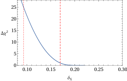
Figure 1: $\Delta\chi^{2}$ for varying degrees of allowed SU(3)_F breaking $\delta_{X}$. $\Delta\chi^{2}=1\,(25)$, i.e. $1\,(5)\sigma$, corresponds to $\delta_{X}=0.17(0.09)$, indicated by the dashed(dotted) line, and $\Delta\chi^{2}<1\times 10^{-3}$ is reached for $\delta_{X}>0.2$.

The current experimental status of the relevant branching ratio measurements is shown in Table 3. For $B_{s}$ decays, due to $\Delta\Gamma_{s}\neq 0$, we have to take into account a correction factor for the relation between the “theoretical” branching ratio at $t=0$ and the “experimental” time-integrated branching ratio De Bruyn et al. (2012). The implications of $\Delta\Gamma_{s}\neq 0$ for $B_{s}\rightarrow D_{s}^{\pm}K^{\mp}$ have been discussed in detail in Ref. Fleischer and Malami (2022) and we use the “theoretical” $\mathcal{B}(\overline{B}_{s}^{0}\rightarrow K^{-}D_{s}^{+})$ as extracted from the experimental data therein. This amounts to a correction of $\sim 14\%$ vs. the “experimental” value $\mathcal{B}(\overline{B}_{s}^{0}\rightarrow K^{\mp}D_{s}^{\pm})=(2.25\pm 0.12)\cdot 10^{-4}$ Workman et al. (2022), see Refs. Fleischer and Malami (2022); De Bruyn et al. (2013) for details.

The decay $\bar{B}_{s}^{0}\rightarrow\pi^{-}D_{s}^{+}$ is flavor-specific, see Ref. Gershon et al. (2022) for a detailed discussion. Therefore, in this case the correction factor accounting for the non-vanishing $B_{s}$ width difference $\Delta\Gamma_{s}$ reads $1-y_{s}^{2}$ De Bruyn et al. (2012), with Amhis et al. (2023b)

$$y_{s}=\Delta\Gamma_{s}/(2\Gamma_{s})=0.064\pm 0.0035\,,$$ (31)

and the average $B_{s}$ width $\Gamma_{s}$. As $y_{s}^{2}\sim 0.004$, and the relative uncertainty of $\bar{B}_{s}^{0}\rightarrow\pi^{-}D_{s}^{+}$ is an order of magnitude larger, we neglect the effect of the non-vanishing width difference for this decay.

The decay channel $\overline{B}_{s}^{0}\rightarrow K^{0}D^{0}$ interferes with $B_{s}^{0}\rightarrow\overline{K}^{0}D^{0}$ through $B_{s}$ and kaon mixing. However, the latter decay channel is relatively suppressed by $\mathcal{O}(\lambda^{2})$ Gronau et al. (1995). Therefore, compared to the current relative error of $\sim 20\%$ for $\mathcal{B}(\overline{B}_{s}^{0}\rightarrow K^{0}D^{0})$, we neglect the effect of $\Delta\Gamma_{s}\neq 0$ in this case, too.

For our global fit, we assume that

$$|T_{i}/T| \leq\delta_{X}\,,$$ (32)

$$|C_{i}/C| \leq\delta_{X}\,,$$ (33)

$$|E_{i}/E| \leq\delta_{X}\,,$$ (34)

where $\delta_{X}$ is a measure of the allowed SU(3)_F breaking which we set to

$$\delta_{X} =0.3\,.$$ (35)

We have altogether ten experimental data points (two branching ratios not yet being measured) and 17 real theory parameters, of which nine are magnitudes and eight are strong phases. However, we also have six constraints Eqs. (32)–(34) on these parameters and it is indeed non-trivial if the data is in agreement with these constraints.

At the global minimum, for our null hypothesis we find $\chi^{2}=0$, i.e. a perfect fit to the data, meaning that the data can be explained with SU(3)_F breaking of $\delta_{X}=30\%$, as we expect. In order to demonstrate the non-triviality of this result, we show in Fig. 1 the resulting $\Delta\chi^{2}$ profile as a function of $\delta_{X}$, compared to our null hypothesis.

Our fit results for $\delta_{X}=0.3$ are presented in Tables 4, 5, and 6. All errors are obtained by profiled-$\chi^{2}$ scans. Since the SU(3)_F system is under-constrained, with more parameters than observables, it has a high degree of degeneracy. The parameter scans show non-Gaussianity, and appear flat around the minimum while sharply increasing near parameter boundaries. For that reason we quote parameter ranges instead of a central point with errors.

For completeness, in Table 7 we also show updated fits of the $B\rightarrow D\pi$ and $B\rightarrow DK$ isospin systems, which are in agreement with and more precise than previous results in Refs. Neubert and Petrov (2001); Xing (2002); Cheng (2002); Chiang and Rosner (2003); Mantry et al. (2003) and Colangelo and Ferrandes (2005); Xing (2003); Mantry et al. (2003), respectively, thanks to the steady experimental progress Abe et al. (2001); Ahmed et al. (2002); Krokovny et al. (2003); Aubert et al. (2004, 2007, 2006a, 2006b); Horii et al. (2008); Lees et al. (2011); Aaij et al. (2013); Kato et al. (2018); Aaij et al. (2021b); Bloomfield et al. (2022); Waheed et al. (2022).

We make the following observations:

• The SU(3)_F limit is excluded at $>5\sigma$, mainly triggered by the need for SU(3)_F breaking in the tree diagrams, which is also $>5\sigma$. SU(3)_F breaking in the $C$ diagrams is needed at $2.4\sigma$, while we are not yet sensitive to SU(3)_F breaking in $E$ diagrams.

• Compared to Ref. Colangelo and Ferrandes (2005), where the topological amplitudes are extracted in the SU(3)_F limit, and to Ref. Chiang and Senaha (2007), where partial SU(3)_F breaking effects are taken into account, we find that the general features of the results for $|C/T|$ and $|E/T|$ obtained in Colangelo and Ferrandes (2005); Chiang and Senaha (2007) are confirmed when including the first order corrections in full generality, however, the additional parameters result in larger errors for $|C/T|$.

• The data can be described perfectly well with SU(3)_F breaking of $\sim 20\%$. This conclusion holds independently of employing parameter-dependent or parameter-independent measures of SU(3)_F breaking, see Fig. 1 and Table 6. Our observation agrees with the conclusions of studies of SU(3)_F breaking based on factorization Bordone et al. (2020); Fleischer et al. (2011), where the factorizable SU(3)_F breaking from the decay constants can be estimated as $f_{K}/f_{\pi}-1\sim 20\%$ Aoki et al. (2022), see also Ref. Jung and Mannel (2009).

• The SU(3)_F-breaking effects in $T$, $C$ and $E$ do not add up constructively in order to produce larger SU(3)_F-breaking effects. This can be seen from the SU(3)_F-breaking measure $\varepsilon_{4}$, which relates the $U$-spin pair $\overline{B}^{0}\to\pi^{-}D^{+}$ and $\overline{B_{s}}^{0}\to K^{-}D_{s}^{+}$, see Table 6.

• The $B\rightarrow D\pi$ isospin amplitude ratio is still in agreement with the heavy-quark limit estimate Neubert and Petrov (2001)

  $$|A_{1/2}/A_{3/2}| \overset{\text{HQ-limit}}{=}1+\mathcal{O}(\Lambda_{\mathrm{QCD}}/m_{c})\,.$$ (36)

• The data implies that the ratio $|E/T|$ is more strongly suppressed than $|C/T|$. However, $|C/T|$ is rather large compared to the expectation from $1/N_{c}$ counting Gronau et al. (1995). The obtained knowledge of $|E/T|$ is mainly driven by the constraint from

  $$\left|\frac{\mathcal{A}(\overline{B}^{0}\rightarrow K^{-}D_{s}^{+})}{\mathcal{A}(\overline{B}^{0}\rightarrow\pi^{-}D^{+})}\right|=\left|\frac{E+E_{2}}{T+E}\right|\,,$$ (37)

  together with $\left|E_{2}/E\right|<0.3$.

• The phases $\phi_{C}$ and $\phi_{E}$ are sizable, indicating large rescattering effects. The phases of the SU(3)_F-breaking topologies are not yet very well known.

• Due to lack of data we can not yet test the isospin relation $s_{1}=1$, see Eqs. (23, 29). From our fit we obtain the corresponding yet unmeasured branching ratios as

  $$\quad\mathcal{B}(\bar{B}_{s}^{0}(t=0)\rightarrow\pi^{-}D^{+})$$

  $$=2\mathcal{B}(\bar{B}_{s}^{0}(t=0)\rightarrow\pi^{0}D^{0})$$

  $$=[0.4,6.0]\cdot 10^{-6}\,.$$ (38)

  The interfering $B_{s}$ decays into the same final states are in this case of the same order in Wolfenstein-$\lambda$, like it is also the case for $\overline{B}_{s}^{0}\rightarrow K^{\mp}D_{s}^{\pm}$ decays, see above. Estimating the impact from $\Delta\Gamma_{s}\neq 0$ as $\sim 20\%$, as suggested by the size of the effect for $\mathcal{B}(\overline{B}_{s}^{0}\rightarrow K^{-}D_{s}^{+})$, we predict

  $$\mathcal{B}(\bar{B}_{s}^{0}\rightarrow\pi^{-}D^{+}) =2\mathcal{B}(\bar{B}_{s}^{0}\rightarrow\pi^{0}D^{0})$$

  $$=[0.3,7.2]\cdot 10^{-6}\,.$$ (39)

  Future measurements of $\mathcal{B}(\overline{B}^{0}_{s}\to\pi^{-}D^{+})$ and $\mathcal{B}(\overline{B}^{0}_{s}\to\pi^{0}D^{0})$ would allow to test their isospin symmetry relation and at the same time improve the bounds on $|E/T|$.

IV Conclusions

Motivated by recently found discrepancies between experimental data and QCD factorization, we study the anatomy of a plain SU(3)_F expansion in $B\rightarrow DP$ decays as extracted from the data, with no further theory assumptions. We find that, although the SU(3)_F limit is excluded by $>5\sigma$, the data can be explained with SU(3)_F breaking of $\sim 20\%$,  i.e., the SU(3)_F expansion works to the expected level.

As is well known, SU(3)_F is an approximate symmetry of QCD as the light ($u$, $d$, $s$) quark masses are not equal to each other though they (especially $u$ and $d$) are small compared to $\Lambda_{\mathrm{QCD}}$. So when predictions made by assuming SU(3)_F are not upheld experimentally, it often becomes important to estimate the size of SU(3)_F breaking before invoking new physics.

As one more piece in the puzzle, our results inform future theoretical and experimental work. By considering the complete system of decays related by the SU(3)_F symmetry, we show unambiguously that the underlying issue is not connected to SU(3)_F breaking, as suggested by the ratio in Eq. (1), which is in agreement with the data. In a scenario beyond the SM (BSM), any new physics model designed to explain the deviations has therefore to respect the SU(3)_F structure of the SM operators, implying bounds on the hierarchy between BSM couplings to the first and second generation of quarks.

It would be very interesting to complete the picture in the future by testing the isospin sum rule between $\mathcal{B}(\bar{B}_{s}^{0}\rightarrow\pi^{-}D^{+})$ and $\mathcal{B}(\bar{B}_{s}^{0}\rightarrow\pi^{0}D^{0})$, as well as the SU(3)_F sum rule between $\mathcal{B}(\bar{B}^{0}\rightarrow K^{-}D_{s}^{+})$ and $\mathcal{B}(\bar{B}_{s}^{0}\rightarrow\pi^{-}D^{+})$, see Eqs. (23, 24, 29). In order to achieve this, measurements of the suppressed decay modes $\bar{B}_{s}^{0}\rightarrow\pi^{-}D^{+}$ and $\bar{B}_{s}^{0}\rightarrow\pi^{0}D^{0}$ are necessary, whose branching ratios we predict in Eq. (39).

The LHCb Upgrade II experiment has strong prospects for these modes. Run 5 of the LHC, scheduled for 2035, will see LHCb operating at instantaneous luminosities an order of magnitude greater than previously and accumulating a data sample corresponding to a minimum of 300 fb^-1. This increase in luminosity will be accompanied by improvements to the electromagnetic calorimeter granularity and energy resolution greatly enhancing sensitivity to modes with neutral particles in the final state Aaij et al. (2018).

From our parameter extraction in Table 4 it is evident that many of the SU(3)_F breaking parameters are basically unconstrained. Future more precise branching ratio data would allow to test the pattern of the SU(3)_F anatomy with much more accuracy. Besides the unmeasured decay channels $\bar{B}_{s}^{0}\rightarrow\pi^{-}D^{+}$ and $\bar{B}_{s}^{0}\rightarrow\pi^{0}D^{0}$, there is a lot of room for improvement left in the channels $\bar{B}^{0}\rightarrow K^{-}D_{s}^{+}$, $\bar{B}_{s}^{0}\rightarrow K^{0}D^{0}$, $\bar{B}^{0}\rightarrow\bar{K}^{0}D^{0}$ and $\bar{B}_{s}^{0}\rightarrow K^{-}D_{s}^{+}$, all of which still have relative branching ratio uncertainties of $>10\%$. Being a general characteristic of symmetry-based methods, we need improvements in several decay channels in order to obtain a complete picture of the underlying dynamics of $B\rightarrow DP$ decays.