An Efficient Difference-of-Convex Solver for Privacy Funnel

Abstract

We propose an efficient solver for the privacy funnel (PF) method, leveraging its difference-of-convex (DC) structure. The proposed DC separation results in a closed-form update equation, which allows straightforward application to both known and unknown distribution settings. For known distribution case, we prove the convergence (local stationary points) of the proposed non-greedy solver, and empirically show that it outperforms the state-of-the-art approaches in characterizing the privacy-utility trade-off. The insights of our DC approach apply to unknown distribution settings where labeled empirical samples are available instead. Leveraging the insights, our alternating minimization solver satisfies the fundamental Markov relation of PF in contrast to previous variational inference-based solvers. Empirically, we evaluate the proposed solver with MNIST and Fashion-MNIST datasets. Our results show that under a comparable reconstruction quality, an adversary suffers from higher prediction error from clustering our compressed codes than that with the compared methods. Most importantly, our solver is independent to private information in inference phase contrary to the baselines.

I Introduction

The privacy funnel (PF) method attracts increasing attention recently, driven by the need for enhanced data security as modern machine learning advances. However, due to the non-convexity of the involved optimization problem, the strict Markov constraint, and the requirement of full knowledge of a probability density, the PF problem is well-known to be difficult to solve. In the PF method, the goal is to solve the following optimization problem [1]:

$$\underset{P(Z|X)\in\Omega_{Z|X}}{\min}\, I(Z;Y),$$

subject to $$I(Z;X)\geq\eta_{X},$$ (1)

where $\eta_{X}$ denotes a control threshold. In the above problem, the joint distribution $P(X,Y)$ is assumed to be known and the random variables satisfy the Markov chain $Y\rightarrow X\rightarrow Z$. Here, $Y$ is the private information; $X$ the public information and $Z$ is the released (compressed) codes; $I(Z;X)$ denotes the mutual information between two random variables $Z$ and $X$. In (1), the variables to optimize with are the stochastic mappings $P(Z|X)$ with $\Omega_{Z|X}$ denotes the associated feasible solution set. The aim of the problem is to characterize the fundamental trade-off between the privacy leakage and the utility of the released information. One of the challenges in solving (1) is the non-convexity of the problem. It is well-known that the mutual information $I(Z;X)$ with known marginal $P(X)$ is a convex function with respect to $P(Z|X)$ [2]; Additionally, due to the Markov relation, $I(Z;Y)$ is a convex function of $P(Z|X)$ as well. Together, (1) minimizes a convex objective under a non-convex set. Previous solvers for PF address the non-convexity by restricting the feasible solution set further for efficient computation. Both [1] and [3] consider discrete settings and focus on deterministic $P(z|x)$, i.e., a realization of $x\in\mathcal{Z}$ belongs to a single cluster $z\in\mathcal{Z}$ only. They propose greedy algorithms to solve the reduced problem and differ in choosing the subset of $\mathcal{Z}$ to combine with. However, the imposed restriction limits the characterization of the privacy-utility trade-off. In our earlier work [4], we propose a non-convex alternating direction methods of multipliers (ADMM) solver for PF which is non-greedy, but it suffers from slow convergence [5].

Another challenge of PF is knowing the joint distribution $P(X,Y)$. Overcoming this is important for practical application of the method as $P(X,Y)$ is prohibitively difficult to obtain in general. Nonetheless, it is relatively easy to obtain samples of the joint distribution, which become a training dataset as an indirect access to $P(X,Y)$. Recently, inspired by the empirical success of information theoretic-based machine learning, several works have attempted to extend the PF method through the theory of variational inference [6]. In [7], the conditional mutual information form of PF due to $I(Y;Z)=I(X;Z)-I(X;Z|Y)$ is adopted, whose variational surrogate bound is estimated with empirical samples. In [8] a similar formulation is adopted, but they restrict the parameter space and implement a generative deep architecture for interchangeable use of the empirical and the generated $Y$ samples for estimation instead. However, owing to the dependency of the private information $Y$ in estimating $I(X;Z|Y)$, these previous solvers violate the fundamental Markov relation in PF method. Consequently, samples of $X,Y$ are required for their solvers which means supervision is required in both model training and inference phases.

Different from the previous works, we focus on the computation efficiency of PF in both known and unknown (empirical samples available) joint distribution settings based on the difference-of-convex (DC) structure of (1). In known joint distribution settings, inspired by the difference-of-convex algorithm (DCA), we propose a novel efficient PF solver with closed-form update equation. In our evaluation, the proposed solver not only covers solutions obtained from the state-of-the-art solvers but also attains non-trivial solutions that the compared greedy solvers are infeasible to reach. In unknown $P(X,Y)$ settings, our DC method complies with the fundamental Markov relation, therefore requires public information $X$ only in inference phase in contrast to previous approaches. We implement our solver with deep neural networks and evaluate the model on MNIST and Fashion-MNIST datasets. In all evaluated datasets, our approach outperforms the state-of-the-art. Specifically, under a comparable reconstruction quality of the public information $X$, an adversary’s clustering accuracy (leakage of the private information $Y$) with the released codes $Z$ of ours is significantly lower than the compared approaches.

Notations

Upper-case letters denote random variables (RVs) and lower-case letters are their realizations. The calligraphic letter denotes the sample space, e.g., $x\in\mathcal{X}$ with cardinality $|\mathcal{X}|$. The vectors and matrices are denoted in bold-face symbols, i.e., $\boldsymbol{x},\boldsymbol{X}$ respectively. We denote the conditional probability mass function as a long vector:

$$\boldsymbol{p}_{z|x}:=\begin{bmatrix}P(x_{1}|z_{1})&P(x_{1}|z_{2})&\cdots&P(x_{|\mathcal{X}|}|z_{|\mathcal{Z}|})\end{bmatrix}^{T}.$$ (2)

The Kullback-Leibler divergence of two measurable proper densities $\mu,\nu$ is denoted as $D_{KL}[\mu\parallel\nu]$ [2].

II A Difference-of-Convex Algorithm for Privacy Funnel

For simplicity, we focus on discrete random variables settings in this section. We start with a summary of DC programming and refer to the excellent review [9] for the development and recent advances of the DC method. For a DC program, the canonical form is given by:

$$w^{*}=\underset{w\in\mathcal{W}}{\arg\min}\,f(w)-g(w),$$ (3)

where $f,g$ are functions of $w$, and $\mathcal{W}$ denotes the feasible solution set of $w$. (3) relates to the PF method because (1) can be re-written into an unconstrained PF Lagrangian:

$$\mathcal{L}_{PF}:=I(Z;Y)-\beta I(Z;X),$$ (4)

where $\beta>0$ is a multiplier. When $P(X,Y)$ is known, the above reveals a DC structure. This is because $I(Z;X)$ is convex w.r.t. $P(Z|X)$ for known $P(X)$, and $-H(Z|Y)$ is convex w.r.t. $P(Z|X)$ as the Markov relation $P(Z|Y)=\sum_{x\in\mathcal{X}}P(Z|x)P(x|Y)$ along with known $P(Y)$ implies convexity [2]. The DC structure of (4) can be leveraged for efficient optimization. The idea is to use the first order approximation of the concave part of the objective function, resulting in a convex sub-objective. Then we iteratively minimize the convex surrogate sub-objective until the loss saturates. The monotonically decreasing loss values is assured due to the convexity of the sub-objective functions but the optimality of the converged solution is lost due to the non-convexity of the overall objective. There are well-developed efficient solvers for DC problems in literature, known as the Difference-of-Convex Algorithm (DCA). However, one of the key challenges in solving DC problems with DCA is that there exist infinitely many combinations of DC pairs [9]. Furthermore, a poorly chosen pair may result in slow convergence and numerical instability. We address it by proposing the following DC separation:

$$f(\boldsymbol{p}_{z|x}): = -H(Z|Y),$$ (5a)

$$g(\boldsymbol{p}_{z|x}): = -H(Z)+\beta I(Z|X),$$ (6a)

Then we apply (5a) to DCA:

$$\boldsymbol{p}^{k+1}_{z|x}:=\underset{\boldsymbol{p}_{z|x}\in\Omega_{z|x}}{\arg\min}\,f(\boldsymbol{p}_{z|x})-\langle\nabla g(\boldsymbol{p}^{k}_{z|x}),\boldsymbol{p}_{z|x}-\boldsymbol{p}^{k}_{z|x}\rangle,$$ (7)

where the superscript $k$ denotes the iteration counter. For known $P(X,Y)$ in discrete settings, (7) can be expressed as a linear equation (see Appendix A):

$$\boldsymbol{B}_{y|x}\log{\boldsymbol{p}_{z|y}}=\log{\boldsymbol{p}^{k}_{z}}+\beta\log{\frac{\boldsymbol{p}^{k}_{z|x}}{\boldsymbol{p}^{k}_{z}}},$$ (8)

where $\boldsymbol{B}_{y|x}$ denotes the matrix-form of $P(Y|X)$ with the $(i,j)$-entry represents $P(y_{i}|x_{j})$. We follow the common assumption in private source coding literature and assume that $\boldsymbol{B}_{y|x}$ is full-row rank [10, 11, 12, 13, 14]. Under this assumption, the pseudo-inverse of $\boldsymbol{B}_{y|x}$ exists, and we denote its Moore-Penrose pseudo inverse as $\boldsymbol{B}^{\dagger}_{y|x}:=(\boldsymbol{B}_{y|x}^{T}\boldsymbol{B}_{y|x})^{-1}\boldsymbol{B}_{y|x}^{T}$. Then (8) reduces to:

$$\tilde{\boldsymbol{p}}_{z|y}\propto\exp\{\boldsymbol{B}^{\dagger}_{y|x}\boldsymbol{c}^{k}_{z|x}\},$$ (9)

where $\boldsymbol{c}^{k}_{z|x}:=\log{\boldsymbol{p}^{k}_{z}}+\beta\log{\frac{\boldsymbol{p}^{k}_{z|x}}{\boldsymbol{p}^{k}_{z}}}$, $\tilde{\boldsymbol{p}}_{z|y}$ denotes the un-normalized probability vector and $\propto$ represents proportional to. After normalization, followed by the Markov relation, we have $\boldsymbol{A}_{x|y}\boldsymbol{p}_{z|x}=\boldsymbol{p}_{z|y}$ with $\boldsymbol{A}_{x|y}$ denotes the matrix-form of $P(X|Y)$. Therefore, the insight from applying DCA to PF gives an update equation:

$$\boldsymbol{A}_{x|y}\boldsymbol{p}_{z|x}=\boldsymbol{\phi}(\boldsymbol{B}_{y|x}^{\dagger}\boldsymbol{c}^{k}_{z|x}):=\boldsymbol{q}^{k}_{z|y},$$ (10)

where the $z\in\mathcal{Z}$ element is given by $\phi_{z}=e^{z}/\sum_{z^{\prime}\in\mathcal{Z}}e^{z^{\prime}}$. In practice, $\boldsymbol{\phi}$ is implemented as a softmax function. The above implies that the update of $\boldsymbol{p}_{z|x}$ from step $k$ to step $k+1$ requires solving the linear equation (10). However, since $\boldsymbol{B}_{y|x}$ is only full-row rank, (10) is an under-determined linear program over non-negative simplice (convex set). Heuristically, one would prefer a solution with the lowest complexity, which is often achieved by imposing $q$-norm (e.g., $q\in\{0,1,2\}$) constraints as regularization [15]. Based on this intuition, we therefore state the iterative update equation as the following optimization problem:

$$\underset{\boldsymbol{p}_{z|x}\in\Omega_{z|x}}{\min}\, \lVert\boldsymbol{p}_{z|x}\rVert_{q},$$

subject to $$\boldsymbol{A}_{x|y}\boldsymbol{p}_{z|x}=\boldsymbol{q}^{k}_{z|y},$$ (11)

where $\lVert\boldsymbol{v}\rVert_{q}:=(\sum_{v\in\mathcal{V}}|v|^{q})^{1/q}$. Similar to relaxing the “hard” constraints in classical regression problems, which allows for the application of significantly more efficient algorithms, we solve the following relaxed problem of (11) where a soft constraint is considered instead:

$$\boldsymbol{p}^{k+1}_{z|x}:=\underset{\boldsymbol{p}_{z|x}\in\Omega_{z|x}}{\arg\min}\, \frac{1}{2}\lVert\boldsymbol{A}_{x|y}\boldsymbol{p}_{z|x}-\boldsymbol{q}_{z|y}^{k}\rVert^{2}_{2}+\alpha\lVert\boldsymbol{p}_{z|x}\rVert_{q},$$ (12)

where $\alpha>0$ is a relaxation coefficient. It is straightforward to see that the optimization problem is relaxed because of the tolerance of an approximation error of the linear equation. Remarkably, (11) is closely related to classical regression problems such as Ridge regression [16], LASSO [17], and sparse recovery [18]. But the key difference is that in (11) and (12), the feasible solution set $\Omega_{z|x}$ is the probability simplice. For $q=2$, since here (12) corresponds to a convex optimization problem, each step can be solved efficiently with off-the-shelf ridge regression solvers [19]. As for $q=1$ (convex surrogate for $q=0$), however, the LASSO solver [17] does not work well. This is because $\lVert\boldsymbol{p}_{z|x}\rVert_{1}=\sum_{x\in\mathcal{X}}|\boldsymbol{p}_{Z|x}|=|\mathcal{X}|$, since $\sum_{z\in\mathcal{Z}}P(z|x)=1,\forall x\in\mathcal{X}$ always. To address this, we provide an alternative approach for sparse recovery ($q=0$) with details referred to Appendix B:

$$l^{k+1}_{z|x}:=\underset{l_{z|x}\in\mathcal{H}_{z|x}}{\arg\min}\,\frac{1}{2}\lVert{lse}_{x}(l_{x|y}+l_{z|x})-l^{k}_{\phi}\rVert^{2}+\alpha\lVert l_{z|x}\rVert_{1},$$ (13)

where $l_{x|y}:=\log{\boldsymbol{p}_{x|y}}$, $lse(x):=\log\sum_{x\in\mathcal{X}}\exp\{x\}$ is the log-sum-exponential function; $\mathcal{H}_{z|x}$ is the feasible set for $l_{z|x}\in[-M,-m]$ for some $M>m>0$ such that $\sum_{z\in\mathcal{Z}}\exp\{l_{z|x}\}=1,\forall x\in\mathcal{X}$; the subscript denotes the variable for summation, and $l_{\phi}^{k}:=\log{\boldsymbol{\phi}(\boldsymbol{B}_{y|x}^{\dagger}\boldsymbol{c}^{k}_{z|x})}$. Then after solving (13), we can project the obtained $l_{z|x}$ to a feasible solution $\boldsymbol{p}_{z|x}$ through a softmax function: $\boldsymbol{p}_{z|x}=\text{Softmax}(l_{z|x})$.

For both implementations, the proposed solver guarantees convergence to a local stationary point.

Theorem 1

For both implementations (12) ($q=2$) and (13), the sequence $\{\boldsymbol{p}_{z|x}^{k}\}_{k\in\mathbb{N}}$, obtained from (7), converges to a stationary point $\boldsymbol{p}_{z|x}^{*}$ such that $\nabla f(\boldsymbol{p}^{*}_{z|x})=\nabla g(\boldsymbol{p}^{*}_{z|x})$ with $f,g$ defined in (5a).

Proof:

See Appendix D. ∎

III Extension to Unknown Distributions

The main difficulty in applying PF is the full knowledge of the joint distribution $P(X,Y)$ [1]. In (12), this corresponds to defining the operators $\boldsymbol{A}_{x|y}$ and $\boldsymbol{B}_{y|x}^{\dagger}$. Without knowing $P(X,Y)$, these operators are intractible. To address this, we leverage the DC structure of the PF problem again, but now take expectation with respect to $P(Z,X)=P(Z|X)P(X)$ on the update equation which reveals that (see Appendix C):

$$I(Z;Y)+D_{KL}[P_{z}\parallel P_{z}^{k}]-\beta\mathbb{E}_{z,x}\left[\log{P^{k}(X|Z)}\right]=0,$$ (14)

where the superscript $k$ denotes the iteration counter. The above update equation implies that the step $k+1$ solution $P^{k+1}(Z|X)$ is obtained from solving (14), given the previous step $k$ solution $P^{k}(Z|X)$.

The expectation form (14) is useful because the computationally prohibitive knowledge of $P(X,Y)$ can be approximated efficiently through the theory of the variational inference, followed by Monte-Carlo sampling [20, 6]. The derived surrogate bound involves an auxiliary variable, which corresponds to the released information $Z$, and is associated with a variational distribution to be designed. For the mutual information $I(Z;Y)=H(Y)-H(Y|Z)$:

$$H(Y|Z)\leq\mathbb{E}_{y,z;\phi}\left[\log{\frac{1}{Q_{\phi}(Y|Z)}}\right],$$ (15)

where the above surrogate bound is tight when $Q_{\phi}(Y|Z)=P(Y|Z)$. As for the other terms of (14), we parameterize $P_{\theta}(Z)=\mathcal{N}(\boldsymbol{0},\text{diag}(\boldsymbol{\sigma}_{\theta}^{2}))$ as standard Gaussian and $P_{\phi}(X|Z)=\mathcal{N}(\boldsymbol{\mu}_{\phi}(\boldsymbol{z}),\boldsymbol{I})$ as conditional Gaussian distributions. This transforms the intractible problem into a standard parameter estimation. Also, we parameterize the encoder $P_{\theta}(Z|X)$, corresponding to the expectation operator in (14), through the evident lower bound technique as adopted in the variational autoencoders (VAE) [20]. Here, we have $P_{\theta}(Z|X)\sim\mathcal{N}(\boldsymbol{\mu}_{\theta}(\boldsymbol{x}),\boldsymbol{\Sigma}_{\theta}(\boldsymbol{x}))$. Combining the above, we propose the following alternating solver:

$$\phi^{*}:=\underset{\phi\in\Phi}{\arg\min}\, -\beta\mathbb{E}_{x,z;\theta^{k}}\left[\log{P_{\phi}(X|Z)}\right]$$ (16a)

$$-\mathbb{E}_{y,z;\theta^{k}}\left[\log{Q_{\phi}(Y|Z)}\right],$$

$$\theta^{k+1}:=\underset{\theta\in\Theta}{\arg\min}\, \frac{1}{2}\lVert I_{\phi^{*};\theta}(Z;Y)+D_{KL}[P_{z;\theta}\parallel P_{z;\theta^{k}}]$$ (17a)

$$-\beta\mathbb{E}_{z,x;\theta}\left[\log{P_{\phi^{*}}}(X|Z)\right]\rVert_{2}^{2}$$

$$+\alpha\mathbb{E}_{x}\left[D_{KL}[P_{z|x;\theta}\parallel r_{Z}]\right],$$

where $r_{Z}=\mathcal{N}(\boldsymbol{0},\boldsymbol{I})$ is a reference probability density function, regularizing the encoder; and $\alpha>0$ is a control threshold. Essentially, we alternate between fitting the empirical samples of $X,Y$ (16a) and solve the DCA update sub-problem with an extra regularization term (17a). The two steps are repeated until a pre-determined number of iterations is reached.

The optimization of (16a) is efficient. Each of the two KL divergence terms are computed between two Gaussian densities which has closed-form expression [21]; the parameterized $P_{\phi}(X|Z)$ and $Q_{\phi}(Y|Z)$ (hence $I(Z;Y)\approx H(Y)-H_{\phi}(Y|Z)$) can be estimated with mean-squared error (MSE) and a categorical cross entropy loss respectively. Finally, two remarks are in order:

• While we adopt the variational inference similar to the previous works [7, 8]. We apply it on the expectation form of the proposed DC update equation (14), not on the PF Lagrangian nor on $I(X;Z|Y)$.

• The parameterization of (16a) can be extended to other density functions such as Laplace, Bernoulli and exponential distributions [22, 23].

IV Evaluation

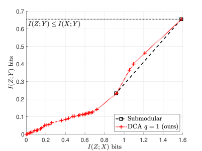
(a) DCA (13) with $q=1$ versus Submodular [3]

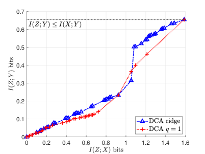
(b) DCA (13) with $q=1$ versus (12) with $q=2$ (ridge)

Figure 1: Comparing the characterization of the privacy-utility trade-off between the proposed DCA solvers and the state-of-the-art method [3]. Under known joint distribution of $P(X,Y)$ settings, given by (18).

IV-A Known Distribution

The joint distribution we consider in this part is given by:

$$\boldsymbol{P}_{Y|X}=\begin{bmatrix}0.90&0.08&0.40\\ 0.025&0.82&0.05\\ 0.075&0.10&0.55\end{bmatrix},\quad\boldsymbol{p}_{X}=\begin{bmatrix}\frac{1}{3}\\ \frac{1}{3}\\ \frac{1}{3}\end{bmatrix}.$$ (18)

Observe that the $y_{0},y_{1}$ of this distribution are easy to infer if observing $x_{0},x_{1}$ whereas there is ambiguity in inferring $y_{0},y_{2}$ if $x_{2}$ is observed instead.

The goal of our evaluation is to characterize the privacy-utility trade-off by plotting the lowest achieved $I(Z;Y)$ for an obtained $I(Z;X)$. The characterized trade-off is displayed as the information plane [1, 4], which depends on both $P(X,Y)$ and the algorithm used. We evaluate our DCA solver (5a) and compare it to the state-of-the-art [1, 3] when $P(X,Y)$ is known. These baselines only consider deterministic $P(z|x)=\boldsymbol{1}\{x\in z\}$, that is, $z$ categorizes $X$. Also, they are greedy algorithms that merge two or more $z\in\mathcal{Z}$ each step for a lower PF Lagrangian. Contrary to them, our solver is non-greedy with feasible solutions covers the (smoothed) probability simplice. For these baselines, it suffices to compare to the solver in [3] since the solver in [1] is a special case of it.

In the proposed solver (5a), the range of cardinality $|\mathcal{Z}|$ follows the Carathéodory Theorem, which is should satisfy $|\mathcal{Z}|\leq\max\{|\mathcal{X}|,|\mathcal{Y}|\}+1$ [24]. For each cardinality, we initialize $P(Z|X)$ by randomly sample a uniformly distributed source, followed by normalization to obtain a starting point. Then, we fix a trade-off parameter $\beta\in[0.1,10.0]$ and a regularization coefficient $\alpha\in[0.1,10.0]$, where each set consists of $16$ geometrically spaced points. For each set of hyperparameters, we run our solver until either the consecutive loss values satisfy $|\mathcal{L}^{k}-\mathcal{L}^{k+1}|\leq 10^{-6}$ or a maximum number of iterations $M=10^{4}$ is reached. This procedure is repeated for $10$ times. We compute the obtained metrics $I(Z;X),I(Z;Y)$ offline.

In Fig. 1a, our solver (5a) characterizes the trade-off better than the baseline solvers since we not only cover their solutions but achieve more non-trivial points that are infeasible to them. In Fig. 1b we compare the two proposed DCA solvers with different implementation of the inner problem, i.e., (12) with $q=2$ (ridge) versus (13) with $q=1$. While the ridge approach performs worse than the other solver in the characterization of the trade-off, it obtains a better trade-off point $I(Z;X)\approx 1$ bit and $I(Z;Y)\approx 0.3$ bits. Moreover, the ridge solver benefits from the optimized off-the-shelf solver [19], hence converges faster in our empirical evaluation. It is worth noting that both approaches outperform [3] in characterizing the trade-off under different regularization criterion, which is the strength of our DCA approach.

IV-B Unknown Distribution

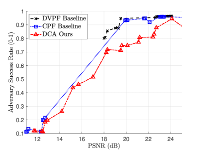
(a) MNIST

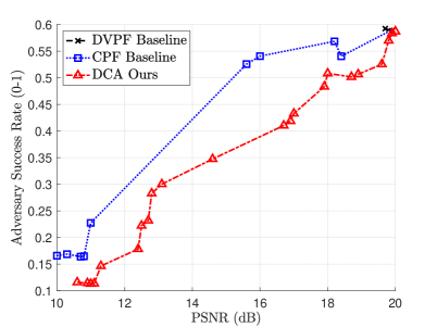
(b) Fashion-MNIST

Figure 2: Privacy-utility trade-off in unknown joint distribution settings. The proposed DCA solver is compared to the CPF [7] and DVPF [8] baselines.

For unknown $P(X,Y)$, we consider cases where empirical samples of the joint distribution are available (datasets) $\mathcal{D}_{N}:=\{(x^{(n)},y^{(n)})|(x^{(n)},y^{(n)})\sim P(X,Y)\}_{n=1}^{N}$. Our DCA solver is compared to the state-of-the-art Conditional Privacy Funnel (CPF) [7] and Deep Variational Privacy Funnel (DVPF) [8] baselines.

Datasets

we evaluate (17a) on two datasets: MNIST [25] and Fashion MNIST [26]. Both datasets consist of gray-scale images of $28\times 28$ pixels. Each pixel is normalized to the range $[0,1]$. Also, both datasets have labeled $60000$ training and $10000$ testing samples uniformly distributed between $10$ classes respectively. The data format of MNIST is images hand-written digits. Here, we let the digits $Y$ be the private information and the images are treated as the public information $X$. As for Fashion MNIST, it has $10$ categories of clothing. We refer to [26] for details. We set the categories as $Y$ and the gray-scale images as $X$.

The two datasets are applied to the scenario: a sender learns (supervised) an encoder-decoder pair with training dataset based on the PF objective. Then the sender encodes the $X$ of the testing set and the released compressed codes $Z$. A receiver observes the coded $Z$ and reconstruct $\hat{X}$ with $P_{\phi}(X|Z)$, obtained from a secure channel before the inference phase. Meanwhile, an adversary also observes the codes but does not know $P_{\phi}(X|Z)$. The adversary therefore learns $\hat{Y}$ from clustering $Z$. Here, we assume the cardinality of $|Y|$ is known for simplicity. In short, the legitimate users’ goal is to reconstruct $\hat{X}$ from $Z$ whereas the adversary clusters $Z$ and obtains $\hat{Y}$ that should reveal $Y$.

In our evaluation, we measure the reconstruction quality (utility) by the Peak Signal-to-Noise power Ratio (PSNR), defined as:$PSNR:=10\log{X_{\max}/MSE}$, where $X_{\max}$ is the maximum possible pixel value ($1$ in our case) and $MSE:=\frac{1}{N}\sum_{i=1}^{N}\lVert\boldsymbol{x}_{i}-\hat{\boldsymbol{x}}\rVert_{2}^{2}$. As for the privacy leakage, the adversary uses UMAP [27] to project $Z$ to a $\mathbb{R}^{2}$ space, followed by a KMeans clustering [19]. Note that this two-step approach achieves the state-of-the-art clustering performance for both MNIST and Fashion-MNIST datasets [27]. Then we compute the adversary’s success rate by an offline label matching.

Network Architecture

The proposed and compared methods are implemented as deep neural networks. Since our focus is on comparing the claimed PF objective, the encoders and decoders are almost aligned for all compared methods. For both methods, we implement the encoder as a neural network with fully connected (FC) layers whose outputs correspond to that of the standard VAE [20] encoder. We have a separate set of parameters for learning a prior $P_{\theta}(Z)=\mathcal{N}(\boldsymbol{0},\boldsymbol{\nu}_{\theta})$. As for the decoder, another neural network with FC layers is the common reconstruction module for both approaches. For the differences, our method has a separate linear classifier whereas the CPF baseline expand the decoder’s input by concatenating code samples $\boldsymbol{z}$ with the one-hot representation of $\boldsymbol{e}_{y}$ ($\boldsymbol{e}_{i}$ is the $i^{th}$ elementary vector).

We train a model for $100$ epochs with a learning rate at $3\times 10^{-4}$ using a standard ADAM optimizer [28]. The mini-batch size is $256$. For the dimension of $Z$, we vary $d_{z}\in\{32,64,128,256\}$ for both methods. The hyperparameter range for our method is set to $[5\times 10^{-4},5\times 10^{-2}]$ for both $\alpha$ and $\beta$ in (16a), whereas it is $[10^{-3},10]$ for the CPF baseline. Each hyperparameter pair is trained for $3$ time with a different random seed. Then we report the average in the results. The experiment details are included in Appendix E. For reproduction, our source codes in available online.

Results

The results are shown in Fig. 2, where the highest adversary success rate of an achieved PSNR for each method is reported. Note that the results include all combinations of the hyperparameters and the set of $d_{z}$. Fig. 2a corresponds to the MNIST dataset whereas the results for Fashion-MNIST dataset is shown in Fig. 2b. Clearly, in both figures, our method outperforms the CPF and DVPF baselines since the adversary has higher error rate in clustering $Z$ from our approach at a comparable reconstruction quality of $X$. Moreover, our approach better characterizes the privacy-utility trade-off better than both baselines. In addition to better robustness, in training phase, our approach is more efficient than the DVPF baseline since we require no parameters for generative and discriminative modules whose optimization follows by a complex six-step algorithm. As for in inference phase, our approach is completely independent to the private information, in sharp contrast to the CPF baseline. These demonstrate the strength of the proposed DCA method over the state-of-the-art baselines. Finally, for extended evaluation and visualization of the compressed features, we refer to Appendix F and Appendix G for details.

V Conclusions

We leverage the DC structure of the PF method and develop efficient solvers based on DCA. In known distribution settings, our solver resembles both ridge regression and sparse recovery. Empirically, our solver outperforms the state-of-the-art greedy solvers in characterizing the privacy-utility trade-off. As for the unknown distribution settings, the insights from the proposed DC approach allows compliance to the fundamental Markov relation, so that our approach applies to scenarios without labeled private information after training. The evaluation of the proposed solver of the MNIST and the Fashion-MNIST datasets demonstrates significantly improved privacy-utility trade-off than the compared methods. For future work, we empirically find that the compression ratio, defined as the ratio of the dimensionality of the release information to the public information, significantly affects the privacy-utility trade-off. A fundamental characterization in this direction will be the focus of a follow-up work.

Appendix A Derivation for a known joint distribution

Starting from (5a):

$$f(\boldsymbol{p}_{z|x}): = -H(Z|Y),$$

$$g(\boldsymbol{p}_{z|x}): = -H(Z)+\beta I(Z|X),$$

we note that the “linearized” part has the following closed-form expression from elementary functional derivative:

$$\frac{\partial g(\boldsymbol{p}_{z|x})}{\partial\boldsymbol{p}(z|x)}:=P(x)\left\{\log{P(z)}+1+\beta\log{\frac{P(z|x)}{P(z)}}\right\}.$$

Furthermore, when analyzing the first-order necessary condition of the right-hand-side of (7), we have:

$$\sum_{y\in\mathcal{Y}}P(y|x)\log{P(z|y)}=\left[\log{P^{k}(z)}+\beta\log{\frac{P^{k}(z|x)}{P^{k}(z)}}\right],$$

By definition, $\boldsymbol{B}_{y|x}$ is the matrix form of $P(Y|X)$ with $(i,j)$-entry $P(y_{i}|x_{j})$, so the above is equivalent to:

$$\boldsymbol{B}_{y|x}\log{\boldsymbol{p}_{z|y}}=\log{\boldsymbol{p}^{k}_{z}}+\beta\log{\frac{\boldsymbol{p}^{k}_{z|x}}{\boldsymbol{p}^{k}_{z}}}.$$

Appendix B Alternative Approach for Sparse Recovery

The transformation of the optimization problem (11) for the case $q=1$ to (13) is achieved through the following steps:

First, we change the variables from the conditional probabilities $\boldsymbol{p}_{z|x}$ to the log-likelihoods $l_{z|x}:=\log{\boldsymbol{p}_{z|x}}$. The benefit of this is that the domain becomes a half-space $l_{z|x}\in(-\infty,0]$, which is more straightforward for projection than the probability simplice for $\boldsymbol{p}_{z|x}$ as identified in [29]. Second, instead of finding the exact deterministic assignment, i.e., $P(z|x)=\boldsymbol{1}\{x\in\mathcal{Z}\}$, we impose smoothness conditions on the log-likelihoods, $-M\leq l_{z|x}\leq-m$ for some $M,m>0$. Lastly, we compute the Markov relation for $l_{z|x}$ as:

$$\log{\boldsymbol{p}_{z|y}}=\log\sum_{x\in\mathcal{X}}\exp\{l_{x|y}+l_{z|x}\},$$

where $l_{x|y}:=\log{\boldsymbol{p}_{x|y}}$. The above is implemented with a log-sum-exponential function $lse(x):=\log\sum_{x\in\mathcal{X}}\exp\{x\}$. Combining the above, we rewrite (12) ($q=1$) as:

$$l^{k+1}_{z|x}:=\underset{l_{z|x}\in\mathcal{H}_{z|x}}{\arg\min}\,\frac{1}{2}\lVert{lse}_{x}(l_{x|y}+l_{z|x})-l^{k}_{\phi}\rVert^{2}+\alpha\lVert l_{z|x}\rVert_{1}.$$

We therefore complete the transformation.

Appendix C Derivation for unknown joint distribution

Again, we start with the update equation:

$$\sum_{y\in\mathcal{Y}}P(y|x)\log{P(z|y)}=\left[\log{P^{k}(z)}+\beta\log{\frac{P^{k}(z|x)}{P^{k}(z)}}\right],$$

but now we take expectation with respect to $P(Z,X)=P(X)P(Z|X)$. The left-hand side is:

$$\mathbb{E}_{z,x}\left[\sum_{y\in\mathcal{Y}}P(y|X)\log{P(Z|y)}\right]$$

$$= \mathbb{E}_{y}\left[\sum_{z\in\mathcal{Z}}\sum_{x\in\mathcal{X}}P(z,x)P(x|Y)\log{P(z|Y)}\right]$$

$$= -H(Z|Y),$$

where the second equality is due to the Markov relation $Y\rightarrow X\rightarrow Z$. For the second term of (14), we have:

$$\mathbb{E}_{z}\left[\log{P^{k}(Z)}\right]=-H(Z)-D_{KL}\left[P_{z}\parallel P^{k}_{z}\right].$$ (19)

Combining the above with some re-arrangement, we have:

$$I(Z;Y)+D_{KL}[P_{z}\parallel P_{z}^{k}]-\beta\mathbb{E}_{z,x}\left[\log{P^{k}(X|Z)}\right]=0.$$

This completes the proof.

Appendix D Proof of Theorem 1

The proof follows that in [30, Theorem 1]. Which is included here for completeness.

By the first order necessary condition of the proposed DCA solver (7), we have:

$$\nabla f(p^{k+1})-\nabla g(p^{k})=0.$$ (20)

Denote the objective function as $\mathcal{L}(p)=f(p)-g(p)$ where $f,g$ are convex functions of $p$. We consider the following:

$$\mathcal{L}(p^{k})-\mathcal{L}(p^{k+1})$$

$$= f(p^{k})-g(p^{k})-f(p^{k+1})+g(p^{k+1})$$

$$\geq \langle\nabla f(p^{k+1})-\nabla g(p^{k}),p^{k}-p^{k+1}\rangle,$$

where the first inequality follows from the convexity of $f$ and $g$. Then by applying (20), we show that:

$$\mathcal{L}(p^{k})-\mathcal{L}(p^{k+1})\geq 0.$$ (21)

The above implies that the consecutive updates from (7) results in a non-increasing sequence of the objective values. For $k\geq K_{0}\in\mathbb{N}$ sufficiently large, we have a sequence of $\{p^{k}\}_{k\geq K_{0}}$ such that $\{\mathcal{L}(p^{k})\}_{k\geq K_{0}}$ converges to a $\mathcal{L}^{*}$ as $k\rightarrow\infty$. Denote the converged solutions $p^{*}\in\Omega^{*}$ where $\Omega^{*}:=\{p|\mathcal{L}(p)=\mathcal{L}^{*}\}$, then $\Omega^{*}$ is a set of stationary points whose objective value is $\mathcal{L}^{*}$. Now, because $\mathcal{L}$ is non-convex, $\Omega^{*}$ could include both local and global stationary points.

The above results do not directly apply to the proposed DCA solver because here we have two intermediate optimization problems (12) with $q=2$ and (13). Interestingly, both (12) and (13) are convex optimization problems, since the log-sum-exponential function and the $q$-norms for $q\in\{1,2\}$ are all convex functions. Therefore, the convexity assures convergence to the global optimum for the intermediate problems. Combining the above, the proof is complete.

Appendix E Experiment Details

We implement all compared solvers in Section IV-B as follows. For the hardware, we run our prototype on a commercial computer with an Intel i5-9400 CPU and one Nvidia GeForce GTX 1650 Super GPU with 16GB memory. As for the software, we implement all solvers with PyTorch. All methods are optimized with a standard ADAM optimizer [28] with a fixed learning rate of $3\times 10^{-4}$ for $100$ epochs, and we configure the mini-batch size to $256$. In Table I we list the number of parameters of the proposed solver with different dimensionality of $Z$.

TABLE I: Number of Trainable Parameters versus the code length.

$d_{z}$	Number of Parameters
$32$	$1084742$
$64$	$1133190$
$128$	$1230086$
$256$	$1423878$

As for the off-the-shelf software: UMAP and KMeans, the default configuration is adopted. We refer to the references for details [27, 19].

For both the proposed and compared methods, the deep neural network architectures are described as follows: the encoder is implemented as a multi-layer perceptron (MLP) with $784\rightarrow 500\rightarrow 500\rightarrow(d,d)$ fully-connected (FC) layers where the last pair corresponds to the parameterized mean vector and diagonal covariance matrix of the coded Gaussian vector $\boldsymbol{z}$ similar to the VAE [20]. As for the decoder, our method consists of two parts: 1) the reconstruction block which reverses the architecture of the encoder but starts with $d$ neurons instead. 2) classifier of the coded $\boldsymbol{z}\sim\boldsymbol{\mu}_{x}+\boldsymbol{\varepsilon}\circ\boldsymbol{\sigma}_{x}$ (element-wise), where $\boldsymbol{\varepsilon}\sim\mathcal{N}(\boldsymbol{0},\boldsymbol{I}_{d})$. The linear classifier is implemented as a MLP with $d\rightarrow|Y|$ FC layers, followed by a softmax output activation.

For the compared methods, we follow the implementation details in [7, 8] with minimal modifications. For the CPF baseline, the same encoder is adopted, but the decoder is modified to a $(|\mathcal{Y}|+d)\rightarrow 500\rightarrow 784$ FC MLP whose inputs are concatenated from $\boldsymbol{z}$ and a one-hot label vector (an elementary vector of $|Y|$ dimensions). As for the DVPF baseline, we follow the six-step optimization algorithm [8] and implements extra discriminative and generative modules. The generator is a MLP with $100\rightarrow 200\rightarrow d_{z}$ FC layers with $\text{BatchNorm2d}+\text{LeakyReLU}$ activation pair for the hidden layer as in [31]. Then three discriminators for each of $X,Y,Z$ are implemented as three separate MLPs with $d_{w}\rightarrow 200\rightarrow 200$ where $w\in\{x,y,z\}$ with the same $\text{BatchNorm2d}+\text{LeakyReLU}$ activation pair for the hidden layer, followed by a Sigmoid function as the output activation. The training of the generative and discriminative modules carefully follows the algorithm provided in [8].

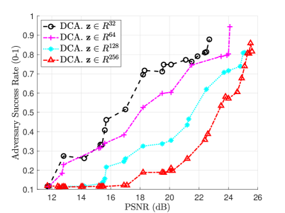
Figure 3: Privacy-utility trade-off of the MNIST dataset in different code length. Here, $\boldsymbol{x}\in\mathbb{R}^{784}$ whereas $\boldsymbol{z}\in\mathbb{R}^{d}$.

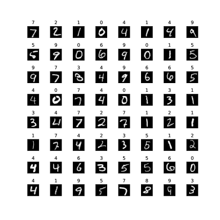
(a) Data Samples

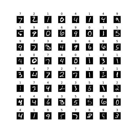
(b) Reconstruction (our DCA)

Figure 4: Testing data versus reconstruction from the DCA solver. PSNR=$24$ dB, Adversary success rate=$0.57$

In training the proposed neural networks prototype, we update the weights alternatingly. We fix the weights of the encoder and update the decoder with (16a). Then we fix the weights of the updated decoder and update the encoder parameters (including that of the prior) through (17a). This alternating procedure is implemented in PyTorch with the combination of an on/off requires_grad flag for the parameters of the encoder/decoder and activating the retain_graph flag in the backpropagation of (16a).

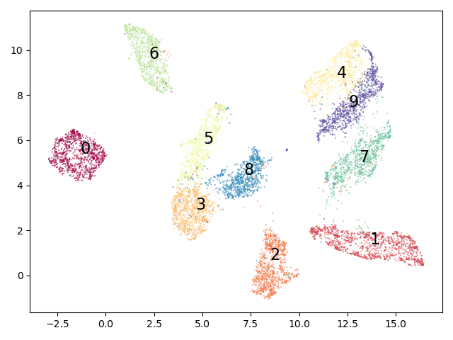
(a) Projection with $\boldsymbol{x}$ directly

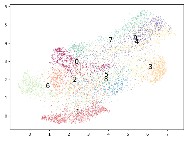
(b) Projection with our $\boldsymbol{z}$

Figure 5: Visualization of the codes from DCA solver. PSNR=$24$dB, Adversary success rate=$0.57$ and code length $d_{z}=256$. Centers of each class are labeled.

Appendix F Extended Evaluation: Compression Ratio and Privacy-Utility Trade-off

For the proposed approach, we further evaluate the relationship between the dimensionality of the compressed codes and the privacy-utility trade-off. Here, we focus on the MNIST dataset for its simplicity as shown in Section IV-B. Fig. 2a in the main content accounts for all $d_{z}\in\{32,64,128,256\}$, but here we separate each of the configurations to investigate its effects on the trade-off.

In Fig. 3, we show the adversary success rate versus the achieved PSNR of the proposed DCA solver with different configurations of the dimensionalty of $Z$, i.e., $d_{z}$. Our results show that the DCA solver can be more robust against privacy leakage (higher adversary success rate) with larger $d_{z}$. For MNIST dataset the number of dimensions of the public information $X$ is $d_{x}=784$ and since it is often desirable to find a compressed representation of $X$. Therefore, one can readily identify a computational trade-off in parallel to the privacy-utility trade-off. Specifically, a low compression ratio $d_{z}/d_{x}$ results in a low robustness against an adversary of the leakage of privacy $Y$ for a fixed reconstruction quality of the public information $X$. The characterization of the computation trade-off will be left for future work.

Appendix G Extended Evaluation: Visualization

In Fig. 4b, we show the first $64$ samples of the MNIST testing samples with the reconstruction of the proposed DCA solver with $\alpha=0.01$ and $\beta=0.05$. The PSNR for this configuration results is $24$ dB with adversarial success rate of $0.57$. The samples are perceptually recognizable after reconstruction, demonstrating sufficient utility of the images $X$. Then in Fig. 5b, we visualize the projected $Z$ of the same configuration. Moreover, we compare the $2$-dimensional projection from our code to direct projection of $X$, i.e., no privatization. As shown from Fig. 5b, projecting our privatized codes has more ambiguity between all classes whereas in Fig. 5a, the direct projection baseline reveals recognizable separation between them instead. This means lower privacy leakage for the proposed approach under sufficient reconstruction quality.

References

- [1] A. Makhdoumi, S. Salamatian, N. Fawaz, and M. Médard, “From the information bottleneck to the privacy funnel,” in 2014 IEEE Information Theory Workshop (ITW 2014), pp. 501–505, 2014.
- [2] T. M. Cover, Elements of information theory. John Wiley & Sons, 1999.
- [3] N. Ding and P. Sadeghi, “A submodularity-based clustering algorithm for the information bottleneck and privacy funnel,” in 2019 IEEE Information Theory Workshop (ITW), pp. 1–5, 2019.
- [4] T.-H. Huang, A. E. Gamal, and H. E. Gamal, “A linearly convergent Douglas-Rachford splitting solver for Markovian information-theoretic optimization problems,” IEEE Transactions on Information Theory, vol. 69, no. 5, pp. 3372–3399, 2023.
- [5] H. Attouch, J. Bolte, P. Redont, and A. Soubeyran, “Proximal alternating minimization and projection methods for nonconvex problems: An approach based on the Kurdyka-łojasiewicz inequality,” Mathematics of operations research, vol. 35, no. 2, pp. 438–457, 2010.
- [6] A. A. Alemi, I. Fischer, J. V. Dillon, and K. Murphy, “Deep variational information bottleneck,” arXiv preprint arXiv:1612.00410, 2016.
- [7] B. Rodríguez-Gálvez, R. Thobaben, and M. Skoglund, “A variational approach to privacy and fairness,” in 2021 IEEE Information Theory Workshop (ITW), pp. 1–6, IEEE, 2021.
- [8] B. Razeghi, P. Rahimi, and S. Marcel, “Deep variational privacy funnel: General modeling with applications in face recognition,” arXiv preprint arXiv:2401.14792, 2024.
- [9] H. A. Le Thi and T. Pham Dinh, “Dc programming and dca: thirty years of developments,” Mathematical Programming, vol. 169, no. 1, pp. 5–68, 2018.
- [10] F. P. Calmon, A. Makhdoumi, and M. Médard, “Fundamental limits of perfect privacy,” in 2015 IEEE International Symposium on Information Theory (ISIT), pp. 1796–1800, 2015.
- [11] C. Schieler and P. Cuff, “Rate-distortion theory for secrecy systems,” IEEE Transactions on Information Theory, vol. 60, no. 12, pp. 7584–7605, 2014.
- [12] K. Kittichokechai and G. Caire, “Privacy-constrained remote source coding,” in 2016 IEEE International Symposium on Information Theory (ISIT), pp. 1078–1082, 2016.
- [13] Y. Yakimenka, H.-Y. Lin, E. Rosnes, and J. Kliewer, “Optimal rate-distortion-leakage tradeoff for single-server information retrieval,” IEEE Journal on Selected Areas in Communications, vol. 40, no. 3, pp. 832–846, 2022.
- [14] Y. Y. Shkel, R. S. Blum, and H. V. Poor, “Secrecy by design with applications to privacy and compression,” IEEE Transactions on Information Theory, vol. 67, no. 2, pp. 824–843, 2021.
- [15] D. L. Donoho, “Compressed sensing,” IEEE Transactions on information theory, vol. 52, no. 4, pp. 1289–1306, 2006.
- [16] N. R. Draper and F. Pukelsheim, “Generalized ridge analysis under linear restrictions, with particular applications to mixture experiments problems,” Technometrics, vol. 44, no. 3, pp. 250–259, 2002.
- [17] B. R. Gaines, J. Kim, and H. Zhou, “Algorithms for fitting the constrained lasso,” Journal of Computational and Graphical Statistics, vol. 27, no. 4, pp. 861–871, 2018.
- [18] M. Pilanci, L. Ghaoui, and V. Chandrasekaran, “Recovery of sparse probability measures via convex programming,” Advances in Neural Information Processing Systems, vol. 25, 2012.
- [19] F. Pedregosa, G. Varoquaux, A. Gramfort, V. Michel, B. Thirion, O. Grisel, M. Blondel, P. Prettenhofer, R. Weiss, V. Dubourg, J. Vanderplas, A. Passos, D. Cournapeau, M. Brucher, M. Perrot, and E. Duchesnay, “Scikit-learn: Machine learning in Python,” Journal of Machine Learning Research, vol. 12, pp. 2825–2830, 2011.
- [20] D. P. Kingma and M. Welling, “Auto-encoding variational Bayes,” arXiv preprint arXiv:1312.6114, 2013.
- [21] J. Duchi, “Derivations for linear algebra and optimization,” Berkeley, California, vol. 3, no. 1, pp. 2325–5870, 2007.
- [22] Y. Park, C. Kim, and G. Kim, “Variational Laplace autoencoders,” in International conference on machine learning, pp. 5032–5041, PMLR, 2019.
- [23] T.-H. Huang, T. Dahanayaka, K. Thilakarathna, P. H. Leong, and H. El Gamal, “The Wyner variational autoencoder for unsupervised multi-layer wireless fingerprinting,” in GLOBECOM 2023 - 2023 IEEE Global Communications Conference, pp. 820–825, 2023.
- [24] S. Asoodeh and F. P. Calmon, “Bottleneck problems: An information and estimation-theoretic view,” Entropy, vol. 22, no. 11, p. 1325, 2020.
- [25] Y. LeCun, C. Cortes, and C. Burges, “Mnist handwritten digit database,” ATT Labs [Online]. Available: http://yann.lecun.com/exdb/mnist, vol. 2, 2010.
- [26] H. Xiao, K. Rasul, and R. Vollgraf, “Fashion-mnist: a novel image dataset for benchmarking machine learning algorithms,” arXiv preprint arXiv:1708.07747, 2017.
- [27] L. McInnes, J. Healy, and J. Melville, “Umap: Uniform manifold approximation and projection for dimension reduction,” arXiv preprint arXiv:1802.03426, 2018.
- [28] D. P. Kingma and J. Ba, “ADAM: A method for stochastic optimization,” arXiv preprint arXiv:1412.6980, 2014.
- [29] T.-H. Huang and H. El Gamal, “Efficient alternating minimization solvers for Wyner multi-view unsupervised learning,” in 2023 IEEE International Symposium on Information Theory (ISIT), pp. 707–712, 2023.
- [30] T.-H. Huang and H. E. Gamal, “Efficient solvers for Wyner common information with application to multi-modal clustering,” arXiv preprint arXiv:2402.14266, 2024.
- [31] A. Radford, L. Metz, and S. Chintala, “Unsupervised representation learning with deep convolutional generative adversarial networks,” arXiv preprint arXiv:1511.06434, 2015.