Extensive-Form Game Solving via Blackwell Approachability on Treeplexes

Abstract

In this paper, we introduce the first algorithmic framework for Blackwell approachability on the sequence-form polytope, the class of convex polytopes capturing the strategies of players in extensive-form games (EFGs). This leads to a new class of regret-minimization algorithms that are stepsize-invariant, in the same sense as the regret matching and regret matching⁺ algorithms for the simplex. Our modular framework can be combined with any existing regret minimizer over cones to compute a Nash equilibrium in two-player zero-sum EFGs with perfect recall, through the self-play framework. Leveraging predictive online mirror descent, we introduce Predictive Treeplex Blackwell⁺ (PTB⁺), and show a $O(1/\sqrt{T})$ convergence rate to Nash equilibrium in self-play. We then show how to stabilize PTB⁺ with a stepsize, resulting in an algorithm with a state-of-the-art $O(1/T)$ convergence rate. We provide an extensive set of experiments to compare our framework with several algorithmic benchmarks, including CFR⁺ and its predictive variant, and we highlight interesting connections between practical performance and the stepsize-dependence or stepsize-invariance properties of classical algorithms.

1 Introduction

In this paper, we focus on solving Extensive-Form Games (EFGs), a widely used framework for modeling repeated games with perfect or imperfect information. Finding a Nash equilibrium of a two-player zero-sum EFG can be cast as solving a saddle-point problem of the form

$$\min_{\bm{x}\in\mathcal{X}}\max_{\bm{y}\in\mathcal{Y}}\;\langle\bm{x},\bm{M}\bm{y}\rangle$$ (1.1)

where the sets $\mathcal{X},\mathcal{Y}$ are two sequence-form polytopes (also referred to as treeplexes) representing the strategies $\bm{x},\bm{y}$ of each player, and $\bm{M}$ is a payoff matrix. EFGs have been successfully used to obtain superhuman performances in several recent poker AI breakthroughs (Tammelin et al., 2015; Brown and Sandholm, 2018, 2019).

Many algorithms have been developed based on (1.1). Since $\mathcal{X}$ and $\mathcal{Y}$ are polytopes, (1.1) can be formulated as a linear program (von Stengel, 1996). However, because $\mathcal{X}$ and $\mathcal{Y}$ themselves have very large dimensions in realistic applications, first-order methods (FOMs) and regret minimization approaches are preferred for large-scale game solving. FOMs such as the Excessive Gap Technique (EGT, Nesterov (2005)) and Mirror Prox (Nemirovski, 2004) instantiated for EFGs (Hoda et al., 2010; Kroer et al., 2020) converge to a Nash equilibrium at a rate of $O(1/T)$, where $T$ is the number of iterations. Regret minimization techniques rely on a folk theorem relating the regrets of the players and the duality gap of the average iterates (Freund and Schapire, 1999). For instance, predictive online mirror descent with with the treeplexes $\mathcal{X}$ and $\mathcal{Y}$ as decision sets achieves a $O(1/T)$ convergence rate Farina et al. (2019b).

Counterfactual regret minimization (CFR) Zinkevich et al. (2007) is a regret minimizer for the treeplex that runs regret minimizers locally, i.e. directly at the level of the information sets of each player. In particular, CFR⁺, used in virtually all poker AI milestones Tammelin et al. (2015); Moravčík et al. (2017); Brown and Sandholm (2019), instantiates the CFR framework with a regret minimizer called Regret Matching⁺ (RM⁺) Tammelin et al. (2015) and guarantees a $O(1/\sqrt{T})$ convergence rate. The strong empirical performance of CFR⁺ remains mostly unexplained, since this algorithm does not achieve the fastest theoretical $O(1/T)$ convergence rate. Interestingly, there is a stark contrast between the role of stepsizes in CFR⁺ versus in other algorithms. CFR⁺ may use different stepsizes across different infosets, and the iterates of CFR⁺ do not depend on the values of these stepsizes. We identify this property as infoset stepsize invariance. In contrast, the convergence properties of FOMs depend on the choice of a single stepsize used across the entire treeplex, which may be hard to tune in practice.

RM⁺ arises as an instantiation of Blackwell approachability Blackwell (1956) for the simplex. Blackwell approachability is a versatile framework with connections to online learning Abernethy et al. (2011) and applications in stochastic games Milman (2006), calibration Perchet (2010) and revenue management Niazadeh et al. (2021). Empirically, combining CFR with other local regret minimizers than RM⁺, e.g. Online Mirror Descent (OMD), does not lead to the strong practical performance as CFR⁺ Brown et al. (2017). This suggests that using a regret minimizer based on Blackwell approachability (RM⁺) is central to the success of CFR⁺.

Our goal is to develop Blackwell approachability-based algorithms for treeplexes. Our contributions are as follows.

Treeplex Blackwell approachability. We introduce the first Blackwell approachability-based regret minimizer for treeplexes. Using the self-play framework, we correspondingly get the first framework for solving two-player zero-sum EFGs via Blackwell approachability on treeplexes. Blackwell approachability enables an equivalence between regret minimization over the treeplex $\mathcal{T}$ and regret minimization over its conic hull ${\sf cone}(\mathcal{T})$, and any existing regret minimizer for ${\sf cone}(\mathcal{T})$ yields a new algorithm for solving EFGs. A crucial advantage of using Blackwell approachability on the treeplex, rather than regret minimization directly on the treeplex, is that it leads to a variety of interesting stepsize properties (e.g. stepsize invariance), which are not achieved by regret minimizers such as OMD on the treeplex. We instantiate our framework with several regret minimizers, leading to different desirable properties.

PTB⁺ (Predictive Treeplex Blackwell⁺, Algorithm 2) combines our framework with predictive online mirror descent over ${\sf cone}(\mathcal{T})$ and achieves a $O(1/\sqrt{T})$ convergence rate. As an instantiation of Blackwell approachability over a cone, PTB⁺ is treeplex stepsize invariant, i.e., its iterates do not change if we rescale all stepsizes by a positive constant. This is a desirable property for practical use, although it is a weaker property than the infoset stepsize invariance of CFR⁺.

Smooth PTB⁺ (Algorithm 3) is a variant of PTB⁺ ensuring that successive iterates vary smoothly. This stability is a central element of the fastest algorithms for EFGs and we show that Smooth PTB⁺ has a $O(1/T)$ convergence rate. Smooth PTB⁺ is the first EFG-solving algorithm based on Blackwell approachability achieving the state-of-the-art theoretical convergence rate, answering an important open question.

AdaGradTB⁺(Algorithm 4) combines our framework with AdaGrad Duchi et al. (2011) as a regret minimizer over ${\sf cone}(\mathcal{T})$. AdaGradTB⁺ adaptively learns different stepsizes for every dimension of the treeplexes and guarantees a $O(1/\sqrt{T})$ convergence rate. For completeness, we consider AdamTB⁺, an adaptive instantiation of our framework based on Adam Kingma and Ba (2015), a widely used algorithm lacking regret guarantees.

The convergence properties of our algorithms compared to existing methods can be found in Table 1.

Numerical experiments. We provide two comprehensive sets of numerical experiments over benchmark EFGs.

We first compare the performance of all the algorithms introduced in our paper (Figure 4) and find that PTB⁺ performs the best. This highlights the advantage of treeplex stepsize invariant algorithms (PTB⁺) over stepsize-dependent algorithms, even ones achieving faster theoretical convergence rate (Smooth PTB⁺), and over adaptive algorithms learning decreasing stepsizes (AdaGradTB⁺). AdamTB⁺ diverge on some instances, since Adam is not a regret minimizer.

We then compare our best method (PTB⁺) with several existing algorithms for EFGs: CFR⁺, its predictive variants (PCFR⁺), and predictive OMD (POMD) (Figure 2). We find that PCFR⁺ outperforms all other algorithms in terms of average-iterate performance. This suggests that infoset stepsize invariance is an important property, moreso than the treeplex stepsize invariance of PTB⁺. Because of the CFR decomposition, PCFR⁺ can use different stepsizes at different infosets, where the values of the variables may be of very different magnitudes (typically, smaller for infosets appearing deeper in the treeplex), and PCFR⁺ does not require tuning these different stepsizes, which may be impossible for large instances. As part of our main contributions, we identify and distinguish the infoset stepsize invariance and treeplex stepsize invariance properties; based on our empirical experiments, we posit that part of the puzzle behind the strong empirical performances of CFR⁺ and PCFR⁺ can be explained by the infoset stepsize invariance property. We also compare the last-iterate performances, where no algorithms appear to consistently outperform the others. We leave studying the last-iterate convergence as an open question.

Algorithms	Convergence rate	Stepsize invariance
CFR+ Tammelin et al. (2015)	$1/\sqrt{T}$	$\checkmark\checkmark$
PCFR+ Farina et al. (2021b)	$1/\sqrt{T}$	$\checkmark\checkmark$
EGT Kroer et al. (2018)	$1/T$	✗
POMD Farina et al. (2019b)	$1/T$	✗
PTB+ (Algorithm 2)	$1/\sqrt{T}$	$\checkmark$
Smooth PTB+ (Algorithm 3)	$1/T$	✗
AdaGradTB+ (Algorithm 4)	$1/\sqrt{T}$	✗
AdamTB+ (Algorithm 7)	$?$	✗

Table 1: Convergence rates to a Nash equilibrium of a two-player zero-sum EFG for several algorithms. $\checkmark\checkmark$ refers to infoset stepsize invariance and $\checkmark$ refers to treeplex stepsize invariance.

2 Preliminaries on EFGs

We first provide some background on EFGs and treeplexes.

Extensive-form games.

Two-player zero-sum extensive-form games (later referred to as EFGs) are represented by a game tree and a payoff matrix. Each node of the tree belongs either to the first player, to the second player, or to a chance player, modeling the random events that happen in the game, e.g., tossing a coin. The players are assigned payoffs at the terminal nodes only. Imperfect/private information is modeled using information sets (later referred to as infosets), which are subsets of nodes of the game tree. A player cannot distinguish between the nodes in a given infoset, and they must take the same action at all these nodes.

Treeplexes.

The strategy of a player can be described by a polytope called the treeplex, also known as the sequence-form polytope. The treeplex is constructed as follows. We index the infosets of a player by $\mathcal{J}=\{1,...,|\mathcal{J}|\}$. The set of actions available at infoset $j\in\mathcal{J}$ is written $\mathcal{A}_{j}$ with cardinality $|\mathcal{A}_{j}|=n_{j}$. We represent choosing action $a\in\mathcal{A}_{j}$ at infoset $j\in\mathcal{J}$ by a sequence $(j,a)$, and we denote by $\mathcal{C}_{ja}$ the set of next infosets reachable from $(j,a)$ (possibly empty if the game terminates). The parent $p_{j}$ of an infoset $j\in\mathcal{J}$ is the sequence leading to $j$; note that $p_{j}$ is unique assuming perfect recall. We assume that there is a single root denoted as $\varnothing$ and called the empty sequence. If the player does not take any action before reaching $j\in\mathcal{J}$, then by convention $p_{j}=\varnothing$. Under the perfect recall assumption, the set of infosets has a tree structure: $\mathcal{C}_{ja}\cap\mathcal{C}_{j^{\prime}a^{\prime}}=\emptyset$, for all pairs of sequences $(j,a)$ and $(j^{\prime},a^{\prime})$ such that $j\neq j^{\prime},a\neq a^{\prime}$. This tree is the treeplex and it represents the set of all admissible strategies for a given player. We denote by $n\in\mathbb{N}$ the total number of sequences $(j,a)$ with $j\in\mathcal{J}$ and $a\in\mathcal{A}_{j}$. With these notations, the treeplex $\mathcal{T}$ of a given player can be written as

$$\mathcal{T}=\{\bm{x}\in\mathbb{R}^{n+1}_{+}\;|\;x_{\varnothing}=1,\sum_{a\in\mathcal{A}_{j}}x_{ja}=x_{p_{j}},\forall\;j\in\mathcal{J}\}$$ (2.1)

where the first component $x_{\varnothing}$ is related to the empty sequence $\varnothing$. We say that a player makes an observation to arrive at $j$, if $|\mathcal{C}_{p_{j}}|>1$. We define the depth $d$ of a treeplex to be the maximum number of actions and observations that can be made starting at the root until reaching a leaf infoset. Computing a Nash equilibrium of EFGs can be formulated as solving (1.1) (under the perfect recall assumption), with $\mathcal{X}\subset\mathbb{R}^{n_{1}+1}$ and $\mathcal{Y}\subset\mathbb{R}^{n_{2}+1}$ the treeplex of each player, $n_{1}$ and $n_{2}$ are the number of sequences of each player, and $\bm{M}\in\mathbb{R}^{(n_{1}+1)\times(n_{2}+1)}$ the payoff matrix such that for a pair of strategy $(\bm{x},\bm{y})\in\mathcal{X}\times\mathcal{Y}$, $\langle\bm{x},\bm{M}\bm{y}\rangle$ is the expected value that the second player receives from the first player.

Regret minimization and self-play framework.

A regret minimizer Regmin over a decision set $\mathcal{Z}\subset\mathbb{R}^{d}$ is an algorithm such that, at every iteration, Regmin chooses a decision $\bm{z}^{t}\in\mathcal{Z}$, a loss vector $\bm{\ell}\in\mathbb{R}^{d}$ is observed, and the scalar loss $\langle\bm{\ell}^{t},\bm{x}^{t}\rangle$ is incurred. A regret minimizer ensures that the regret ${\sf Reg}^{T}=\max_{\hat{\bm{z}}\in\mathcal{Z}}\sum_{t=1}^{T}\langle\bm{\ell}^{t},\bm{z}^{t}-\hat{\bm{z}}\rangle$ grows at most as $O(\sqrt{T})$. As an example, predictive online mirror descent (POMD, Rakhlin and Sridharan (2013)) generates a sequence of decisions $\bm{z}_{1},...,\bm{z}_{T}\in\mathcal{Z}$ as follows:

$$\bm{z}_{t} =\Pi_{\mathcal{Z}}\left(\hat{\bm{z}}_{t}-\eta\bm{m}_{t}\right)$$ (2.2)

$$\hat{\bm{z}}_{t+1} =\Pi_{\mathcal{Z}}\left(\hat{\bm{z}}_{t}-\eta\bm{\ell}_{t}\right)$$

with $\bm{m}_{1},...,\bm{m}_{T}\in\mathbb{R}^{d}$ some predictions of the losses $\bm{\ell}_{1},...,\bm{\ell}_{T}\in\mathbb{R}^{d}$, and where we write the orthogonal projection of $\bm{y}\in\mathbb{R}^{d}$ onto $\mathcal{Z}$ as $\Pi_{\mathcal{Z}}\left(\bm{y}\right):=\arg\min_{\bm{z}\in\mathcal{Z}}\|\bm{z}-\bm{y}\|_{2}$.

The self-play framework leverages regret minimization to solve EFGs. The players compute two sequences of strategies $\bm{x}_{1},...,\bm{x}_{T}$ and $\bm{y}_{1},...,\bm{y}_{T}$ such that, at iteration $t\geq 1$, the first player observes its loss vector $\bm{A}\bm{y}_{t-1}$ and the second player observes its loss vector $-\bm{A}^{\top}\bm{x}_{t-1}$. Each player computes their current strategies $\bm{x}_{t}\in\mathcal{X}$ and $\bm{y}_{t}\in\mathcal{Y}$ by using a regret minimizer. A well-known folk theorem states that the duality gap of the average of the iterates is bounded by the sum of the average regrets of the players.

Proposition 2.1 ((Freund and Schapire, 1999)).

Let $\bm{x}_{1},...,\bm{x}_{T}\in\mathcal{X}$ and $\bm{y}_{1},...,\bm{y}_{T}\in\mathcal{Y}$ be computed in the self-play framework. Let $\left(\bar{\bm{x}}_{T},\bar{\bm{y}}_{T}\right)=\frac{1}{T}\sum_{t=1}^{T}\left(\bm{x}_{t},\bm{y}_{t}\right)$. Then, for ${\sf Reg}^{T}_{1}$ and ${\sf Reg}^{T}_{2}$ the regret of each player,

$$\max_{\hat{\bm{y}}\in\mathcal{Y}}\;\langle\bar{\bm{x}}_{T},\bm{M}\hat{\bm{y}}\rangle-\min_{\hat{\bm{x}}\in\mathcal{X}}\;\langle\hat{\bm{x}},\bm{M}\bar{\bm{y}}_{T}\rangle=\frac{{\sf Reg}^{T}_{1}+{\sf Reg}^{T}_{2}}{T}.$$

We present more details on the self-play framework in Appendix A. Several regret minimizers exist for the treeplex, e.g. POMD (Farina et al., 2021a).

CFR and Regret Matching⁺.

Counterfactual Regret minimization (CFR, Zinkevich et al. (2007)) runs independent regret minimizers with counterfactual losses at each infoset of the treeplexes. This considerably simplifies the optimization problem, since the decision set at each infoset $j\in\mathcal{J}$ is the simplex over the set of next available actions $\Delta^{n_{j}}:=\{\bm{x}\in\mathbb{R}_{+}^{n_{j}}\;|\;\sum_{i=1}^{n_{j}}x_{i}=1\}$. In the CFR framework, the regret of each player (over the treeplex) is bounded by the maximum of the local regrets incurred at each infoset. Therefore, CFR combined with any regret minimizer over the simplex converges to a Nash equilibrium at a rate of $O(1/\sqrt{T})$. We refer to Appendix B for more details. Combining CFR with a local regret minimizer called Regret Matching⁺ (RM⁺, Tammelin et al. (2015)) along with alternation and linear averaging yields an algorithm called CFR⁺, which has been observed to attain strong practical performance compared to theoretically-faster methods (Kroer et al., 2020). RM⁺ can only be implemented on the simplex and not for other decision sets, and proceeds as follows: given a sequence of loss $\bm{\ell}_{1},...,\bm{\ell}_{T}\in\mathbb{R}^{d}$, RM⁺ maintains a sequence $\bm{R}_{1},...,\bm{R}_{T}\in\mathbb{R}^{d}$ such that $\bm{R}_{1}=\bm{0}$ and

$$\bm{x}_{t} =\bm{R}_{t}/\|\bm{R}_{t}\|_{1},\bm{R}_{t+1}=\Pi_{\mathbb{R}_{+}^{d}}\left(\bm{R}_{t}-\eta\bm{g}(\bm{x}_{t},\bm{\ell}_{t})\right)$$ (2.3)

with $\eta>0$ and, for $\bm{x},\bm{\ell}\in\mathbb{R}^{d}$,

$$\bm{g}(\bm{x},\bm{\ell}) :=\bm{\ell}-\langle\bm{x},\bm{\ell}\rangle\bm{1}.$$ (2.4)

We use the convention $\bm{0}/0:=(1/d)\bm{1}$ with $\bm{1}:=(1,...,1)\in\mathbb{R}^{d}$. RM⁺ is stepsize invariant: $\bm{x}_{1},...,\bm{x}_{T}$ are independent of $\eta$, since we have $\bm{x}_{t}=\bm{R}_{t}/\|\bm{R}_{t}\|_{1}$ and $\eta$ only rescales the entire sequence $\bm{R}_{1},...,\bm{R}_{T}$. Since CFR⁺ runs RM⁺ at each infoset independently, CFR⁺ is infoset stepsize invariant: there may be different stepsizes across different infosets and the iterates of CFR⁺ do not depend on their values, a desirable property when solving large-scale EFGs where stepsize tuning may be difficult.

RM⁺ can be interpreted as a special instantiation of Blackwell approachability (Blackwell, 1956; Abernethy et al., 2011). In this interpretation of RM⁺, the goal of the decision maker is to compute the sequence of strategies $\bm{x}_{1},...,\bm{x}_{T}\in\Delta^{d}$ to ensure that the auxiliary sequence $\bm{R}_{T}/T\in\mathbb{R}_{+}^{d}$ approaches the target set $\mathbb{R}_{-}^{d}$ as $T\rightarrow+\infty$. Since $\bm{R}_{t}\in\mathbb{R}_{+}^{d}$, this is equivalent to ensuring that $\lim_{T\rightarrow+\infty}\bm{R}_{T}/T=\bm{0}$. The vector $\bm{g}(\bm{x},\bm{\ell})$ is interpreted as an instantaneous loss for the approachability instance. As an instantiation of Blackwell approachability, at each iteration RM⁺ computes an orthogonal projection onto the conic hull of the decision set:

$$\mathbb{R}_{+}^{d}={\sf cone}(\Delta^{d})$$ (2.5)

with ${\sf cone}(\mathcal{Z}):=\{\alpha\bm{x}\;|\;\bm{x}\in\mathcal{Z},\alpha\geq 0\}$ for a set $\mathcal{Z}$. The decision function $\bm{R}\mapsto\bm{R}/\|\bm{R}\|_{1}$ is based on

$$\Delta^{d}\subset\{\bm{x}\in\mathbb{R}^{d}\;|\;\langle\bm{x},\bm{1}\rangle=1\}.$$ (2.6)

Since for $\bm{R}\in\mathbb{R}_{+}^{d},\langle\bm{R},\bm{1}\rangle=\|\bm{R}\|_{1}$, then $\bm{x}_{t}=\bm{R}_{t}/\|\bm{R}_{t}\|_{1}$ can be written $\bm{x}_{t}=\bm{R}_{t}/\langle\bm{R}_{t},\bm{1}\rangle$, with $\bm{1}$ a vector such that the decision set $\Delta^{d}$ satisfies (2.6). This ensures that

$$\langle\bm{R}_{t},\bm{g}(\bm{x}_{t},\bm{\ell})\rangle=0,\forall\;\bm{\ell}\in\mathbb{R}^{d}.$$ (2.7)

We provide an illustration of the dynamics of RM⁺ in Figure 1. Equation (2.7) is known as a hyperplane forcing condition and is a key ingredient in any Blackwell approachability-based algorithm; it ensures that the vector $\bm{R}_{T}$ grows at most at a rate of $O(\sqrt{T})$ so that $\lim_{T\rightarrow+\infty}\bm{R}_{T}/T=\bm{0}$. We refer to Perchet (2010); Grand-Clément and Kroer (2023) for more details on Blackwell approachability.

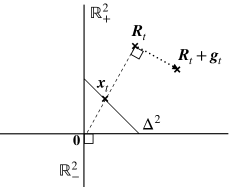
Figure 1: Dynamics of RM⁺ in $\mathbb{R}_{+}^{2}$. We write $\bm{g}_{t}=\bm{g}(\bm{x}_{t},\bm{\ell}_{t})$.

3 Blackwell Approachability on Treeplexes

In this section we introduce a modular regret minimization framework for the treeplex based on Blackwell approachability. This framework can be used as a regret minimizer over $\mathcal{T}$ in the self-play framework (described in the previous section and in Appendix A) to obtain an algorithm for solving EFGs. Our algorithms are based on the fact that for $\mathcal{T}\subset\mathbb{R}^{n+1}$ a treeplex as defined in (2.1), we have

$$\mathcal{T}\subset\{\bm{x}\in\mathbb{R}^{n+1}\;|\;\langle\bm{x},\bm{a}\rangle=1\}$$ (3.1)

for $\bm{a}=(1,\bm{0})\in\mathbb{R}^{n+1}$ with $\bm{0}=(0,...,0)\in\mathbb{R}^{n}$. This property is analogous to (2.6) for the simplex. With this analogy in mind, we define $\mathcal{C}\subset\mathbb{R}^{n+1}$ and $\bm{f}(\bm{x},\bm{\ell})\in\mathbb{R}^{n+1}$ as, for $\bm{x},\bm{\ell}\in\mathbb{R}^{n+1}$,

$$\mathcal{C} :={\sf cone}(\mathcal{T})$$ (3.2)

$$\bm{f}(\bm{x},\bm{\ell}) :=\bm{\ell}-\langle\bm{x},\bm{\ell}\rangle\bm{a}.$$ (3.3)

Equation (3.2) is analogous to (2.5) and Equation (3.3) is analogous to (2.4). The cone $\mathcal{C}$ and the vector $\bm{f}(\bm{x},\bm{\ell})$ play a similar role for $\mathcal{T}$ as $\mathbb{R}_{+}^{d}$ and $\bm{g}(\bm{x},\bm{\ell})$ play for $\Delta^{d}$ in RM⁺.

Our Blackwell approachability-based framework is described in Algorithm 1 and relies on running a regret minimizer Regmin over $\mathcal{C}={\sf cone}(\mathcal{T})$ against the losses $\bm{f}(\bm{x}_{t},\bm{\ell}_{t})$ to obtain a regret minimizer over $\mathcal{T}$ against the losses $\bm{\ell}_{t}$, for $t\geq 1$.

Algorithm 1 Blackwell approachability on the treeplex

1:Input: A regret minimizer ${\sf Regmin}$ with decision set $\mathcal{C}$

2:Initialization: $\bm{R}_{1}=\bm{0}\in\mathbb{R}^{n+1}$

3:for $t=1,\dots,T$ do

4:     $\bm{x}_{t}=\bm{R}_{t}/\langle\bm{R}_{t},\bm{a}\rangle$

5:     Observe the loss vector $\bm{\ell}_{t}\in\mathbb{R}^{n+1}$

6:     Regmin observes $\bm{f}(\bm{x}_{t},\bm{\ell}_{t})\in\mathbb{R}^{n+1}$

7:     $\bm{R}_{t+1}={\sf Regmin}\left(\cdot\right)$

We use the convention that $\bm{0}/0$ is the uniform strategy for the treeplex. Algorithm 1 is the first Blackwell approachability-based algorithm operating on the entire treeplex (in contrast to CFR⁺ which relies on Blackwell approachability locally at the infosets level). We first describe some important properties of Algorithm 1:

Feasibility of the current iterate. Algorithm 1 produces a feasible sequence of strategies, i.e., $\bm{x}_{t}\in\mathcal{T},\forall\;t\geq 1$. Indeed, since Regmin is a regret minimizer with $\mathcal{C}$ as the decision set, $\bm{R}_{t}\in{\sf cone}(\mathcal{T})$, i.e., $\bm{R}_{t}=\alpha\bm{z}$ with $\alpha\in\mathbb{R}_{+}$ and $\bm{z}\in\mathcal{T}$. From (3.1), we have $\langle\bm{z},\bm{a}\rangle=1$. Therefore, $\bm{x}_{t}=\frac{\bm{R}_{t}}{\langle\bm{R}_{t},\bm{a}\rangle}=\frac{\alpha\bm{z}}{\alpha\langle\bm{z},\bm{a}\rangle}=\bm{z}\in\mathcal{T}.$ This is analogous to RM⁺, where $\bm{x}_{t}$ is proportional to $\bm{R}_{t}$, see (2.3) and Figure 1.

Hyperplane forcing. For any $t\in\mathbb{N}$ we have

$$\langle\bm{R}_{t},f(\bm{x}_{t},\bm{\ell})\rangle=0,\forall\;\bm{\ell}\in\mathbb{R}^{n+1}.$$ (3.4)

The hyperplane forcing equation (3.4) is a crucial component of algorithms based on Blackwell approachability. It ensures that $\|\bm{R}_{t}\|_{2}=O(\sqrt{T})$. Equation (3.4) is analogous to (2.7) for RM⁺ and follows from $\bm{x}_{t}=\frac{\bm{R}_{t}}{\langle\bm{R}_{t},\bm{a}\rangle}$, so that

$$\langle\bm{R}_{t},\bm{f}(\bm{x}_{t},\bm{\ell})\rangle =\langle\bm{R}_{t},\bm{\ell}\rangle-\langle\bm{x}_{t},\bm{\ell}\rangle\langle\bm{R}_{t},\bm{a}\rangle$$

$$=\langle\bm{R}_{t},\bm{\ell}\rangle-\langle\frac{\bm{R}_{t}}{\langle\bm{R}_{t},\bm{a}\rangle},\bm{\ell}\rangle\langle\bm{R}_{t},\bm{a}\rangle$$

$$=\langle\bm{R}_{t},\bm{\ell}\rangle-\langle\bm{R}_{t},\bm{\ell}\rangle=0.$$

Regret minimization over $\mathcal{T}$. Crucially, Algorithm 1 always yields a regret minimizer over the treeplex $\mathcal{T}$, i.e., it ensures that the regret of $\bm{x}_{1},...,\bm{x}_{T}\in\mathcal{T}$ against any the sequence $\bm{\ell}_{1},...,\bm{\ell}_{T}\in\mathbb{R}^{n+1}$ is bounded by $O(\sqrt{T})$. The proof is instructive and shows a central component to Blackwell approachability-based algorithms: minimizing regret over $\mathcal{T}$ can be achieved by minimizing regret over ${\sf cone}(\mathcal{T})$.

Proposition 3.1.

Let ${\sf Regmin}$ be a regret minimizer with $\mathcal{C}$ as the decision set. Let $\bm{x}_{1},...,\bm{x}_{T}\in\mathcal{T}$ be computed by Algorithm 1. Then $\max_{\hat{\bm{x}}\in\mathcal{T}}\sum_{t=1}^{T}\langle\bm{x}_{t}-\hat{\bm{x}},\bm{\ell}_{t}\rangle=O(\sqrt{T}).$

Proof.

Let $\hat{\bm{x}}\in\mathcal{T}$ and let us write $\hat{\bm{R}}=\hat{\bm{x}}$. We have

$$\sum_{t=1}^{T}\langle\bm{x}_{t}-\hat{\bm{x}},\bm{\ell}_{t}\rangle =\sum_{t=1}^{T}\langle-\hat{\bm{x}},\bm{f}\left(\bm{x}_{t},\bm{\ell}_{t}\right)\rangle$$

$$=\sum_{t=1}^{T}\langle-\hat{\bm{R}},\bm{f}\left(\bm{x}_{t},\bm{\ell}_{t}\right)\rangle$$

$$=\sum_{t=1}^{T}\langle\bm{R}_{t}-\hat{\bm{R}},\bm{f}\left(\bm{x}_{t},\bm{\ell}_{t}\right)\rangle$$

where the first equality follows from the definition of $\bm{f}\left(\bm{x}_{t},\bm{\ell}_{t}\right)$ as in (3.3) and $\langle\bm{z},\bm{a}\rangle=1$ for any $\bm{z}\in\mathcal{T}$, the second equality is because $\hat{\bm{x}}=\hat{\bm{R}}$, and the last equality follows from the hyperplane forcing condition (3.4). Now note that $\sum_{t=1}^{T}\langle\bm{R}_{t}-\hat{\bm{R}},\bm{f}\left(\bm{x}_{t},\bm{\ell}_{t}\right)\rangle$ is the regret of a regret minimizer Regmin choosing $\bm{R}_{1},...,\bm{R}_{T}$ in the decision set $\mathcal{C}:={\sf cone}(\mathcal{T})$ against a sequence of loss $\bm{f}\left(\bm{x}_{1},\bm{\ell}_{1}\right),...,\bm{f}\left(\bm{x}_{T},\bm{\ell}_{T}\right)$ and a comparator $\hat{\bm{R}}\in{\sf cone}(\mathcal{T})$. Therefore, $\sum_{t=1}^{T}\langle\bm{R}_{t}-\hat{\bm{R}},\bm{f}\left(\bm{x}_{t},\bm{\ell}_{t}\right)\rangle=O(\sqrt{T})$. ∎

Remark 3.2 (Comparison with Lagrangian Hedging).

Algorithm 1 is related to Lagrangian Hedging (Gordon, 2007; D’Orazio and Huang, 2021). Lagrangian Hedging builds upon Blackwell approachability with various potential functions to construct regret minimizers for general decision sets. As explained in the introduction, the main focus of our paper is on two-player zero-sum EFGs, i.e., on the case where the decision sets are treeplexes, and where we can obtain several additional interesting properties not studied in (Gordon, 2007; D’Orazio and Huang, 2021), such as stepsize invariance, fast convergence rates, and efficient projection, as we detail in the next section. If one were to instantiate Algorithm 1 with the Follow-The-Regularized Leader algorithm, it would yield the regret minimizer for treeplexes studied in Gordon (2007), and our Proposition 4.4 yields an efficient projection oracle for the setup in Gordon (2007), which appealed to general convex optimization as an oracle.

4 Instantiations of Algorithm 1

We can instantiate Algorithm 1 with any regret minimizer over $\mathcal{C}$ to obtain various properties for the resulting algorithm, such as stepsize invariance, adaptive stepsizes, or achieving the state-of-the-art $O(1/T)$ convergence rate. We show next how to do so.

Predictive Treeplex Blackwell⁺ (PTB⁺).

We first introduce Predictive Treeplex Blackwell⁺ (Algorithm 2), combining Algorithm 1 with POMD with $\mathcal{C}$ as a decision set.

Algorithm 2 Predictive Treeplex Blackwell⁺(PTB⁺)

1:Input: $\eta>0$, predictions $\bm{m}_{1},...,\bm{m}_{T}\in\mathbb{R}^{n+1}$

2:Initialization: $\hat{\bm{R}}_{1}=\bm{0}\in\mathbb{R}^{n+1}$

3:for $t=1,\dots,T$ do

4:     $\bm{R}_{t}\in\Pi_{\mathcal{C}}\left(\hat{\bm{R}}_{t}-\eta\bm{m}_{t}\right)$

5:     $\bm{x}_{t}=\bm{R}_{t}/\langle\bm{R}_{t},\bm{a}\rangle$

6:     Observe the loss vector $\bm{\ell}_{t}\in\mathbb{R}^{n+1}$

7:     $\hat{\bm{R}}_{t+1}\in\Pi_{\mathcal{C}}\left(\hat{\bm{R}}_{t}-\eta\bm{f}(\bm{x}_{t},\bm{\ell}_{t})\right)$

We start by highlighting a crucial property of PTB⁺, treeplex stepsize invariance. The sequence of iterates $\bm{x}_{1},...,\bm{x}_{T}$ generated by Algorithm 2 is independent of the choice of the stepsize $\eta>0$, that only rescales the sequences $\hat{\bm{R}}_{1},...,\hat{\bm{R}}_{T}$ and $\bm{R}_{1},...,\bm{R}_{T}$, the orthogonal projection onto a cone is positively homogeneous of degree $1$: $\Pi_{\mathcal{C}}(\eta\bm{z})=\eta\Pi_{\mathcal{C}}(\bm{z})$ for $\eta>0$ and $\bm{z}\in\mathbb{R}^{n+1},$ and the function $\bm{R}\mapsto\bm{R}/\langle\bm{R},\bm{a}\rangle$ is scale-invariant: $\frac{(\eta\bm{R})}{\langle(\eta\bm{R}),\bm{a}\rangle}=\frac{\bm{R}}{\langle\bm{R},\bm{a}\rangle}$ for $\eta>0$ and $\bm{R}\in\mathbb{R}^{n+1}$. We provide a rigorous statement in the following proposition and we present the proof in Appendix C.

Proposition 4.1.

The sequence $\bm{x}_{1},...,\bm{x}_{T}$ computed by PTB⁺ after $T$ iterations is independent on the stepsize $\eta>0$.

Treeplex stepsize invariance is a crucial property, since in large EFGs, stepsize tuning is difficult and resource-consuming. This is the main advantage of using Blackwell approachability: running POMD directly on the treeplex $\mathcal{T}$ does not result in a stepsize invariant algorithm, whereas PTB⁺ runs POMD on ${\sf cone}(\mathcal{T})$ and is stepsize invariant. To our knowledge, CFR⁺ and PCFR⁺ are the only other treeplex stepsize invariant algorithms for solving EFGs. In fact, they satisfy a stronger infoset stepsize invariance property: different stepsizes can be used at different infosets, and the iterates do not depend on their values. We discuss the relation between PTB⁺ and known instantiations of Blackwell approachability over the simplex (RM⁺ and CBA⁺ Grand-Clément and Kroer (2023)) in Appendix D.

From Proposition 3.1 and the regret bounds on POMD (see for instance section 3.1.1 in Rakhlin and Sridharan (2013) or section 6 in Farina et al. (2021b)), we obtain the following proposition. We define $\Omega\in\mathbb{R}_{+}$ as $\Omega:=\max_{\bm{x}\in\mathcal{T}}\|\bm{x}\|_{2}.$

Proposition 4.2.

Let $\bm{x}_{1},...,\bm{x}_{T}$ be computed by PTB⁺. Then

$$\max_{\hat{\bm{x}}\in\mathcal{T}}\sum_{t=1}^{T}\langle\bm{x}_{t}-\hat{\bm{x}},\bm{\ell}_{t}\rangle\leq\Omega\sqrt{\sum_{t=1}^{T}\|\bm{f}(\bm{x}_{t},\bm{\ell}_{t})-\bm{m}_{t}\|_{2}^{2}}.$$

From Proposition 4.2, PTB⁺ is a regret minimizer over treeplexes, and we can combine it with the self-play framework to solve EFGs, as shown in the next corollary. We use the notations $d:=\max\{n,m\}+1,\hat{\Omega}:=\max\{\max\{\|\bm{x}\|_{2},\|\bm{y}\|_{2}\}\;|\;\bm{x}\in\mathcal{X},\bm{y}\in\mathcal{Y}\},\\ \|\bm{M}\|_{2}:=\sup\{\frac{\|\bm{Mv}\|_{2}}{\|\bm{v}\|_{2}}\;|\;\bm{v}\neq\bm{0}\}.$

Corollary 4.3.

Let $(\bm{x}_{t})_{t\geq 1}$ and $(\bm{y}_{t})_{t\geq 1}$ be the sequence of strategies computed by both players employing PTB⁺ in the self-play framework, with previous losses as predictions: $\bm{m}^{x}_{t}=\bm{f}(\bm{x}_{t-1},\bm{My}_{t-1}),\bm{m}^{y}_{t}=\bm{f}(\bm{y}_{t-1},-\bm{M}^{\top}\bm{x}_{t-1}).$ Let $\left(\bar{\bm{x}}_{T},\bar{\bm{y}}_{T}\right)=\frac{1}{T}\sum_{t=1}^{T}\left(\bm{x}_{t},\bm{y}_{t}\right)$. Then

$$\max_{\bm{y}\in\mathcal{Y}}\;\langle\bar{\bm{x}}_{T},\bm{My}\rangle-\min_{\bm{x}\in\mathcal{X}}\;\langle\bm{x},\bm{M}\bar{\bm{y}}_{T}\rangle\leq\frac{\hat{\Omega}^{3}\sqrt{d}\sqrt{\|\bm{M}\|_{2}}}{\sqrt{T}}.$$

Finally, we can efficiently compute the orthogonal projection onto $\mathcal{C}$ at every iteration to implement PTB⁺, since $\mathcal{C}$ admits the following simple formulation of as a polytope: $\mathcal{C}=\{\bm{x}\in\mathbb{R}^{n+1}_{+}\;|\;\sum_{a\in\mathcal{A}_{j}}x_{ja}=x_{p_{j}},\forall\;j\in\mathcal{J}\}.$

Proposition 4.4.

Let $\mathcal{T}$ be a treeplex with depth $d$, number of sequences $n$, number of leaf sequences $l$, and number of infosets $m$. The orthogonal projection $\Pi_{\mathcal{C}}(\bm{y})$ of a point $\bm{y}\in\mathbb{R}^{n+1}$ onto $\mathcal{C}={\sf cone}(\mathcal{T})$ can be computed in $O(dn\log(l+m))$ arithmetic operations.

A stable algorithm: Smooth PTB⁺.

We now modify PTB⁺ to obtain faster convergence rates for solving EFGs. The $O(1/\sqrt{T})$ average convergence rate of PTB⁺ may seem surprising since in the matrix game setting, POMD over the simplexes obtains a $O(1/T)$ average convergence (Syrgkanis et al., 2015). This discrepancy comes from PTB⁺ running POMD on the set $\mathcal{C}={\sf cone}(\mathcal{T})$ instead of the original decision set $\mathcal{T}$, so that the Lipschtiz continuity of the loss function and the classical RVU bounds (Regret Bounded by Variation in Utilities, see Equation (1) in Syrgkanis et al. (2015)), central to proving the fast convergence of predictive algorithms, may not hold. For PTB⁺, the Lipschitz continuity of the loss $\bm{R}\mapsto\bm{f}(\bm{x},\bm{\ell})$ with $\bm{x}=\bm{R}/\langle\bm{R},\bm{a}\rangle$ depends on the Lipschitz continuity of the decision function $\bm{R}\mapsto\bm{R}/\langle\bm{R},\bm{a}\rangle$ over $\mathcal{C}$, which we analyze next.

Proposition 4.5.

Let $\bm{R}_{1},\bm{R}_{2}\in{\sf cone}(\mathcal{T})$. Then

$$\left\|\frac{\bm{R}_{1}}{\langle\bm{R}_{1},\bm{a}\rangle}-\frac{\bm{R}_{2}}{\langle\bm{R}_{2},\bm{a}\rangle}\right\|_{2}\leq\frac{\Omega\cdot\|\bm{R}_{1}-\bm{R}_{2}\|_{2}}{\max\{\langle\bm{R}_{1},\bm{a}\rangle,\langle\bm{R}_{2},\bm{a}\rangle\}}.$$

We present the proof of Proposition 4.5 in Appendix E. Proposition 4.5 shows that when the vector $\bm{R}$ is such that $\langle\bm{R},\bm{a}\rangle$ is small, the decision function $\bm{R}\mapsto\bm{R}/\langle\bm{R},\bm{a}\rangle$ may vary rapidly, an issue known as instability and also observed for a predictive variant of RM⁺ (Farina et al., 2023). To ensure the Lipschitzness of the decision function, we can ensure that $\bm{R}_{t}$ and $\hat{\bm{R}}_{t}$ always belong to the stable region $\mathcal{C}_{\geq}$:

$$\mathcal{C}_{\geq}:={\sf cone}(\mathcal{T})\cap\{\bm{R}\in\mathbb{R}^{n+1}\;|\;\langle\bm{R},\bm{a}\rangle\geq R_{0}\}$$

for $R_{0}>0$, and we recover Lipschitz continuity over $\mathcal{C}_{\geq}$:

$$\left\|\frac{\bm{R}_{1}}{\langle\bm{R}_{1},\bm{a}\rangle}-\frac{\bm{R}_{2}}{\langle\bm{R}_{2},\bm{a}\rangle}\right\|_{2}\leq\frac{\Omega}{R_{0}}\|\bm{R}_{1}-\bm{R}_{2}\|_{2},\forall\;\bm{R}_{1},\bm{R}_{2}\in\mathcal{C}_{\geq}.$$

This leads us to introduce Smooth Predictive Treeplex Blackwell⁺ (Smooth PTB⁺, Algorithm 3), a variant of PTB⁺,where $\bm{R}_{t}$ and $\hat{\bm{R}}_{t}$ always belong to $\mathcal{C}_{\geq}$.

Algorithm 3 Smooth PTB⁺

1:Input: $\eta>0$, predictions $\bm{m}_{1},...,\bm{m}_{T}\in\mathbb{R}^{n+1}$

2:Initialization: $\hat{\bm{R}}_{1}=\bm{0}\in\mathbb{R}^{n+1}$

3:for $t=1,\dots,T$ do

4:     $\bm{R}_{t}\in\Pi_{\mathcal{C}_{\geq}}\left(\hat{\bm{R}}_{t}-\eta\bm{m}_{t}\right)$

5:     $\bm{x}_{t}=\bm{R}_{t}/\langle\bm{R}_{t},\bm{a}\rangle$

6:     Observe the loss vector $\bm{\ell}_{t}\in\mathbb{R}^{n+1}$

7:     $\hat{\bm{R}}_{t+1}\in\Pi_{\mathcal{C}_{\geq}}\left(\hat{\bm{R}}_{t}-\eta\bm{f}(\bm{x}_{t},\bm{\ell}_{t})\right)$

For Smooth PTB⁺, we first note that $\bm{x}_{t}\in\mathcal{T}$ since $\bm{R}_{t}\in\mathcal{C}_{\geq}\subset{\sf cone}(\mathcal{T})$. We also have the hyperplane forcing property (3.4), which only depends on $\bm{x}_{t}=\bm{R}_{t}/\langle\bm{R}_{t},\bm{a}\rangle$. However, Smooth PTB⁺ is not treeplex stepsize invariant, because the orthogonal projections are onto $\mathcal{C}_{\geq}$, which is not a cone. Note that $\mathcal{C}_{\geq}$ admits a simple polytope formulation:

$$\mathcal{C}_{\geq}=\{\bm{x}\in\mathbb{R}^{n+1}_{+}\;|x_{\varnothing}\geq R_{0},\sum_{a\in\mathcal{A}_{j}}x_{ja}=x_{p_{j}},\forall\;j\in\mathcal{J}\}$$

so the complexity of computing the orthogonal projection onto $\mathcal{C}_{\geq}$ is the same as computing the orthogonal projection onto $\mathcal{C}$. We provide a proof in Appendix G.

We now show that Smooth PTB⁺ is a regret minimizer. Indeed, the proof of Proposition 3.1 can be adapted to relate the regret in $\bm{x}_{1},...,\bm{x}_{T}$ in $\mathcal{T}$ to regret in $\bm{R}_{1},...,\bm{R}_{T}$ in $\mathcal{C}_{\geq}$.

Proposition 4.6.

Let $\bm{x}_{1},...,\bm{x}_{T}$ be computed by Smooth PTB⁺. For $\eta=\sqrt{2\Omega}/\sqrt{\sum_{t=1}^{T}\|f(\bm{x}_{t},\bm{\ell}_{t})-\bm{m}_{t}\|_{2}^{2}}$, we have

$$\max_{\hat{\bm{x}}\in\mathcal{T}}\sum_{t=1}^{T}\langle\bm{x}_{t}-\hat{\bm{x}},\bm{\ell}_{t}\rangle\leq\Omega\sqrt{\sum_{t=1}^{T}\|f(\bm{x}_{t},\bm{\ell}_{t})-\bm{m}_{t}\|_{2}^{2}}.$$

Because in Smooth PTB⁺ $\bm{R}_{t}$ and $\hat{\bm{R}}_{t}$ always belong to $\mathcal{C}_{\geq}$, we are able to recover a RVU bound for Smooth PTB⁺ and show fast convergence rates. We now define $\|\bm{M}\|$ as the maximum $\ell_{2}$-norm of any column and any row of $\bm{M}$.

Theorem 4.7.

Let $(\bm{x}_{t})_{t\geq 1}$ and $(\bm{y}_{t})_{t\geq 1}$ be the sequence of strategies computed by both players employing Smooth PTB⁺ in the self-play framework, with previous losses as predictions: $\bm{m}^{x}_{t}=\bm{f}(\bm{x}_{t-1},\bm{My}_{t-1}),\bm{m}^{y}_{t}=\bm{f}(\bm{y}_{t-1},-\bm{M}^{\top}\bm{x}_{t-1}).$ Let $\eta=\frac{R_{0}}{\sqrt{8d\hat{\Omega}^{3}}\|\bm{M}\|}$ and $\left(\bar{\bm{x}}_{T},\bar{\bm{y}}_{T}\right)=\frac{1}{T}\sum_{t=1}^{T}\left(\bm{x}_{t},\bm{y}_{t}\right)$. Then

$$\max_{\bm{y}\in\mathcal{Y}}\;\langle\bar{\bm{x}}_{T},\bm{My}\rangle-\min_{\bm{x}\in\mathcal{X}}\;\langle\bm{x},\bm{M}\bar{\bm{y}}_{T}\rangle\leq\frac{2\hat{\Omega}^{2}}{\eta}\frac{1}{T}.$$

We present the proof of Theorem 4.7 in Appendix H. To the best of our knowledge, Smooth PTB⁺ is the first algorithm based on Blackwell approachability achieving the state-of-the-art $O(1/T)$ convergence rate for solving (1.1). Other methods achieving this rate include Mirror Prox and Excessive Gap Technique for EFGs (Kroer et al., 2020) and predictive OMD directly on the treeplex (Farina et al., 2019b). We can compare the $O(1/T)$ convergence rate of Smooth PTB⁺ with the $O(1/\sqrt{T})$ convergence rate of Predictive CFR⁺ (Farina et al., 2021b), which combines CFR with Predictive RM⁺ as a regret minimizer (see Appendix B). Despite its predictive nature, Predictive CFR⁺ only achieves a $O(1/\sqrt{T})$ convergence rate because of the CFR decomposition, which enables running regret minimizers independently and locally at each infoset, and it is not clear how to combine, at the treeplex level, the regret bounds obtained at each infoset. Since Smooth PTB⁺ operates directly over the entire treeplex, we can combine the RVU bound for each player to obtain our state-of-the-art convergence guarantees.

An adaptive algorithm: AdaGradTB⁺.

For completeness, we now instantiate Algorithm 1 with a regret minimizer that can learn potentially heterogeneous stepsizes across information sets in an adaptive fashion. We introduce AdaGradTB⁺(Algorithm 4), a variant of Algorithm 1 that learns a different stepsize for each coordinate of $\bm{R}_{t}\in{\sf cone}(\mathcal{T})$ in an adaptive fashion inspired by the AdaGrad algorithm Duchi et al. (2011), which adapts the scale of the stepsizes for each dimension to the magnitude of the observed gradients for this dimension. Given matrix $\bm{A}$ and a vector $\bm{y}\in\mathbb{R}^{n+1}$, let ${\sf diag}(\bm{y})$ be the diagonal matrix with $\bm{y}$ on its diagonal and $\Pi_{\mathcal{C}}^{A}(\bm{y})=\arg\min_{\bm{x}\in\mathcal{C}}\langle\bm{x}-\bm{y},\bm{A}(\bm{x}-\bm{y})\rangle.$ We first show that AdaGradTB⁺ is a regret minimizer.

Proposition 4.8.

Let $\bm{x}_{1},...,\bm{x}_{T}$ be computed by AdaGradTB⁺. For $\eta=\frac{\max_{t\leq T}\left(\|\bm{R}_{t}\|_{2}+\Omega\right)^{2}}{\sqrt{2}}$, we have

$$\max_{\hat{\bm{x}}\in\mathcal{T}}\sum_{t=1}^{T}\langle\bm{x}_{t}-\hat{\bm{x}},\bm{\ell}_{t}\rangle\leq 2\eta\sum_{i=1}^{d}\sqrt{\sum_{t=1}^{T}\left(\bm{f}_{t}(\bm{x}_{t},\bm{\ell}_{t})\right)_{i}^{2}}.$$

We omit the proof of Proposition 4.8 for conciseness; it follows from the regret guarantees of AdaGrad (Theorem 5 in Duchi et al. (2011)) and Proposition 3.1. We conclude that combining AdaGradTB⁺ with the self-play framework ensures a $O(1/\sqrt{T})$ convergence rate. AdaGradTB⁺ learn different stepsizes across the treeplex, which may be useful if the losses across different dimensions differ in magnitudes. On the other hand, the stepsizes of AdaGradTB⁺ decrease over time, which could be too conservative.

Algorithm 4 AdaGradTB⁺

1:Input: $\eta,\delta>0$

2:Initialization: $\bm{R}_{1}=\bm{s}_{0}=\bm{g}_{0}=\bm{0}\in\mathbb{R}^{n+1}$

3:for $t=1,\dots,T$ do

4:     $\bm{x}_{t}=\bm{R}_{t}/\langle\bm{R}_{t},\bm{a}\rangle$

5:     Observe the loss vector $\bm{\ell}_{t}\in\mathbb{R}^{n+1}$

6:     $\bm{s}_{t}=\bm{s}_{t-1}+\bm{f}(\bm{x}_{t},\bm{\ell}_{t})\odot\bm{f}(\bm{x}_{t},\bm{\ell}_{t})$

7:     $\bm{H}_{t}={\sf diag}\left(\sqrt{\bm{s}_{t}}+\epsilon\bm{1}\right)$

8:     $\bm{R}_{t+1}\in\Pi_{\mathcal{C}}^{\bm{H}_{t}}\left(\bm{R}_{t}-\eta\bm{H}^{-1}_{t}\bm{f}(\bm{x}_{t},\bm{\ell}_{t})\right)$

5 Numerical Experiments

We conduct two sets of numerical experiments to investigate the performance of our algorithms for solving several two-player zero-sum EFG benchmark games: Kuhn poker, Leduc poker, Liar’s Dice, Goofspiel and Battleship. Additional experimental detail is given in Appendix I.

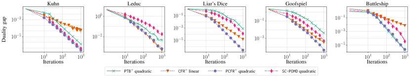
Figure 2: Convergence to Nash equilibrium as a function of number of iterations for PTB⁺ with quadratic averaging, CFR⁺ with linear averaging, PCFR⁺ with quadratic averaging, and SC-POMD with quadratic averaging. Every algorithm is using alternation.

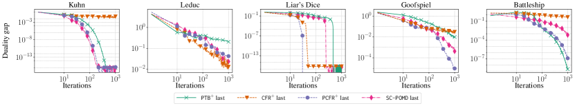
Figure 3: Convergence to Nash equilibrium for the last iterates of PTB⁺, CFR⁺, PCFR⁺, and SC-POMD. Every algorithm is using alternation.

We first determine the best way to instantiate our framework. We compare PTB⁺, Smooth PTB⁺ and AdaGradTB⁺ in the self-play framework with alternation (see Appendix A) and uniform, linear or quadratic weights for the iterates. PTB⁺ and Smooth PTB⁺ use the previous losses as predictions. We also study Treeplex Blackwell⁺ (TB⁺), corresponding to PTB⁺ without predictions ($\bm{m}_{t}=\bm{0}$), and AdamTB⁺, inspired by Adam Kingma and Ba (2015). For conciseness, we present our plots in Appendix I.3 (Figure 4) and state our conclusion here. We find that, for every game, PTB⁺ performs the best or is among the best algorithms. This underlines the advantage of treeplex stepsize invariance over algorithms that require tuning a stepsize (Smooth PTB⁺) and adaptive algorithms (AdaGradTB⁺), which may perform poorly due to the stepsize decreasing at a rate of $O(1/\sqrt{T})$. AdamTB⁺ does not even converge in some games.

We then compare the best of our algorithms (PTB⁺) with some of the best existing methods for solving EFGs: CFR⁺ (Tammelin et al., 2015), predictive CFR⁺ (PCFR⁺, Farina et al. (2021b), see Appendix B), and a version of optimistic online mirror descent with a single call to the orthogonal projection at every iteration (SC-POMD, Joulani et al. (2017)) achieving a $O(1/T)$ convergence rate; there are a variety of FOMs with a $O(1/T)$ rate, SC-POMD was observed to perform well in Chakrabarti et al. (2023). We determine the best empirical setup for each algorithm in Appendix I.4. In Figure 2, we compare the performance of the (weighted) average iterates. We find that PCFR⁺ outperforms both CFR⁺ and the theoretically-faster SC-POMD, as expected from past work. We had hoped to see at least comparable performance between PTB⁺ and PCFR⁺, since they are both based on Blackwell-approachability regret minimizers derived from applying POMD on the conic hull of their respective decision sets (simplexes at each infoset for PCFR⁺, treeplexes of each player for PTB⁺). However, in some games PCFR⁺ performs much better than PTB⁺. Given the similarity between PTB⁺ and PCFR⁺, our results suggest that the use of the CFR decomposition is part of the key to the performance of PCFR⁺. In particular, the CFR decomposition allows PCFR⁺ to have stepsize invariance at an infoset level, as opposed to stepsize invariance at the treeplex level in PTB⁺. Because of the structure of treeplexes, the numerical values of variables associated with infosets appearing late in the game, i.e., deeper in the treeplexes, may be much smaller than the numerical values of the variables appearing closer to the root. For this reason, allowing for different stepsizes at each infosets (like CFR⁺ and PCFR⁺ do) appears to be more efficient than using a single stepsize across all the infosets, even when the iterates do not depend on the value of this single stepsize (like in PTB⁺) and when this stepsize is fine-tuned (like in SC-POMD). Of course one could try to run SC-POMD with different stepsizes at each infoset and attempt to tune each of these stepsizes, but this is impossible in practical instances where the number of actions is large, e.g., $4.9\times 10^{4}$ actions in Liar’s Dice and $5.3\times 10^{6}$ actions in Goofspiel. CFR⁺ and PCFR⁺ bypass this issue with their infoset stepsize invariance, which enables both each infoset to have its own stepsize (via the CFR decomposition) and not needing to choose these stepsizes (via using RM⁺ and PRM⁺ as local regret minimizers, which are stepsize invariant).

We also investigate the performance of the last iterates in Figure 3. No algorithm appears to be the best across all game instances. CFR⁺ may not converge to a Nash equilibrium (e.g., on Kuhn), as has been observed before (Lee et al., 2021). PCFR⁺ exhibits linear convergence in some games (Kuhn, Liar’s Dice, Goofspiel) but not others (Leduc). The same is true for PTB⁺. Further investigations about last-iterate convergence are left as an important open question.

6 Conclusion

We propose the first Blackwell approachability-based regret minimizer over the treeplex (Algorithm 1) and we give several instantiations of our framework with different properties, including treeplex stepsize invariance (PTB⁺), adaptive stepsizes (AdaGradTB⁺) and achieving state-of-the-art $O(1/T)$ convergence guarantees on EFGs with a Blackwell approachability-based algorithm for the first time (Smooth PTB⁺). Since CFR⁺ and PCFR⁺ are stepsize invariant and have strong empirical performance, we were expecting PTB⁺ to have comparable performance. However, our experiments show that PTB⁺ often converges slower than CFR⁺ and PCFR⁺, so this stepsize invariance is not the only driver behind the practical performance of CFR⁺ and PCFR⁺. We view this negative result as an important contribution of our paper, since it rules out a previously plausible explanation for the practical performance of CFR⁺. Instead, we propose that one piece of the puzzle behind the CFR⁺ and PCFR⁺ performances is their infoset stepsize invariance, a consequence of combining the CFR framework with Blackwell approachability-based regret minimizers (RM⁺ and PRM⁺, themselves stepsize invariant over simplexes). Future works include better understanding the last-iterate performance of algorithms based on Blackwell approachability as well as the role of alternation.

Acknowledgments

Darshan Chakrabarti was supported by the National Science Foundation Graduate Research Fellowship Program under award number DGE-2036197. Julien Grand-Clément was supported by Hi! Paris and by a grant of the French National Research Agency (ANR), “Investissements d’Avenir” (LabEx Ecodec/ANR-11-LABX-0047). Christian Kroer was supported by the Office of Naval Research awards N00014-22-1-2530 and N00014-23-1-2374, and the National Science Foundation awards IIS-2147361 and IIS-2238960.

Appendix A Self-Play Framework

The (vanilla) self-play framework for two-player zero-sum EFGs is presented in Algorithm 5.

Algorithm 5 self-play framework

1:Input: ${\sf Regmin}_{\mathcal{X}}$ a regret minimizer over $\mathcal{X}$, ${\sf Regmin}_{\mathcal{Y}}$ a regret minimizer over $\mathcal{Y}$

2:for $t=1,\dots,T$ do

3:     $\bm{x}_{t}={\sf Regmin}_{\mathcal{X}}\left(\cdot\right)$

4:     $\bm{y}_{t}={\sf Regmin}_{\mathcal{Y}}\left(\cdot\right)$

5:     The first player observes the loss vector $\bm{Ay}_{t}\in\mathbb{R}^{n_{1}+1}$

6:     The second player observes the loss vector $-\bm{A}^{\top}\bm{x}_{t}\in\mathbb{R}^{n_{2}+1}$

The self-play framework can be combined with alternation, a simple variant that is known to lead to significant empirical speedups, for instance, when CFR⁺ and predictive CFR⁺ are used as regret minimizers [Tammelin et al., 2015, Farina et al., 2021b, Burch et al., 2019]. When using alternation, at iteration $t$ the second player is provided with the current strategy of the first player $\bm{x}_{t}$ before choosing its own strategy. We describe the self-play framework with alternation in Algorithm 6.

Algorithm 6 self-play framework with alternation

1:Input: ${\sf Regmin}_{\mathcal{X}}$ a regret minimizer over $\mathcal{X}$, ${\sf Regmin}_{\mathcal{Y}}$ a regret minimizer over $\mathcal{Y}$

2:for $t=1,\dots,T$ do

3:     $\bm{x}_{t}={\sf Regmin}_{\mathcal{X}}\left(\cdot\right)$

4:     The second player observes the loss vector $-\bm{A}^{\top}\bm{x}_{t}\in\mathbb{R}^{n_{2}+1}$

5:     $\bm{y}_{t}={\sf Regmin}_{\mathcal{Y}}\left(\cdot\right)$

6:     The first player observes the loss vector $\bm{Ay}_{t}\in\mathbb{R}^{n_{1}+1}$

Appendix B Counterfactual Regret Minimization (CFR), CFR⁺ and Predictive CFR⁺

Counterfactual Regret Minimization (CFR, Zinkevich et al. [2007]) is a framework for regret minimization over the treeplex. CFR runs a regret minimizer ${\sf Regmin}_{j}$ locally at each infoset $j\in\mathcal{J}$ of the treeplex. Note that here ${\sf Regmin}_{j}$ is a regret minimizer over the simplex $\Delta^{n_{j}}$ with $n_{j}=|\mathcal{A}_{j}|$, i.e., over the set of probability distributions over $\mathcal{A}_{j}$, the set of actions available at infoset $j\in\mathcal{J}$. Let $\bm{x}^{j}_{t}\in\Delta^{n_{j}}$ be the decision chosen by ${\sf Regmin}_{j}$ at iteration $t$ in CFR and let $\bm{\ell}_{t}\in\mathbb{R}^{n+1}$ be the loss across the entire treeplex. The local loss $\bm{\ell}_{t}^{j}\in\mathbb{R}^{n_{j}}$ that CFR passes to ${\sf Regmin}_{j}$ is

$$\ell_{t,a}^{j}:=\ell_{t,(j,a)}+\sum_{j^{\prime}\in\mathcal{C}_{ja}}V_{t}^{j^{\prime}},\forall\;a\in\mathcal{A}_{j},\forall\;j\in\mathcal{J}$$

where $V^{j}_{t}$ is the value function for infoset $j$ at iteration $t$, defined inductively:

$$V^{j}_{t}:=\sum_{a\in\mathcal{A}_{j}}x^{j}_{t,a}\ell_{t,(j,a)}+\sum_{j^{\prime}\in\mathcal{C}_{ja}}V_{t}^{j^{\prime}}.$$

The regret over the entire treeplex $\mathcal{T}$ can be related to the regrets accumulated at each infoset via the following laminar regret decomposition Farina et al. [2019a]:

$${\sf Reg}^{T}:=\max_{\hat{\bm{x}}\in\mathcal{T}}\sum_{t=1}^{T}\langle\bm{x}_{t}-\hat{\bm{x}},\bm{\ell}_{t}\rangle\leq\max_{\hat{\bm{x}}\in\mathcal{T}}\sum_{j\in\mathcal{J}}\hat{x}_{p_{j}}{\sf Reg}^{T}_{j}\left(\hat{\bm{x}}^{j}\right)$$

with ${\sf Reg}^{T}_{j}\left(\hat{\bm{x}}^{j}\right):=\sum_{t=1}^{T}\langle\bm{x}_{t}^{j}-\hat{\bm{x}}^{j},\bm{\ell}_{t}^{j}\rangle$ the regret incured by ${\sf Regmin}^{j}$ for the sequence of losses $\bm{\ell}_{1}^{j},...,\bm{\ell}_{T}^{j}$ against the comparator $\hat{\bm{x}}^{j}\in\Delta^{n_{j}}$. Combining CFR with regret minimizers at each information set ensures ${\sf Reg}^{T}=O\left(\sqrt{T}\right)$.

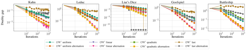
Figure 10: Convergence to Nash equilibrium as a function of number of iterations using uniform, linear, and quadratic averaging, as well as the last iterate, with and without alternation for CFR⁺.

CFR⁺ [Tammelin et al., 2015] corresponds to instantiating the self-play framework with alternation (Algorithm 6) and Regret Matching⁺ (RM⁺ as presented in (2.3)) as a regret minimizer at each information set. Additionally, CFR⁺ uses linear averaging, i.e., it returns $\bar{\bm{x}}_{T}$ such that $\bar{\bm{x}}_{T}=\frac{1}{\sum_{t=1}^{T}\omega_{t}}\sum_{t=1}^{T}\omega_{t}\bm{x}_{t}$ with $\omega_{t}=t$. We also consider uniform weights ($\omega_{t}=1$) and quadratic weights ($\omega=t^{2}$) in our simulations (Figure 10). CFR⁺ guarantees a $O(1/\sqrt{T})$ convergence rate to a Nash equilibrium.

Predictive CFR⁺(PCFR⁺, Farina et al. [2021b]) corresponds to instantiating the self-play framework with alternation (Algorithm 6) and Predictive Regret Matching⁺ (PRM⁺) as a regret minimizer at each information set. Given a simplex $\Delta^{d}$, PRM⁺ is a regret minimizer that returns a sequence of decisions $\bm{z}_{1},...,\bm{z}_{T}\in\Delta^{d}$ as follows:

$$\hat{\bm{R}}_{t} =\Pi_{\mathbb{R}_{+}^{d}}\left(\bm{R}_{t}-\eta\bm{g}(\bm{z}_{t-1},\bm{\ell}_{t-1})\right)$$ (PRM⁺)

$$\bm{z}_{t} =\hat{\bm{R}}_{t}/\|\hat{\bm{R}}_{t}\|_{1},$$

$$\bm{R}_{t+1} =\Pi_{\mathbb{R}_{+}^{d}}\left(\bm{R}_{t}-\eta\bm{g}(\bm{z}_{t},\bm{\ell}_{t})\right)$$

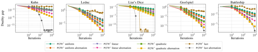
Figure 11: Convergence to Nash equilibrium as a function of number of iterations using uniform, linear, and quadratic averaging, as well as the last iterate, with and without alternation for PCFR⁺.

where the function $g$ is defined in (2.4). Similar to CFR⁺, for PCFR⁺ we investigate different weighting schemes in our numerical experiments (Figure 11). It is not known if the self-play framework with alternation, combined with PCFR⁺, has convergence guarantees, but PCFR⁺ has been observed to achieve state-of-the-art practical performance in many EFG instances Farina et al. [2021b].

Appendix C Proof of Proposition 4.1

Proof.

The proof of Proposition 4.1 is based on the following lemma.

Lemma C.1.

Let $\mathcal{C}\subset\mathbb{R}^{n}$ be a convex cone and let $\bm{u}\in\mathbb{R}^{n},\eta>0$. Then

$$\Pi_{\mathcal{C}}(\eta\bm{u})=\eta\Pi_{\mathcal{C}}(\bm{u}).$$

Proof of Lemma C.1.

We have, by definition,

$$\Pi_{\mathcal{C}}(\eta\bm{u})=\arg\min_{\bm{R}\in\mathcal{C}}\|\bm{R}-\eta\bm{u}\|_{2}.$$

Now we also have

$$\min_{\bm{R}\in\mathcal{C}}\|\bm{R}-\eta\bm{u}\|_{2}=\eta\cdot\min_{\bm{R}\in\mathcal{C}}\|\frac{1}{\eta}\bm{R}-\bm{u}\|_{2}=\eta\cdot\min_{\bm{R}\in\mathcal{C}}\|\bm{R}-\bm{u}\|_{2}$$

where the last equality follows from $\mathcal{C}$ being a cone. This shows that $\arg\min_{\bm{R}\in\mathcal{C}}\|\bm{R}-\eta\bm{u}\|_{2}$ is attained at $\eta\Pi_{\mathcal{C}}(\bm{u})$, i.e., that $\Pi_{\mathcal{C}}(\eta\bm{u})=\eta\Pi_{\mathcal{C}}(\bm{u})$. ∎

We are now ready to prove Proposition 4.1. For the sake of conciseness we prove this with $\bm{m}_{1}=...=\bm{m}_{T}=\bm{0}$; the proof for PTB⁺ with predictions is identical. In this case, $\bm{R}_{t}=\hat{\bm{R}}_{t},\forall\;t\geq 1$. Consider the sequence of strategies $\tilde{\bm{x}}_{1},...,\tilde{\bm{x}}_{T}$ and $\tilde{\bm{R}}_{1},...,\tilde{\bm{R}}_{T}$ generated by PTB⁺ with a step size of $1$. We also consider the sequence of strategies $\bm{x}_{1},...,\bm{x}_{T}$ and $\bm{R}_{1},...,\bm{R}_{T}$ generated with a step size $\eta>0$. We claim that

$$\tilde{\bm{x}}_{t}=\bm{x}_{t},\bm{R}_{t}=\eta\tilde{\bm{R}}_{t},\;\forall\;t\in\{1,...,T\}.$$

We prove this by induction. Both sequences of iterates are initialized with $\bm{R}_{1}=\tilde{\bm{R}}_{1}=\bm{0}$ so that $\tilde{\bm{x}}_{1}=\bm{x}_{1}$. Therefore, both sequences face the same loss $\bm{\ell}_{1}$ at $t=1$, and we have

$$\bm{R}_{2}=\Pi_{\mathcal{C}}(-\eta\bm{f}(\bm{x}_{1},\bm{\ell}_{1}))=\eta\pi_{\mathcal{C}}(-\bm{f}(\bm{x}_{1},\bm{\ell}_{1})))=\eta\tilde{\bm{R}}_{2}.$$

Let us now consider an iteration $t\geq 1$ and suppose that $\tilde{\bm{x}}_{t}=\bm{x}_{t},\bm{R}_{t}=\eta\tilde{\bm{R}}_{t}$. Since $\tilde{\bm{x}}_{t}=\bm{x}_{t}$ then both algorithms will face the next loss vector $\bm{\ell}_{t}$. Then

$$\bm{R}_{t+1} =\pi_{\mathcal{C}}(\bm{R}_{t}-\eta\bm{f}(\bm{x}_{t},\bm{\ell}_{t}))$$

$$=\pi_{\mathcal{C}}(\eta\tilde{\bm{R}}_{t}-\eta\bm{f}(\bm{x}_{t},\bm{\ell}_{t}))$$

$$=\eta\pi_{\mathcal{C}}(\tilde{\bm{R}}_{t}-\bm{f}(\bm{x}_{t},\bm{\ell}_{t}))$$

$$=\eta\tilde{\bm{R}}_{t+1}$$

which in turns implies that $\bm{x}_{t+1}=\tilde{\bm{x}}_{t+1}$. We conclude that $\bm{x}_{t}=\tilde{\bm{x}}_{t},\forall\;t=1,...,T$. ∎

Appendix D Comparison Between RM⁺ and PTB⁺

Assume that the original decision set of each player is a simplex $\Delta^{d}$ and that there are no predictions: $\bm{m}_{t}=\bm{0},\forall\;t\geq 1$.

PTB⁺ over the simplex.

For PTB⁺, the empty sequence variable $x_{\varnothing}$ is introduced and appended to the decision $\Delta^{d}$. The resulting treepplex can be written $\mathcal{T}=\{1\}\times\Delta^{d}$, the set $\mathcal{C}$ becomes $\mathcal{C}:={\sf cone}(\mathcal{T})={\sf cone}(\{1\}\times\Delta^{d})$ and $\bm{a}=(1,\bm{0})\in\mathbb{R}^{d+1}_{+}$ with $1$ on the first component related to $x_{\varnothing}$ and $0$ everywhere else. In this case, PTB⁺ without prediction is exactly the Conic Blackwell Algorithm⁺ (CBA⁺, Grand-Clément and Kroer [2023]). Crucially, to run PTB⁺ we need to compute the orthogonal projection onto ${\sf cone}(\mathcal{T})={\sf cone}(\{1\}\times\Delta)$ at every iteration, which can not be computed in closed-form, but it can be computed in $O(n\log(n))$ arithmetic operations (see Appendix G.1 in Grand-Clément and Kroer [2023]).

Regret Matching⁺.

RM⁺ operates directly over the simplex $\Delta^{d}$ without the introduction of the empty sequence $x_{\varnothing}$, in contrast to PTB⁺ which operates over $\{1\}\times\Delta^{d}$. Importantly, in RM⁺, at every iteration the orthogonal projection onto $\mathbb{R}^{d}_{+}$ can be computed in closed form by simply thresholding to zero the negative components (and leaving unchanged the positive components): $\Pi_{\mathbb{R}_{+}^{d}}\left(\bm{z}\right)=\left(\max\{z_{i},0\}\right)_{i\in[d]}$ for any $\bm{z}\in\mathbb{R}^{d}$.

Empirical comparisons.

The numerical experiments in Grand-Clément and Kroer [2023] show that CBA⁺ may be slightly faster than RM⁺ for some matrix games in terms of speed of convergence as a function of the number of iterations, but it can be slower in running times because of the orthogonal projections onto ${\sf cone}(\{1\}\times\Delta)$ at each iteration (Figures 2,3,4 in Grand-Clément and Kroer [2023]). When $\mathcal{T}$ is a treeplex that is not the simplex, introducing $x_{\varnothing}$ also changes the resulting algorithm but not the complexity of the orthogonal projection onto ${\sf cone}(\mathcal{T})$, since there is no closed-form anymore, even without $x_{\varnothing}$. As a convention, in this paper, we will always use $x_{\varnothing}$ in our description of treeplexes and of our algorithms since it is convenient from a writing and implementation standpoint.

Overall, we notice that in the case of the simplex introducing the empty sequence variable $x_{\varnothing}$ radically alters the complexity per iterations and the resulting algorithm, a fact that has not been noticed in previous work.

Appendix E Proof of Proposition 4.5

Proof of Proposition 4.5.

1. Let $\hat{\bm{R}}_{2}=\bm{R}_{2}/\|\bm{R}_{2}\|_{2}$ be the unit vector pointing in the same direction as $\bm{R}_{2}$ and let $\bm{h}:=\left(\langle\bm{R}_{1},\hat{\bm{R}_{2}}\rangle\right)\hat{\bm{R}_{2}}$ the orthogonal projection of $\bm{R}_{1}$ onto $\{\alpha\hat{\bm{R}}_{2}\;|\;\alpha\in\mathbb{R}\}$. We thus have $\|\bm{R}_{1}-\bm{R}_{2}\|_{2}\geq\|\bm{R}_{1}-\bm{h}\|_{2}$.

2. Let $\bm{p}=\frac{\langle\bm{R}_{1},\bm{a}\rangle}{\langle\bm{R}_{2},\bm{a}\rangle}\hat{\bm{R}}_{2}$. Since $\bm{p}$ and $\bm{R}_{2}$ are colinear, we have

   $$\left\|\frac{\bm{R}_{1}}{\langle\bm{R}_{1},\bm{a}\rangle}-\frac{\bm{R}_{2}}{\langle\bm{R}_{2},\bm{a}\rangle}\right\|_{2}=\left\|\frac{\bm{R}_{1}}{\langle\bm{R}_{1},\bm{a}\rangle}-\frac{\bm{p}}{\langle\bm{p},\bm{a}\rangle}\right\|_{2}.$$

   Additionally, by construction, $\langle\bm{p},\bm{a}\rangle=\langle\bm{R}_{1},\bm{a}\rangle$, so that we obtain

   $$\left\|\frac{\bm{R}_{1}}{\langle\bm{R}_{1},\bm{a}\rangle}-\frac{\bm{R}_{2}}{\langle\bm{R}_{2},\bm{a}\rangle}\right\|_{2}=\left\|\frac{\bm{R}_{1}}{\langle\bm{R}_{1},\bm{a}\rangle}-\frac{\bm{p}}{\langle\bm{R}_{1},\bm{a}\rangle}\right\|_{2}=\frac{1}{\langle\bm{R}_{1},\bm{a}\rangle}\|\bm{R}_{1}-\bm{p}\|_{2}.$$

   Note that $\langle\bm{R}_{1},\bm{a}\rangle\geq 0$ since $\bm{R}_{1}\in{\sf cone}(\mathcal{T})$ and $\mathcal{T}\subset\{\bm{x}\in\mathbb{R}^{n+1}\;|\;\langle\bm{x},\bm{a}\rangle=1\}$. Assume that we can compute $D>0$ such that $\frac{\|\bm{R}_{1}-\bm{p}\|_{2}}{\|\bm{R}_{1}-\bm{h}\|_{2}}\leq D$. Then we have

   $$\left\|\frac{\bm{R}_{1}}{\langle\bm{R}_{1},\bm{a}\rangle}-\frac{\bm{R}_{2}}{\langle\bm{R}_{2},\bm{a}\rangle}\right\|_{2}\leq\frac{D}{\langle\bm{R}_{1},\bm{a}\rangle}\|\bm{R}_{1}-\bm{h}\|_{2}\leq\frac{D}{\langle\bm{R}_{1},\bm{a}\rangle}\|\bm{R}_{1}-\bm{R_{2}}\|_{2}.$$

3. The rest of this proof focuses on showing that $\frac{\|\bm{R}_{1}-\bm{p}\|_{2}}{\|\bm{R}_{1}-\bm{h}\|_{2}}\leq\Omega$ with $\Omega=\max\{\|\bm{x}\|_{2}|\;\bm{x}\in\mathcal{T}\}$. Note that $\langle\bm{R}_{1}-\bm{p},\bm{a}\rangle=0$. Therefore, $\frac{1}{\|\bm{R}_{1}-\bm{p}\|_{2}}\left(\bm{R}_{1}-\bm{p}\right)$ and $\frac{1}{\|\bm{a}\|_{2}}\bm{a}$ can be completed to form an orthonormal basis of $\mathbb{R}^{n}$. In this basis, we have

   $$\|\hat{\bm{R}_{2}}\|_{2}^{2}\geq\frac{\left(\langle\bm{R}_{1}-\bm{p},\hat{\bm{R}_{2}}\rangle\right)^{2}}{\|\bm{R}_{1}-\bm{p}\|_{2}^{2}}+\frac{\left(\langle\bm{a},\hat{\bm{R}_{2}}\rangle\right)^{2}}{\|\bm{a}\|_{2}^{2}}.$$

   Note that by construction we have $\|\hat{\bm{R}_{2}}\|_{2}^{2}=1$. Additionally, $\bm{R}_{2}\in{\sf cone}(\mathcal{T})$ so that there exists $\alpha>0$ and $\bm{y}\in\mathcal{T}$ such that $\bm{R}_{2}=\alpha\bm{x}$. By construction of $\hat{\bm{R}}_{2}$, we have $\hat{\bm{R}}_{2}=\frac{\alpha\bm{x}}{\|\alpha\bm{x}\|_{2}}=\frac{\bm{x}}{\|\bm{x}\|_{2}}$ and $\langle\bm{x},\bm{a}\rangle=1$. This shows that

   $$\frac{\left(\langle\bm{a},\hat{\bm{R}_{2}}\rangle\right)^{2}}{\|\bm{a}\|_{2}^{2}}=\frac{\left(\langle\bm{a},\bm{x}\rangle\right)^{2}}{\|\bm{a}\|_{2}^{2}\|\bm{x}\|_{2}^{2}}=\frac{1}{\|\bm{a}\|_{2}^{2}\|\bm{x}\|_{2}^{2}}\geq\frac{1}{\Omega\|\bm{a}\|_{2}^{2}}$$

   with $\Omega=\max\{\|\bm{x}\|_{2}|\;\bm{x}\in\mathcal{T}\}$. Recall that we have chosen $\bm{a}=(1,\bm{0})$ so that $\|\bm{a}\|_{2}=1$. Overall, we have obtained

   $$1-\frac{1}{\Omega^{2}}\geq\frac{\left(\langle\bm{R}_{1}-\bm{p},\hat{\bm{R}_{2}}\rangle\right)^{2}}{\|\bm{R}_{1}-\bm{p}\|_{2}^{2}}.$$

   From the definition of the vectors $\bm{p},\bm{h}$ and $\hat{\bm{R}_{2}}$, we have

   $$\frac{\left(\langle\bm{R}_{1}-\bm{p},\hat{\bm{R}_{2}}\rangle\right)^{2}}{\|\bm{R}_{1}-\bm{p}\|_{2}^{2}}=\frac{\|\bm{p}-\bm{h}\|_{2}^{2}}{\|\bm{R_{1}}-\bm{p}\|_{2}^{2}}.$$

   Hence, we have

   $$\|\bm{p}-\bm{h}\|_{2}^{2}\leq\left(1-\frac{1}{\Omega^{2}}\right)\|\bm{R}_{1}-\bm{p}\|_{2}^{2}.$$

   This shows that $\|\bm{R}_{1}-\bm{h}\|_{2}^{2}\geq\frac{1}{\Omega^{2}}\|\bm{x}-\bm{p}\|_{2}^{2}$.

4. We conclude that

   $$\left\|\frac{\bm{R}_{1}}{\langle\bm{R}_{1},\bm{a}\rangle}-\frac{\bm{R}_{2}}{\langle\bm{R}_{2},\bm{a}\rangle}\right\|_{2}\leq\frac{\Omega}{\max\{\langle\bm{R}_{1},\bm{a}\rangle,\langle\bm{R}_{2},\bm{a}\rangle\}}\|\bm{R}_{1}-\bm{R}_{2}\|_{2}.$$

∎

Appendix F Proof of Proposition 4.4

In this section we show how to efficiently compute the orthogonal projection onto the cone $\mathcal{C}:={\sf cone}(\mathcal{T})$. We start by reviewing the existing methods for computing the orthogonal projection onto the treeplex $\mathcal{T}$. This is an important cornerstone of our analysis, since the treeplex $\mathcal{T}$ and the cone $\mathcal{C}$ share an analogous structure:

$$\mathcal{T} =\{\bm{x}\in\mathbb{R}^{n+1}_{+}\;|\;x_{\varnothing}=1,\sum_{a\in\mathcal{A}_{j}}x_{ja}=x_{p_{j}},\forall\;j\in\mathcal{J}\}$$

$$\mathcal{C} =\{\bm{x}\in\mathbb{R}^{n+1}_{+}\;|\;\sum_{a\in\mathcal{A}_{j}}x_{ja}=x_{p_{j}},\forall\;j\in\mathcal{J}\}.$$

Gilpin et al. [2012] were the first to show an algorithm for computing Euclidean projection onto the treeplex. They do this by defining a value function for the projection of a given point $\bm{y}$ onto the closed and convex scaled set $t\mathcal{Z}$, letting it be half the squared distance between $\bm{y}$ and $t\mathcal{Z}$, for $t\in\mathbb{R}_{>0}$:

$$v_{\mathcal{Z}}(t,\bm{y}):=\frac{1}{2}\min_{\bm{z}\in t\mathcal{Z}}\|\bm{z}-\bm{y}\|^{2}_{2}.$$

Gilpin et al. [2012] show how to recursively compute $\lambda_{\mathcal{Z}}(t,\bm{y})$, the derivative of this function with respect to $t$, for a given treeplex, since treeplexes can be constructed recursively using two operations: branching and Cartesian product. In the first case, given $k$ treeplexes $\mathcal{Z}_{1},\dots,\mathcal{Z}_{k}$, then $\mathcal{Z}=\{\bm{x},\bm{x}[1]\bm{z}_{1},\dots,\bm{x}[k]\bm{z}_{k}:x\in\Delta_{k},\bm{z}_{i}\in\mathcal{Z}_{i}\forall i\in[k]\}$ is also a treeplex. In the second case, given $k$ treeplexes $\mathcal{Z}_{1},\dots,\mathcal{Z}_{k}$, then $\mathcal{Z}=\mathcal{Z}_{1}\times\cdots\times\mathcal{Z}_{k}$ is also a treeplex. In fact, letting the empty set be a treeplex as a base case, all treeplexes can be constructed in this way.

However, Gilpin et al. [2012] did not state the total complexity of computing the projection, instead only stating the complexity of computing $\lambda_{\mathcal{Z}}(t,\bm{y})$ given the corresponding $\lambda_{\mathcal{Z}_{i}}(t,\bm{y}_{i})$ functions for the treeplexes $\mathcal{Z}_{i}$ that are used to construct $\mathcal{Z}$ using $i\in[k]$. They state that this complexity is $O(n\log n)$, where $n$ is the number of sequences in $\mathcal{Z}$. Their analysis involves showing that the function $t\mapsto\lambda_{\mathcal{Z}}(t,\bm{y})$ is piecewise linear.

Farina et al. [2022] also consider this problem, generalizing the problem to weighted projection on the scaled treeplex, by adding an additional positive parameter $\bm{w}\in\mathbb{R}^{n}_{>0}$:

$$v_{\mathcal{Z}}(t,\bm{y},\bm{w}):=\frac{1}{2}\min_{\bm{z}\in t\mathcal{Z}}\sum_{i=1}^{n}\left(\bm{z}[i]-\frac{\bm{y}[i]}{\bm{w}[i]}\right)^{2}.$$

They do a similar analysis to Gilpin et al. [2012], by showing how to compute the derivative $\lambda_{\mathcal{Z}}(t,\bm{y},\bm{w})$ of $v_{\mathcal{Z}}(t,\bm{y},\bm{w})$ with respect to $t$ recursively. They show that $t\mapsto\lambda_{\mathcal{Z}}(t,\bm{y},\bm{w})$ are strictly-monotonically-increasing piecewise-linear (SMPL) functions. We will follow the analysis in Farina et al. [2022], letting $\bm{w}=\mathbf{1}$.

We first define a standard representation of a SMPL function.

Definition F.1 ([Farina et al., 2022]).

Given a SMPL function $f$, a standard representation is an expression of the form

$$f(x)=\zeta+\alpha_{0}x+\sum_{s=1}^{S}\alpha_{s}\max\{0,x-\beta_{s}\}$$

valid for all $x\in\operatorname{dom}(f)$, $S\in\mathbb{N}\cup\{0\}$, and $\beta_{1}<\cdots<\beta_{S}$. The size of the standard representation is defined to be $S$.

Next, we prove the following lemma, showing the computational complexity of computing the derivative of the value function for a given treeplex.

Lemma F.2.

For a given treeplex $\mathcal{Z}$ with depth $d$, $n$ sequences, $l$ leaf sequences, and $m$ infosets, and $\bm{y}\in\mathbb{R}^{n},\bm{w}\in\mathbb{R}^{n}_{>0}$, a standard representation of $\lambda_{\mathcal{Z}}(t,\bm{y},\bm{w})$ can be computed in $O\big{(}dn\log(l+m)\big{)}$ time.

Proof.

We will proceed by structural induction over treeplexes, following the analysis done by Farina et al. [2022]. The base case is trivially true, because the empty set has no sequences or depth.

For the inductive case, we will assume that it requires $O\big{(}(d-1)n\log(l+m)\big{)}$ time to compute the respective Euclidean projections onto the subtreeplexes that we use to inductively construct our current treeplex, where $d-1$ is the depth of a given subtreeplex, $n$ is the number of sequences in the subtreeplex, and $m$ is the total number of sequences among both players and chance corresponding to the game from which the treeplex originates.

We will use two results shown in Lemma 14 of Farina et al. [2022]:

Lemma F.3 (Recursive complexity of Euclidean projection for branching operation [Farina et al., 2022]).

Consider a treeplex $\mathcal{Z}$ that can be written as the result of a branching operation on $k$ treeplexes $\mathcal{Z}_{1},\dots,\mathcal{Z}_{k}$:

$$\mathcal{Z}=\{\bm{x},\bm{x}[1]\bm{z}_{1},\dots,\bm{x}[k]\bm{z}_{k}:x\in\Delta_{k},\bm{z}_{i}\in\mathcal{Z}_{i}\forall i\in[k]\}.$$

Let $\mathcal{Z}$ have $n$ sequences and let $\bm{y},\bm{w}\in\mathbb{R}^{n}$, and let $\bm{y}[i]$ and $\bm{w}[i]$ denote the corresponding respective components of $\bm{y}$ and $\bm{w}$ for the treeplex $\mathcal{Z}_{i}$.

Then, given standard representations of $\lambda_{\mathcal{Z}_{i}}(t,\bm{y}_{i},\bm{w}_{i})$ of size $n_{i}$ for all $i\in[k]$, where $n_{i}$ is the number of sequences that $\mathcal{Z}_{i}$ has, a standard representation of $\lambda_{\mathcal{Z}}(t,\bm{y},\bm{w})$ of size $n$ can be computed in $O(n\log k)$ time.

Furthermore, given a value of $t$, the argument $\bm{x}$ which leads to the realization of the optimal value of the value function, can be computed in time $O(n)$.

Lemma F.4 (Recursive complexity of Euclidean projection for Cartesian product [Farina et al., 2022]).

Consider a treeplex $\mathcal{Z}$ that can be written as a Cartesian product of $k$ treeplexes $\mathcal{Z}_{1},\dots,\mathcal{Z}_{k}$:

$$\mathcal{Z}=\mathcal{Z}_{1}\times\cdots\times\mathcal{Z}_{k}.$$

Let $\mathcal{Z}$ have $n$ sequences and let $\bm{y},\bm{w}\in\mathbb{R}^{n}$, and let $\bm{y}[i]$ and $\bm{w}[i]$ denote the corresponding respective components of $\bm{y}$ and $\bm{w}$ for the treeplex $\mathcal{Z}_{i}$.

Then, given standard representations of $\lambda_{\mathcal{Z}_{i}}(t,\bm{y}_{i},\bm{w}_{i})$ of size $n_{i}$ for all $i\in[k]$, where $n_{i}$ is the number of sequences that $\mathcal{Z}_{i}$ has, a standard representation of $\lambda_{\mathcal{Z}}(t,\bm{y},\bm{w})$ of size $n$ can be computed in $O(n\log k)$ time.

First, we consider the case that the last operation used to construct our treeplex was the branching operation. Let the root of of the treeplex be called $j$. Define $\mathcal{Z}_{i}$ as the treeplex that is underneath action $a_{i}\in\mathcal{A}_{j}$. Let $n_{i}$ denote the number of sequences in $\mathcal{Z}_{i}$, $m_{i}$ denote the number of infosets in $\mathcal{Z}_{i}$, $l_{i}$ denote the number of leaf sequences in $\mathcal{Z}_{i}$, and $d-1$ be the maximum depth of any of these subtreeplexes.

Given a standard representation of $\lambda_{\mathcal{Z}_{i}}(t,\bm{y}_{i},\bm{w}_{i})$ of size $n_{i}$ for all $i\in[|\mathcal{A}_{j}|]$, by Lemma F.3, it takes $O(n\log|\mathcal{A}_{j}|)$ time to compute a standard representation of $\lambda_{\mathcal{Z}}(t,\bm{y},\bm{w})$ of size $n$. By induction, it takes $O\big{(}(d-1)n_{i}\log m_{i}\big{)}$ to compute $\lambda_{\mathcal{Z}_{i}}(t,\bm{y}_{i},\bm{w}_{i})$ for treeplex $\mathcal{Z}_{i}$. Thus the total computation required to compute $\lambda_{\mathcal{Z}}(t,\bm{y},\bm{w})$ is

$$O(n\log|\mathcal{A}_{j}|)+\sum_{i\in[|\mathcal{A}_{j}|]}O\big{(}(d-1)n_{i}\log(l_{i}+m_{i})\big{)} =O(n\log|\mathcal{A}_{j}|)+\sum_{i\in[|\mathcal{A}_{j}|]}O\big{(}(d-1)n_{i}\log(l+m)\big{)}$$

$$=O(n\log|\mathcal{A}_{j}|)+O\big{(}(d-1)\sum_{i\in[|\mathcal{A}_{j}|]}n_{i}\log(l+m)\big{)}$$

$$=O(n\log|\mathcal{A}_{j}|)+O\big{(}(d-1)n\log(l+m)\big{)}$$

$$=O\big{(}n\log(l+m)\big{)}+O\big{(}(d-1)n\log(l+m)\big{)}$$

$$=O\big{(}dn\log(l+m)\big{)}$$

since we have necessarily that $l_{i}\leq l$ and $m_{i}\leq m$ for all $i\in[|\mathcal{A}_{j}|]$, $\sum_{i\in[|\mathcal{A}_{j}|]}n_{i}\leq n$, and $|\mathcal{A}_{j}|\leq l+m$.

Second, we consider the case the last operation to construct our treeplex was a Cartesian product. Let $\mathcal{Z}=\mathcal{Z}_{1}\times\cdots\times\mathcal{Z}_{k}$, and again define $n_{i}$ as the number of sequences in $\mathcal{Z}_{i}$, $m_{i}$ as the number of infosets in $\mathcal{Z}_{i}$, $l_{i}$ as the number of leaf sequences in $\mathcal{Z}_{i}$, and $d-1$ as the maximum depth of any of these subtreeplexes.

Given a standard representation of $\lambda_{\mathcal{Z}_{i}}(t,\bm{y}_{i},\bm{w}_{i})$ of size $n_{i}$ for all $i\in[k]$, by Lemma F.4 it takes $O(n\log k)$ to compute a standard representation of $\lambda_{\mathcal{Z}}(t,\bm{y},\bm{w})$ of size $n$. By induction, it takes $O\big{(}(d-1)n_{i}\log(l_{i}+m_{i})\big{)}$ to compute $\lambda_{\mathcal{Z}_{i}}(t,\bm{y}_{i},\bm{w}_{i})$ for treeplex $\mathcal{Z}_{i}$. Thus the total computation required to compute $\lambda_{\mathcal{Z}}(t,\bm{y},\bm{w})$ is

$$O(n\log k)+\sum_{i\in[k]}O\big{(}(d-1)n_{i}\log(l_{i}+m_{i})\big{)} =O(n\log k)+\sum_{i\in[k]}O\big{(}(d-1)n_{i}\log(l+m)\big{)}$$

$$=O(n\log k)+O\big{(}(d-1)\sum_{i\in[k]}n_{i}\log(l+m)\big{)}$$

$$=O(n\log k)+O\big{(}(d-1)n\log(l+m)\big{)}$$

$$=O(n\log m)+O\big{(}(d-1)n\log(l+m)\big{)}$$

$$=O(dn\log(l+m))$$

since we have necessarily that $l_{i}\leq l$ and $m_{i}\leq m$ for all $i\in[k]$, and $k\leq m$. ∎

Finally, we are ready to prove the main statement.

Proof of Proposition 4.4.

By Lemma F.2, we know that we can recursively compute a standard representation of $\lambda_{\mathcal{Z}}(t,\bm{y},\bm{w})$ in $O\big{(}dn\log(l+m)\big{)}$ time. Assuming we use this construction, invoking Lemma F.3, given an optimal value of $t$, we can compute the partial argument corresponding to the values of the sequences that originate at the root infosets, which allow the optimal value to be realized for the value function. Then, we can use optimal arguments for these sequences recursively at the subtreeplexes to continue computing the optimal argument at sequences lower on the treeplex. We can do this because in the process of computing the derivative of the value function of the entire treeplex, we have also computed the derivative of the value function for each of the subtreeplexes. Thus, once we have computed an optimval value of $t$ for the value function at the top level, we can do a top-down pass to compute the optimal values for all sequences that occur at any level in the treeplex. This is detailed in the analysis done in the proof of Lemma 14 in Farina et al. [2022].

In order to pick the optimal value of $t$ for the value function, since $\lambda_{\mathcal{Z}}(\cdot,\bm{y},\bm{w})$ is strictly increasing, we only have to consider two cases: $\lambda_{\mathcal{Z}}(0,\bm{y},\bm{w})<0$ and $\lambda_{\mathcal{Z}}(0,\bm{y},\bm{w})\geq 0$. In the first case, the value function $\lambda_{\mathcal{Z}}(\cdot,\bm{y},\bm{w})$ will be minimized when $\lambda_{\mathcal{Z}}(\cdot,\bm{y},\bm{w})$ is equal to $0$, and this can be directly computed using the standard representation (it will be necessarily $0$ somewhere because it is strictly monotone). In the second case, since $\lambda_{\mathcal{Z}}(\cdot,\bm{y},\bm{w})$ is strictly monotone and $\lambda_{\mathcal{Z}}(0,\bm{y},\bm{w})\geq 0$, we must have that $\lambda_{\mathcal{Z}}(\cdot,\bm{y},\bm{w})\geq 0$, which means that $v_{\mathcal{Z}}(\cdot,\bm{y},\bm{w})$ is minimized at $t^{*}=0$. ∎

Appendix G Practical Implementation of Smooth PTB⁺

We have the following lemma, which shows that the stable region $\mathcal{C}_{\geq}$ admits a relatively simple formulation.

Lemma G.1.

The stable region

$$\mathcal{C}_{\geq}:={\sf cone}(\mathcal{T})\cap\{\bm{R}\in\mathbb{R}^{n+1}\;|\;\langle\bm{R},\bm{a}\rangle\geq R_{0}\}$$

can be reformulated as follows:

$$\mathcal{C}_{\geq} =\{\alpha\bm{x}\;|\;\alpha\geq R_{0},\bm{x}\in\mathcal{T}\}$$

$$=\{\bm{x}\in\mathbb{R}^{n+1}_{+}\;|x_{\varnothing}\geq R_{0},\sum_{a\in\mathcal{A}_{j}}x_{ja}=x_{p_{j}},\forall\;j\in\mathcal{J}\}.$$

Proof.

By definition, we have

$$\mathcal{C}_{\geq}=\{\bm{R}\in{\sf cone}(\mathcal{T})\;|\;\langle\bm{R},\bm{a}\rangle\geq R_{0}\}.$$

Note that for $\bm{R}\in{\sf cone}(\mathcal{T}),\bm{R}=\alpha\bm{x}$ with $\alpha\geq 0$ and $\langle\bm{x},\bm{a}\rangle=1$. Therefore, for $\bm{R}\in\mathcal{C}$ we have $\langle\bm{R},\bm{a}\rangle\geq R_{0}\iff\alpha\geq R_{0}$. This shows that we can write

$$\mathcal{C}_{\geq}=\{\alpha\bm{x}\;|\;\alpha\geq R_{0},\bm{x}\in\mathcal{T}\}.$$

Now let $\bm{x}\in\mathcal{C}_{\geq}$, i.e., let $\bm{x}=\alpha\hat{\bm{x}}$ with $\alpha\geq R_{0}$ and $\bm{x}\in\mathcal{T}$. Since $\hat{\bm{x}}\in\mathcal{T}$, we have $x_{\varnothing}=1$, so that $\hat{x}_{\varnothing}=\alpha\geq R_{0}$. Additionally, we have $\hat{\bm{x}}\geq 0,\sum_{a\in\mathcal{A}_{j}}\hat{x}_{ja}=\hat{x}_{p_{j}},\forall\;j\in\mathcal{J}$. Multiplying by $\alpha\geq R_{0}$, we obtain that $\bm{x}\geq 0$ and $\sum_{a\in\mathcal{A}_{j}}x_{ja}=x_{p_{j}},\forall\;j\in\mathcal{J}$. Overall we have shown

$$\mathcal{C}_{\geq}\subseteq\{\bm{x}\in\mathbb{R}^{n+1}\;|x_{\varnothing}\geq R_{0},\sum_{a\in\mathcal{A}_{j}}x_{ja}=x_{p_{j}},\forall\;j\in\mathcal{J},\bm{x}\geq\bm{0}\}.$$

We now consider $\bm{x}\in\{\bm{x}\in\mathbb{R}^{n+1}\;|x_{\varnothing}\geq R_{0},\sum_{a\in\mathcal{A}_{j}}x_{ja}=x_{p_{j}},\forall\;j\in\mathcal{J},\bm{x}\geq\bm{0}\}$ with $\bm{x}\neq\bm{0}$. Then $\bm{x}=\alpha\frac{\bm{x}}{\alpha}$ with $\alpha=x_{\varnothing}$, so that $\alpha\geq R_{0}$ and

$$\sum_{a\in\mathcal{A}_{j}}x_{ja}=x_{p_{j}},\forall\;j\in\mathcal{J}\iff\sum_{a\in\mathcal{A}_{j}}\frac{x_{ja}}{\alpha}=\frac{x_{p_{j}}}{\alpha},\forall\;j\in\mathcal{J}.$$

Therefore

$$\{\bm{x}\in\mathbb{R}^{n+1}\;|x_{\varnothing}\geq R_{0},\sum_{a\in\mathcal{A}_{j}}x_{ja}=x_{p_{j}},\forall\;j\in\mathcal{J},\bm{x}\geq\bm{0}\}\subseteq\mathcal{C}_{\geq}.$$

This shows that we have

$$\mathcal{C}_{\geq}=\{\bm{x}\in\mathbb{R}^{n+1}\;|x_{\varnothing}\geq R_{0},\sum_{a\in\mathcal{A}_{j}}x_{ja}=x_{p_{j}},\forall\;j\in\mathcal{J},\bm{x}\geq\bm{0}\}.$$

∎

Proposition G.2.

For a treeplex $\mathcal{T}$ with depth $d$, number of sequences $n$, number of leaf sequences $l$, and number of infosets $m$, the complexity of computing the orthogonal projection of a point $y\in\mathbb{R}^{n+1}$ onto $\mathcal{C}_{\geq}=\{\alpha\bm{x}\;|\;\alpha\geq R_{0},\bm{x}\in\mathcal{T}\}$ is $O\big{(}dn\log(l+m)\big{)}$.

Proof.

The proof is the same as that for Proposition 4.4, since the derivative of the value function can be computed in $O\big{(}dn\log(l+m)\big{)}$ time. However, this time, we have an additional constraint that $t\geq R_{0}$. Thus instead of checking the sign of $\lambda_{\mathcal{Z}}(\cdot,\bm{y},\bm{w})$ at $t=0$, we check the sign at $R_{0}$.

If $\lambda_{\mathcal{Z}}(R_{0},\bm{y},\bm{w})<0$, then because $\lambda_{\mathcal{Z}}(\cdot,\bm{y},\bm{w})$ is a strictly monotone function, the function will be $0$ for some value of $t$, and this is exactly $t^{*}$, which minimizes the value function with respect to $t$, when $t\geq R_{0}$. On the other hand, if $\lambda_{\mathcal{Z}}(R_{0},\bm{y},\bm{w})\geq 0$, then again because the function is strictly monotone in $t$, we know that the value function must get minimized at $t^{*}=R_{0}$. Using the same argument as in the proof of Proposition 4.4, since we have computed the standard representations of the derivatives of the value functions at all of the treeplexes, we can do a top-down pass to compute the argument which leads to the optimal value of the value function.

∎

Appendix H Proof of Theorem 4.7

Proof of Theorem 4.7.

For the sake of conciseness we write $\bm{f}^{x}_{t}=\bm{f}(\bm{x}_{t},\bm{My}_{t})$ and $\bm{f}^{y}_{t}=\bm{f}(\bm{y}_{t},-\bm{M}^{\top}\bm{x}_{t})$.

From our Proposition 4.2, we have that, for the first player,

$$\sum_{t=1}^{T}\langle\bm{x}_{t}-\hat{\bm{x}},\bm{My}_{t}\rangle=\sum_{t=1}^{T}\langle\bm{R}_{t}-\hat{\bm{R}},\bm{f}_{t}^{x}\rangle.$$

Now $\sum_{t=1}^{T}\langle\bm{R}_{t}-\hat{\bm{R}},\bm{f}_{t}^{x}\rangle$ is the regret obtained by running Predictive OMD on $\mathcal{C}_{\geq}$ against the sequence of loss $\bm{f}^{x}_{1},...,\bm{f}^{x}_{T}$. From Proposition 5 in Farina et al. [2021b], we have that

$$\sum_{t=1}^{T}\langle{\bm{R}}_{t}^{x}-\hat{\bm{R}}^{x},\bm{f}_{t}^{x}\rangle\leq\frac{\|\hat{\bm{R}}\|_{2}^{2}}{2\eta}+\eta\sum_{t=1}^{T}\|\bm{f}^{x}_{t}-\bm{f}^{x}_{t-1}\|_{2}^{2}-\frac{1}{8\eta}\sum_{t=1}^{T}\|{\bm{R}}^{x}_{t+1}-{\bm{R}}_{t+1}^{x}\|_{2}^{2}.$$

Since $\hat{\bm{R}}_{t}\in\mathcal{C}_{\geq}$, we can use our Proposition 4.5 to show that

$$\|\bm{x}_{t+1}-\bm{x}_{t}\|_{2}^{2}\leq\frac{\Omega}{R_{0}^{2}}\|{\bm{R}}^{x}_{t+1}-{\bm{R}}_{t+1}^{x}\|_{2}^{2}.$$

This shows that

$$\sum_{t=1}^{T}\langle{\bm{R}}_{t}^{x}-\hat{\bm{R}}^{x},\bm{f}_{t}^{x}\rangle\leq\frac{\|\hat{\bm{R}}\|_{2}^{2}}{2\eta}+\eta\sum_{t=1}^{T}\|\bm{f}^{x}_{t}-\bm{f}^{x}_{t-1}\|_{2}^{2}-\frac{R_{0}^{2}}{8\Omega^{2}\eta}\sum_{t=1}^{T}\|{\bm{R}}^{x}_{t+1}-{\bm{R}}_{t+1}^{x}\|_{2}^{2}$$

which gives, using the norm equivalence $\|\cdot\|_{2}\leq\|\cdot\|_{1}\leq\sqrt{n+1}\|\cdot\|_{2}$, the following inequality:

$$\sum_{t=1}^{T}\langle{\bm{R}}_{t}^{x}-\hat{\bm{R}}^{x},\bm{f}_{t}^{x}\rangle\leq\frac{\|\hat{\bm{R}}\|_{2}^{2}}{2\eta}+\eta\sum_{t=1}^{T}\|\bm{f}^{x}_{t}-\bm{f}^{x}_{t-1}\|_{1}^{2}-\frac{R_{0}^{2}}{8\Omega^{2}(n+1)\eta}\sum_{t=1}^{T}\|{\bm{R}}^{x}_{t+1}-{\bm{R}}_{t+1}^{x}\|_{2}^{2}$$

The above inequality is a RVU bound:

$$\sum_{t=1}^{T}\langle{\bm{R}}_{t}^{x}-\hat{\bm{R}}^{x},\bm{f}_{t}^{x}\rangle\leq\alpha+\beta\sum_{t=1}^{T}\|\bm{f}^{x}_{t}-\bm{f}^{x}_{t-1}\|_{1}^{2}-\gamma\sum_{t=1}^{T}\|{\bm{R}}^{x}_{t+1}-{\bm{R}}_{t+1}^{x}\|_{2}^{2}$$

with

$$\alpha=\frac{\|\hat{\bm{R}}\|_{2}^{2}}{2\eta},\beta=\eta,\gamma=\frac{R_{0}^{2}}{8\Omega^{2}(n+1)\eta}.$$ (H.1)

To invoke Theorem 4 in Syrgkanis et al. [2015], we also need the utilities of each player to be bounded by $1$. This can be done can rescaling $\bm{f}^{x}_{t}=\bm{My}_{t}$ and $\bm{f}^{y}_{t}=-\bm{M}^{\top}\bm{x}_{t}$. In particular, we know that

$$\|\bm{My}\|_{\infty}\leq\|\bm{M}\|_{\ell_{2},\ell_{\infty}}\|\bm{y}\|_{2}\leq\|\bm{M}\|_{\ell_{2},\ell_{\infty}}\cdot\hat{\Omega}$$

with $\|\bm{M}\|_{\ell_{2},\ell_{\infty}}=\max_{i\in[n+1]}\|\left(A_{ij}\right)_{j\in[m+1]}\|_{2}$ and $\hat{\Omega}=\max\{\max\{\|\bm{x}\|_{2},\|\bm{y}\|_{2}\}\;\bm{x}\in\mathcal{X},\bm{y}\in\mathcal{Y}\}$. This corresponds to multiplying $\beta$ in (H.1) by $\|\bm{M}\|\times\hat{\Omega}$ with $\|\bm{M}\|:=\max\{\|\bm{M}\|_{\ell_{2},\ell_{\infty}},\|\bm{M}^{\top}\|_{\ell_{2},\ell_{\infty}}\}$. To apply Theorem 4 in Syrgkanis et al. [2015] we also need $\beta\leq\gamma$. Since we need the same condition for the second player, we take

$$\eta=R_{0}\left(\sqrt{8d\hat{\Omega}^{3}}\|\bm{M}\|\right)^{-1}.$$

Under this condition on the stepsize, we can invoke Theorem 4 in Syrgkanis et al. [2015] to conclude that

$$\sum_{t=1}^{T}\langle{\bm{R}}_{t}^{x}-\hat{\bm{R}}^{x},\bm{f}_{t}^{x}\rangle+\sum_{t=1}^{T}\langle{\bm{R}}_{t}^{y}-\hat{\bm{R}}^{y},\bm{f}_{t}^{y}\rangle\leq\frac{\|\hat{\bm{R}}^{x}\|_{2}^{2}+\|\hat{\bm{R}}^{y}\|_{2}^{2}}{\eta}.$$

Since the duality gap is bounded by the average of the sum of the regrets of both players Freund and Schapire [1999], and replacing $\eta$ by its expression, we obtain that

$$\max_{\bm{y}\in\mathcal{Y}}\;\langle\bar{\bm{x}}_{T},\bm{My}\rangle-\min_{\bm{x}\in\mathcal{X}}\;\langle\bm{x},\bm{M}\bar{\bm{y}}_{T}\rangle\leq\frac{2\hat{\Omega}^{2}}{\eta}\frac{1}{T}.$$

∎

Appendix I Details on Numerical Experiments

I.1 Additional Algorithms

AdamTB⁺.

We present AdamTB⁺, our instantiation of Algorithm 1 inspired from the adaptive algorithm Adam Kingma and Ba [2015] in Algorithm 7. Since Adam is not necessarily a regret minimizer [Reddi et al., 2018], there are no regret guarantees for AdamTB⁺. We choose to consider this algorithm for the sake of completeness, since Adam is widely used in other settings.

Algorithm 7 AdamTB⁺

1:Input: $\eta,\delta>0,\beta_{1},\beta_{2}\in[0,1]$

2:Initialization: $\bm{R}_{1}=\bm{0}\in\mathbb{R}^{n+1},\bm{s}_{0}=\bm{0}\in\mathbb{R}^{n+1},\bm{g}_{0}=\bm{0}\in\mathbb{R}^{n+1}$

3:for $t=1,\dots,T$ do

4:     $\bm{x}_{t}=\bm{R}_{t}/\langle\bm{R}_{t},\bm{a}\rangle$

5:     Observe the loss vector $\bm{\ell}_{t}\in\mathbb{R}^{n+1}$

6:     $\bm{s}_{t}=\beta_{2}\bm{s}_{t-1}+(1-\beta_{2})\bm{f}(\bm{x}_{t},\bm{\ell}_{t})\odot\bm{f}(\bm{x}_{t},\bm{\ell}_{t})$

7:     $\hat{\bm{s}}_{t}=\bm{s}_{t}/(1-\beta^{t}_{2})$

8:     $\bm{g}_{t}=\beta_{1}\bm{g}_{t-1}+(1-\beta_{1})\bm{f}(\bm{x}_{t},\bm{\ell}_{t})$

9:     $\hat{\bm{g}}_{t}=\bm{g}_{t}/(1-\beta^{t}_{1})$

10:     $\bm{H}_{t}={\sf diag}\left(\sqrt{\hat{\bm{s}}_{t}}+\epsilon\bm{1}\right)$

11:     $\bm{R}_{t+1}\in\Pi_{\mathcal{C}}^{\bm{H}_{t}}\left(\bm{R}_{t}-\eta\bm{H}^{-1}_{t}\hat{\bm{g}}_{t}\right)$

Single-call Predictive Online Mirror Descent (SC-POMD).

We present SC-POMD in Algorithm 8. This algorithm runs a variant of predictive online mirror descent with only one orthogonal projection at every iteration [Joulani et al., 2017]. The pseudocode from Algorithm 8 corresponds to choosing the squared $\ell_{2}$-norm as a distance generating function - in principle, other distance generating functions are possible, e.g. dilated entropy Farina et al. [2021a]. Combined with the self-play framework, SC-POMD ensures that the average of the visited iterates converges to a Nash equilibrium at a rate of $O(1/T)$, similar to the variant of predictive online mirror descent with two orthogonal projections at every iteration [Farina et al., 2021a].

Algorithm 8 Single-call predictive online mirror descent (SC-POMD)

1:Input: $\eta>0$,

2:Initialization: $\bm{x}_{0}=\bm{\ell}_{0}=\bm{\ell}_{-1}=\bm{0}\in\mathbb{R}^{n+1}$

3:for $t=1,\dots,T$ do

4:     $\bm{x}_{t}=\Pi_{\mathcal{T}}\left(\bm{x}_{t-1}-\eta\left(2\bm{\ell}_{t-1}-\bm{\ell}_{t-2}\right)\right)$

5:     Observe the loss vector $\bm{\ell}_{t}\in\mathbb{R}^{n+1}$

I.2 Algorithm Implementation Details

All algorithms are initialized using the uniform strategy (placing equal probability on each action at each decision point). For algorithms that are not stepsize invariant (Smooth PTB⁺ and SC-POMD), we try stepsizes in $\eta\in\{0.05,0.1,0.5,1,2,5\}$ and we present the performance with the best stepsize. For Smooth PTB⁺, we use $R_{0}=0.1$. For both AdaGradTB⁺ and AdamTB⁺, we use $\delta=1\times 10^{-6}$, and for AdamTB⁺ we use $\beta_{1}=0.9$ and $\beta_{2}=0.999$.

I.3 Comparing the Performance of our Algorithms

In Figure 4 we compare the performance of TB⁺, PTB⁺, Smooth PTB⁺, AdaGradTB⁺ and AdamTB⁺.

It can be seen that PTB⁺ and Smooth PTB⁺ perform similarly, both when using quadratic averaging and when using the last iterate, and they generally outperform the other algorithms. In Kuhn, Liar’s Dice, and Battleship, the last iterate seems to perform quite well, whereas in Leduc and Goofspiel, the quadratic averaging scheme works better. AdamTB⁺ seems to not converge in any of the games, which is not surprising, because it does not have theoretical guarantees for convergence.

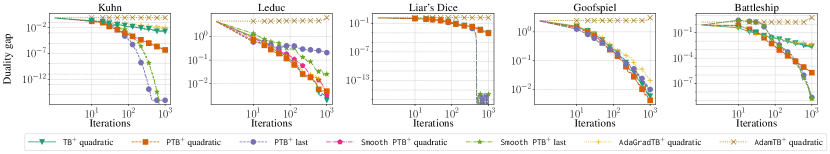
Figure 4: Convergence to Nash equilibrium as a function of number of iterations for TB⁺ with quadratic averaging, PTB⁺ with quadratic averaging and last iterate, and Smooth PTB⁺ with quadratic averaging and last iterate. Every algorithm is using alternation.

I.4 Individual Performance

In Figures 5 to 12, we compare the individual performance of TB⁺, PTB⁺, Smooth PTB⁺, AdaGradTB⁺, AdamTB⁺, CFR⁺, PCFR⁺ and SC-POMD with different weighting schemes, with and without alternation. We also show the performance of the last iterate. The goal is to choose the most favorable framework for each algorithms, in order to have a fair comparison. We find that all algorithms benefit from using alternation. CFR⁺ enjoys stronger performance using linear weights, whereas PTB⁺, PCFR⁺ and SC-POMD have stronger performances with quadratic weights. For this reason this is the setup that we present for comparing the performance of these algorithms in our main body (Figure 2).

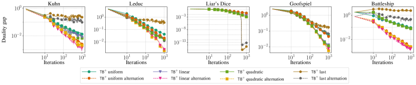
Figure 5: Convergence to Nash equilibrium as a function of number of iterations using uniform, linear, and quadratic averaging, as well as the last iterate, with and without alternation for TB⁺.

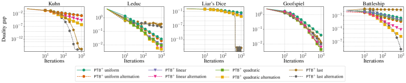
Figure 6: Convergence to Nash equilibrium as a function of number of iterations using uniform, linear, and quadratic averaging, as well as the last iterate, with and without alternation for PTB⁺.

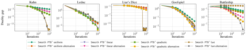
Figure 7: Convergence to Nash equilibrium as a function of number of iterations using uniform, linear, and quadratic averaging, as well as the last iterate, with and without alternation for Smooth PTB⁺.

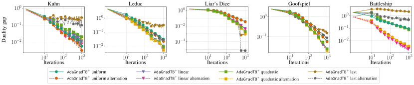
Figure 8: Convergence to Nash equilibrium as a function of number of iterations using uniform, linear, and quadratic averaging, as well as the last iterate, with and without alternation for AdaGradTB⁺.

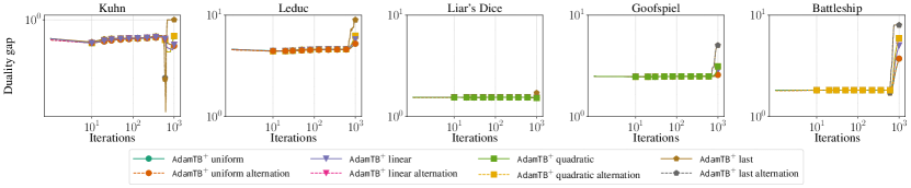
Figure 9: Convergence to Nash equilibrium as a function of number of iterations using uniform, linear, and quadratic averaging, as well as the last iterate, with and without alternation for AdaGradTB⁺.

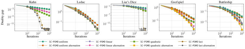
Figure 12: Convergence to Nash equilibrium as a function of number of iterations using uniform, linear, and quadratic averaging, as well as the last iterate, with and without alternation for SC-POMD.

References

• Abernethy etย al. [2011] Jacob Abernethy, Peterย L Bartlett, and Elad Hazan. Blackwell approachability and no-regret learning are equivalent. In Proceedings of the 24th Annual Conference on Learning Theory, pages 27โ€“46. JMLR Workshop and Conference Proceedings, 2011.
• Blackwell [1956] David Blackwell. An analog of the minimax theorem for vector payoffs. Pacific Journal of Mathematics, 6(1):1โ€“8, 1956.
• Brown and Sandholm [2018] Noam Brown and Tuomas Sandholm. Superhuman AI for heads-up no-limit poker: Libratus beats top professionals. Science, 359(6374):418โ€“424, 2018.
• Brown and Sandholm [2019] Noam Brown and Tuomas Sandholm. Superhuman AI for multiplayer poker. Science, 365(6456):885โ€“890, 2019.
• Brown etย al. [2017] Noam Brown, Christian Kroer, and Tuomas Sandholm. Dynamic thresholding and pruning for regret minimization. In Proceedings of the AAAI conference on artificial intelligence, volumeย 31, 2017.
• Burch etย al. [2019] Neil Burch, Matej Moravcik, and Martin Schmid. Revisiting CFR+ and alternating updates. Journal of Artificial Intelligence Research, 64:429โ€“443, 2019.
• Chakrabarti etย al. [2023] Darshan Chakrabarti, Jelena Diakonikolas, and Christian Kroer. Block-coordinate methods and restarting for solving extensive-form games. In Thirty-seventh Conference on Neural Information Processing Systems, 2023.
• Dโ€™Orazio and Huang [2021] Ryan Dโ€™Orazio and Ruitong Huang. Optimistic and adaptive lagrangian hedging. In Thirty-fifth AAAI conference on artificial intelligence, 2021.
• Duchi etย al. [2011] John Duchi, Elad Hazan, and Yoram Singer. Adaptive subgradient methods for online learning and stochastic optimization. Journal of machine learning research, 12(7), 2011.
• Farina etย al. [2019a] Gabriele Farina, Christian Kroer, and Tuomas Sandholm. Online convex optimization for sequential decision processes and extensive-form games. In Proceedings of the AAAI Conference on Artificial Intelligence, volumeย 33, pages 1917โ€“1925, 2019a.
• Farina etย al. [2019b] Gabriele Farina, Christian Kroer, and Tuomas Sandholm. Optimistic regret minimization for extensive-form games via dilated distance-generating functions. In Advances in Neural Information Processing Systems, pages 5222โ€“5232, 2019b.
• Farina etย al. [2021a] Gabriele Farina, Christian Kroer, and Tuomas Sandholm. Better regularization for sequential decision spaces fast convergence rates for Nash, correlated, and team equilibria. In ECโ€™21: Proceedings of the 22nd ACM Conference on Economics and Computation, 2021a.
• Farina etย al. [2021b] Gabriele Farina, Christian Kroer, and Tuomas Sandholm. Faster game solving via predictive Blackwell approachability: Connecting regret matching and mirror descent. In Proceedings of the AAAI Conference on Artificial Intelligence. AAAI, 2021b.
• Farina etย al. [2022] Gabriele Farina, Ioannis Anagnostides, Haipeng Luo, Chung-Wei Lee, Christian Kroer, and Tuomas Sandholm. Near-optimal no-regret learning dynamics for general convex games. Advances in Neural Information Processing Systems, 35:39076โ€“39089, 2022.
• Farina etย al. [2023] Gabriele Farina, Julien Grand-Clรฉment, Christian Kroer, Chung-Wei Lee, and Haipeng Luo. Regret matching+: (in)stability and fast convergence in games. In Advances in Neural Information Processing Systems, 2023.
• Freund and Schapire [1999] Yoav Freund and Robertย E Schapire. Adaptive game playing using multiplicative weights. Games and Economic Behavior, 29(1-2):79โ€“103, 1999.
• Gilpin etย al. [2012] Andrew Gilpin, Javier Pena, and Tuomas Sandholm. First-order algorithm with convergence for-equilibrium in two-person zero-sum games. Mathematical programming, 133(1-2):279โ€“298, 2012.
• Gordon [2007] Geoffreyย J Gordon. No-regret algorithms for online convex programs. In Advances in Neural Information Processing Systems, pages 489โ€“496. Citeseer, 2007.
• Grand-Clรฉment and Kroer [2023] Julien Grand-Clรฉment and Christian Kroer. Solving optimization problems with Blackwell approachability. Mathematics of Operations Research, 2023.
• Hoda etย al. [2010] Samid Hoda, Andrew Gilpin, Javier Pena, and Tuomas Sandholm. Smoothing techniques for computing Nash equilibria of sequential games. Mathematics of Operations Research, 35(2):494โ€“512, 2010.
• Joulani etย al. [2017] Pooria Joulani, Andrรกs Gyรถrgy, and Csaba Szepesvรกri. A modular analysis of adaptive (non-) convex optimization: Optimism, composite objectives, and variational bounds. In International Conference on Algorithmic Learning Theory, pages 681โ€“720. PMLR, 2017.
• Kingma and Ba [2015] Diederikย P. Kingma and Jimmy Ba. Adam: A method for stochastic optimization. In International Conference on Learning Representations, ICLR, 2015.
• Kroer etย al. [2018] Christian Kroer, Gabriele Farina, and Tuomas Sandholm. Solving large sequential games with the excessive gap technique. In Advances in Neural Information Processing Systems, pages 864โ€“874, 2018.
• Kroer etย al. [2020] Christian Kroer, Kevin Waugh, Fatma Kฤฑlฤฑnรง-Karzan, and Tuomas Sandholm. Faster algorithms for extensive-form game solving via improved smoothing functions. Mathematical Programming, pages 1โ€“33, 2020.
• Lee etย al. [2021] Chung-Wei Lee, Christian Kroer, and Haipeng Luo. Last-iterate convergence in extensive-form games. Advances in Neural Information Processing Systems, 34:14293โ€“14305, 2021.
• Milman [2006] Emanuel Milman. Approachable sets of vector payoffs in stochastic games. Games and Economic Behavior, 56(1):135โ€“147, 2006.
• Moravฤรญk etย al. [2017] Matej Moravฤรญk, Martin Schmid, Neil Burch, Viliam Lisแปณ, Dustin Morrill, Nolan Bard, Trevor Davis, Kevin Waugh, Michael Johanson, and Michael Bowling. Deepstack: Expert-level artificial intelligence in heads-up no-limit poker. Science, 356(6337):508โ€“513, 2017.
• Nemirovski [2004] Arkadi Nemirovski. Prox-method with rate of convergence O(1/t) for variational inequalities with Lipschitz continuous monotone operators and smooth convex-concave saddle point problems. SIAM Journal on Optimization, 15(1):229โ€“251, 2004.
• Nesterov [2005] Yurii Nesterov. Excessive gap technique in nonsmooth convex minimization. SIAM Journal on Optimization, 16(1):235โ€“249, 2005.
• Niazadeh etย al. [2021] Rad Niazadeh, Negin Golrezaei, Joshuaย R Wang, Fransisca Susan, and Ashwinkumar Badanidiyuru. Online learning via offline greedy algorithms: Applications in market design and optimization. In Proceedings of the 22nd ACM Conference on Economics and Computation, pages 737โ€“738, 2021.
• Perchet [2010] Vianney Perchet. Approachability, Calibration and Regret in Games with Partial Observations. PhD thesis, PhD thesis, Universitรฉ Pierre et Marie Curie, 2010.
• Rakhlin and Sridharan [2013] Alexander Rakhlin and Karthik Sridharan. Online learning with predictable sequences. In Conference on Learning Theory, pages 993โ€“1019. PMLR, 2013.
• Reddi etย al. [2018] Sashankย J Reddi, Satyen Kale, and Sanjiv Kumar. On the convergence of Adam and beyond. International Conference on Learning Representations (ICLR), 2018.
• Syrgkanis etย al. [2015] Vasilis Syrgkanis, Alekh Agarwal, Haipeng Luo, and Robertย E Schapire. Fast convergence of regularized learning in games. Advances in Neural Information Processing Systems, 28, 2015.
• Tammelin etย al. [2015] Oskari Tammelin, Neil Burch, Michael Johanson, and Michael Bowling. Solving heads-up limit Texas holdโ€™em. In Twenty-Fourth International Joint Conference on Artificial Intelligence, 2015.
• vonย Stengel [1996] Bernhard vonย Stengel. Efficient computation of behavior strategies. Games and Economic Behavior, 14(2):220โ€“246, 1996.
• Zinkevich etย al. [2007] Martin Zinkevich, Michael Johanson, Michael Bowling, and Carmelo Piccione. Regret minimization in games with incomplete information. In Advances in neural information processing systems, pages 1729โ€“1736, 2007.