Differentiable master equation solver for quantum device characterisation

Abstract

Differentiable models of physical systems provide a powerful platform for gradient-based algorithms, with particular impact on parameter estimation and optimal control. Quantum systems present a particular challenge for such characterisation and control, owing to their inherently stochastic nature and sensitivity to environmental parameters. To address this challenge, we present a versatile differentiable quantum master equation solver, and incorporate this solver into a framework for device characterisation. Our approach utilises gradient-based optimisation and Bayesian inference to provide estimates and uncertainties in quantum device parameters. To showcase our approach, we consider steady state charge transport through electrostatically defined quantum dots. Using simulated data, we demonstrate efficient estimation of parameters for a single quantum dot, and model selection as well as the capability of our solver to compute time evolution for a double quantum dot system. Our differentiable solver stands to widen the impact of physics-aware machine learning algorithms on quantum devices for characterisation and control.

I Introduction

The challenge of characterising quantum devices has inspired a myriad of approaches, with the goal of furthering the understanding and application of quantum technologies gebhart2023learning . The simplest approach to characterising aspects of a quantum system is phenomenological fitting, which can yield useful parameter values with minimal resources and carefully selected measurements. More complex methods such as quantum state tomography leonhardt1995quantum and quantum process tomography mohseni2008quantum facilitate full characterisation of the states prepared in a device or how they are changed by device operation, but often require large amounts of data as well as access to observables providing a full tomographic basis set. Several approaches have been developed to improve the efficiency of these tomographic techniques, or to extend their descriptive power, by having appropriate models incorporated into the characterisation of both closed cole2005identifying ; devitt2006scheme ; zhang2014quantum and open quantum systems jorgensen2019exploiting ; white2022non .

Deep learning methods have recently opened many promising avenues for characterising quantum systems. For instance, efficient tomographic methods have been developed using deep learning models as a variational ansatz torlai2018neural , and deep learning methods have also been applied to characterisation of open quantum system dynamics and estimating physical parameters describing the system and environment banchi2018modelling ; hartmann2019neural ; flurin2020using ; barr2023spectral . Learning an abstracted generator of quantum dynamics, such as in the case of deep learning, may lead to accurate prediction of a quantum system’s evolution but often fails to provide direct insight into physical parameters describing the system. Capitalising on prior knowledge about the dominant physical interactions allows for more explicit and efficient characterisation of quantum systems than abstracted tomographic models and with greater flexibility than phenomenological fitting kurchin2024using . In such a physically motivated paradigm, parameter values for a physical model could be inferred from available measurements, and other aspects of the system could be probed by inserting inferred values into the same model.

The success of modern deep learning methods is underpinned by differentiable programming. This programming paradigm facilitates the automatic differentiation required for training deep neural networks with many parameters, where numerical and symbolic derivatives become severely impractical rumelhart1986learning ; baydin2018automatic . Beyond applications to deep learning, differentiable programming has recently been applied to physical models in the context of physics-aware machine learning craig2024bridging ; pachalieva2022physics ; wright2022deep , efficient computation of gradients with respect to complex physical models liao2019differentiable ; Hu2020DiffTaichi: , and optimisation of non-equilibrium steady states vargas2021fully . There have also been recent advances in using differentiable models for simulations of quantum systems with a focus on optimal control schafer2020differentiable ; coopmans2021protocol ; khait2022optimal ; coopmans2022optimal ; sauvage2022optimal .

In this article we apply the concepts of differentiable programming to develop a versatile, fast and differentiable quantum master equation solver. We apply our solver to electrostatically defined quantum dots as they offer a multi-faceted platform for realising quantum systems for which accurate parameter estimation would benefit experiments in quantum computation hanson2007spins ; burkard2023semiconductor ; chatterjee2021semiconductor , quantum thermodynamics josefsson2018quantum , and environment-assisted transport granger2012quantum ; hartke2018microwave . The interaction of discrete charge states with fermionic leads and vibrational modes requires an open quantum systems description, for which weak-coupling master equations can be a suitable choice in many experimental device regimes stace2005population ; hartke2018microwave ; hofmann2020phonon . Measurements of (steady state) charge transport in single and double quantum dot systems are often used to estimate characteristics of the system, such as temperature beenakker1991theory ; prance2012single ; borsoi2023shared , energy spectra, foxman1993effects ; kouwenhoven1997electron , and electron-phonon coupling mechanisms hartke2018microwave ; hofmann2020phonon ; sowa2017environment . However, characterisation of electrostatically defined quantum dot devices remains challenging, not least due to the fact that control via voltages applied to gate electrodes introduces an abstraction between experimental control and system parameters ares2021machine ; zwolak2023colloquium ; gebhart2023learning . Further to this abstracted control, disorder frustrates device characterisation by causing variation in the control parameters for devices of the same design craig2024bridging ; chatzikyriakou2022unveiling ; percebois2021deep ; seidler2023tailoring .

To address such demanding situations, our approach combines a differentiable quantum master equation solver with gradient-based optimisation protocols and Bayesian inference, and is designed to handle a mixture of differentiable and non-differentiable parameters to facilitate a range of applications. In addition to gradient-based optimisation of parameters, Markov chain Monte Carlo methods facilitate estimation of posterior distributions from which parameter uncertainties can be obtained.

To demonstrate the power and broad applicability of our approach, we have designed two case studies with different levels of complexity. The first case study of transport through a single quantum dot with an orbital excited state is designed to highlight our approach’s capabilities in handling differentiable and non-differentiable parameters. The second case study of transport through a double quantum dot coupled to a phonon bath is designed to explore characterisation of the environment gullans2018probing ; hofmann2020phonon ; barr2023spectral . In this second case study, we showcase the ability of our algorithm to discriminate between and correctly select from a set of models featuring different phonon spectral densities relating to different device materials and geometries. To quantitatively assess the performance of our approach, these case studies utilise simulated data. A sketch of the differentiable fitting process, which is central to our approach, is shown in Figure 1(a) along with both case study scenarios in (b) and (c), respectively.

This article is structured as follows: First, we discuss our implementation of a differentiable quantum master equation solver in Section II, before discussing the Bayesian formulation of our parameter estimation algorithm in Section III and optimisation of non-differentiable parameters in Section IV. We apply our approach to case studies of single and double quantum dots in Section V and Section VI respectively. Finally, in Section VII we demonstrate the capability of our model to calculate time evolution of a double quantum dot system.

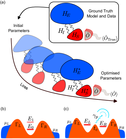
Figure 1: (a) A schematic of the process of estimating parameters of an open quantum system using gradient descent. Here, $H_{\mathrm{S}}$, $H_{\mathrm{E}}$ are the system and environment Hamiltonians, respectively, and $H_{\mathrm{I}}$ is the system-environment interaction Hamiltonian. Expectation values of an observable $\langle\hat{O}\rangle$ are generated from a ground truth model, which would be experimental data in practical applications, and a differentiable model is used to fit these values by gradient descent of a loss function. (b) Representation of the first case study of a single quantum dot with an excited state coupled to left and right leads. Here, $\mu_{\mathrm{L}(\mathrm{R})}$ is the chemical potential of the left(right) lead, $\Gamma_{\mathrm{L}(\mathrm{R})}$ is the tunnel rate between the dot states and the left(right) lead, and $E_{0(1)}$ is the electrochemical potential of the dot in the ground(excited) state. (c) Representation of the second case study of a double quantum dot coupled to left and right leads, and a phonon bath. In each case study the observable used to inform parameter estimation is the steady state current from left to right lead. Here $E_{\mathrm{L}(\mathrm{R})}$ is the chemical potential of the dot with a charge on the left(right) dot, $t_{c}$ is the tunnel coupling between the dots, and $\gamma_{p}$ is the coupling strength to the phonon bath.

II Differentiable Master Equation Solver

The focal point of our quantum device characterisation is a differentiable quantum master equation solver, which is implemented using TensorFlow abadi2016tensorflow . Quantum master equations are a method of determining the time evolution of the system density matrix $\rho$ of an open quantum system breuer2002theory . In a weak-coupling setting this evolution is governed by the Liouvillian superoperator, $\mathcal{L}$, which contains details of both the system Hamiltonian and the system-environment interaction, such that $\dot{\rho}(t)=\mathcal{L}\rho(t)$. A simple manifestation of $\mathcal{L}$ is given by a Lindblad master equation, which reads

$$\dot{\rho}(t)=-i[H_{S},\rho(t)]+\sum_{i}\Gamma_{i}\mathcal{D}[A_{i}]\rho(t),$$ (1)

where $H_{S}$ is the system Hamiltonian, $\Gamma_{i}$ is the dissipation rate associated with the operator $A_{i}$ which describes environment induced transitions in the system, and $\mathcal{D}[A]\rho=A\rho A^{\dagger}-\nicefrac{{1}}{{2}}\{A^{\dagger}A,\rho\}$ is the Lindblad dissipator acting on the density matrix. The dissipation rates are often dependent on system Hamiltonian parameters defining the energy difference between states involved in the environment induced transitions.

Numerically solving such a quantum master equation using differentiable programming facilitates evaluation of the gradient of an observable with respect to the master equation parameters. To compute steady states, we solve the set of linear equations resulting from Eq. (1) under the condition $\dot{\rho}(t)=0$, and for time evolution we use ODE solvers as discussed in Section VII. A differentiable model allows gradients to be obtained with similar computation time to forward evaluation of the model using automatic differentiation, without the need for inefficient finite-element methods. Our implementation can deal with arbitrary Liouvillian superoperators, and is thus applicable to a range of physical systems. Related work has demonstrated differentiable computation of steady state solutions using JAX jax2018github for quantum heat transfer models vargas2021fully . Our approach differs in implementation, design, and application; we use TensorFlow, provide more general construction of Lindblad master equations, and embed our solver in a data-driven device characterisation algorithm.

Using TensorFlow allows direct use of in-built gradient-based optimisation methods such as Adam kingma2014adam , and Bayesian inference methods such as Hamiltonian Monte Carlo (HMC) neal2011mcmc which can be implemented using TensorFlow Probability dillon2017tensorflow . Several differentiable programming libraries, including TensorFlow, have the advantage of allowing vectorised (i.e. batched) inputs and computation performed on a graph which leads to significant speed-up when compared to the same computation performed using a standard library for modelling quantum systems, such as QuTiP johansson2012qutip . Vectorised inputs refer to having the input to the differentiable model be an $n_{\mathrm{b}}\times n_{\theta}$ array for $n_{\theta}$ parameters and a batch of $n_{\mathrm{b}}$ different sets of parameter values, so that the output will be a $n_{\mathrm{b}}\times n_{\mathrm{out}}$ array, where $n_{\mathrm{out}}$ is the number of outputs from the model. An example demonstrating the accuracy and speed of our solver is outlined in Appendix A.

III Bayesian Estimation of Differentiable Parameters

Our approach aims to fit model predictions to data by estimating values for parameters in quantum master equations. We consider case studies of transport through a single quantum dot with an orbital excited state, and through a double quantum dot coupled to a phonon bath. For both the single and double quantum dot case studies, the source-drain bias $V_{\mathrm{bias}}$ and a single 1D current scan are used to inform the parameter estimation. Not all parameters in a model may be differentiable as discussed below, and others may have minimal impact on a loss function so gradients become ineffective. We shall present our approach for dealing with such parameters in general terms before presenting results for each case study.

We denote the $n_{\mathrm{c}}$ parameters which are controlled to produce a batch of $n_{\mathrm{b}}$ data points as $\bm{\theta}^{\mathrm{c}}$, and the remaining $n_{\mathrm{v}}$ parameters under consideration for estimation as $\bm{\theta}^{\mathrm{v}}$. The ground truth data is then $D\!=\!\{d_{j}|j=1\ldots n_{\mathrm{b}}\}$ where $d_{j}$ is an individual data point, and the total set of $n_{\theta}=n_{\mathrm{c}}+n_{\mathrm{v}}$ parameters is $\bm{\theta}=[\bm{\theta}^{\mathrm{c}},\bm{\theta}^{\mathrm{v}}]$. We assume that the ground truth data $D$ is described by a function of the true parameters $f(\bm{\theta}_{\mathrm{true}})$ with Gaussian noise of standard deviation $\sigma$ such that each point in $D$ is $d_{j}\!\sim\!\mathcal{N}(f(\bm{\theta}_{\mathrm{true}}),\sigma)$. Under this assumption we formulate the likelihood of the data given a set of parameters $\bm{\theta}^{\mathrm{v}}$ used to estimate the function $\hat{d}=f(\bm{\theta}^{\mathrm{v}})$ over the domain of $\bm{\theta}^{\mathrm{c}}$ as

$$P(D|\bm{\theta}^{\mathrm{v}})\propto\exp{\Bigg{(}-\frac{\sum_{j=1}^{n_{\mathrm{b}}}(\hat{d}_{j}-d_{j})^{2}}{\sigma^{2}}\Bigg{)}}.$$ (2)

This likelihood can be used in Bayes’ formula $P(\bm{\theta}^{\mathrm{v}}|D)\propto P(D|\bm{\theta}^{\mathrm{v}})P(\bm{\theta}^{\mathrm{v}})$ to estimate the posterior values for parameters in $\bm{\theta}^{\mathrm{v}}$. The prior of each parameter in $\bm{\theta}^{\mathrm{v}}$ can be chosen independently such that $P(\bm{\theta}^{\mathrm{v}})=\prod_{i=1}^{n_{\mathrm{v}}}P(\theta^{\mathrm{v}}_{i})$. The set of parameters which produce the mode of the posterior distribution is the maximum a posteriori (MAP) estimate, and for uniform priors this becomes maximum likelihood estimation (MLE). Evaluation of the negative log probability of the posterior distribution can be used as a differentiable loss function for the gradient descent portion of the parameter fitting process discussed in the previous section. The parameters which minimise this loss correspond to the MAP estimate.

Further to this, a Bayesian approach allows the use of Markov-chain Monte Carlo (MCMC) methods to estimate the posterior distribution for each parameter. We specifically consider Hamiltonian Monte Carlo (HMC) implemented in TensorFlow Probability dillon2017tensorflow to generate a set of $n_{s}$ posterior samples for the parameter values $S=\{\bm{\theta}^{\mathrm{v}}_{j}|j=1\ldots n_{s}\}$, using the MAP estimate as a seed to reduce burn-in. These posterior samples allow for an estimate of uncertainty and correlations in the parameter values. The posterior distribution can also be normalised and used to update the prior distribution for use with further data.

IV Optimising Non-Differentiable Parameters

The output of a model is a function of the parameters, $f(\bm{\theta})$, which may not be differentiable with respect to certain elements of $\bm{\theta}$. In the case of current traces in electrostatically defined quantum dots, such parameters are the definition of the bias window in $\bm{\theta}^{\mathrm{c}}$ due to the abstraction between gate voltages and the energy of the dot electrochemical potential relative to the lead chemical potentials. In other situations, $f(\bm{\theta})$ may not have well-defined gradients across the whole parameter space, which renders gradient descent methods impractical.

To deal with a mixture of differentiable and non-differentiable parameters, we design an optimisation procedure which takes advantage of the fast differentiable model. The idea is to find the non-differentiable parameters for which the remaining differentiable parameters provide the best fit. A Nelder-Mead optimisation routine nelder1965simplex finds appropriate values for the non-differentiable parameters, where the function being optimised is a fit of the model to ground truth data using the remaining differentiable parameters. This fit first involves a log-spaced grid search of the differentiable elements of $\bm{\theta}^{\mathrm{v}}$ where the evaluation of $f(\bm{\theta})$ with the lowest loss with respect to the ground truth data is selected as a starting point for a short gradient descent optimisation using the Adam optimiser. The evaluation of the function being optimised by the Nelder-Mead routine is simply the final loss after this gradient descent. Finally, using the optimal non-differentiable parameters, conducting a longer gradient descent optimisation of the differentiable parameters provides an estimate of all parameters in $\bm{\theta}$. A schematic of this optimisation procedure is shown in Appendix B.

The model fitting algorithm discussed above is general to the situation when some non-differentiable parameters must be optimised before optimising differentiable parameters. For our case studies, the non-differentiable parameters define the energy scale of the measurement axis, which in turn defines how parameters such as tunnel rates change the profile of the fit. This is a result of dot electrochemical potentials being controlled by gate voltages in experiments, which do not have well defined values relative to the bias window. In other experimental settings, it may be the case that the measurement axis is easily quantifiable (e.g. the frequency of an oscillating signal) and so the order in which differentiable and non-differentiable parameters are optimised becomes less important.

V Case Study: Single Quantum Dot with Orbital Excited State

Model

We model a single quantum dot (SQD) with an orbital excited state as shown in Figure 1(b) such that the set of charge states correspond to a maximum of one excess charge on the dot. This restriction is motivated by the large charging energy of the quantum dot compared to the bias window and the energy splitting between the ground and first orbital excited state. The available charge states are $|0\rangle$, $|G\rangle$, and $|E\rangle$, where $|0\rangle$ has an integer $M$ charges on the dot, $|G\rangle$ and $|E\rangle$ both have $M+1$ charges on the dot. The single excess charge exists in the ground state for $|G\rangle$, and an orbital excited state for $|E\rangle$. The Hamiltonian describing the coupling between these charge states and the leads is given by

$$H =H_{0}+H_{l}+H_{el},$$ (3)

$$H_{0} =E_{0}|G\rangle\langle G|+\big{(}E_{0}+\delta\big{)}|E\rangle\langle E|,$$ (4)

$$H_{l} =\sum_{k}(\epsilon_{k}-\mu_{l})d_{kl}^{\dagger}d_{kl}+(\epsilon_{k}-\mu_{r})d_{kr}^{\dagger}d_{kr},$$ (5)

$$H_{el} =\sum_{k}\sum_{j=g,e}(t_{l}d_{kl}^{\dagger}c_{j}+t_{r}d_{kr}^{\dagger}c_{j}+\mathrm{H.c.}),$$ (6)

where $E_{0}$ is the energy of the ground state, and $\delta$ is the energy splitting between the ground and orbital excited state. $H_{l}$ describes the leads with $\mu_{l(r)}$ being the chemical potential of the left(right) leads, and $d_{kl(r)}^{\dagger}(d_{kl(r)})$ are the fermionic creation(annihilation) operators for the left(right) lead for the mode of energy $\epsilon_{k}$. $H_{el}$ describes the coupling between the dot states and the leads where $c_{g(e)}$ is the fermionic annihilation operator acting on the ground(excited) dot, $t_{l(r)}$ are the tunnel couplings between the leads and the dot states, and H.c. denotes the Hermitian conjugate. For simplicity, we assume the same tunnel rates to the leads for both the ground and excited charge state.

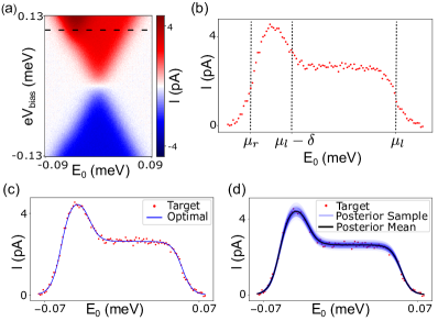
Figure 2: An example of our approach applied to a single quantum dot with an orbital excited state. (a) A Coulomb diamond from which the current trace in (b) is taken, indicated by the black dashed line. (b) The example ground truth simulated current data with $100\ \mathrm{fA}$ Gaussian noise used to fit parameters, with the bias set to $0.109\ \mathrm{mV}$. Nominal locations of the points on the $E_{0}$ axis defined by the non-differentiable parameters $[\mu_{l},\mu_{r},\delta]$ are indicated by vertical dashed lines. (c) The results of gradient descent parameter optimisation on $[\Gamma_{\mathrm{L}},\Gamma_{\mathrm{R}},T]$ after the non-differentiable parameters have been fitted. (d) The HMC posterior samples of the current values generated using 500 posterior samples of the parameters $[\Gamma_{\mathrm{L}},\Gamma_{\mathrm{R}},T]$. Ground truth and optimal parameter values, as well as posterior means with standard deviation errors for relevant parameters, are shown in Table 1.

To model the steady state current flowing through the SQD at a given source-drain bias $V_{\mathrm{bias}}$ we solve a master equation of the form,

$$\dot{\rho}=-i[H_{0},\rho]+\mathcal{L}_{\mathrm{leads}}\rho,$$ (7)

where $\rho$ is the density matrix of the SQD system and $\mathcal{L}_{\mathrm{leads}}$ is the dissipator associated with the leads. In the weak-coupling regime $\mathcal{L}_{\mathrm{leads}}$ takes the form

$$\begin{split}\mathcal{L}_{\mathrm{leads}}=\sum_{j=G,E}&\Big{\{}\big{(}W_{sj}+W_{dj}\big{)}\mathcal{D}[|j\rangle\langle 0|]\ +\\ &\big{(}\overline{W}_{dj}+\overline{W}_{sj}\big{)}\mathcal{D}[|0\rangle\langle j|]\Big{\}}.\end{split}$$ (8)

The tunnel rates from a lead onto the dot are given by $W_{\mathrm{L(R)}j}=\Gamma_{\mathrm{L(R)}}f_{\mathrm{L(R)}}(E_{j})$ and from the dot onto the lead $\overline{W}_{\mathrm{L(R)}j}=\Gamma_{\mathrm{L(R)}}\big{[}1-f_{\mathrm{L(R)}}(\epsilon_{j})\big{]}$, where $\Gamma_{\mathrm{L(R)}}=\pi g_{\mathrm{L(R)}}|t_{l(r)}|^{2}$ with $g_{\mathrm{L(R)}}$ the constant density of states in the leads in the wide band approximation, and $f_{\mathrm{L(R)}}(\epsilon)=[e^{(\epsilon-\mu_{l(r)})/k_{B}T}+1]^{-1}$ is the Fermi-Dirac distribution for the left(right) lead.

With $e$ denoting the electronic charge and $\rho_{\mathrm{ss}}$ the steady state solution of Eq. (7), the steady state current flowing though the SQD is

$$I=e\sum_{j=E,G}\overline{W}_{j\mathrm{R}}\mathrm{Tr}(\rho_{\mathrm{ss}}|j\rangle\langle j|)-W_{j\mathrm{R}}\mathrm{Tr}(\rho_{\mathrm{ss}}|0\rangle\langle 0|).$$ (9)

Parameter Estimation

We consider the model presented above as a case study to assess the performance of each part of the parameter estimation process. This model has a single controlled parameter $\bm{\theta}^{\mathrm{c}}=[E_{0}]$ which is swept through the bias window. The variable parameters $\bm{\theta}^{\mathrm{v}}=[\mu_{l},\mu_{r},\delta,\Gamma_{\mathrm{L}},\Gamma_{\mathrm{R}},T]$ can be separated into differentiable parameters $[\Gamma_{\mathrm{L}},\Gamma_{\mathrm{R}},T]$ and non-differentiable parameters $[\mu_{l},\mu_{r},\delta]$. The left and right chemical potentials are non-differentiable as they define the energy scale of the data before the model is computed, and the orbital excited state energy splitting $\delta$ has zero gradient for large areas of the parameter space and is thus optimised as a non-differentiable parameter.

Parameter	Unit	Ground Truth	Optimal	Posterior Mean $\pm$ Std.
$\mu_{l}$	pixels	15.4	15.3	-
$\mu_{r}$	pixels	96.6	96.4	-
$\delta$	meV	0.084	0.085	-
$\Gamma_{\mathrm{L}}$	MHz	18.1	18.0	18.4 $\pm$ 0.8
$\Gamma_{\mathrm{R}}$	MHz	183.1	180.6	171.3 $\pm$ 4.3
$T$	mK	55.9	53.4	59.4 $\pm$ 1.8

Table 1: Ground truth, optimal, and posterior means with standard deviation errors for the example shown in Figure 2. The non-differentiable parameters are not part of the HMC sampling and therefore do not have posterior means and uncertainties.

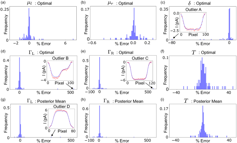
Figure 3: Distributions of percentage errors for parameter estimation over a test set of 100 randomly generated current traces for a single quantum dot with an orbital excited state. Distributions displayed are: (a)-(c) optimal values of non-differentiable parameters $[\mu_{l},\mu_{r},\delta]$, (d)-(f) optimal values of differentiable parameters $[\Gamma_{\mathrm{L}},\Gamma_{\mathrm{R}},T]$, and (g)-(i) posterior means for the differentiable parameters. All distributions are peaked at zero error, with a small number of outliers. Insets show the target data (red points) and optimal fit (blue line) for selected outliers.

An example of our parameter estimation algorithm is shown in Figure 2 with parameter estimates shown in Table 1. In this example, the largest absolute percentage error in optimised non-differentiable values is 1.2%, and in optimal differentiable values is 4.5%. Posterior means and standard deviations drift slightly from the optimal parameter values, but retain a good fit to the data. In Figure 3 we consider the distributions of percentage errors for each parameter for a set of 100 iterations of our parameter estimation algorithm on randomly generated data. The distributions are all peaked at zero percentage error, indicating that our parameter estimation method is generally effective. There are a small number of outliers with large errors, but upon further inspection we find that most of these outliers have no discernible second peak in the current profile (see insets of Figure 3, specifically Outliers A, C, and D). This means the location of the excited state cannot be determined at the first optimisation step, which impacts the estimation of further parameters. The outliers have a lower signal to noise ratio than typical samples which may further impact the parameter estimation, as evident in Outlier B which does have an excited state peak. From Figure 3, we observe that parameter estimate using the posterior mean from HMC samples has a more narrow distribution around zero percentage error, and is therefore generally better than the gradient descent optimal values.

VI Case Study: Double Quantum Dot

Model

The second case study considers a double quantum dot (DQD) coupled to left and right leads and a phonon bath, as shown in Figure 1(c). The states describing the DQD are $|0\rangle$, $|L\rangle$, and $|R\rangle$ where $|0\rangle$ has $(M,N)$ charges on the dot, $|L\rangle$ has $(M+1,N)$ charges, and $|R\rangle$ has $(M,N+1)$ charges. The Hamiltonian describing the coupling between these charge states, the leads, and the phonon bath is given by

$$H =H_{0}+H_{l}+H_{p}+H_{el}+H_{ep},$$ (10)

$$H_{0} =\frac{\epsilon}{2}\sigma_{z}+t_{c}\sigma_{x},$$ (11)

$$H_{l} =\sum_{k}(\epsilon_{k}-\mu_{l})d_{kl}^{\dagger}d_{kl}+(\epsilon_{k}-\mu_{r})d_{kr}^{\dagger}d_{kr},$$ (12)

$$H_{p} =\sum_{\mathbf{k}}\omega_{\mathbf{k}}a_{\mathbf{k}}^{\dagger}a_{\mathbf{k}},$$ (13)

$$H_{el} =\sum_{k}(t_{l}d_{kl}^{\dagger}c_{l}+t_{r}d_{kr}^{\dagger}c_{r}+\mathrm{H.c.}),$$ (14)

$$H_{ep} =\sigma_{z}\sum_{\mathbf{k}}\lambda_{\mathbf{k}}(a_{\mathbf{k}}^{\dagger}+a_{\mathbf{k}}),$$ (15)

where $\sigma_{\mu}$ are the Pauli operators in the subspace $|L\rangle$ and $|R\rangle$, $\epsilon=E_{\mathrm{L}}-E_{\mathrm{R}}$ is the detuning between the dot energy levels, and $t_{c}$ is the interdot tunnel rate. $H_{l}$ describes the leads with $\mu_{l(r)}$ being the chemical potential of the left(right) leads, and $d_{kl(r)}^{\dagger}(d_{kl(r)})$ are the fermionic creation(annihilation) operators for the left(right) lead for the mode of energy $\epsilon_{k}$. $H_{el}$ describes the coupling between the dots and the leads where $c_{l(r)}$ is the fermionic annihilation operator acting on the left(right) dot, and $t_{l(r)}$ are the tunnel couplings between the leads and the dots. The phonon bath is described by $H_{p}$ where $a_{\mathbf{k}}^{\dagger}(a_{\mathbf{k}})$ are the creation(annihilation) operators for the phonon mode of angular frequency $\omega_{\mathbf{k}}$. The electron-phonon interaction is described by $H_{ep}$ where $\lambda_{\mathbf{k}}$ is the coupling constant between the dots and the phonons.

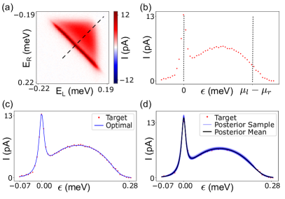
Figure 4: An example of our approach applied to a double quantum dot coupled to a phonon bath. (a) A bias triangle from which the current trace in (b) is taken, indicated by the black dashed line. (b) The example ground truth simulated current data with $100\ \mathrm{fA}$ Gaussian noise used to fit parameters, with the bias set to $0.241\ \mathrm{mV}$. Nominal locations of the points on the $E_{0}$ axis defined by the non-differentiable parameters $[\mu_{l},\mu_{r}]$ are indicated by vertical dashed lines. (c) The results of gradient descent parameter optimisation on $[\Gamma_{\mathrm{L}},\Gamma_{\mathrm{R}},t_{c},J_{0},T]$ after the non-differentiable parameters have been fitted. (d) The HMC posterior samples of the current values generated using 500 posterior samples of the parameters $[\Gamma_{\mathrm{L}},\Gamma_{\mathrm{R}},t_{c},J_{0},T]$. This example considers a 3-dimensional piezoelectric phonon spectral density with fixed parameters are $c_{s}=3000\ \mathrm{ms}^{-1}$, $a=20\ \mathrm{nm}$, and $d=100\ \mathrm{nm}$. Ground truth and optimal parameter values, as well as posterior means with standard deviation errors for relevant parameters, are shown in Table 2.

To model the steady state current flowing through the DQD at a given source-drain bias $V_{\mathrm{bias}}=\mu_{l}-\mu_{r}$ we solve a master equation of the form

$$\dot{\rho}=-i[H_{0},\rho]+\mathcal{L}_{\mathrm{leads}}\rho+\mathcal{L}_{\mathrm{phonons}}\rho,$$ (16)

where $\rho$ is the density matrix of the DQD system, and $\mathcal{L}_{\mathrm{leads}}$ and $\mathcal{L}_{\mathrm{phonons}}$ are the dissipators associated with the leads and phonon bath, respectively. In the weak-coupling regime $\mathcal{L}_{\mathrm{leads}}$ takes the form

$$\begin{split}\mathcal{L}_{\mathrm{leads}}=&W_{\mathrm{L}}\mathcal{D}[|L\rangle\langle 0|]+\overline{W}_{\mathrm{L}}\mathcal{D}[|0\rangle\langle L|]+\\ &W_{\mathrm{R}}\mathcal{D}[|R\rangle\langle 0|]+\overline{W}_{\mathrm{R}}\mathcal{D}[|0\rangle\langle R|],\end{split}$$ (17)

where the tunnel rates from a lead onto its neighbouring dot follow equivalent definitions as for the previous case study.

The phonon dissipator is most conveniently expressed in terms of the eigenstates of $H_{0}$, which for positive detuning are

$$|+\rangle =\cos(\nicefrac{{\theta}}{{2}})|L\rangle-\sin(\nicefrac{{\theta}}{{2}})|R\rangle,$$ (18)

$$|-\rangle =\sin(\nicefrac{{\theta}}{{2}})|L\rangle+\cos(\nicefrac{{\theta}}{{2}})|R\rangle,$$ (19)

with energy $\hbar\omega_{\pm}\!=\!\pm\sqrt{\epsilon^{2}/4+t_{c}^{2}}$. The energy splitting between the eigenstates is $\hbar\omega_{p}\!=\!\hbar(\omega_{+}-\omega_{-})$, and $\theta=\arctan(2t_{c}/\epsilon)$. The weak-coupling phonon dissipator stace2005population is then,

$$\begin{split}\mathcal{L}_{\mathrm{phonons}}=\gamma(\omega_{p})&\big{(}[1+n(\omega_{p})]\mathcal{D}[|-\rangle\langle+|]\\ &+n(\omega_{p})\mathcal{D}[|+\rangle\langle-|]\big{)},\end{split}$$ (20)

where $\gamma(\omega)\!=\!\sin^{2}{\theta}J(\omega)$ is the rate at which the phonon bath induces interdot charge transitions in the DQD, dictated by the phonon spectral density

$$J(\omega)=2\pi\sum_{\mathbf{k}}|\lambda_{\mathbf{k}}|^{2}\delta(\omega-\omega_{\mathbf{k}}).$$ (21)

The functional form of the phonon spectral density can be modelled as

$$J(\omega)=J_{0}\bigg{(}\frac{\omega}{\omega_{d}}\bigg{)}^{n-\alpha}\bigg{[}1-\operatorname{sinc}{\bigg{(}\frac{\omega}{\omega_{d}}\bigg{)}}\bigg{]}e^{-\omega^{2}/2\omega_{a}^{2}},$$ (22)

where $\omega_{d}=\frac{2\pi c}{d}$ and $\omega_{a}=\frac{2\pi c}{a}$, with $d$ the centre-to-centre separation of the dots, $a$ the linear extent of the dots, and $c$ the speed of sound in the crystal, and $J_{0}$ is a scale factor. We also have $n$ as the dimension of the system, and $\alpha=0$ for piezoelectric coupling and $\alpha=2$ for deformation potential coupling to phonons. The complete set of spectral densities for varying dimensions and coupling mechanism is shown in Appendix D.

The Bose-Einstein occupation of the phonon bath $n(\omega)=[e^{\omega/k_{B}T}-1]^{-1}$ produces a temperature dependence on the phonon emission and absorption processes that are described by $\mathcal{D}[|-\rangle\langle+|]$ and $\mathcal{D}[|+\rangle\langle-|]$, respectively. As the DQD system is at low temperature ($k_{B}T\!\ll\!\omega_{p}$), phonon emission processes dominate.

With $e$ denoting the electronic charge, using the steady state solution of Eq. (16), $\rho_{\mathrm{ss}}$, the steady state current flowing though the DQD is

$$I=e\big{[}\overline{W}_{\mathrm{R}}\mathrm{Tr}(\rho_{\mathrm{ss}}|R\rangle\langle R|)-W_{\mathrm{R}}\mathrm{Tr}(\rho_{\mathrm{ss}}|0\rangle\langle 0|)\big{]}.$$ (23)

Model Selection

We now consider the model presented above to assess the performance of our approach on a more complex system. This model has a single controlled parameter $\bm{\theta}^{\mathrm{c}}=[\epsilon]$ which is varied such that each dot energy level is swept through the bias window. We choose the variable parameters to be $\bm{\theta}^{\mathrm{v}}=[\mu_{l},\mu_{r},\Gamma_{\mathrm{L}},\Gamma_{\mathrm{R}},t_{c},J_{0},T]$ which can be separated into differentiable parameters $[\Gamma_{\mathrm{L}},\Gamma_{\mathrm{R}},t_{c},J_{0},T]$ and non-differentiable parameters $[\epsilon_{0},\epsilon_{\mathrm{bias}}]$ which are the points where $\epsilon=0$ and $\epsilon=\mu_{\mathrm{L}}-\mu_{\mathrm{R}}$, respectively. The remaining parameters are set to representative fixed values of $c_{s}=3000\ \mathrm{ms}^{-1}$, $a=20\ \mathrm{nm}$, and $d=100\ \mathrm{nm}$. We choose these parameters to be fixed as they can all be estimated from the device design, but they could also be included in the set of differentiable parameters. The dot radius $a$ in particular has minimal impact on the fit for the energy scales probed by typical experimental measurements. The problem of estimating parameters for this model from a single current trace is expected to be underdetermined due to the number of parameters defining the system. We find fitting to data points is accurate, with an example shown in Figure 4. Discussion of parameter estimation for this model can be found in Appendix C.

Capitalising on the accuracy of fitting to data, we use our approach to characterise other aspects of a device hosting these dots. We focus on model selection for the interaction of the double quantum dot with phonons, using our fitting process to perform model selection on the phonon spectral density. The phonon spectral density is determined by material properties and dimensionality of the semiconductor in which the dots are defined, as well as the geometry of the dots, as outlined in Appendix D. Accurately distinguishing between piezoelectric and deformation potential phonon coupling would yield information about the device in which the dots are formed. Determining the dimensionality of the phonon spectral density would yield information about the confinement of phonon modes in the device and help identify any possible waveguide effects.

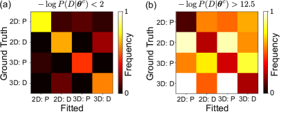
Figure 5: The occurrence of fits which have a negative log likelihood of (a) less than 2, and (b) greater than 12.5 in a test set of 50 for each ground truth model. In each ground truth model a different phonon spectral density is used, with ‘3D: D’ being 3-dimensional deformation potential, ‘3D: P’ 3-dimensional piezoelectric, ‘2D: D’ 2-dimensional deformation potential, and ‘2D: P’ 2-dimensional piezoelectric. With Gaussian noise, $-\log{P(D|\bm{\theta}^{\mathrm{c}})}<2$ indicates that the average error is less than 2 noise standard deviations from the ground truth which we consider to be a good fit. Fits with $-\log{P(D|\bm{\theta}^{\mathrm{c}})}>12.5$ indicates that the average error is more than 5 noise standard deviations, representing a failure of fitting. We fit the non-differentiable parameters $[\epsilon_{0},\epsilon_{\mathrm{bias}}]$ and the differentiable parameters $[\Gamma_{\mathrm{L}},\Gamma_{\mathrm{R}},t_{c},J_{0},T]$. Fixed parameters are $c_{s}=3000\mathrm{ms}^{-1}$, $a=20\mathrm{nm}$, and $d=100\mathrm{nm}$.

In Figure 5 we present the results of performing our fitting process with each phonon spectral density (2D and 3D deformation potential, 2D and 3D piezoelectric) on datasets with different ground truth spectral densities. We use the negative log likelihood, $-\log{P(D|\bm{\theta}^{\mathrm{c}})}$, as a metric for our fit. As the data has Gaussian noise, the value of the negative log likelihood indicates the number of noise standard deviations a given fit is from the true value. In Figure 5(a) we display the frequency of fits which are within two standard deviations of the true value on average. Having the largest values along the diagonal indicates that our fit is only successful when the correct model is used, providing evidence that the functional form of the spectral density adds a significant constraint on the fit. The failed fits which are on average more than five standard deviations from the true value are shown in Figure 5(b), and in this case the diagonal has the lowest values indicating that the fitting process does not fail often when using the correct model. We can also observe from this plot that the fitting process is notably worse when fitting piezoelectric spectral densities to data with deformation potential spectral densities, and also performs poorly when fitting deformation potential spectral densities to data generated using piezoelectric spectral densities in 3D. Fits which are between 2 and 5 standard deviations of the ground truth could still be classed as successful but may be more subjective, so we do not consider them useful when assessing our fitting of different spectral densities.

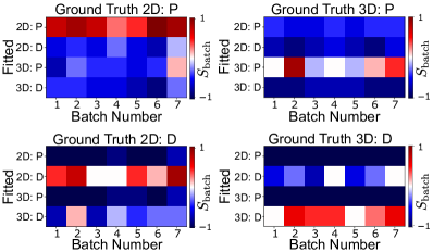
Figure 6: The score of fitting to a batch of size $n_{\mathrm{batch}}=7$ for each phonon spectral density considered in Figure 5. The batch score $S_{\mathrm{batch}}=(n_{\mathrm{success}}-n_{\mathrm{failure}})/n_{\mathrm{batch}}$ for seven independent batches is plotted for each fitted spectral density. A positive score indicates that the spectral density fit succeeds more than it fails within the batch, in accordance to the definitions of success and failure discussed in the text. We see that the best scores for each batch correlate with the ground truth spectral density.

We find that our approach provides useful insight into the electron-phonon coupling mechanism in a double quantum dot system, even when individual model parameters cannot be accurately determined. In order to apply this strategy to real data where the ground truth is not available, using a batch of size $n_{\mathrm{batch}}$ detuning traces from different bias triangles allows a decision to be made when selecting a model based on the frequencies of fit outcomes displayed in Figure 5. Defining a score function $S_{\mathrm{batch}}=(n_{\mathrm{success}}-n_{\mathrm{failure}})/n_{\mathrm{batch}}$ where $n_{\mathrm{success}}$ is the number of fits in a batch with $-\log{P(D|\bm{\theta}^{\mathrm{c}})}<2$ and $n_{\mathrm{failure}}$ is the number of fits in a batch with $-\log{P(D|\bm{\theta}^{\mathrm{c}})}>12.5$ provides reliable insight into the correct phonon coupling mechanism for simulated test data as shown in Figure 6 which considers the case of $n_{\mathrm{batch}}\!=\!7$.

VII Time Evolution

Having considered parameter estimation from steady-state solutions to quantum master equations using our differentiable solver, this section briefly explores time-evolution functionality and its limitations. Dynamic control of qubits is a natural motivation for studying time evolution, and thus we consider the model of a double quantum dot coupled to fermionic leads and a phonon bath outlined above as charge qubits have been implemented in such systems gorman2005charge ; petersson2010quantum . A Lindblad master equation can be recast as a set of coupled ordinary differential equations (ODEs) for time evolution solutions, which means standard ODE solvers can be used. Our solver implements a $4^{\mathrm{th}}$ order Runge-Kutta method butcher2016numerical to compute time-dynamics. To verify that our solver is accurate, Figure 7 shows that the steady state solution is reached after a suitable evolution time under the influence of a time-independent Hamiltonian. This figure also demonstrates batch computation of time-evolution, whereby a batch of $n_{\mathrm{b}}=250$ detuning values is evolved from an initial state of $|\psi(0)\rangle=(|0\rangle+|L\rangle+|R\rangle)/\sqrt{3}$ over 15 ns for 1500 time steps in 0.38s using the same hardware as discussed in Appendix A.

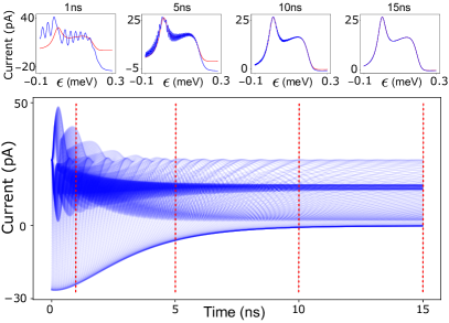
Figure 7: The time-evolution of a double quantum dot system coupled to left and right leads and a phonon bath with a time-independent Hamiltonian. The upper plots display the current as a function of detuning at several points along the evolution, with the steady state current (red) shown for comparison. The evolution is computed as a batch of $n_{\mathrm{b}}=250$ detuning values and evolved for $15\ \mathrm{ns}$ with a step-size of $0.01\ \mathrm{ns}$. The initial state for the entire batch is the pure state, $|\psi(0)\rangle=(|0\rangle+|L\rangle+|R\rangle)/\sqrt{3}$. Parameter values used are, $V_{\mathrm{bias}}=0.2\ \mathrm{mV}$, $\Gamma_{\mathrm{L}}=\Gamma_{\mathrm{R}}=500\ \mathrm{MHz}$, $t_{c}=4\ \mathrm{GHz}$ and $T=100\mathrm{mK}$. The phonon coupling follows a 3D piezoelectric spectral density with $c_{s}=3000\ \mathrm{ms}^{-1}$, $a=20\ \mathrm{nm}$, and $d=50\mathrm{nm}$, and $J_{0}=1\ \mathrm{GHz}$.

In addition to evolution under a time-independent Hamiltonian, our solver can handle time-dependent Hamiltonians. We demonstrate this functionality by considering a Rabi pulse sequence on the DQD system operating as a charge qubit, with the details and results of this pulse sequence shown in Figure 8. We initialise the DQD such that the charge is on the left dot, with its electrochemical potential remaining below the source and drain chemical potentials for the duration of the sequence. The electrochemical potential of the right dot is pulsed by an energy $\delta\epsilon$ for a duration $\tau_{p}$ which defines the Rabi pulse. We then simulate the integration of current for a duration of $\tau_{m}$ and output the mean current during this period. Successfully reproducing the expected charge qubit dynamics under time-independent and time-dependent Hamiltonians is a demonstration that our $4^{\mathrm{th}}$ order Runge-Kutta solver is sufficient for the phenomena considered, however more sophisticated solvers could make computation of dynamics more efficient butcher2016numerical . We note that while batch computation of time evolution is facilitated by our solver, providing a speed improvement over conventional solvers, gradients with respect to pulse parameters would require further work to implement a differentiable model for optimal quantum control.

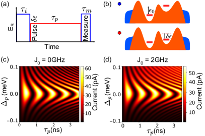
Figure 8: Demonstration of a Rabi pulse sequence on a DQD charge qubit computed using our quantum master equation solver. (a) Outline of the sequence whereby the DQD is initialised to be $|\psi(0)\rangle=|L\rangle$ and after a time $\tau_{i}=1\ \mathrm{ns}$ a pulse is applied to the right dot to vary the detuning by $\delta\epsilon$ for a duration of $\tau_{p}$, and current is measured for a time $\tau_{m}=1\ \mathrm{ns}$. (b) Schematics of the DQD in the initialisation and measurement regime (top and the pulsed regime (bottom). Rabi chevrons without (c) and with (d) coupling to a phonon bath. We define the pulse detuning $\Delta_{p}=|\delta\epsilon|-|\epsilon_{0}|$ and the measured current is taken to be the mean current integrated during the measurement period. Parameter values used are, $\Gamma_{\mathrm{L}}=\Gamma_{\mathrm{R}}=500\ \mathrm{MHz}$, $t_{c}=4\ \mathrm{GHz}$ and $T=100\ \mathrm{mK}$. The phonon coupling follows a 3D piezoelectric spectral density with $c_{s}=3000\ \mathrm{ms}^{-1}$, $a=20\ \mathrm{nm}$, and $d=50\ \mathrm{nm}$, and $J_{0}=1\ \mathrm{GHz}$.

VIII Conclusion

We have presented a fast and differentiable quantum master equation solver, and demonstrated its capability to compute steady state solutions and time evolution of open quantum systems. Our solver can be applied to any system described by a Lindblad master equation, and minimal changes would permit application to a more general time-local approach involving fewer approximations. The speed of our solver comes from its capability to compute a batch of outputs in a single evaluation of a model. This speed in turn facilitates more involved algorithms requiring many evaluations, which would be impractical using standard solvers. An example of such an algorithm is the model fitting approach we develop which employs both gradient-based and gradient-free optimisation, and MCMC methods.

Our parameter estimation algorithm has been applied to case studies of transport through a single quantum dot with an orbital excited state, and a double quantum dot coupled to a phonon bath. We have found our approach to be successful for dealing with parameter estimation in the case of a single quantum dot. To highlight the utility of our algorithm, we have also performed model selection to determine the electron-phonon coupling mechanism in a double quantum dot. Our approach is successful in reliably determining the ground truth spectral density. Our approach could be directly applied to experimental studies of the spectral density, such as in Ref. hofmann2020phonon . Decoherence from electron-phonon interactions impacts both charge and spin qubits, therefore characterising the details of this coupling mechanism is important for understanding qubit dynamics.

Our differentiable master equation solver and its application to parameter estimation is a new approach to characterising quantum systems, and we anticipate similar differentiable models will provide significant utility across a range of applications. Physics-aware machine learning is a notable area in which differentiable models have been applied previously craig2024bridging ; pachalieva2022physics ; wright2022deep , and our solver stands to widen the impact of such approaches. In addition, differentiable pulse simulators have been identified as ‘urgently needed’ in the field of quantum pulse engineering liang2022variational . Our work steps towards reaching this goal in the framework of differentiable programming for quantum master equations, but there remains scope for future work for fully differentiable time evolution.

Code availability

The code used in this work is available online at https://doi.org/10.5281/zenodo.10783608.

Appendix A Differentiable Solver Test Case

To demonstrate the effectiveness of our differentiable solver, we consider the case of a single quantum dot (SQD) coupled to left and right leads. Considering the basis states $|0\rangle$ for $N$ electrons on the dot, and $|1\rangle$ for $N+1$ electrons on the dot, the total Hamiltonian is

$$H =H_{0}+H_{l}+H_{el},$$ (A24)

$$H_{0} =\epsilon|1\rangle\langle 1|,$$ (A25)

$$H_{l} =\sum_{k}(\epsilon_{k}-\mu_{l})d_{kl}^{\dagger}d_{kl}+(\epsilon_{k}-\mu_{r})d_{kr}^{\dagger}d_{kr},$$ (A26)

$$H_{el} =\sum_{k}\sum_{i=l,r}t_{i}(d_{ki}^{\dagger}c+d_{ki}c^{\dagger}),$$ (A27)

where $\epsilon$ is the chemical potential of the dot, $d_{kl(r)}^{\dagger}$ and $d_{kl(r)}$ are the creation and annihilation operators for the $k^{th}$ mode in the left(right) lead, and $t_{l(r)}$ is the tunnel coupling between the dot and modes in the left(right) lead. The operators $c=|0\rangle\langle 1|$ and $c^{\dagger}=|1\rangle\langle 0|$ act on the quantum dot occupation. To model the steady state current flowing through the SQD at a given source-drain bias $V_{\mathrm{bias}}=\mu_{l}-\mu_{r}$ we solve a master equation of the form,

$$\dot{\rho}=\mathcal{L}\rho=-i[H_{0},\rho]+\mathcal{L}_{\mathrm{leads}}\rho,$$ (A28)

where $\rho$ is the density matrix of the SQD system, $\mathcal{L}$ is the Liouvillian superoperator, and $\mathcal{L}_{\mathrm{leads}}$ is the dissipator associated with the leads. In the weak-coupling regime $\mathcal{L}_{\mathrm{leads}}$ takes the form

$$\mathcal{L}_{\mathrm{leads}}\rho=-\big{(}W_{\mathrm{L}}\mathcal{D}[c^{\dagger}]\rho+\overline{W}_{\mathrm{L}}\mathcal{D}[c]\rho+W_{\mathrm{r}}\mathcal{D}[c^{\dagger}]\rho+\overline{W}_{\mathrm{R}}\mathcal{D}[c]\rho\big{)},$$ (A29)

where the Lindblad superoperators act according to $\mathcal{D}[A]\rho=A\rho A^{\dagger}-\nicefrac{{1}}{{2}}\{A^{\dagger}A,\rho\}$. The energy dependent tunnel rates from a lead onto the dot are given by $W_{\mathrm{L(R)}}=\Gamma_{\mathrm{L(R)}}f_{l(r)}(\epsilon)$ and from the dot onto the lead $\overline{W}_{\mathrm{L(R)}}=\Gamma_{\mathrm{L(R)}}\big{[}1-f_{l(r)}(\epsilon)\big{]}$, where $\epsilon$ is the electrochemical potential of the dot and $f_{l(r)}(\epsilon)=[e^{(\epsilon-\mu_{l(r)})/k_{B}T}+1]^{-1}$ is the Fermi-Dirac distribution for the left(right) lead.

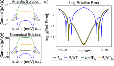
Figure 9: The steady state current and its derivatives using (a) analytic solutions and (b) the differentiable solver. Parameters are set as $\Gamma_{\mathrm{L}}=150\mathrm{Hz}$, $\Gamma_{\mathrm{R}}=200\mathrm{Hz}$, and $T=100\mathrm{mK}$. A quantitative comparison of the numerical outputs and analytic solutions is shown in (c) using the logarithm of the relative absolute error. All plots share the same legend.

With $e$ denoting the electronic charge and $\rho_{\mathrm{ss}}$ the steady state solution of Eq. (A28), the steady state current flowing though the SQD is computed as

$$I_{\mathrm{ss}}=e\big{[}\overline{W}_{\mathrm{R}}\mathrm{Tr}(\rho_{\mathrm{ss}}|1\rangle\langle 1|)-W_{\mathrm{L}}\mathrm{Tr}(\rho_{\mathrm{ss}}|0\rangle\langle 0|)\big{]}.$$ (A30)

This model has the benefit of a simple analytic solution for the steady state current which can be used to directly compare with the output and gradients generated by our solver. The steady state current is

$$I_{\mathrm{ss}}=e\ \frac{W_{\mathrm{L}}\overline{W}_{\mathrm{R}}-\overline{W}_{\mathrm{L}}W_{\mathrm{R}}}{\Gamma_{\mathrm{L}}+\Gamma_{\mathrm{R}}}$$ (A31)

with gradients with respect to $\Gamma_{\mathrm{L}}$, $\Gamma_{\mathrm{R}}$, and $T$ being

$$\frac{\partial I_{\mathrm{ss}}}{\partial\Gamma_{\mathrm{L}}} =\frac{e\Gamma_{\mathrm{R}}^{2}}{(\Gamma_{\mathrm{L}}+\Gamma_{\mathrm{R}})^{2}}\Big{[}f_{l}(\epsilon)-f_{r}(\epsilon)\Big{]},$$ (A32)

$$\frac{\partial I_{\mathrm{ss}}}{\partial\Gamma_{\mathrm{R}}} =\frac{e\Gamma_{\mathrm{L}}^{2}}{(\Gamma_{\mathrm{L}}+\Gamma_{\mathrm{R}})^{2}}\Big{[}f_{l}(\epsilon)-f_{r}(\epsilon)\Big{]},$$ (A33)

$$\frac{\partial I_{\mathrm{ss}}}{\partial T} =\frac{e\Gamma_{\mathrm{L}}\Gamma_{\mathrm{R}}}{\Gamma_{\mathrm{L}}+\Gamma_{\mathrm{R}}}\Big{[}\frac{\partial f_{l}(\epsilon)}{\partial T}-\frac{\partial f_{r}(\epsilon)}{\partial T}\Big{]},$$ (A34)

where

$$\frac{\partial f_{l(r)}(\epsilon)}{\partial T}=\frac{\epsilon-\mu_{l(r)}}{k_{B}T^{2}}\cosh^{-2}{\Big{(}\frac{\epsilon-\mu_{l(r)}}{2k_{B}T}\Big{)}}.$$ (A35)

Values of $I_{\mathrm{ss}}$ and its derivatives computed using the differentiable solver are compared with the analytic results in Figure 9, displaying good agreement in relative error across the domain of dot energy $\epsilon$. We use 32 bit precision for real valued elements of the differentiable solver, with complex values defined using two 32 bit floats.

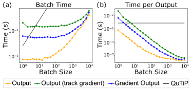
Figure 10: The total time (a) and the time per output (b) for computations on a range of batch sizes using the differentiable master equation for the single quantum dot model described in Eq. (A28). Each point is an average of 100 evaluation times and the time per output is simply the total time divided by the batch size. Output refers to the time taken to compute the output of a batch of input parameters. To compute a gradient by automatic differentiation, a variable must be tracked during the output computation, and once the output is available the gradient can be evaluated. Both plots share the same legend. The black lines corresponding to QuTiP execution times are extrapolated from the time taken for a single computation.

Having established that our differentiable solver returns the desired values, we now investigate the speed of the model and how computation time scales with the batch size, $n_{\mathrm{b}}$. The numerical results presented in Figure 9 were performed by sending a batch of $n_{\mathrm{b}}=200$ parameter values with varying dot energy $\epsilon$ to our solver. We compare the evaluation of the output on the same hardware (Intel(R) Core(TM) i5-9500 CPU) with QuTiP, an established library for solving quantum master equations johansson2012qutip . As shown in Figure 10(a), our differentiable model computes batch outputs significantly faster than QuTiP (where batch computation scales linearly) across all tested batch sizes. Tracking and evaluating gradients adds an overhead to computation time which is much more noticeable at low batch sizes. Considering the computation time per output, Figure 10(b) demonstrates the advantage of batched inputs with our solver where the time per output decreases to less than $10\ \mu s$. These fast computation times make our model ideal for computing a vector of outputs and evaluating the desired gradients.

Appendix B Algorithm Overview

An overview of our approach for dealing with a mixture of differentiable and non-differentiable parameters is shown in Figure 11. We show the order of operation used for the case studies discussed in the main text. After an exploratory log-spaced grid search, the optimisation of non-differentiable parameters uses a Nelder-Mead optimiser to minimise the loss from optimisation of the differentiable parameters using the given non-differentiable parameters. The final step is to perform a longer optimisation of differentiable parameter using the optimised non-differentiable parameters.

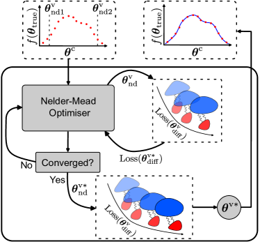
Figure 11: A schematic of our approach for optimising differentiable and non-differentiable parameters when fitting to data. The example shown is purely illustrative and does not contain real data. Here, we denote non-differentiable parameters as $\bm{\theta}^{\mathrm{v}}_{\mathrm{nd}}$ and differentiable parameters as $\bm{\theta}^{\mathrm{v}}_{\mathrm{diff}}$. Sets of optimised parameters are indicated with an asterisk. Optimisation of differentiable parameters is indicated by the schematic introduced in Figure 1 (a).

Appendix C Double Quantum Dot Parameter Estimation

Table 2 displays the parameter estimation results for the example shown in Figure 4. The bias is set to $0.241\ \mathrm{mV}$, and the remaining parameters are set to representative fixed values of $c_{s}=3000\ \mathrm{ms}^{-1}$, $a=20\ \mathrm{nm}$, and $d=100\ \mathrm{nm}$. The performance of this example is representative of our approach’s parameter estimation for this model.

The combination of an accurate fit and inaccurate parameter estimates indicate that this problem is underdetermined using the available data, as expected. To improve the performance of parameter estimation additional data would be required to constrain the fit. An example of such additional data could be a current scan along the base of the bias triangle, perpendicular to the detuning scan shown in Figure 4. Our Bayesian formulation then allows for posterior distributions of values for parameters from one fit to be used as priors for the subsequent fit.

Parameter	Unit	Ground Truth	Optimal	Posterior Mean $\pm$ Std.
$\epsilon_{0}$	pixels	10.4	10.3	-
$\epsilon_{\mathrm{bias}}$	pixels	45.5	45.6	-
$\Gamma_{\mathrm{L}}$	MHz	854.1	127.0	126.2 $\pm$ 5.4
$\Gamma_{\mathrm{R}}$	MHz	166.4	529.5	540.9 $\pm$ 38.2
$t_{c}$	GHz	1.49	0.91	0.94 $\pm$ 0.04
$J_{0}$	GHz	0.98	3.18	2.96 $\pm$ 0.3
$T$	mK	143.7	136.5	126.1 $\pm$ 24.7

Table 2: Ground truth, optimal, and posterior means with standard deviation errors for the example shown in Figure 4. The non-differentiable parameters are not part of the HMC sampling and therefore do not have posterior means and uncertainties.

Appendix D Spectral Densities

The following discussion provides a brief derivation of the spectral density functions considered in this article. In a spin-boson model such as that described by $H_{sb}=H_{0}+H_{p}+H_{ep}$, and assuming the bosonic environment is in thermal equilibrium, the environment is completely described by the spectral density function $J(\omega)=2\pi\sum_{\mathbf{k}}|\lambda_{\mathbf{k}}|^{2}\delta(\omega-\omega_{\mathbf{k}})$ as defined in (21).

	Phonon Spectral Density: $J(\omega)$
Dimension	Deformation Potential	Piezoelectric
3D	$\frac{D^{2}\hbar}{2\pi^{2}\mu c^{2}d^{3}}\ \Big{(}\frac{\omega}{\omega_{d}}\Big{)}^{3}\ \Big{(}1-\operatorname{sinc}{\frac{\omega}{\omega_{d}}}\Big{)}e^{-\frac{\omega^{2}}{2\omega_{a}^{2}}}$	$\frac{P^{2}\hbar}{2\pi^{2}\mu c^{2}d}\ \frac{\omega}{\omega_{d}}\ \Big{(}1-\operatorname{sinc}{\frac{\omega}{\omega_{d}}}\Big{)}e^{-\frac{\omega^{2}}{2\omega_{a}^{2}}}$
2D	$\frac{D^{2}\hbar}{4\pi^{2}\mu c^{2}d^{2}}\ \Big{(}\frac{\omega}{\omega_{d}}\Big{)}^{2}\ \Big{[}1-J_{0}\Big{(}\frac{\omega}{\omega_{d}}\Big{)}\Big{]}e^{-\frac{\omega^{2}}{2\omega_{a}^{2}}}$	$\frac{P^{2}\hbar}{4\pi^{2}\mu c^{2}}\ \Big{[}1-J_{0}\Big{(}\frac{\omega}{\omega_{d}}\Big{)}\Big{]}e^{-\frac{\omega^{2}}{2\omega_{a}^{2}}}$
1D	$\frac{D^{2}\hbar}{8\pi^{3}\mu c^{2}d}\ \frac{\omega}{\omega_{d}}\ \Big{(}1-\cos{\frac{\omega}{\omega_{d}}}\Big{)}e^{-\frac{\omega^{2}}{2\omega_{a}^{2}}}$	$\frac{P^{2}\hbar d}{8\pi^{3}\mu c^{2}}\ \frac{\omega_{d}}{\omega}\ \Big{(}1-\cos{\frac{\omega}{\omega_{d}}}\Big{)}e^{-\frac{\omega^{2}}{2\omega_{a}^{2}}}$

Table 3: A summary of the phonon spectral density functions for deformation potential and piezoelectric interactions with a double quantum dot in varying dimensions. A similar table of spectral densities can be found in Ref. stace2005population .

The interaction Hamiltonian $H_{ep}$ has a diagonal ($\sigma_{z}$) system operator by considering well defined quantum dots with minimal overlap of the dot wavefunctions, i.e. $\langle L|R\rangle\!\ll\!1$. Using the single particle wavefunctions, the phonon coupling matrix element $\lambda_{\mathbf{k}}$ is defined as,

$$\begin{split}\lambda_{\mathbf{k}}&=M_{\mathbf{k}}\big{(}\langle L|e^{i\mathbf{k}\cdot\mathbf{r}}|L\rangle-\langle R|e^{i\mathbf{k}\cdot\mathbf{r}}|R\rangle\big{)}\\ &=M_{\mathbf{k}}\int\!d\mathbf{r}\big{[}\psi_{L}(\mathbf{r})-\psi_{R}(\mathbf{r})\big{]}e^{i\mathbf{k}\cdot\mathbf{r}}\end{split}$$ (D36)

where $M_{\mathbf{k}}$ is a matrix element which depends on the material properties of the system.

Adopting the notation $\mathbf{k}=(\bm{\kappa},k_{z})$ and $\mathbf{r}=(\bm{\rho},r_{z})$, and assuming the dots exist in the x-y plane with identical, radially symmetric wavefunctions separated by a vector $\mathbf{d}$ such that $\psi_{L}(\bm{\rho},r_{z})\!=\!\psi(\bm{\rho},r_{z})$ $\psi_{R}(\bm{\rho},r_{z})\!=\!\psi(\bm{\rho}-\mathbf{d},r_{z})$ it follows that

$$\lambda_{\mathbf{k}}=M_{\mathbf{k}}\big{(}1-e^{i\bm{\kappa}\cdot\bm{\rho}}\big{)}|\tilde{\psi}(\bm{\kappa},k_{z})|^{2}.$$ (D37)

Substituting this result into (21) we can derive the form factor for the spectral density $J(\omega)$. We use a linear dispersion relation, $\omega_{k}\!=\!c_{s}|\mathbf{k}|\!=\!c_{s}k$ where $c_{s}$ is the speed of sound in the crystal, and omit the prefactor $M_{\mathbf{k}}$ to find the angular form factor, $F(\omega)$, based on the dot geometry,

$$F(\omega)=\sum_{\mathbf{k}}\delta(\omega-ck)|\tilde{\psi}(\kappa,k_{z})|^{4}|1-e^{i\kappa\cdot\mathbf{d}}|^{2}.$$ (D38)

We convert the sum over wavevectors to a 3D integral, $\sum_{\mathbf{k}}\!\to\!\frac{v}{(2\pi)^{3}}\int d\mathbf{k}$. Using the Jacobi-Anger expansion and performing the radial and azimuthal integrals, it follows that

$$\begin{split}F(\omega)=\frac{v\omega^{2}}{2\pi^{2}c_{s}^{3}}\int_{0}^{\pi}&|\tilde{\psi}\Big{(}\frac{\omega}{c_{s}}\sin{\theta},\frac{\omega}{c_{s}}\cos{\theta}\Big{)}|^{4}\times\\ &[1-J_{0}\Big{(}\frac{\omega d}{c_{s}}\sin{\theta}\Big{)}]\sin{\theta}d\theta,\end{split}$$ (D39)

where $J_{0}(\cdot)$ is the zeroth order Bessel function of the first kind. Changing variables to $x\!=\!\cos{\theta}$ we have,

$$\begin{split}F(\omega)=\frac{v\omega^{2}}{\pi^{2}c_{s}^{3}}\int_{0}^{1}&\Big{|}\tilde{\psi}\Big{(}\frac{\omega}{c_{s}}\sqrt{1-x^{2}},\frac{\omega}{c_{s}}x\Big{)}\Big{|}^{4}\times\\ &\Big{[}1-J_{0}\Big{(}\frac{\omega d}{c_{s}}\sqrt{1-x^{2}}\Big{)}\Big{]}dx.\end{split}$$ (D40)

Assuming a sharply peaked electron density simplifies the integral as $|\tilde{\psi}(\bm{\kappa},k_{z})|^{4}\approx 1$. In the context of a double quantum dot system this is a reasonable assumption as the dots are usually confined to a narrow region of space in all directions. The finite extent of the dot wavefunctions, assumed to be Gaussian $\psi(\mathbf{r})\propto e^{-r^{2}/2a^{2}}$, introduces a Gaussian decay from the Fourier transform of the dot wavefunction in D37.

Finally, we make use of the integral $\int_{0}^{z}J_{0}(\sqrt{z^{2}-x^{2}})dx=\sin{z}$ to evaluate the angular form factor of the spectral density,

$$F(\omega)=\frac{v}{\pi^{2}cd^{2}}\bigg{(}\frac{\omega}{\omega_{d}}\bigg{)}^{2}\bigg{(}1-\operatorname{sinc}{\frac{\omega}{\omega_{d}}}\bigg{)}e^{-\omega^{2}/2\omega_{a}^{2}},$$ (D41)

where $\omega_{d}=c_{s}/d$ and $\omega_{a}=c_{s}/a$. A similar derivation can be performed in 2D and 1D by reducing the dimensionality of the angular integral.

The prefactor $M_{\mathbf{k}}$ depends on the type of phonon interaction mahan2000many . The total interaction matrix element is the sum of deformation potential and piezoelectric interaction,

$$M_{\mathbf{k}}=\bigg{(}\frac{1}{2M\omega_{\mathbf{k}}}\bigg{)}^{-1/2}(D|\mathbf{k}|+iP),$$ (D42)

where M is the average mass of the unit cell, and $D$ and $P$ are the deformation potential and piezoelectric constants. Being out of phase, the contributions do not interfere to second order. The form of the respective spectral densities in (22) follows directly from these results. A summary of the functional forms of the spectral densities for deformation potential and piezoelectric phonon coupling with a double quantum dot in varying dimensions is shown in Table 3.

References

- (1) Gebhart, V. et al. Learning quantum systems. Nature Reviews Physics 5, 141–156 (2023).
- (2) Leonhardt, U. Quantum-state tomography and discrete wigner function. Physical Review Letters 74, 4101 (1995).
- (3) Mohseni, M., Rezakhani, A. T. & Lidar, D. A. Quantum-process tomography: Resource analysis of different strategies. Physical Review A 77, 032322 (2008).
- (4) Cole, J. H. et al. Identifying an experimental two-state hamiltonian to arbitrary accuracy. Physical Review A 71, 062312 (2005).
- (5) Devitt, S. J., Cole, J. H. & Hollenberg, L. C. Scheme for direct measurement of a general two-qubit hamiltonian. Physical Review A 73, 052317 (2006).
- (6) Zhang, J. & Sarovar, M. Quantum hamiltonian identification from measurement time traces. Physical Review Letters 113, 080401 (2014).
- (7) Jørgensen, M. R. & Pollock, F. A. Exploiting the causal tensor network structure of quantum processes to efficiently simulate non-markovian path integrals. Physical Review Letters 123, 240602 (2019).
- (8) White, G. A., Pollock, F. A., Hollenberg, L. C., Modi, K. & Hill, C. D. Non-markovian quantum process tomography. PRX Quantum 3, 020344 (2022).
- (9) Torlai, G. et al. Neural-network quantum state tomography. Nature Physics 14, 447–450 (2018).
- (10) Banchi, L., Grant, E., Rocchetto, A. & Severini, S. Modelling non-markovian quantum processes with recurrent neural networks. New Journal of Physics 20, 123030 (2018).
- (11) Hartmann, M. J. & Carleo, G. Neural-network approach to dissipative quantum many-body dynamics. Physical Review Letters 122, 250502 (2019).
- (12) Flurin, E., Martin, L. S., Hacohen-Gourgy, S. & Siddiqi, I. Using a recurrent neural network to reconstruct quantum dynamics of a superconducting qubit from physical observations. Physical Review X 10, 011006 (2020).
- (13) Barr, J., Zicari, G., Ferraro, A. & Paternostro, M. Spectral density classification for environment spectroscopy. arXiv preprint arXiv:2308.00831 (2023).
- (14) Kurchin, R. C. Using bayesian parameter estimation to learn more from data without black boxes. Nature Reviews Physics 1–3 (2024).
- (15) Rumelhart, D. E., Hinton, G. E. & Williams, R. J. Learning representations by back-propagating errors. Nature 323, 533–536 (1986).
- (16) Baydin, A. G., Pearlmutter, B. A., Radul, A. A. & Siskind, J. M. Automatic differentiation in machine learning: a survey. Journal of Marchine Learning Research 18, 1–43 (2018).
- (17) Craig, D. L. et al. Bridging the reality gap in quantum devices with physics-aware machine learning. Physical Review X 14, 011001 (2024).
- (18) Pachalieva, A., O’Malley, D., Harp, D. R. & Viswanathan, H. Physics-informed machine learning with differentiable programming for heterogeneous underground reservoir pressure management. Scientific Reports 12, 18734 (2022).
- (19) Wright, L. G. et al. Deep physical neural networks trained with backpropagation. Nature 601, 549–555 (2022).
- (20) Liao, H.-J., Liu, J.-G., Wang, L. & Xiang, T. Differentiable programming tensor networks. Physical Review X 9, 031041 (2019).
- (21) Hu, Y. et al. Difftaichi: Differentiable programming for physical simulation. In International Conference on Learning Representations (2020).
- (22) Vargas-Hernández, R. A., Chen, R. T., Jung, K. A. & Brumer, P. Fully differentiable optimization protocols for non-equilibrium steady states. New Journal of Physics 23, 123006 (2021).
- (23) Schäfer, F., Kloc, M., Bruder, C. & Lörch, N. A differentiable programming method for quantum control. Machine Learning: Science and Technology 1, 035009 (2020).
- (24) Coopmans, L., Luo, D., Kells, G., Clark, B. K. & Carrasquilla, J. Protocol discovery for the quantum control of majoranas by differentiable programming and natural evolution strategies. PRX Quantum 2, 020332 (2021).
- (25) Khait, I., Carrasquilla, J. & Segal, D. Optimal control of quantum thermal machines using machine learning. Physical Review Research 4, L012029 (2022).
- (26) Coopmans, L., Campbell, S., De Chiara, G. & Kiely, A. Optimal control in disordered quantum systems. Physical Review Research 4, 043138 (2022).
- (27) Sauvage, F. & Mintert, F. Optimal control of families of quantum gates. Physical Review Letters 129, 050507 (2022).
- (28) Hanson, R., Kouwenhoven, L. P., Petta, J. R., Tarucha, S. & Vandersypen, L. M. Spins in few-electron quantum dots. Reviews of Modern Physics 79, 1217 (2007).
- (29) Burkard, G., Ladd, T. D., Pan, A., Nichol, J. M. & Petta, J. R. Semiconductor spin qubits. Reviews of Modern Physics 95, 025003 (2023).
- (30) Chatterjee, A. et al. Semiconductor qubits in practice. Nature Reviews Physics 3, 157–177 (2021).
- (31) Josefsson, M. et al. A quantum-dot heat engine operating close to the thermodynamic efficiency limits. Nature Nanotechnology 13, 920–924 (2018).
- (32) Granger, G. et al. Quantum interference and phonon-mediated back-action in lateral quantum-dot circuits. Nature Physics 8, 522–527 (2012).
- (33) Hartke, T., Liu, Y.-Y., Gullans, M. & Petta, J. Microwave detection of electron-phonon interactions in a cavity-coupled double quantum dot. Physical Review Letters 120, 097701 (2018).
- (34) Stace, T., Doherty, A. & Barrett, S. Population inversion of a driven two-level system in a structureless bath. Physical Review Letters 95, 106801 (2005).
- (35) Hofmann, A. et al. Phonon spectral density in a gaas/algaas double quantum dot. Physical Review Research 2, 033230 (2020).
- (36) Beenakker, C. W. Theory of coulomb-blockade oscillations in the conductance of a quantum dot. Physical Review B 44, 1646 (1991).
- (37) Prance, J. et al. Single-shot measurement of triplet-singlet relaxation in a si/sige double quantum dot. Physical Review Letters 108, 046808 (2012).
- (38) Borsoi, F. et al. Shared control of a 16 semiconductor quantum dot crossbar array. Nature Nanotechnology 1–7 (2023).
- (39) Foxman, E. et al. Effects of quantum levels on transport through a coulomb island. Physical Review B 47, 10020 (1993).
- (40) Kouwenhoven, L. P. et al. Electron transport in quantum dots. Mesoscopic Electron Transport 105–214 (1997).
- (41) Sowa, J. K., Mol, J. A., Briggs, G. A. D. & Gauger, E. M. Environment-assisted quantum transport through single-molecule junctions. Physical Chemistry Chemical Physics 19, 29534–29539 (2017).
- (42) Ares, N. Machine learning as an enabler of qubit scalability. Nature Reviews Materials 6, 870–871 (2021).
- (43) Zwolak, J. P. & Taylor, J. M. Colloquium: Advances in automation of quantum dot devices control. Reviews of Modern Physics 95, 011006 (2023).
- (44) Chatzikyriakou, E. et al. Unveiling the charge distribution of a gaas-based nanoelectronic device: A large experimental dataset approach. Physical Review Research 4, 043163 (2022).
- (45) Percebois, G. J. & Weinmann, D. Deep neural networks for inverse problems in mesoscopic physics: Characterization of the disorder configuration from quantum transport properties. Physical Review B 104, 075422 (2021).
- (46) Seidler, I. et al. Tailoring potentials by simulation-aided design of gate layouts for spin-qubit applications. Phys. Rev. Appl. 20, 044058 (2023).
- (47) Gullans, M., Taylor, J. & Petta, J. R. Probing electron-phonon interactions in the charge-photon dynamics of cavity-coupled double quantum dots. Physical Review B 97, 035305 (2018).
- (48) Abadi, M. et al. Tensorflow: Large-scale machine learning on heterogeneous distributed systems. arXiv preprint arXiv:1603.04467 (2016).
- (49) Breuer, H.-P. & Petruccione, F. The theory of open quantum systems (Oxford University Press, USA, 2002).
- (50) Bradbury, J. et al. JAX: composable transformations of Python+NumPy programs (2018). URL http://github.com/google/jax.
- (51) Kingma, D. P. & Ba, J. Adam: A method for stochastic optimization. arXiv preprint arXiv:1412.6980 (2014).
- (52) Neal, R. M. et al. Mcmc using hamiltonian dynamics. Handbook of Markov chain Monte Carlo 2, 2 (2011).
- (53) Dillon, J. V. et al. Tensorflow distributions. arXiv preprint arXiv:1711.10604 (2017).
- (54) Johansson, J. R., Nation, P. D. & Nori, F. Qutip: An open-source python framework for the dynamics of open quantum systems. Computer Physics Communications 183, 1760–1772 (2012).
- (55) Nelder, J. A. & Mead, R. A simplex method for function minimization. The Computer Journal 7, 308–313 (1965).
- (56) Gorman, J., Hasko, D. & Williams, D. Charge-qubit operation of an isolated double quantum dot. Physical Review Letters 95, 090502 (2005).
- (57) Petersson, K., Petta, J., Lu, H. & Gossard, A. Quantum coherence in a one-electron semiconductor charge qubit. Physical Review Letters 105, 246804 (2010).
- (58) Butcher, J. C. Numerical methods for ordinary differential equations (John Wiley & Sons, 2016).
- (59) Liang, Z. et al. Variational quantum pulse learning. In 2022 IEEE International Conference on Quantum Computing and Engineering (QCE), 556–565 (IEEE, 2022).
- (60) Mahan, G. D. Many-particle physics (Springer Science & Business Media, 2000).