Resurgent Wilson loops in refined topological string

Abstract

We study the resurgent structures of Wilson loops in refined topological string theory. We argue that the Borel singularities should be integral periods, and that the associated Stokes constants are refined Donaldson-Thomas invariants, just like the free energies, except that the Borel singularities cannot be local flat coordinates. We also solve the non-perturbative series in closed form from the holomorphic anomaly equations for the refined Wilson loops. We illustrate these results with the examples of local $\mathbb{P}^{2}$ and local $\mathbb{P}^{1}\times\mathbb{P}^{1}$.

1 Introduction

It is now a general agreement that most asymptotic series in physics are in want of a non-perturbative completion. Topological string theory as a subsector of type II superstring theory compactified on Calabi-Yau threefolds has many asymptotic series, which are both mathematically well-defined and more amenable to calculations, and it is therefore a perfect laboratory to explore non-perturbative completions of asymptotic series. In general, the non-perturbative completion would be ambiguous. However, under the assumption that the asymptotic series in topological string is resurgent, the non-perturbative corrections are strongly constrained, and the powerful method of resurgence theory Ecalle can be used to study them.

According to the resurgence theory, the non-perturbative corrections to an asymptotic series of Gevrey-1 type

$$\varphi(z)=\sum_{n}\varphi_{n}z^{n},\quad\varphi_{n}\sim n!$$ (1.1)

can be encoded in a trans-series of the form

$$\varphi^{(*)}={\rm e}^{-\mathcal{A}_{*}/z}\sum_{n}\varphi^{(*)}_{n}z^{n+b_{*}}.$$ (1.2)

Furthermore, these trans-series are closedly related to the perturbative series via Stokes transformations, so that much information of the trans-series can be extracted from the perturbative series $\varphi$. For instance, the non-perturbative action $\mathcal{A}_{*}$ that determines the magnitude ${\rm e}^{-\mathcal{A}_{*}/z}$ of the non-perturbative correction is given as singularities of the Borel transform of the asymptotic series, while the coefficients in the non-perturbative corrections, together with the coefficients of the Stokes transformations known as the Stokes constants, can be read off from the large order asymptotics of the perturbative coefficients. These data are sometimes collectively called the resurgent structure.

The resurgence method was first applied to study the perturbative free energy $F(t;g_{s})$ in topological string Marino:2006hs ; Marino:2007te ; Marino:2008ya ; Marino2009 ; Pasquetti2010 as an asymptotic series in the string coupling constant $g_{s}$, and a rich structure of non-perturbative corrections was discovered.

First of all, it was found that the non-perturbative actions or the Borel singularities are integral periods of the mirror Calabi-Yau threefolds Drukker:2011zy ; Aniceto2012 ; Couso-Santamaria2016 ; Couso-Santamaria2015 ; Gu:2023mgf , which are the central charges of D-brane bound states in the type II superstring theory, corresponding to D6-D4-D2-D0 bound states in type IIA superstring or equivalently to D5-D3-D1-D(-1) bound states in type IIB superstring, giving the first hint that the non-perturbative corrections in topological string are related to D-branes.

Secondly, it was postulated and verified in Couso-Santamaria2016 ; Couso-Santamaria2015 ; Couso-Santamaria2017a that the non-perturbative trans-series are constrained by the holomorphic anomaly equations Bershadsky:1993ta ; Bershadsky:1993cx , the same set of partial differential equations that constrains the perturbative free energies. This idea was later further developed and exploited to full extent, and the full non-perturbative trans-series in any non-perturbative sector was solved in closed form Gu:2022sqc ; Gu:2023mgf .

Finally, important progress have been made regarding the Stokes constants. Although their exact calculation is still out of reach in generic scenarios, there has been accumulating evidence Bridgeland:2016nqw ; Bridgeland:2017vbr ; Alim:2021mhp ; Gu:2021ize ; Gu:2023wum ; Iwaki:2023rst that the Stokes constant associated to each non-perturbative sector is the Donaldson-Thomas invariant, the counting of stable bound states of D-branes. It also elucidates further the nature of non-perturbative actions: they are not only D-brane central charges, but the central charges of stable D-brane configurations.

Recently, these progress have been generalised Alexandrov:2023wdj (see also Alim:2022oll ; Grassi:2022zuk ) to refined free energies in topological string $F(t;\epsilon_{1},\epsilon_{2})$. The refined free energy is treated as an asymptotic series in $g_{s}$ denoted as $F(t,\mathsf{b};g_{s})$, where the parameters of Omega background $\epsilon_{1},\epsilon_{2}$ are related to $g_{s}$ via

$$\epsilon_{1}={\mathsf{i}}\mathsf{b}g_{s},\quad\epsilon_{2}=-{\mathsf{i}}\mathsf{b}^{-1}g_{s},$$ (1.3)

with the fixed parameter $\mathsf{b}$, and it returns to the unrefined free energy in the limit $\mathsf{b}\rightarrow 1$. For the refined free energy $F(t,\mathsf{b};g_{s})$, it was found that each non-perturbative sector with action $\mathcal{A}$ splits to two whose actions are $\mathcal{A}/\mathsf{b}$ and $\mathcal{A}\,\mathsf{b}$. The trans-series in such a non-perturbative sector was also written down in closed form Alexandrov:2023wdj , as a trans-series solution to the refined version of the holomorphic anomaly equations Huang:2010kf . Finally, it was argued that in this case, the Stokes constants can be identified with the motivic or refined DT invariants.

In this paper, we would like to study the non-perturbative corrections of another important computable in refined topological string theory, the Wilson loops. They play the role of eigenvalues in the quantum mirror curvse Aganagic:2011mi in the Nekrasov-Shatashvili limit of the refined topological string, and they are encoded in the $qq$-character in the generic Omega background Nekrasov:2015wsu . Topological string on a local Calabi-Yau threefold engineers a 5d $N=1$ SCFT, and when the latter has a gauge theory phase, the Wilson loops are naturally defined. The notion of Wilson loops was extended to topological string on generic local Calabi-Yau threefolds Kim:2021gyj as insertion of additional non-compact 2-cycles, and furthermore, holomorphic anomaly equations for the generalised Wilson loops were written down in Huang:2022hdo ; Wang:2023zcb .

The resurgent structures of refined Wilson loops in the Nekrasov-Shatashvili limit were discussed in Gu:2022fss . The NS Wilson loops in different representations are proportional to each other Huang:2022hdo , and one only needs to study those in the fundamental representation. The generic refined Wilson loops in different representations are very different, and their resurgent structures could potentially be very rich.

We follow the idea of Grassi:2022zuk ; Alexandrov:2023wdj , and treat the perturbative refined Wilson loops, which have similar expansions as refined free energies in terms of the Omega deformation parameters $\epsilon_{1},\epsilon_{2}$, as aymptotic series in $g_{s}$ with fixed deformation parameter $\mathsf{b}$, which turn out also to be of Gevrey-1 type, so that the resurgence theory can be used to study the non-perturbative corrections. We find that rather than studying the Wilson loops in different representations, it is more beneficial to consider the generating series of Wilson loops in all representations, which can be regarded as the free energy of the topological string on a new threefold with insertion of additional non-compact two-cycles in the original Calabi-Yau threefold. Although a rigorous mathematical formulation is still lacking, the similarity with the topological string free energy strongly implies that the resurgent structures of the two are also similar. Indeed, we find that for refined Wilson loops, the non-perturbative actions are also integral periods, with the caveat that they cannot be local flat coordinates (i.e. A-periods); the non-perturbative series can be solved in closed form from holomorphic anomaly equations for Wilson loops; the Stokes constants must be the same as those of refined free energy, and therefore they are also identified with refined DT invariants.

The rest of the paper is structured as follows. We review the resurgent structure of free energy of refined topological string in Section 2, the definition and the calculation of perturbative Wilson loops in Section 3. We present our results of the resurgent structures of Wilson loops in Section 4. We show how to reduce to the unrefined limit and the NS limit in Section 4.2, and we are able to reproduce the results in Gu:2022fss and in particular prove some empirical observations, especially the one that the Stokes constants of NS Wilson loops and those of NS free energies were identical, when the former were not vanishing. Two examples of local $\mathbb{P}^{2}$ and local $\mathbb{P}^{1}\times\mathbb{P}^{1}$ are given in Sections 4.3 and 4.4.

2 Free energies and non-perturbative corrections

2.1 Perturbative refined free energy

The refined topologial string theory is defined over the complexified Kahler moduli space of Calabi-Yau threefold $X$ in the A-model, or the complex structure moduli space of the mirror Calabi-Yau threefold $X^{\vee}$ in the B-model. The perturbative free energy of refined topological string theory is a formal power series in terms of two expansion parameter $\epsilon_{1},\epsilon_{2}$ Huang:2010kf

$$\mathcal{F}(\bm{t};\epsilon_{1},\epsilon_{2})=\sum_{n,g\geq 0}(\epsilon_{1}+\epsilon_{2})^{2n}(\epsilon_{1}\epsilon_{2})^{g-1}\mathcal{F}^{(n,g)}(\bm{t}).$$ (2.1)

The coefficients $\mathcal{F}^{(n,g)}(\bm{t})$ are sections of certain line bundles of the moduli space, parametrised by flat coordinates $\bm{t}$.

There are various ways to compute the coefficients of the refined free energy, including instanton calculus Nekrasov:2002qd , refined topological vertex Iqbal:2007ii , and blowup equations Huang:2017mis (see also Grassi:2016nnt and (Gu:2017ccq, , Sec. 8)). But for our purpose, it is more suitable to use the refined holomorphic anomaly equations (refined HAE) Huang:2010kf , as it generates directly the coefficients of the perturbative series, and in addition, it is applicable over the entire moduli space.

In the framework of refined HAE, it is necessary to extend the free energies $\mathcal{F}^{(n,g)}(\bm{t})$ to non-holomorphic functions $F^{(n,g)}$, and the failure of the holomorphicity is described by the refined HAE. The non-holomorphic functions $F^{(n,g)}$ obtained from the refined HAE reduce to $\mathcal{F}^{(n,g)}$ in appropriate holomorphic limits, which is equivalent to taking a local patch of the associated line bundle, where $\bm{t}$ are the flat coordinates on that local patch. We follow the convention in Gu:2022sqc ; Gu:2023mgf that we use Roman capital letters for the non-holomorphic quantities obtained from HAE, and curly captical letters for their holomorphic limit. Note the prepotential $F^{(0,0)}=\mathcal{F}^{(0,0)}=\mathcal{F}_{0}$ is always holomorphic.

To explain the refined HAE, we need to introduce a few properties of the moduli space $\mathcal{M}$. The moduli space is Kahler, so that the metric is expressed in terms of a Kahler potential, i.e.

$$G_{a\bar{b}}=\partial_{a}\partial_{\bar{b}}K,$$ (2.2)

where $\partial_{a}=\partial_{z^{a}}$ and the $z^{a}$ are a set of global complex coordinates over the moduli space. A set of covariant derivatives $D_{a}$ can then be introduced with the Levi-Civita connection,

$$\Gamma^{a}_{bc}=G^{a\bar{d}}\partial_{b}G_{c\bar{d}}.$$ (2.3)

In addition, the moduli space is special Kahler (see e.g. klemm2018b for more details of the special geometry.), in the sense that in any local path of the moduli space, one can find a symplectic basis – known as a choice of frame – of local flat coordinates as well as their conjugates,

$$\left\{t^{a},\quad\frac{\partial\mathcal{F}_{0}}{\partial t^{a}}\right\},\quad a=1,\ldots,\frac{1}{2}\dim\mathcal{M},$$ (2.4)

both of which are classical periods of the mirror Calabi-Yau threefold $X^{\vee}$, and they are related to each other via the preptential $\mathcal{F}_{0}=\mathcal{F}^{(0,0)}$. We can then introduce the Yukawa coupling

$$C_{abc}(\bm{z})=\frac{\partial t^{\ell}}{\partial z^{a}}\frac{\partial t^{m}}{\partial z^{b}}\frac{\partial t^{n}}{\partial z^{c}}\cdot\frac{\partial}{\partial t^{\ell}}\frac{\partial}{\partial t^{m}}\frac{\partial}{\partial t^{n}}\mathcal{F}_{0}$$ (2.5)

which, despite its definition, is independent of the choice of frame, and is usually a rational function of $\bm{z}$. We also introduce the propagators $S^{ab}$ defined by

$$\partial_{\bar{c}}S^{ab}={\rm e}^{2K}G^{a\bar{d}}G^{b\bar{e}}\overline{C}_{\bar{c}\bar{d}\bar{e}}.$$ (2.6)

which encode the non-holomorphic dependence. The non-holomorphic free energies $F^{(n,g)}$ are functions of both $z^{a},S^{ab}$.

The refined topological string free energies then satisfy an infinitely set of partial differential equations known as the refined HAE Huang:2010kf ,

$$\frac{\partial F^{(n,g)}}{\partial S^{ab}}=\frac{1}{2}\left(D_{a}D_{b}F^{(n,g-1)}+\sideset{}{{}^{\prime}}{\sum}_{n^{\prime},g^{\prime}\geq 0}D_{a}F^{(n^{\prime},g^{\prime})}D_{b}F^{(n-n^{\prime},g-g^{\prime})}\right),\quad n+g>2,$$ (2.7)

where $\sum{}^{\prime}$ means excluding $(n^{\prime},g^{\prime})=(0,0)$ or $(n,g)$. These infinitely many equations can be encoded in a single master equation

$$\frac{\partial}{\partial S^{ab}}\widetilde{Z}=\frac{\epsilon_{1}\epsilon_{2}}{2}D_{a}D_{b}\widetilde{Z},$$ (2.8)

with the partition function

$$\widetilde{Z}=\exp\widetilde{F}=\exp\sum_{n+g>0}(\epsilon_{1}+\epsilon_{2})^{2n}(\epsilon_{1}\epsilon_{2})^{g-1}F^{(n,g)}.$$ (2.9)

These equations are supplemented with the initial conditions that the free energy $F^{(0,1)}$ is related to the propagator by

$$\partial_{a}F^{(0,1)}=\frac{1}{2}C_{abc}S^{bc}+f_{a}(\bm{z})$$ (2.10)

while $F^{(1,0)}$ is given by

$$F^{(1,0)}=-\frac{1}{24}\log(f(\bm{z})\Delta(\bm{z})).$$ (2.11)

Here $f_{a}(\bm{z})$ and $f(\bm{z})$ are model-dependent holomorphic functions of $z^{a}$, and $\Delta(\bm{z})$ is the discriminant, the equation of singular loci in the moduli space.

As the equations (2.7) are recursive in genus $(n,g)$, the free energies $F^{(n,g)}$ can be solved by direct integration up to an integration constant, which is independent of the non-holomorphic propagator $S^{ab}$, and which is purely holomorphic, known as the holomorphic ambiguity. The holomorphic ambiguity is fixed by imposing the boundary conditions that at a conifold singularity of the moduli space, the free energies $\mathcal{F}^{(n,g)}(t_{c})$ in the holomorphic limit with the local flat coordinate $t_{c}$ (appropriately normalised) that vanishes at the singularity satisfy the so-called gap condition Huang:2010kf ; Krefl:2010fm

$$\mathcal{F}(t_{c};\epsilon_{1},\epsilon_{2})= \left(-\frac{1}{12}+\frac{1}{24}(\epsilon_{1}+\epsilon_{2})^{2}(\epsilon_{1}\epsilon_{2})^{-1}\right)\log(t_{c})$$

$$+ \frac{1}{\epsilon_{1}\epsilon_{2}}\sum_{n_{1},n_{2}\geq 0}\frac{(2n_{1}+2n_{2}-3)!}{t_{c}^{2n_{1}+2n_{2}-2}}\hat{B}_{2n_{1}}\hat{B}_{2n_{2}}\epsilon_{1}^{2n_{1}}\epsilon_{2}^{2n_{2}}+\mathcal{O}(t_{c}^{0}),$$ (2.12)

where

$$\hat{B}_{n}=(1-2^{1-n})\frac{B_{n}}{n!}$$ (2.13)

and $B_{n}$ denoting the Bernoulli numbers, and that the free energies are regular everywhere else .

Another important universal feature of the refined free energy is that near the large radius point Hollowood:2003cv ; Huang:2010kf , it has the integrality structure

$$\mathcal{F}(\bm{t};\epsilon_{1,2})=\sum_{w\geq 1}\sum_{\gamma\in H_{2}(X,\mathbb{Z})}\sum_{j_{L,R}}(-1)^{2j_{L}+2j_{R}}N^{\gamma}_{j_{L},j_{R}}\frac{\chi_{j_{L}}(q_{L}^{w})\chi_{j_{R}}(q_{R}^{w})}{w(2\sinh\frac{w\epsilon_{1}}{2})(2\sinh\frac{w\epsilon_{2}}{2})}{\rm e}^{-w\gamma\cdot\bm{t}}.$$ (2.14)

generalising the Gopakumar-Vafa formula of unrefined free energy Gopakumar:1998jq . Here $q_{L,R}={\rm e}^{\epsilon_{L,R}}$ and $\epsilon_{L,R}=\frac{1}{2}(\epsilon_{1}\mp\epsilon_{2})$, and $\chi_{j}(q)$ is the character of $su(2)$ of spin $j\in\frac{1}{2}\mathbb{Z}_{\geq 0}$,

$$\chi_{j}(q)=\frac{q^{2j+1}-q^{-2j-1}}{q-q^{-1}}.$$ (2.15)

$N^{\gamma}_{j_{L},j_{R}}$ are non-negative integer numbers, and they count the numbers of stable D2-D0 brane bound states wrapping curve class $\gamma\in H_{2}(X,\mathbb{Z})$ with spins $(j_{L},j_{R})$ in the little group $SU(2)_{L}\times SU(2)_{R}$ in five dimensions, and they are known as the BPS invariants.

2.2 Non-perturbative corrections

It is more convenient to study non-perturbative corrections to asymptotic series with a single expansion parameter. It is therefore suggested in Grassi:2022zuk ; Alexandrov:2023wdj to use the parametrisation

$$\epsilon_{1}={\mathsf{i}}\mathsf{b}g_{s},\quad\epsilon_{2}=-{\mathsf{i}}\mathsf{b}^{-1}g_{s}$$ (2.16)

to convert the refined free energy $F(\epsilon_{1},\epsilon_{2})$ to a univariate power series in terms of the string coupling $g_{s}$,

$$F(\mathsf{b};g_{s})=F({\mathsf{i}}\mathsf{b}g_{s},-{\mathsf{i}}\mathsf{b}^{-1}g_{s})=\sum_{g\geq 0}g_{s}^{2g-2}F_{g}(\mathsf{b}),$$ (2.17)

where the coefficients $F_{g}(\mathsf{b})$ are not only functions of the moduli $\bm{t}$ but also of the deformation parameter $\mathsf{b}$, given by

$$F_{g}(\mathsf{b})=\sum_{n=0}^{g}(-1)^{n}(\mathsf{b}-\mathsf{b}^{-1})^{2n}F^{(n,g-n)}.$$ (2.18)

It is noted then in Alexandrov:2023wdj that the HAE (2.7) can be re-cast as equations of the deformed free energies $F_{g}(\mathsf{b}):=F_{g}(\bm{z},\bm{S},\mathsf{b})$

$$\frac{\partial F_{g}(\mathsf{b})}{\partial S^{ab}}=\frac{1}{2}\left(D_{a}D_{b}F_{g-1}(\mathsf{b})+\sum_{h=1}^{g-1}D_{a}F_{h}(\mathsf{b})D_{b}F_{g-h}(\mathsf{b})\right),\quad g\geq 2.$$ (2.19)

The initial condition is given by

$$F_{1}(\mathsf{b})=F^{(0,1)}-(\mathsf{b}-\mathsf{b}^{-1})^{2}F^{(1,0)}$$ (2.20)

while at conifold points, the boundary condition (2.12) becomes Alexandrov:2023wdj

$$\mathcal{F}_{g}(t_{c},\mathsf{b})=\frac{c_{g}(\mathsf{b})}{t_{c}^{2g-2}}+\mathcal{O}(1),\quad g\geq 2,$$ (2.21)

where the coefficients $c_{g}(\mathsf{b})$ are

$$c_{g}(\mathsf{b})=-(2g-3)!\sum_{m=0}^{g}\widehat{B}_{2m}\widehat{B}_{2g-2m}\mathsf{b}^{2(2m-g)}.$$ (2.22)

This gap condition reduces to the universal conifold behavior of the unrefined topological string Ghoshal:1995wm in the limit $\mathsf{b}\rightarrow 1$.

The non-perturbative corrections to the refined free energies was studied in Alexandrov:2023wdj , based on previous works Gu:2022sqc ; Gu:2023mgf ; Iwaki:2023rst , and right now a fairly good understanding has been obtained for all the ingredients, including the non-perturbative action, the non-perturbative series, as well as the Stokes constants, which we will quickly review here.

First of all, the non-perturbative actions were already systematically studied Pasquetti2010 ; Drukker:2011zy ; Aniceto2012 ; Couso-Santamaria2016 ; Couso-Santamaria2015 ; Gu:2023mgf , in the unrefined case. Note that actions of non-perturbative sectors appear as Borel singularities of the perturbative free energies. It was found that the Borel singularities always appear in pairs $\pm\mathcal{A}$, as the perturbative series is resonant in the sense that $\mathcal{F}(\bm{t};-g_{s})=\mathcal{F}(\bm{t};g_{s})$. Furthermore, they seem to appear not alone but always in sequences $\mathcal{A},2\mathcal{A},3\mathcal{A},\ldots$. And most importantly, it was argued that the action $\mathcal{A}$ is holomorphic, and it is in fact an integer period of the mirror Calabi-Yau threefold $X^{\vee}$; equivalently, it coincides with the central charge of a D-brane bound state in either type IIA superstring compactified on $X$ or type IIB superstring compactified on $X^{\vee}$. More concretely, the action $\mathcal{A}$ can be written as

$$\mathcal{A}_{\gamma}=-{\mathsf{i}}c^{a}\frac{\partial\mathcal{F}_{0}}{\partial t^{a}}+2\pi d_{a}t^{a}+4\pi^{2}{\mathsf{i}}d_{0}.$$ (2.23)

Here $(\partial_{t^{a}}\mathcal{F}_{0},2\pi t^{a},4\pi^{2}{\mathsf{i}})$ is a frame-dependent basis of integer periods; $\gamma=(c^{a},d_{a},d_{0})$ are integers, and they are the D-brane charges, so that $\mathcal{A}_{\gamma}$ equals the central charge $Z(\gamma)$ of the corresponding D-brane bound state, up to some overall factor. In the case of refined free energy $\mathcal{F}(\bm{t},\mathsf{b};g_{s})$, it was found that Grassi:2022zuk ; Alexandrov:2023wdj each Borel singularity $\mathcal{A}_{\gamma}$ splits to two $\mathsf{b}^{-1}\mathcal{A}_{\gamma}$ and $\mathsf{b}\mathcal{A}_{\gamma}$.

The non-perturbative series are more complicated, but they can still be written down in closed form. One first notices that the non-perturbative series is much simpler in the holomorphic limit of the so-called $\mathcal{A}$-frame, where the action $\mathcal{A}$ is a local flat coordinate on the moduli space, i.e. the coefficients $c^{a}$ vanish identically in (2.23). By studying the genus expansion of the gap condition (2.21), as well as that of the refined GV formula (2.14), it was argued in Alexandrov:2023wdj that the non-perturbative series associated to the non-perturbative action $\ell\mathsf{b}^{-1}\mathcal{A}$ or $\ell\mathsf{b}\mathcal{A}$ has only one-term, and it is given respectively by

$$\mathcal{F}^{(\ell)}_{\mathcal{A},\mathsf{b}}= \frac{(-1)^{\ell}}{\ell}\frac{\pi}{\sin\left(\pi\ell/\mathsf{b}^{2}\right)}{\rm e}^{-\ell\mathcal{A}/(\mathsf{b}g_{s})},$$ (2.24a)

$$\mathcal{F}^{{(\ell)}}_{\mathcal{A},1/\mathsf{b}}= \frac{(-1)^{\ell}}{\ell}\frac{\pi}{\sin\left(\pi\ell\mathsf{b}^{2}\right)}{\rm e}^{-\ell\mathsf{b}\mathcal{A}/g_{s}}.$$ (2.24b)

Next, following the idea in Couso-Santamaria2016 ; Couso-Santamaria2015 , it is postulated Alexandrov:2023wdj that the non-perturbative series is also a solution to the refined HAE (2.19), and more importantly, it can be solved exactly as in Gu:2022sqc ; Gu:2023mgf , where the simple solutions (2.24) are used analogously to the gap conditions as boundary conditions to help fix holomorphic ambiguities. To write down the solution, it is more convenient to use the non-perturbative partition function that encodes a sequence of non-perturbative free energies

$$Z_{r}(\mathsf{b})=\exp\sum_{\ell=1}^{\infty}\mathcal{C}^{\ell}\left(F^{(\ell)}_{\mathsf{b}}+F^{(\ell)}_{1/\mathsf{b}}\right)$$ (2.25)

where $\mathcal{C}$ is a bookkeeping parameter for the non-perturbative sectors that can be set to one, and that

$$F^{(\ell)}_{\mathsf{b}}={\rm e}^{-\ell\mathcal{A}/(\mathsf{b}g_{s})}\sum_{n\geq 0}g_{s}^{n}F^{(\ell)}_{n,\mathsf{b}},\quad F^{(\ell)}_{1/\mathsf{b}}={\rm e}^{-\ell\mathsf{b}\mathcal{A}/g_{s}}\sum_{n\geq 0}g_{s}^{n}F^{(\ell)}_{n,1/\mathsf{b}}.$$ (2.26)

In the holomorphic limit of the $\mathcal{A}$-frame, (2.24) implies that the non-perturbative partition function reads

$$Z_{r,\mathcal{A}}=\exp\left[\sum_{\ell\geq 1}\mathcal{C}^{\ell}\left(\mathcal{F}_{\mathcal{A},\mathsf{b}}^{(\ell)}+\mathcal{F}_{\mathcal{A},1/\mathsf{b}}^{(\ell)}\right)\right]=1+\sum_{n+m>0}C_{n,m}\exp\left(-\frac{n\mathcal{A}}{\mathsf{b}g_{s}}-\frac{m\mathsf{b}\mathcal{A}}{g_{s}}\right)$$ (2.27)

where $C_{n,m}$ can be read off from the expansion. This serves as the boundary conditions for solving the refined HAE (2.19). Then in general, the non-perturbative partition function reads

$$Z_{r}=1+\sum_{n+m>0}C_{n,m}\exp\Sigma_{\frac{n}{\mathsf{b}}+m\mathsf{b}}$$ (2.28)

where

$$\Sigma_{\lambda}=\sum_{k\geq 1}\frac{(-\lambda)^{k}}{k!}\mathsf{D}^{k-1}G.$$ (2.29)

The derivative is

$$\mathsf{D}=g_{s}(\partial_{b}\mathcal{A})\left(S^{ab}-\mathcal{S}^{ab}_{\mathcal{A}}\right)\partial_{a}$$ (2.30)

with $\mathcal{S}^{ab}_{\mathcal{A}}$ being the holomorphic limit of the propagator in the $\mathcal{A}$-frame, and the function $G$ is

$$G=\mathsf{D}F^{(0)}=\frac{\mathcal{A}}{g_{s}}+\sum_{g\geq 1}g_{s}^{2g-2}\mathsf{D}F_{g}$$ (2.31)

where we demand that $\mathsf{D}F_{0}=g_{s}\mathcal{A}$ in any frame. With this convention, (2.28) can also be written as

$$Z_{r}=\frac{1}{Z^{(0)}}\left[\exp\sum_{\ell\geq 1}\frac{(-\mathcal{C})^{\ell}}{\ell}\left(\frac{\pi}{\sin(\pi\ell\mathsf{b}^{-2})}{\rm e}^{-\ell\mathsf{b}^{-1}\mathsf{D}}+\frac{\pi}{\sin(\pi\ell\mathsf{b}^{2})}{\rm e}^{-\ell\mathsf{b}\mathsf{D}}\right)\right]Z^{(0)}$$ (2.32)

In other words, it is lifted from $Z_{r,\mathcal{A}}$ by substituting $\mathsf{D}$ for $\mathcal{A}/g_{s}$. Here $Z^{(0)}$ is the perturbative partition function

$$Z^{(0)}=\exp F^{(0)}=\exp\sum_{g\geq 0}g_{s}^{2g-2}F_{g}(\mathsf{b}).$$ (2.33)

The holomorphic limit of the general results can be easily obtained. In an $\mathcal{A}$-frame, the derivative $\mathsf{D}$ vanishes in the holomorphic limit, and we recover (2.27). If we are not in a $\mathcal{A}$-frame, so that the coefficients $c_{a}$ do not vanish identically, we can shift the definition of the prepotential $\mathcal{F}_{0}$ so that $d_{a},d_{0}$ all vanish. Then in the holomorphic limit, the derivative $\mathsf{D}$ reduces to

$$\mathsf{D}\rightarrow-{\mathsf{i}}g_{s}c^{a}\frac{\partial}{\partial t^{a}}.$$ (2.34)

and $\Sigma_{\lambda}$ becomes

$$\Sigma_{\lambda}\rightarrow\mathcal{F}(\bm{t}+{\mathsf{i}}\lambda g_{s}\mathbf{c},\mathsf{b};g_{s})-\mathcal{F}(\bm{t},\mathsf{b};g_{s}).$$ (2.35)

For instance, the one-instanton amplitude is

$$\mathcal{F}^{(1)}_{\mathsf{b}}= \frac{\pi}{\sin(\pi/\mathsf{b}^{2})}\exp\left[\mathcal{F}(\bm{t}+{\mathsf{i}}g_{s}\mathbf{c}/\mathsf{b})-\mathcal{F}(\bm{t})\right],$$ (2.36a)

$$\mathcal{F}^{(1)}_{1/\mathsf{b}}= \frac{\pi}{\sin(\pi\mathsf{b}^{2})}\exp\left[\mathcal{F}(\bm{t}+{\mathsf{i}}\mathsf{b}g_{s}\mathbf{c})-\mathcal{F}(\bm{t})\right].$$ (2.36b)

where $\mathcal{F}(\bm{t})=\mathcal{F}(\bm{t},\mathsf{b};g_{s})$.

Finally, it was conjectured Alexandrov:2023wdj (see also Gu:2023wum ; Iwaki:2023rst as well as Bridgeland:2016nqw ; Bridgeland:2017vbr ; Alim:2021mhp ; Gu:2021ize for discussion in unrefined case) that the Stokes constant $\mathsf{S}_{\gamma}(\mathsf{b})$ (resp. $\mathsf{S}_{\gamma}(1/\mathsf{b})$) associated to $\ell\mathcal{A}_{\ell}/\mathsf{b}$ (resp. $\ell\mathsf{b}\mathcal{A}_{\ell}$) are all identical, and it is identified with the refined (or motivic) Donaldson-Thomas invariant. More precisely, it is given by

$$\mathsf{S}_{\gamma}(\mathsf{b})=\Omega(\gamma,-{\rm e}^{-\pi{\mathsf{i}}/\mathsf{b}^{2}}).$$ (2.37)

The refined DT invariants $\Omega(\gamma,y)$ is a $SU(2)$ character given by

$$\Omega(\gamma,y)=\sum_{j}\chi_{j}(y)\Omega_{[j]}(\gamma),$$ (2.38)

where the integers $\Omega_{[j]}(\gamma)$ count BPS multiplets due to the stable D-brane bound state of charge $j$ with angular momentum $j\in\mathbb{Z}_{\geq 0}/2$. For D2-D0 bound states, the refined DT invariants are related to the BPS invariants $N^{\gamma}_{j_{L},j_{R}}$ through

$$\Omega(\gamma,y)=\sum_{j_{L},j_{R}}\chi_{j_{L}}(y)\chi_{j_{R}}(y)N^{\gamma}_{j_{L},j_{R}}=\sum_{j}\chi_{j}(y)\Omega_{[j]}(\gamma)$$ (2.39)

with

$$\Omega_{[j]}(\gamma)=\sum_{|j_{L}-j_{R}|\leq j\leq j_{L}+j_{R}}N^{\gamma}_{j_{L},j_{R}},$$ (2.40)

and they reduce to the genus zero Gopakumar-Vafa invariant $n_{\gamma,0}$ wtih $\mathsf{b}=1$ and $y=1$

$$n_{\gamma,0}=\Omega(\gamma,1).$$ (2.41)

3 Perturbative Wilson loops in topological string

The refined topological string theory compactified on a local Calabi-Yau threefold $X$ engineers Katz:1996fh ; Katz:1997eq a 5d $\mathcal{N}=1$ SCFT $T[X]$ in the Coulomb branch on the Omega background $S^{1}\times\mathbb{R}^{4}_{\epsilon_{1},\epsilon_{2}}$ Nekrasov:2002qd , such that that the partition functions of the two theories are the same, once we identify appropriately the moduli spaces as well the parameters $\epsilon_{1},\epsilon_{2}$ of the two theories.

Some of these 5d SCFTs have a gauge theory phase. The simplest example is when the Calabi-Yau threefold is the canonical bundle over $\mathbb{P}^{1}\times\mathbb{P}^{1}$, known as the local $\mathbb{P}^{1}\times\mathbb{P}^{1}$, and the corresponding gauge theory is a 5d $G=SU(2)$ SYM. In these cases, one can define the vev $W_{\mathbf{r}}$ of the half-BPS Wilson loop operators $\mathsf{W}_{\mathbf{r}}$,

$$W_{\mathbf{r}}=\left\langle\mathsf{W}_{\mathbf{r}}\right\rangle,$$ (3.1)

where the operator is given by Young:2011aa ; Assel:2012nf

$$\mathsf{W}_{\mathbf{r}}=\operatorname{Tr}_{\mathbf{r}}\mathsf{T}\exp\left({\mathsf{i}}\oint_{S^{1}}{\rm d}t(\mathsf{A}_{0}(t)-\mathsf{\phi}(t))\right).$$ (3.2)

Here $\mathsf{T}$ is the time-ordering operator, $\mathbf{r}$ is a representation of the gauge group. $\mathsf{A}_{0}(t)=\mathsf{A}_{0}(\vec{x}=0,t)$ is the zero component of the gauge field, and $\mathsf{\phi}(t)=\mathsf{\phi}(\vec{x}=0,t)$ is the scalar field that accompanies the gauge field. Both of them are fixed at the origin of $\mathbb{R}^{4}$ and integrated along $S^{1}$ to preserve half of the supersymmetry.

However, most of the 5d SCFTs are non-Lagrangian and they do not have a gauge theory phase. Nevertheless, the definition of half-BPS Wilson loops can be generalised through geometric engineering Kim:2021gyj . From the topological string point of view, the Wilson loops arise from the insertion of a collection of non-compact 2-cycles $J=\{\mathsf{C}_{1},\mathsf{C}_{2},\ldots\}$ with infinite volume intersecting with compact 4-cycles in $X$, and the partition function of the topological string on the new threefold $\hat{X}$ with insertion now reads

$$Z_{J}=Z_{\emptyset}\cdot\left(1+\sum_{\emptyset\neq I\subset J}W_{I}M_{I}\right),\quad M_{I}=\prod_{\mathsf{C}_{i}\in I}M_{\mathsf{C}_{i}}$$ (3.3)

Here $Z_{\emptyset}$ is the partition function without insertion, $M_{\mathsf{C}_{i}}$ accounts for the infinite volume of the inserted non-compact 2-cycle

$$M_{\mathsf{C}_{i}}=\frac{{\rm e}^{-t_{\mathsf{C}_{i}}}}{2\sinh(\epsilon_{1}/2)\cdot 2\sinh(\epsilon_{2}/2)},$$ (3.4)

where we have absorbed the momentum in $\mathbb{R}^{4}$ into the denominator so that the Wilson loop is localised at the origin, and $W_{I}$ is the Wilson loop vev $W_{\mathbf{r}}$, where the non-negative intersection number of $I$ with compact 4-cycles give the highest weight of the representation $\mathbf{r}$ Kim:2021gyj . Obviously, this definition of Wilson loops can be generalised to non-Lagrangian SCFTs without a gauge theory phase, such as the $E_{0}$ theory engineered by local $\mathbb{P}^{2}$.

As proposed in Wang:2023zcb , from the point of view of topological string, it is more convenient to consider the so-called Wilson loop BPS sectors $F_{I}$ defined by

$$Z_{J}=\exp\sum_{I\subset J}F_{I}M_{I},$$ (3.5)

which are analogues of free energies of topological string without insertion. They are related to the Wilson loop vevs by

$$W_{I}=\sum_{I=\cup_{j}I_{j}\neq\emptyset}\prod_{j}F_{I_{j}}.$$ (3.6)

The special case of $F_{\emptyset}$ is the refined topological string free energy without insertion. For $I\neq\emptyset$, the BPS sector $F_{I}$ has a GV-like formula

$$F_{I}=(2\sinh(\epsilon_{1})\cdot 2\sinh(\epsilon_{2}))^{|I|-1}\sum_{\gamma\in H_{2}(\hat{X},I,\mathbb{Z})}\sum_{j_{L},j_{R}}(-1)^{2j_{L}+2j_{R}}N^{\gamma}_{j_{L},j_{R}}\chi_{j_{L}}(q_{L})\chi_{j_{R}}(q_{R}){\rm e}^{-\gamma\cdot\bm{t}}.$$ (3.7)

Here $|I|$ is the number of non-compact 2-cycles in $I$. The integers $N^{\gamma}_{j_{L},j_{R}}$ count the numbers of stable D2-D0 brane bound states wrapping compact 2-cycles $\gamma$ in $\hat{X}$ which intersect with $I$. Their more rigorous mathematical definition will be discussed in Guo:2024wlg . The formula (3.7) can be derived by applying the GV formula (2.14) on $\hat{X}$ but keeping only the multi-wrapping number $w=1$ for curve classes that include the non-compact 2-cycles $\mathsf{C}_{i}$ as ingredients for they are infinitely heavy. The GV-like formula for the BPS sectors then also indicate the genus expansion

$$F_{I}=\sum_{n,g\geq 0}(\epsilon_{1}+\epsilon_{2})^{2n}(\epsilon_{1}\epsilon_{2})^{g+|I|-1}F^{(n,g)}_{I}.$$ (3.8)

The Wilson loop BPS sectors can be computed from their own set of HAEs Huang:2022hdo ; Wang:2023zcb

$$\frac{\partial}{\partial S^{ab}}F_{I}^{(n,g)}=\frac{1}{2}\Big{(}D_{a}D_{b}F_{I}^{(n,g-1)}+\sideset{}{{}^{\prime}}{\sum}_{I^{\prime}\subset I,n^{\prime},g^{\prime}\geq 0}D_{a}F_{I^{\prime}}^{(n^{\prime},g^{\prime})}D_{b}F_{I\backslash I^{\prime}}^{(n-n^{\prime},g-g^{\prime})}\Big{)}.$$ (3.9)

The summation $\sum{}^{\prime}$ means exclusions of $(I^{\prime},n^{\prime},g^{\prime})=(\emptyset,0,0)$ and $(I,n,g)$. These equations can be derived by assuming that the total free energy of topological string on $\hat{X}$,

$$\widetilde{F}=\widetilde{F}_{\emptyset}+\sum_{I\subset J}F_{I}M_{I},$$ (3.10)

where the tilde means the genus zero part of the free energy $F_{\emptyset}$ is removed, also satisfies the refined HAE (2.8).

We will be interested in the case that all non-compact 2-cycles $\mathsf{C}_{i}$ are birational, so that $F_{I}$ only depends on the cardinality of $I$, and we can denote $F_{I}$ by $F[m]$ with $m=|I|$. By including infinitely many copies of $\mathsf{C}_{i}$ in $J$, we can formally write (3.5) as

$$Z_{\infty}=Z_{\emptyset}\cdot\exp\sum_{m=1}^{\infty}\frac{1}{m!}F_{m}M^{m},$$ (3.11)

by noticing that

$$\lim_{N\rightarrow\infty}{N\choose m}F_{m}M_{\mathsf{C}_{1}}^{m}=\lim_{N\rightarrow\infty}\frac{1}{m!}F_{m}(NM_{\mathsf{C}_{1}})^{m}=:\lim_{N\rightarrow\infty}\frac{1}{m!}F_{m}M^{m}.$$ (3.12)

The Wilson BPS sector $F[m]$ has the genus expansion

$$F[m]=\sum_{n,g\geq 0}(\epsilon_{1}+\epsilon_{2})^{2n}(\epsilon_{1}\epsilon_{2})^{g+m-1}F^{(n,g)}[m].$$ (3.13)

By similarly considering the total free energy,

$$F=\sum_{m=0}^{\infty}\frac{1}{m!}M^{m}F[m]=\sum_{n,g\geq 0}(\epsilon_{1}+\epsilon_{2})^{2n}(\epsilon_{1}\epsilon_{2})^{g-1}\sum_{m=0}^{g}\frac{1}{m!}M^{m}F^{(n,g-m)}[m],$$ (3.14)

one can find that the components $F^{(n,g)}[m]$ are subject to the refined HAEs Huang:2022hdo ; Wang:2023zcb ,

$$\frac{\partial}{\partial S^{ab}}F^{(n,g)}[m]=\frac{1}{2}\left(D_{a}D_{b}F^{(n,g-1)}[m]+\sideset{}{{}^{\prime}}{\sum}_{m^{\prime},n^{\prime},g^{\prime}}{m\choose m^{\prime}}D_{a}F^{(n^{\prime},g^{\prime})}[m^{\prime}]D_{b}F^{(n-n^{\prime},g-g^{\prime})}[m-m^{\prime}]\right).$$ (3.15)

The summation $\sum{}^{\prime}$ means exclusion of $(m^{\prime},n^{\prime},g^{\prime})=(0,0,0)$ and $(m,n,g)$. Analogous to (2.19), the Wilson BPS sectors $F[m]$ can be solved recursively from (3.15), with the additional initial condition,

$$F^{(0,0)}[1]=z^{-\sigma},\quad\sigma\in\mathbb{Q},$$ (3.16)

which is the model dependent classical Wilson loop, as well as the boundary condition that the holomorphic limit $\mathcal{F}^{(n,g)}[m]$ for $m\geq 1$ is regular everywhere in the moduli space Wang:2023zcb .

4 Non-perturbative corrections to Wilson loops

We would like to treat the Wilson loop BPS sectors $F[m](\epsilon_{1},\epsilon_{2})$ ($m\geq 1$) as univariate power series in terms of $g_{s}$ using the parameterisation (2.16), i.e.

$$F[m](\mathsf{b};g_{s})=F[m]({\mathsf{i}}\mathsf{b}g_{s},-{\mathsf{i}}\mathsf{b}^{-1}g_{s})$$ (4.1)

and consider the correponding non-perturbative corrections. In terms of genus components, the asymptotic series $F(\alpha;g_{s})[m]$ reads

$$F[m](\mathsf{b};g_{s})=\sum_{g\geq 0}g_{s}^{2g+2m-2}F_{g}[m](\mathsf{b}),$$ (4.2)

where

$$F_{g}[m](\mathsf{b})=\sum_{n=0}^{g}(-1)^{n}(\mathsf{b}-\mathsf{b}^{-1})^{2n}F^{(n,g-n)}[m].$$ (4.3)

4.1 Solutions to non-perturbative corrections

From the derivation of the HAEs for Wilson loops (3.9) or (3.15), it is clear that instead of considering the non-perturbative corrections of individual Wilson loop BPS sectors $F[m]$, we should study the corrections of the total free energy of $\hat{X}$, which is the generating functions of all $F[m]$. With the parametrisation (2.16), the total free energy reads

$$F(\mathsf{b};g_{s},M)=\sum_{m\geq 0}\frac{1}{m!}M^{m}F[m](\mathsf{b};g_{s})=\sum_{g\geq 0}g_{s}^{2g-2}F_{g}(\mathsf{b};M)$$ (4.4)

where

$$F_{g}(\mathsf{b};M)=\sum_{n=0}^{g}(-1)^{n}(\mathsf{b}-\mathsf{b}^{-1})^{2n}\left(\sum_{m=0}^{g-n}\frac{1}{m!}M^{m}F^{(n,g-n-m)}[m]\right).$$ (4.5)

Now, the results on non-perturbative corrections in Section 2.2 should also apply but with the free energies $F(\mathsf{b};g_{s})$ for $X$ without insertion replaced by the free energies $F(\mathsf{b};g_{s},M)$ for $\hat{X}$ with insertion, and for each BPS sector $F[m]$, we only need to extract the corresponding coefficients in the resulting generating series. We will examine the non-perturbative action $\mathcal{A}$, the non-perturbative series $F^{(\ell)}$, and the Stokes constants $\mathsf{S}$ in turn.

As indicated by (2.23), without Wilson loop insertion, the non-perturbative action $\mathcal{A}$ is given by integral periods, which are the complexified volumes of compact 2-cycles and 4-cycles in $X$, and they remain the same in the new threefold $\hat{X}$ with insertion of additional non-compact 2-cycles. Alternatively, the integral periods are closedly related to the prepotential $\mathcal{F}_{0}(\bm{t})=\mathcal{F}^{(0,0)}(\bm{t})$ or equivalently the genus zero component of the total free energy $\mathcal{F}(\mathsf{b};g_{s})$, i.e.

$$\mathcal{F}_{0}(\mathsf{b})=\mathcal{F}^{(0,0)}.$$ (4.6)

For the threefold $\hat{X}$ with Wilson loop insertion, the non-perturbative action should still be related to the genus zero component of the total free energy $\mathcal{F}(\mathsf{b};g_{s},M)$. The genus zero free energy is not changed after the Wilson loop insertion, as

$$\mathcal{F}_{0}(\mathsf{b};M)=\mathcal{F}^{(0,0)}.$$ (4.7)

Therefore, we conclude that the non-perturbative actions of Wilson loop BPS sectors are still given by integral periods of the CY3 $X$ without insertion, i.e. in the form of (2.23).

The non-perturbative series $F^{(\ell)}(\mathsf{b};g_{s})$ with action $\ell\mathcal{A}$ ($\ell=1,2,\ldots$) for topological string on the CY3 $X$ without Wilson loop insertion is given by (2.28), which are functions of the perturbative free energy $F(\mathsf{b};g_{s})$ in (2.17). The non-perturbative series $F^{(\ell)}(\mathsf{b};g_{s},M)$ for topological string on the threefold $\hat{X}$ with insertion should be given by the same formulas but with $F(\mathsf{b};g_{s})$ replaced by the generating series of Wilson loop BPS sectors, i.e. the perturbative free energy $F(\mathsf{b};g_{s},M)$ of $\hat{X}$ given in (4.4). To find the non-perturbative corrections in particular to the BPS sector $F[m]$, we merely need to extract the coefficients of $M^{m}/m!$, in other words

$$F^{(\ell)}[m](\mathsf{b};g_{s})=\frac{\partial^{m}}{\partial M^{m}}F^{(\ell)}(\mathsf{b};g_{s},M)\Big{|}_{M=0}.$$ (4.8)

The non-perturbative corrections reduce to the holomorphic limit in any frame with the rules of substitution (2.34),(2.35). Note that in particular, in an $\mathcal{A}$-frame, where the non-perturbative action $\mathcal{A}$ is a local flat coordinate, the non-perturbative corrections should be (2.24a),(2.24b). Yet again both formulas only involve the genus zero free energy, which is not changed by the Wilson loop insertion, and has no higher $M$ powers. This implies that

$$\mathcal{F}^{(\ell)}_{\mathcal{A}}[m](\mathsf{b};g_{s})=0,\quad m\geq 1,\ell\geq 1.$$ (4.9)

In other words, Wilson loop BPS sectors have no non-perturbative corrections in the holomorphic limit of any $\mathcal{A}$-frame.

In any frame other than an $\mathcal{A}$-frame, the non-perturbative corrections in general do not vanish in the holomorphic limit. To give an example, we consider the non-perturbative correction $\mathcal{F}^{(1)}$ with actions respectively $\mathcal{A}/\mathsf{b}$ and $\mathsf{b}\mathcal{A}$ for the generating function $F(\mathsf{b};g_{s},M)$, and they read

$$\mathcal{F}^{(1)}_{\mathsf{b}}(\bm{t};M)= \frac{1}{2\sin(\pi/\mathsf{b}^{2})}\exp\left(\mathcal{F}(\bm{t}+{\mathsf{i}}g_{s}\mathbf{c}/\mathsf{b};M)-\mathcal{F}(\bm{t};M)\right),$$ (4.10a)

$$\mathcal{F}^{(1)}_{1/\mathsf{b}}(dt;M)= \frac{1}{2\sin(\pi\mathsf{b}^{2})}\exp\left(\mathcal{F}(\bm{t}+{\mathsf{i}}\mathsf{b}g_{s}\mathbf{c};M)-\mathcal{F}(\bm{t};M)\right),$$ (4.10b)

where $\mathcal{F}(\bm{t};M)$ is the shorthand for $\mathcal{F}(\mathsf{b};g_{s},M)$. The non-perturbative corrections to individual BPS sectors $\mathcal{F}[m]$ $(m\geq 1)$ can be read off using Faà di Bruno’s formula, and we obtain

$$\mathcal{F}^{(1)}_{\mathsf{b}}[m](\bm{t})= \frac{{\rm e}^{\left(\mathcal{F}(\bm{t}+{\mathsf{i}}g_{s}\mathbf{c}/\mathsf{b})-\mathcal{F}(\bm{t})\right)}}{2\sin(\pi/\mathsf{b}^{2})}\sum_{d(\bm{k})=m}\frac{m!}{\Pi_{j}k_{j}!(j!)^{k_{j}}}\Pi_{j}(\mathcal{F}[j](\bm{t}+{\mathsf{i}}g_{s}\mathbf{c}/\mathsf{b})-\mathcal{F}[j](\bm{t}))^{k_{j}},$$ (4.11a)

$$\mathcal{F}^{(1)}_{1/\mathsf{b}}[m](\bm{t})= \frac{{\rm e}^{\left(\mathcal{F}(\bm{t}+{\mathsf{i}}\mathsf{b}g_{s}\mathbf{c})-\mathcal{F}(\bm{t})\right)}}{2\sin(\pi\mathsf{b}^{2})}\sum_{d(\bm{k})=m}\frac{m!}{\Pi_{j}k_{j}!(j!)^{k_{j}}}\Pi_{j}(\mathcal{F}[j](\bm{t}+{\mathsf{i}}\mathsf{b}g_{s}\mathbf{c})-\mathcal{F}[j](\bm{t}))^{k_{j}}.$$ (4.11b)

where $\bm{k}=(k_{1},k_{2},\ldots)$ is an integer partition of $m$ with $d(\bm{k})=\sum_{j}jk_{j}$. They have the genus expansion

$$\mathcal{F}^{(1)}_{\mathsf{b}}[m]={\rm e}^{-\mathcal{A}/(\mathsf{b}g_{s})}\sum_{n\geq 0}g_{s}^{n+m}\mathcal{F}^{(1)}_{\mathsf{b},n}[m],\quad\mathcal{F}^{(1)}_{1/\mathsf{b}}[m]={\rm e}^{-\mathsf{b}\mathcal{A}/g_{s}}\sum_{n\geq 0}g_{s}^{n+m}\mathcal{F}^{(1)}_{1/\mathsf{b},n}[m].$$ (4.12)

Finally, the Stokes constant $\mathsf{S}_{\gamma}(\mathsf{b},M)$ for the generating function associated to the non-perturbative action $\mathcal{A}_{\gamma}$ should in principle depend on both $\mathsf{b}$ and $M$. But as the insertion mass $M$ is infinitely heavy while the Stokes constant should be finite, the dependence of the Stokes constant on $M$ should drop out, and we conjecture that

$$\mathsf{S}_{\gamma}(\mathsf{b},M)=\mathsf{S}_{\gamma}(\mathsf{b}),$$ (4.13)

which is conjectured to be given by the refined DT invariant, cf. (2.37). As the BPS sectors are linear coefficients of the generating function as a power series of $M$, they all share the same Stokes constant, given by (4.13).

Before we illustrate these results with examples, we discuss their implication in the two special limits of the Omega background.

4.2 Limiting scenarios

4.2.1 The unrefined limit

We first consider the unrefined limit, where

$$\epsilon_{1}={\mathsf{i}}g_{s},\quad\epsilon_{2}=-{\mathsf{i}}g_{s}.$$ (4.14)

This limit is obtained by simply taking

$$\mathsf{b}\rightarrow 1.$$ (4.15)

In this limit, the refined free energy becomes the conventional free energy of unrefined topological string

$$F(g_{s})=F(\mathsf{b}=1;g_{s})=\sum_{g\geq 0}g_{s}^{2g-2}F^{(0,g)}.$$ (4.16)

Likewise, the generation function of the refined Wilson loop BPS sectors becomes that of the unrefined Wilson loop BPS sectors

$$F(g_{s},M)=F(\mathsf{b}=1;g_{s},M)=\sum_{m\geq 0}\frac{1}{m!}M^{m}F[m](\mathsf{b}=1;g_{s}).$$ (4.17)

In the non-perturbative sectors, the pair of Borel singularities $\mathcal{A}/\mathsf{b}$ and $\mathsf{b}\mathcal{A}$ merge and become a single Borel singularity. The non-perturbative series associated to $\mathcal{A}$ is then the $\mathsf{b}\rightarrow 1$ limit of the sum of the refined non-perturbative series $F^{(\ell)}_{\mathsf{b}}$ and $F^{(\ell)}_{1/\mathsf{b}}$. For instance, in the 1-instanton sector, the non-perturbative series for the unrefined string free energy in the $\mathcal{A}$-frame is, cf. (2.24)

$$\mathcal{F}^{(1)}_{\mathcal{A}}=\lim_{\mathsf{b}\rightarrow 1}\left(\mathcal{F}^{(1)}_{\mathcal{A},\mathsf{b}}+\mathcal{F}^{(1)}_{\mathcal{A},1/\mathsf{b}}\right)=\lim_{x\rightarrow 0}\left(\frac{{\rm e}^{-\frac{\mathcal{A}}{g_{s}}{\rm e}^{-x}}}{2\sin(\pi{\rm e}^{-2x})}+\frac{{\rm e}^{-\frac{\mathcal{A}}{g_{s}}{\rm e}^{x}}}{2\sin(\pi{\rm e}^{2x})}\right)={\rm e}^{-\mathcal{A}/g_{s}}(1+\mathcal{A}/g_{s}),$$ (4.18)

while in a non-$\mathcal{A}$-frame, the non-perturbative series is, cf. (2.36)

$$\mathcal{F}^{(1)}= \lim_{\mathsf{b}\rightarrow 1}\left(\mathcal{F}^{(1)}_{\mathsf{b}}+\mathcal{F}^{(1)}_{1/\mathsf{b}}\right)=\lim_{x\rightarrow 0}\left(\frac{\pi}{\sin(\pi{\rm e}^{-2x})}\exp(\mathcal{F}(\bm{t}+{\mathsf{i}}g_{s}\mathbf{c}{\rm e}^{-x})-\mathcal{F}(\bm{t}))+(x\leftrightarrow-x)\right)$$

$$= (1-{\mathsf{i}}c^{a}g_{s}\partial_{t^{a}}\mathcal{F}(\bm{t}+{\mathsf{i}}\mathbf{c}g_{s})\exp(\mathcal{F}(\bm{t}+{\mathsf{i}}\mathbf{c}g_{s})-\mathcal{F}(\bm{t}))),$$ (4.19)

where $\mathcal{F}(\bm{t})=\mathcal{F}(\bm{t};g_{s})$ is the unrefined topological string given in (4.16) (taking appropriate holomorphic limit). Both (4.18) and (4.19) agree with Gu:2022sqc . Note that in the unrefined case, the leading exponent of the non-perturbative series is $-1$, i.e.

$$\mathcal{F}^{(1)}={\rm e}^{-\mathcal{A}/g_{s}}\sum_{n\geq 0}g_{s}^{n-1}\mathcal{F}^{(1)}_{n},$$ (4.20)

in constrast to the refined case (2.26).

In the case of Wilson loop BPS sectors, there are only Borel singularities $\mathcal{A}$ which are not flat coordinates. The generating function of the non-perturbative series

$$\mathcal{F}^{(1)}(M)=\sum_{m\geq 0}\frac{1}{m!}M^{m}\mathcal{F}^{(1)}[m]$$ (4.21)

is given by (4.19) with $\mathcal{F}(\bm{t})=\mathcal{F}(\bm{t};g_{s})$ replaced by $\mathcal{F}(\bm{t};g_{s},M)$ given by (4.17) (taking appropriate holomorphic limit); in other words,

$$\mathcal{F}^{(1)}(M)=\left(1-{\mathsf{i}}c^{a}g_{s}\partial_{t^{a}}\mathcal{F}(\bm{t}+{\mathsf{i}}\mathbf{c}g_{s};M)\right)\exp\left(\left(\mathcal{F}(\bm{t}+{\mathsf{i}}\mathbf{c}g_{s};M)-\mathcal{F}(\bm{t};M)\right)\right).$$ (4.22)

The non-perturbative series for individual BPS sectors are the coefficients $M^{m}/m!$, and they have the genus expansion

$$\mathcal{F}^{(1)}[m]={\rm e}^{-\mathcal{A}/g_{s}}\sum_{n\geq 0}g_{s}^{n+m-1}\mathcal{F}^{(1)}_{n}[m].$$ (4.23)

4.2.2 The NS limit

Next, we would like to consider the Nekrasov-Shatashvili limit and recover the results in Gu:2022fss . For this purpose, we choose a slightly different parametrisation, in accord with Grassi:2022zuk

$$\epsilon_{1}={\mathsf{i}}\hbar,\quad\epsilon_{2}=-{\mathsf{i}}\alpha\hbar.$$ (4.24)

The advantage of this $\alpha$-parametrisation is that the NS limit is obtained simply by taking $\alpha\rightarrow 0$. The $\alpha$-parametrisation is related to the $\mathsf{b}$-parametrisation by

$$g_{s}=\sqrt{\alpha}\hbar,\quad\mathsf{b}=1/\sqrt{\alpha}.$$ (4.25)

The reparametrisation of the refined free energy is then

$$F(\bm{t};\epsilon_{1},\epsilon_{2})=F(\bm{t},\alpha;\hbar)=\sum_{g\geq 0}\hbar^{2g-2}F_{g}(\bm{t},\alpha)$$ (4.26)

where

$$F_{g}(\bm{t},\alpha)=\sum_{n=0}^{g}(-1)^{n}\alpha^{g-n-1}(1-\alpha)^{2n}F^{(n,g-n)}(\bm{t}).$$ (4.27)

The genus components are related to those in the $\mathsf{b}$-parametrisation by

$$F_{g}(\mathsf{b})=\alpha^{1-g}F_{g}(\alpha).$$ (4.28)

In particular, the genus zero component is proportional to the prepotential

$$F_{0}(\alpha)=\alpha^{-1}F_{0}(\mathsf{b})=\alpha^{-1}\mathcal{F}^{(0,0)}.$$ (4.29)

In the NS limit with $\alpha\rightarrow 0$, we find that

$$F(\bm{t},\alpha;\hbar)=\alpha^{-1}\hbar^{-2}F_{\text{NS}}(\bm{t};\hbar)+\mathcal{O}(\alpha^{0}),$$ (4.30)

where $F_{\text{NS}}(\bm{t};\hbar)$ is the NS free energy given by

$$F_{\text{NS}}(\bm{t};\hbar)=\sum_{g\geq 0}\hbar^{2g}(-1)^{g}F^{(g,0)}(\bm{t}).$$ (4.31)

The perturbative series $F(\bm{t},\alpha;\hbar)$ should be promoted to the full trans-series with non-perturbative corrections. In the $\mathsf{b}$-parametrisation, the non-perturbative actions, or equivalently Borel singularities, are located at $\mathcal{A}/\mathsf{b}$ and $\mathsf{b}\mathcal{A}$ where $\mathcal{A}$ are integral periods, and the exponential suppressing factors in the non-perturbative corrections are respectively

$${\rm e}^{-\mathcal{A}/(\mathsf{b}g_{s})},\quad{\rm e}^{-\mathsf{b}\mathcal{A}/g_{s}}.$$ (4.32)

In the $\alpha$-parametrisation, they become

$${\rm e}^{-\mathcal{A}/\hbar},\quad{\rm e}^{-\mathcal{A}/(\alpha\hbar)},$$ (4.33)

and the Borel singularities are now instead located at $\mathcal{A}$ and $\mathcal{A}/\alpha$ Grassi:2022zuk . In the NS limit with $\alpha\rightarrow 0$, the second singularity runs away to infinity and we are left with the first singularity.

To find the non-perturbative series associated to this Borel singularity, we should take the refined non-perturbative series for the Borel singularity $\mathcal{A}/\mathsf{b}$ in the $\mathsf{b}$-parametrisation, convert it to the $\alpha$-parametrisation, and finally take the $\alpha\rightarrow 0$ limit. As both the perturbative and non-perturbative refined series should scale at the same rate in the last step, for otherwise there will be no finite non-perturbative corrections to the NS free energy, (4.30) indicates that the non-perturbative refined series should have the asymptotics $\sim\mathcal{O}(\alpha^{-1})$, and the non-perturbative NS series is the coefficient of $\alpha^{-1}$ in the leading term; more concretely,

$$F^{(\ell)}(\bm{t},\alpha;\hbar)=\alpha^{-1}\hbar^{-2}F_{\text{NS}}^{(\ell)}(\bm{t};\hbar)+\mathcal{O}(\alpha^{0}),\quad\alpha\rightarrow 0.$$ (4.34)

For instance, if the action $\mathcal{A}$ is a local flat coordinate, the associated non-perturbative refined series in the $\ell$-instanton sector in the $\mathsf{b}$-parametrisation is given by (2.24a), which is converted to the $\alpha$-parametrisation as

$$\mathcal{F}^{(\ell)}_{\mathcal{A},\mathsf{b}}=\frac{(-1)^{\ell}}{\ell}\frac{\pi}{\sin(\pi\ell\alpha)}{\rm e}^{-\ell\mathcal{A}/\hbar}.$$ (4.35)

In the small $\alpha$ limit, we find

$$\mathcal{F}^{(\ell)}_{\mathcal{A},\mathsf{b}}\sim\alpha^{-1}\frac{(-1)^{\ell}}{\ell^{2}}{\rm e}^{-\ell\mathcal{A}/\hbar}\quad\Rightarrow\quad\mathcal{F}_{\text{NS},\mathcal{A}}^{(\ell)}=\hbar^{2}\frac{(-1)^{\ell}}{\ell^{2}}{\rm e}^{-\ell\mathcal{A}/\hbar},$$ (4.36)

which agrees with Gu:2022fss .

More generically if the $\mathcal{A}$ is not a local flat coordinate, the non-perturbative refined series in the generic $\ell$-instanton sector in the $\mathsf{b}$-parametrisation are given by (2.28) with the boundary condition (2.27). To derive the NS limit, we require several modifications. We drop the part $\mathcal{F}_{\mathcal{A},1/\mathsf{b}}^{(\ell)}$ associated to the Borel singularities $\ell\mathsf{b}\mathcal{A}$ which will run away to infinity. On the other hand, we use a more generic boundary codition in order to compare with Gu:2022fss ,

$$Z_{r,\mathcal{A}}=\exp\left[\sum_{\ell\geq 1}\tau_{\ell}\mathcal{F}_{\mathcal{A},\mathsf{b}}^{(\ell)}\right]=1+\sum_{n>0}C_{n}(\tau)\exp\left(-\frac{n\mathcal{A}}{\mathsf{b}g_{s}}\right).$$ (4.37)

The generic non-perturbative component of the refined partition function is

$$Z_{r}=1+\sum_{n>0}C_{n}(\tau)\exp\Sigma_{n\mathsf{b}^{-1}},$$ (4.38)

from which the non-perturbative free energies are obtained

$$F_{r}=\sum_{\ell\geq 1}F^{(\ell)}=\log Z_{r}=\log\left(1+\sum_{n>0}C_{n}(\tau)\exp\Sigma_{n\mathsf{b}^{-1}}\right).$$ (4.39)

To find the NS limit of the non-perturbative free energies, we convert $F_{r}$ to the $\alpha$-parametrisation, and then take the $\alpha\rightarrow 0$ limit. To further match with the convention in Gu:2022fss , we also need the rescaling

$$\mathsf{D}\rightarrow g_{s}\mathsf{D},\quad G(\mathsf{b})\rightarrow g_{s}^{-1}G(\alpha),$$ (4.40)

where $G(\alpha=0)$ is the same $G$ in Gu:2022fss . We find that $F^{(\ell)}$ in the $\alpha\rightarrow 0$ limit indeed has the correct asymptotics $\sim\mathcal{O}(\alpha^{-1})$, and the leading coefficients agree with NS non-perturbative series in Gu:2022fss . For instance, we find

$$F^{(1)}_{\text{NS}}=\hbar^{2}\tau_{1}{\rm e}^{-G/\hbar},$$ (4.41a)

$$F^{(2)}_{\text{NS}}=\hbar^{2}\left(-\frac{\tau_{2}}{4}+\tau_{1}^{2}\frac{\mathsf{D}G}{2}\right){\rm e}^{-2G/\hbar},$$ (4.41b)

$$F^{(3)}_{\text{NS}}=\hbar^{2}\left(\frac{\tau_{3}}{9}-\tau_{1}\tau_{2}\frac{\mathsf{D}G}{2}+\tau_{1}^{3}\left(\frac{(\mathsf{D}G)^{2}}{2}-\frac{\hbar\mathsf{D}^{2}G}{6}\right)\right){\rm e}^{-3G/\hbar}.$$ (4.41c)

Notice also that according to (2.37), the Stokes constants of the NS free energies are,

$$\mathsf{S}_{\gamma}^{\text{NS}}=\Omega(\gamma,-1)$$ (4.42)

and they are the same as the Stokes constants of the conventional free energy of unrefined topological string up to a sign Gu:2023wum , if the spins of different BPS states of a fixed D-brane configuration only differ by multiples of two.

We then consider the Wilson loops. With the $\alpha$-parametrisation, the generating series of the Wilson loop BPS sectors reads

$$F(\bm{t},\alpha;\hbar,M)= \sum_{m\geq 0}\frac{M^{m}}{m!}F[m](\bm{t},\alpha;\hbar)$$

$$= \sum_{m\geq 0}\frac{M^{m}}{m!}\sum_{g\geq 0}\hbar^{2g+2m-2}\sum_{n=0}^{g}(-1)^{n}\alpha^{g-n+m-1}(1-\alpha)^{2n}F^{(n,g-n)}[m].$$ (4.43)

In the NS limit with $\alpha\rightarrow 0$

$$F(\bm{t},\alpha;\hbar,M)\sim\alpha^{-1}\hbar^{-2}\sum_{m\geq 0}\left(\frac{(\alpha\hbar^{2}M)^{m}}{m!}F_{\text{NS}}[m]+\mathcal{O}(\alpha^{m+1})\right),$$ (4.44)

where

$$F_{\text{NS}}[m]=\sum_{g\geq 0}\hbar^{2g}(-1)^{g}F^{(g,0)}[m].$$ (4.45)

Therefore in the limit $\alpha\rightarrow 0$, each refined BPS sector $F[m](\bm{t},\alpha;\hbar)$ has the asymptotics $\alpha^{m-1}$, and the NS limit $F_{\text{NS}}[m]$ is the coefficient of the leading term. It implies that non-perturbative corrections to the NS BPS sectors $F_{\text{NS}}[m](\bm{t};\hbar)$ can be obtained by taking the coefficient of the leading $\alpha^{m-1}$ term of the non-perturbative corrections to the fully refined BPS sectors $F[m](\bm{t},\alpha;\hbar)$. Alternatively, (4.44) suggests that we define the generating series of the NS BPS sectors

$$F_{\text{NS}}(\bm{t};\hbar)\rightarrow F_{\text{NS}}(\bm{t};\hbar,M)=\sum_{m\geq 0}\frac{M^{m}}{m!}F_{\text{NS}}[m](\bm{t};\hbar).$$ (4.46)

As the non-perturbative corrections to the NS free energy $F_{\text{NS}}(\bm{t};\hbar)$ are functions of the free energy itself, the non-perturbative corrections to the generating series (4.46) is obtained by the same expression but with the NS free energy replaced by the NS generating series. The non-perturbative corrections to individual NS BPS sectors are extracted as coefficients of $M^{m}/m!$. For instance, from (4.41), we immediately get

$$F^{(1)}_{\text{NS}}[1]=-\hbar\tau_{1}\mathsf{D}F_{\text{NS}}[1]{\rm e}^{-G/\hbar},$$ (4.47a)

$$F^{(2)}_{\text{NS}}[1]=\hbar\left(\frac{\tau_{2}}{2}\mathsf{D}F_{\text{NS}}[1]+\tau_{1}^{2}\Big{(}-\mathsf{D}G\mathsf{D}F_{\text{NS}}[1]+\frac{1}{2}\hbar\mathsf{D}^{2}F_{\text{NS}}[1]\Big{)}\right){\rm e}^{-2G/\hbar},$$ (4.47b)

$$F^{(3)}_{\text{NS}}[1]=\hbar\left(-\frac{\tau_{3}}{3}\mathsf{D}F_{\text{NS}}[1]+\tau_{1}\tau_{2}\Big{(}\frac{3}{2}\mathsf{D}G\mathsf{D}F_{\text{NS}}[1]-\frac{1}{2}\hbar\mathsf{D}^{2}F_{\text{NS}}[1]\Big{)}\right.$$

$$\left.\phantom{===}+\tau_{1}^{3}\Big{(}-\frac{3}{2}(\mathsf{D}G)^{2}\mathsf{D}F_{\text{NS}}[1]+\frac{1}{2}\hbar\mathsf{D}^{2}G\mathsf{D}F_{\text{NS}}[1]+\hbar\mathsf{D}G\mathsf{D}^{2}F_{\text{NS}}[1]-\frac{1}{6}\hbar^{2}\mathsf{D}^{3}F_{\text{NS}}[1]\Big{)}\right){\rm e}^{-3G/\hbar},$$ (4.47c)

In order to compare with Gu:2022fss , we need to study the Wilson loop vev $w$ in the NS limit, which is related to the first BPS sector by

$$\exp w=F[1]$$ (4.48)

This relation is promoted to the trans-series and we have

$$\exp\Big{(}w+\sum_{\ell\geq 1}\mathcal{C}^{\ell}w^{(\ell)}\Big{)}=F_{\text{NS}}[1]+\sum_{\ell\geq 1}\mathcal{C}^{\ell}F^{(\ell)}_{\text{NS}}[1].$$ (4.49)

Using again the Faà di Bruno’s formula, we find

$$w^{(\ell)}=\sum_{d(\bm{k})=\ell}(-1)^{|\bm{k}|}(|\bm{k}|-1)!\prod_{j\geq 1}\frac{1}{k_{j}!}\Big{(}F^{(j)}_{\text{NS}}[1]/F_{\text{NS}}[1]\Big{)}^{k_{j}}.$$ (4.50)

For instance,

$$w^{(1)}=-\hbar\tau_{1}\mathsf{D}w{\rm e}^{-G/\hbar},$$ (4.51a)

$$w^{(2)}=\hbar\left(\frac{\tau_{2}}{2}\mathsf{D}w+\tau_{1}^{2}\Big{(}-\mathsf{D}G\mathsf{D}w+\frac{1}{2}\hbar\mathsf{D}^{2}w\Big{)}\right){\rm e}^{-2G/\hbar},$$ (4.51b)

$$w^{(3)}=\hbar\left(-\frac{\tau_{3}}{3}\mathsf{D}w+\tau_{1}\tau_{2}\Big{(}\frac{3}{2}\mathsf{D}G\mathsf{D}w-\frac{1}{2}\hbar\mathsf{D}^{2}w\Big{)}\right.$$

$$\left.\phantom{===}+\tau_{1}^{3}\Big{(}-\frac{3}{2}(\mathsf{D}G)^{2}\mathsf{D}w+\frac{1}{2}\hbar\mathsf{D}^{2}G\mathsf{D}w+\hbar\mathsf{D}G\mathsf{D}^{2}w-\frac{1}{6}\hbar^{2}\mathsf{D}^{3}w\Big{)}\right){\rm e}^{-3G/\hbar},$$ (4.51c)

which agree with Gu:2022fss .

Two important features of the resurgent structures of the Wilson loop veves were discovered in Gu:2022fss : the Borel singularities are integral periods which are not local flat coordinates, and that the Stokes constants, if they are not vanishing, are the same as those of the NS free energy. And they were presented as independent results from those of the NS free energies. It is clear now that they are directly related, as both the NS Wilson loop and the NS free energy are parts of the same generating series, which enjoys the uniform resurgent structure.

4.3 Example: local $\mathbb{P}^{2}$

We consider the local $\mathbb{P}^{2}$, i.e. the total space of the canonical bundle of $\mathbb{P}^{2}$, in this section. Local $\mathbb{P}^{2}$ is a basic Calabi-Yau manifold, but with rich geometric structure, and it has been discussed in great detail in the literature. We follow the convention in Haghighat:2008gw ; Couso-Santamaria2015 where its moduli space is parametrised by the global complex coordinate $z$ such that the large radius singularity, the conifold singularity, and the orbifold singularity are located respectively at $z=0$, $z=-1/27$ and $z=\infty$.

The periods in local $\mathbb{P}^{2}$ are annihilated by the Picard-Fuchs operator Chiang:1999tz

$$\mathcal{L}=(1+60z)\partial_{z}+3z(1+36z)\partial_{z}^{2}+z^{2}(1+27z)\partial_{z}^{3}.$$ (4.52)

Near the large radius point, the flat coordinate and its conjugate are (see e.g. Gu:2022sqc )

$$t_{\mathrm{LR}}= -\log(z)+6z{}_{4}F_{3}\left(1,1,\frac{4}{3},\frac{5}{3};2,2,2;-27z\right),$$ (4.53a)

$$\frac{\partial\mathcal{F}^{(0,0)}_{\mathrm{LR}}}{\partial t_{\mathrm{LR}}}= \frac{1}{3\sqrt{2}\pi}G^{3,2}_{3,3}\left(\begin{array}[]{c}\tfrac{2}{3},\tfrac{1}{3};1\\ 0,0,0\end{array};27z\right)-\frac{4\pi^{2}}{9},$$ (4.53d)

while near the conifold point, the flat coordinate and its conjugate are

$$t_{\text{c}}= -\frac{3}{2\pi{\mathsf{i}}}\frac{\partial\mathcal{F}^{(0,0)}_{\text{LR}}}{\partial t_{\text{LR}}},$$ (4.54a)

$$\frac{\partial\mathcal{F}^{(0,0)}_{\text{c}}}{\partial t_{\text{c}}}= -\frac{2\pi{\mathsf{i}}}{3}t_{\text{LR}}.$$ (4.54b)

We will inspect the non-perturbative corrections for Wilson loop BPS sectors. More specifically, we consider the loci in the moduli space near the large radius point $z=0$ and near the conifold point $z=-1/27$.

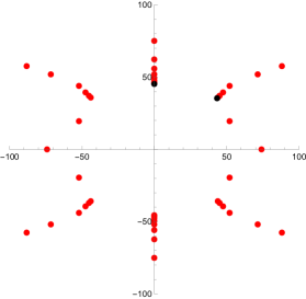
(a) $z=-10^{-6}$

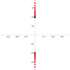
(b) $z=-\frac{9}{270}$

Figure 4.1: Borel singularities of refined Wilson loop BPS sectors $\mathcal{F}[1](\mathsf{b};g_{s})$ for local $\mathbb{P}^{2}$ with $\mathsf{b}=2$ up to $g=50$ in the large radius frame, respectively (a) near the large radius point $z=0$ and (b) near the conifold point $z=-1/27$. The red dots are the approximate singularities from numerical calculations, and the black dots are the indicated branch points, located at (a) $\mathsf{b}^{-1}\mathcal{A}_{(-3,0,0)_{\text{LR}}},\mathsf{b}^{-1}\mathcal{A}_{(-3,1,0)_{\text{LR}}},$ and (b) $\mathsf{b}^{-1}\mathcal{A}_{(-3,0,0)_{\text{LR}}}$ respectively.

(a) $z=-10^{-6}$

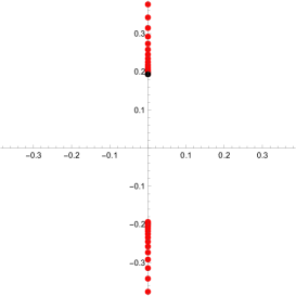
(b) $z=-\frac{9}{270}$

Figure 4.2: Borel singularities of refined Wilson loop BPS sectors $\mathcal{F}[2](\mathsf{b};g_{s})$ for local $\mathbb{P}^{2}$ with $\mathsf{b}=2$ up to $g=50$ in the large radius frame, respectively (a) near the large radius point $z=0$ and (b) near the conifold point $z=-1/27$. The red dots are the approximate singularities from numerical calculations, and the black dots are the indicated branch points, located at (a) $\mathsf{b}^{-1}\mathcal{A}_{(-3,0,0)_{\text{LR}}},\mathsf{b}^{-1}\mathcal{A}_{(-3,1,0)_{\text{LR}}},$ and (b) $\mathsf{b}^{-1}\mathcal{A}_{(-3,0,0)_{\text{LR}}}$ respectively.

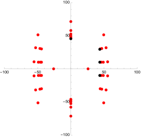
(a) $z=-10^{-6}$

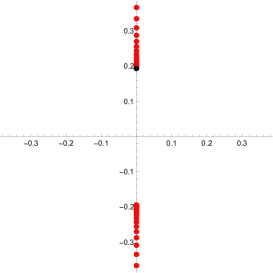
(b) $z=-\frac{9}{270}$

Figure 4.3: Borel singularities of refined free energies $\mathcal{F}[0](\mathsf{b};g_{s})$ for local $\mathbb{P}^{2}$ with $\mathsf{b}=2$ up to $g=50$ in the large radius frame, respectively (a) near the large radius point $z=0$ and (b) near the conifold point $z=-1/27$. The red dots are the approximate singularities from numerical calculations, and the black dots are the indicated branch points, located at (a) $\mathsf{b}^{-1}\mathcal{A}_{(-3,0,0)_{\text{LR}}}$, $\mathsf{b}^{-1}\mathcal{A}_{(0,1,n)_{\text{LR}}}(n=0,1,2)$ and (b) $\mathsf{b}^{-1}\mathcal{A}_{(-3,0,0)_{\text{LR}}}$ respectively.

We first study the location of Borel singularities, i.e. the singular points of the Borel transform. We evaluate the perturbative BPS sectors $\mathcal{F}[1]$ and $\mathcal{F}[2]$ in the holomorphic limit of the large radius frame, where $t_{\mathrm{LR}}$ is the flat coordinate, near respectively the large radius point $z=0$ and the conifold point $z=-1/27$. The Borel singularities of $\mathcal{F}[1]$ and $\mathcal{F}[2]$ are plotted respectively in Figs. 4.1 and Figs. 4.2. The plots are similar for the two BPS sectors. Near the large radius point, the visible Borel singularities are located at $\mathsf{b}^{-1}\mathcal{A}_{\gamma_{\mathrm{LR}}}$ (we take $\mathsf{b}>1$ so that $\mathsf{b}^{-1}\mathcal{A}$ is smaller than $\mathsf{b}\mathcal{A}$) with the charge vectors

$$\gamma_{\mathrm{LR}}=\pm(-3,0,0),\ \pm(-3,\pm 1,0),$$ (4.55)

and we use the notation that

$$\mathcal{A}_{\gamma_{\text{LR}}}=-c{\mathsf{i}}\partial_{t_{\text{LR}}}\mathcal{F}^{(0,0)}_{\text{LR}}+2\pi dt_{\text{LR}}+4\pi^{2}{\mathsf{i}}d_{0},\quad\gamma_{\text{LR}}=(c,d,d_{0}).$$ (4.56)

Near the conifold points, the visible Borel singularities are located at $\mathsf{b}^{-1}\mathcal{A}_{\gamma_{\mathrm{LR}}}$ with

$$\gamma_{\mathrm{LR}}=\pm(-3,0,0).$$ (4.57)

For comparison, we also give the location of Borel singularities for the free energies $\mathcal{F}[0]$ in Figs. 4.3. Near the large radius point, the Borel singularities are located at $\mathsf{b}^{-1}\mathcal{A}_{\gamma_{\mathrm{LR}}}$ with

$$\gamma_{\mathrm{LR}}=\pm(-3,0,0)_{\text{LR}},\;\pm(0,1,n),\,\,n=0,\pm 1,\pm 2,\ldots.$$ (4.58)

Near the conifold point, the Borel singularities are located at $\mathsf{b}^{-1}\mathcal{A}_{\pm(-3,0,0)_{\text{LR}}}$. In contrast to the free energies, the Borel singularities of Wilson loop BPS sectors never coincide with the flat coordinate up to a constant, i.e. the coefficient $c$ in the charge vector $\gamma_{\mathrm{LR}}$ does not vanish.

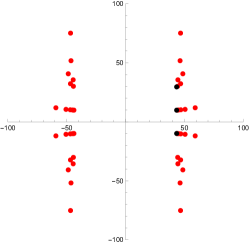
(a) $z=-10^{-6}$

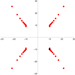
(b) $z=-\frac{9}{270}$

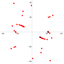
(c) $z=10^{-3}$

Figure 4.4: Borel singularities of refined Wilson loop BPS sectors $\mathcal{F}[1](\mathsf{b};g_{s})$ for local $\mathbb{P}^{2}$ with $\mathsf{b}=2$ up to $g=50$ in the conifold frame, respectively (a) near the large radius point with $z<0$, (c) near the conifold point, and (c) with $z>0$. The red dots are the approximate singularities from numerical calculations, and the black dots are the indicated branch points, located at (a) $\mathsf{b}^{-1}\mathcal{A}_{(-3,0,n)_{\text{c}}}(n=0,1,2)$, (b) $\mathsf{b}^{-1}\mathcal{A}_{(-3,1,0)_{\text{c}}}$ and (c) $\mathsf{b}^{-1}\mathcal{A}_{(-3,0,0)_{\text{c}}}$ (right), $\mathsf{b}^{-1}\mathcal{A}_{(-3,1,0)_{\text{c}}}$ (below) respectively.

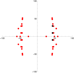
(a) $z=-10^{-6}$

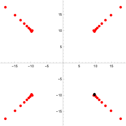
(b) $z=-\frac{9}{270}$

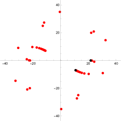
(c) $z=10^{-3}$

Figure 4.5: Borel singularities of refined Wilson loop BPS sectors $\mathcal{F}[2](\mathsf{b};g_{s})$ for local $\mathbb{P}^{2}$ with $\mathsf{b}=2$ up to $g=50$ in the conifold frame, respectively (a) near the large radius point with $z<0$, (b) near the conifold point $z=-1/27$, and (c) with $z>0$. The red dots are the approximate singularities from numerical calculations, and the black dots are the indicated branch points, located at (a) $\mathsf{b}^{-1}\mathcal{A}_{(-3,0,n)_{\text{c}}}(n=0,1,2)$, (c) $\mathsf{b}^{-1}\mathcal{A}_{(-3,1,0)_{\text{c}}}$, and (c) $\mathsf{b}^{-1}\mathcal{A}_{(-3,0,0)_{\text{c}}}$ (right), $\mathsf{b}^{-1}\mathcal{A}_{(-3,1,0)_{\text{c}}}$ (below) respectively.

We also evaluate the perturbative BPS sectors $\mathcal{F}[1]$ and $\mathcal{F}[2]$ in the holomorphic limit of the conifold frame, where $t_{\mathrm{c}}$ is the flat coordinate. Similarly, we focus on the loci near respectively the large radius point $z=0$ and the conifold point $z=-1/27$. The Borel singularities are shown in Figs. 4.4 and Figs. 4.5 respectively. In both examples, we find that near the large radius point with $z<0$ (we take $\mathsf{b}>1$ so that $\mathsf{b}^{-1}\mathcal{A}$ is smaller than $\mathsf{b}\mathcal{A}$), the visible Borel singularities are as usual located at $\mathsf{b}^{-1}\mathcal{A}_{\gamma_{\mathrm{c}}}$ with charge vectors

$$\gamma_{\text{c}}=\pm(-3,0,\pm n),\quad n=1,2,3....$$ (4.59)

Near the conifold point, the visible Borel singularities are located at $\mathsf{b}^{-1}\mathcal{A}_{\pm(-3,\pm 1,0)}$. Here we denote by $\mathcal{A}_{\gamma_{\text{c}}}$

$$\mathcal{A}_{\gamma_{\text{c}}}=-c^{\prime}{\mathsf{i}}\partial_{t_{\text{c}}}\mathcal{F}^{(0,0)}_{\text{c}}+2\pi d^{\prime}t_{\text{c}}+4\pi^{2}{\mathsf{i}}d^{\prime}_{0},\quad\gamma_{\text{c}}=(c^{\prime},d^{\prime},d^{\prime}_{0}),$$ (4.60)

and the two charge conventions $\gamma_{\text{LR}}$ and $\gamma_{\text{c}}$ are related to each other via the relationship

$$\gamma_{\text{c}}=\begin{pmatrix}0&-3&0\\ \frac{1}{3}&0&0\\ 0&0&1\end{pmatrix}\gamma_{\text{LR}},\quad\gamma_{\text{LR}}=\begin{pmatrix}0&3&0\\ -\frac{1}{3}&0&0\\ 0&0&1\end{pmatrix}\gamma_{\text{c}}.$$ (4.61)

In addition, we also consider the loci at $z>0$, and we find visible Borel singularities

$$\gamma_{\text{c}}=\pm(-3,1,0),\;\pm(-3,0,0),$$ (4.62)

as shown in Figs. 4.4 (c), 4.5 (c). We find yet again that none of the Borel singularities coincide with the flat coordinate up to a constant, i.e. the coefficient $c^{\prime}$ in $\gamma_{\text{c}}$ does not vanish.

Next, we study the non-perturbative series. We focus on the 1-instanton sector, and check the coefficients of the non-perturbative series (4.10) in the generic refined case, and (4.22) in the unrefined limit with $\mathsf{b}=1$. In the generic refined case, the 1-instanton non-perturbative series can be written as

$$\mathcal{F}^{(1)}[m]=g_{s}^{m}{\rm e}^{-\tilde{\mathcal{A}}/g_{s}}(\mu_{0}+\mu_{1}g_{s}+\mu_{2}g_{s}^{2}+\ldots)$$ (4.63)

with $\tilde{A}$ being either $\mathsf{b}^{-1}\mathcal{A}$ or $\mathsf{b}\mathcal{A}$. Compared with the form of perturbative series (4.2), standard resurgence analysis predicts the large order asymptotics of the perturbative coefficients

$$\mathcal{F}_{g}[m]\sim\frac{\mathsf{S}}{\pi{\mathsf{i}}}\frac{\Gamma(2g+m-2)}{\tilde{\mathcal{A}}^{2g+m-2}}\left(\mu_{0}+\frac{\mu_{1}\tilde{\mathcal{A}}}{2g+m-3}+\frac{\mu_{2}\tilde{\mathcal{A}}}{(2g+m-3)(2g+m-4)}+\ldots\right).$$ (4.64)

where $\tilde{\mathcal{A}}$ is the dominant Borel singularity, the closest to the origin, and we have taken into account that both $\pm\tilde{\mathcal{A}}$ sectors contribute equally to the asymptotic formula. In the unrefined limit with $\mathsf{b}=1$, the 1-instanton non-perturbative series can be written as

$$\mathcal{F}^{(1)}[m]=g_{s}^{m-1}{\rm e}^{-\tilde{\mathcal{A}}/g_{s}}(\mu_{0}+\mu_{1}g_{s}+\mu_{2}g_{s}^{2}+\ldots)$$ (4.65)

and the large order asymptotics should be modified to

$$\mathcal{F}_{g}[m]\sim\frac{\mathsf{S}}{\pi{\mathsf{i}}}\frac{\Gamma(2g+m-1)}{\tilde{\mathcal{A}}^{2g+m-1}}\left(\mu_{0}+\frac{\mu_{1}\tilde{\mathcal{A}}}{2g+m-2}+\frac{\mu_{2}\tilde{\mathcal{A}}}{(2g+m-2)(2g+m-3)}+\ldots\right).$$ (4.66)

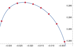
(a) $\mu_{0}$

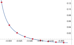
(b) $\mu_{1}$

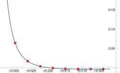
(c) $\mu_{2}$

Figure 4.6: Comparison for local $\mathbb{P}^{2}$ between numerical results (red dots) of $\frac{1}{\pi{\mathsf{i}}}\mathsf{S}\cdot\mu_{0,1,2}$ extracted from the large order asymptotics of $\mathcal{F}_{g}[1]$ up to $g=50$ in the large radius frame at $\mathsf{b}=2$ with error bars (vertical bars, virtually invisible) and trans-series solutions from HAE (solid line). Richardson transformation of degree 10 is used to improve the numerics. The horizontal axis is modulus $z$.

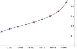
(a) $\mu_{0}$

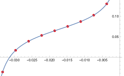
(b) $\mu_{1}$

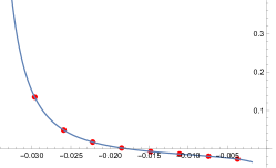
(c) $\mu_{2}$

Figure 4.7: Comparison for local $\mathbb{P}^{2}$ for local $\mathbb{P}^{2}$ between numerical results (red dots) of $\frac{1}{\pi{\mathsf{i}}}\mathsf{S}\cdot\mu_{0,1,2}$ extracted from the large order asymptotics of $\mathcal{F}_{g}[2]$ up to $g=50$ in the large radius frame at $\mathsf{b}=2$ with error bars (vertical bars, virtually invisible) and trans-series solutions from HAE (solid line). Richardson transformation of degree 10 is used to improve the numerics. The horizontal axis is modulus $z$.

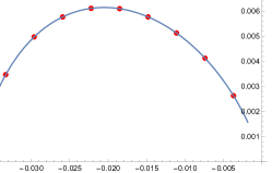
(a) $\mu_{0}$

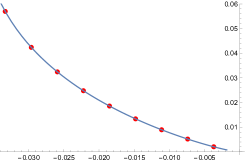
(b) $\mu_{1}$

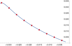
(c) $\mu_{2}$

Figure 4.8: Comparison for local $\mathbb{P}^{2}$ between numerical results (red dots) of $\frac{1}{\pi{\mathsf{i}}}\mathsf{S}\cdot\mu_{0,1,2}$ extracted from the large order asymptotics of $\mathcal{F}_{g}[1]$ up to $g=100$ in the large radius frame at $\mathsf{b}=1$ with error bars (vertical bars, virtually invisible) and trans-series solutions from HAE (solid line). Richardson transformation of degree 15 is used to improve the numerics. The horizontal axis is modulus $z$.

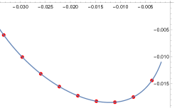
(a) $\mu_{0}$

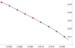
(b) $\mu_{1}$

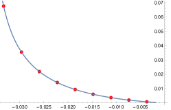
(c) $\mu_{2}$

Figure 4.9: Comparison for local $\mathbb{P}^{2}$ between numerical results (red dots) of $\frac{1}{\pi{\mathsf{i}}}\mathsf{S}\cdot\mu_{0,1,2}$ extracted from the large order asymptotics of $\mathcal{F}_{g}[2]$ up to $g=100$ in the large radius frame at $\mathsf{b}=1$ with error bars (vertical bars, virtually invisible) and trans-series solutions from HAE (solid line). Richardson transformation of degree 15 is used to improve the numerics. The horizontal axis is modulus $z$.

We consider two different cases. The first is the BPS sectors near the conifold point in the large radius frame. The dominant Borel singularities are the pair of $\gamma_{\text{LR}}=\pm(-3,0,0)$ as shown in Figs. 4.1 (b), 4.2 (b). The large order asymptotics formula (4.64) (formula (4.66) in the unrefined limit) can be used to extract the non-perturbative coefficients $\mu_{0},\mu_{1},\mu_{2},\ldots$, and we compare these numerical results with our prediction from Sections 4.1 and 4.2.1 in Figs. 4.6, 4.7 for generic $\mathsf{b}$, and in Fig. 4.23 in the unrefined limit. The numerical results and the theoretical predictions match perfectly, as long as we choose the Stokes constants

$$\mathsf{S}_{\pm(-3,0,0)_{\text{LR}}}(\mathsf{b})=1,$$ (4.67)

corresponding to the spin 0 BPS state of D4 brane wrapping $\mathbb{P}^{2}$ in type IIA superstring.

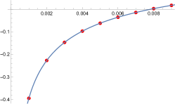
(a) $\mu_{0}$

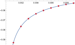
(b) $\mu_{1}$

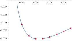
(c) $\mu_{2}$

Figure 4.10: Comparison for local $\mathbb{P}^{2}$ in the conifold frame at $\mathsf{b}=2$ with large positive $z$ between numerical results (red dots) of $\frac{1}{\pi{\mathsf{i}}}\mathsf{S}\cdot\mu_{0,1,2}$ for $\mathcal{A}_{\pm(-3,1,0)_{\text{c}}}$ extracted from the large order asymptotics of $\mathcal{F}_{g}[1]$ up to $g=50$ with error bars (vertical bars, virtually invisible) and trans-series solutions from HAE (solid line). Richardson transformation of degree 5 is used to improve the numerics. The horizontal axis is modulus $z$.

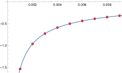
(a) $\mu_{0}$

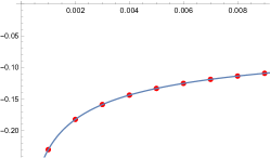
(b) $\mu_{1}$

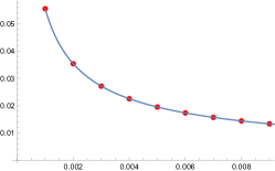
(c) $\mu_{2}$

Figure 4.11: Comparison for local $\mathbb{P}^{2}$ in the conifold frame at $\mathsf{b}=2$ with large positive $z$ between numerical results (red dots) of $\frac{1}{\pi{\mathsf{i}}}\mathsf{S}\cdot\mu_{0,1,2}$ for $\mathcal{A}_{\pm(-3,1,0)_{\text{c}}}$ extracted from the large order asymptotics of $\mathcal{F}_{g}[2]$ up to $g=50$ with error bars (vertical bars, virtually invisible) and trans-series solutions from HAE (solid line). Richardson transformation of degree 5 is used to improve the numerics. The horizontal axis is modulus $z$.

Similarly, we consider the BPS sectors at $z>0$ in the conifold frame. Depending on the actual value of $z$, the two pairs of Borel singularities $\gamma_{\text{c}}=\pm(-3,1,0)$ and $\gamma_{\text{c}}=\pm(-3,0,0)$ compete in dominance, as shown in Fig. 4.4 (c), 4.5 (c). If $z\gtrsim 4\times 10^{-6}$, the pair of $\gamma_{\text{c}}=\pm(-3,1,0)_{\text{c}}$ is dominant (closer to the origin). The comparison between the numerical results of $\mu_{0},\mu_{1},\mu_{2}$ from large order asymptotics and theoretical predictions are plotted in Figs. 4.10, 4.11. Here we have chosen the Stokes constants

$$\mathsf{S}_{\pm(-3,1,0)_{\text{c}}}(\mathsf{b})=\mathsf{S}_{\pm(3,1,0)_{\text{LR}}}(\mathsf{b})=1,$$ (4.68)

where we have used the charge vector relations (4.61), and they correspond to the spin 0 BPS states of D4 brane wrapping $\mathbb{P}^{2}$ together with a D2 brane wrapping $\mathbb{P}^{1}\subset\mathbb{P}^{2}$.

(a) $\mu_{0}$

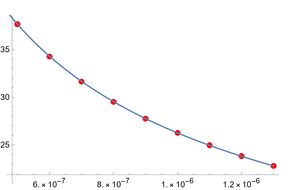
(b) $\mu_{1}$

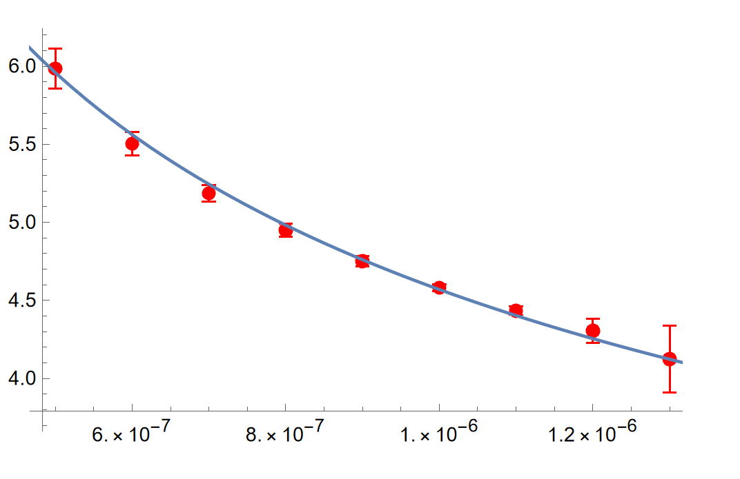
(c) $\mu_{2}$

Figure 4.12: Comparison for local $\mathbb{P}^{2}$ in the conifold frame at $\mathsf{b}=1$ with small and positive $z$ between numerical results (red dots) of $\frac{1}{\pi{\mathsf{i}}}\mathsf{S}\cdot\mu_{0,1,2}$ for $\mathcal{A}_{\pm(-3,0,0)_{\text{c}}}$ extracted from the large order asymptotics of $\mathcal{F}_{g}[1]$ up to $g=100$ with error bars (vertical bars, virtually invisible) and trans-series solutions from HAE (solid line). Richardson transformation of degree 5 is used to improve the numerics. The horizontal axis is modulus $z$.

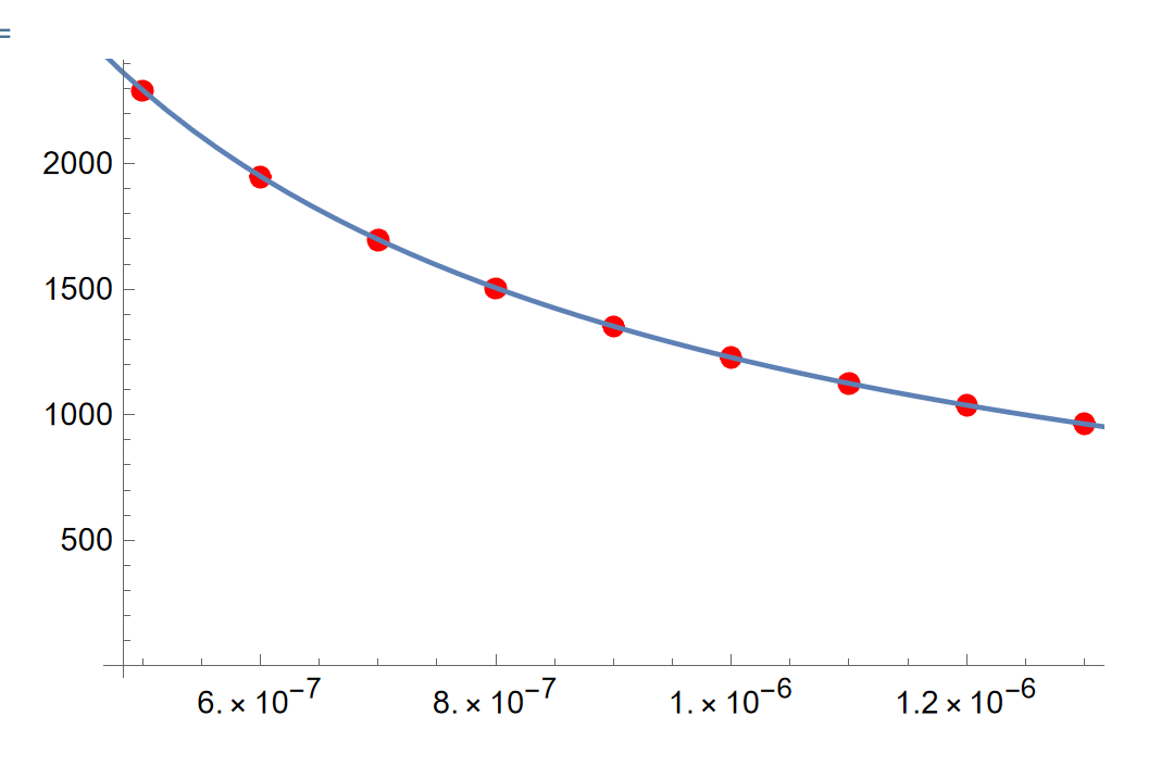
(a) $\mu_{0}$

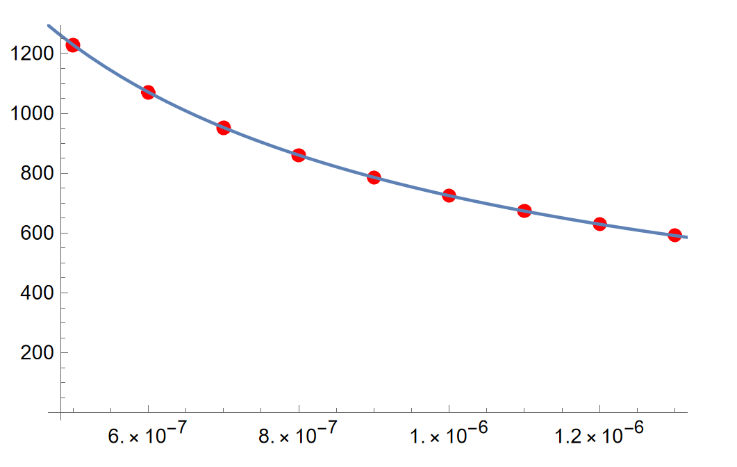
(b) $\mu_{1}$

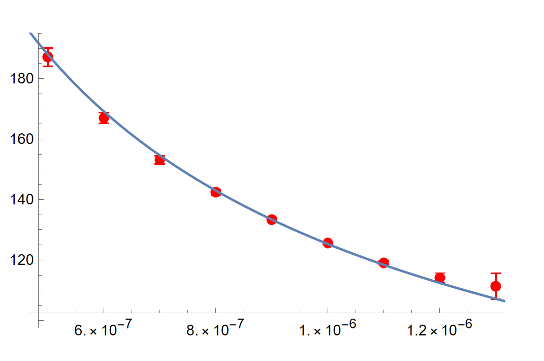
(c) $\mu_{2}$

Figure 4.13: Comparison for local $\mathbb{P}^{2}$ in the conifold frame at $\mathsf{b}=1$ with small and positive $z$ between numerical results (red dots) of $\frac{1}{\pi{\mathsf{i}}}\mathsf{S}\cdot\mu_{0,1,2}$ for $\mathcal{A}_{\pm(-3,0,0)_{\text{c}}}$ extracted from the large order asymptotics of $\mathcal{F}_{g}[2]$ up to $g=100$ with error bars (vertical bars, virtually invisible) and trans-series solutions from HAE (solid line). Richardson transformation of degree 5 is used to improve the numerics. The horizontal axis is modulus $z$.

Finally, if $0<z\lesssim 4\times 10^{-6}$, the pair of $\gamma_{\text{c}}=\pm(-3,0,0)_{\text{c}}$ is dominant, and the plots for $\mu_{0},\mu_{1},\mu_{2}$ are given in Figs. 4.12, 4.13. Here we have chosen the Stokes constants

$$\mathsf{S}_{\pm(-3,0,0)_{\text{c}}}(\mathsf{b})=\mathsf{S}_{\pm(0,1,0)_{\text{LR}}}(\mathsf{b})=3\chi_{1/2}(-{\rm e}^{-\pi{\mathsf{i}}/\mathsf{b}^{2}}),$$ (4.69)

corresponding to the well-known spin 1/2 BPS states of a single D2 brane wrapping $\mathbb{P}^{1}\subset\mathbb{P}^{2}$.

4.4 Example: local $\mathbb{P}^{1}\times\mathbb{P}^{1}$

Similar to Section 4.3, we consider the example of refined topological string theory on local $\mathbb{P}^{1}\times\mathbb{P}^{1}$, i.e. the total space of the canonical bundle of $\mathbb{P}^{1}\times\mathbb{P}^{1}$, with the constraint that the two $\mathbb{P}^{1}$s have the same volume, also known as the massless limit. This theory has also been discussed in detail in the literature. It has a one dimensional moduli space with three singular points of large radius, conifold, and orbifold types Haghighat:2008gw , and we take the convention that it is parametrised by the global complex coordinate $z$, such that the three singular points are located at $z=0$, $z=1/16$, and $z=\infty$ respectively.

The periods of the theory are annihilated by the Picard-Fuchs operator Chiang:1999tz

$$\mathcal{L}=(1-16z)\partial_{z}+z(3-64z)\partial_{z}^{2}+z^{2}(1-16z)\partial_{z}^{3}.$$ (4.70)

Near the large radious point, the flat coordinate and its conjugate are (see e.g. Marino:2015ixa )

$$t_{\text{LR}}= -\log(z)-4z{}_{4}F_{3}(1,1,\tfrac{3}{2},\tfrac{3}{2};2,2,2;16z),$$

$$\frac{\partial\mathcal{F}^{(0,0)}_{\text{LR}}}{\partial t_{\text{LR}}}= \frac{1}{\pi}G^{3,2}_{3,3}\left(\begin{array}[]{c}\tfrac{1}{2},\tfrac{1}{2};1\\ 0,0,0\end{array};16z\right)-\pi^{2},$$ (4.71c)

while near the conifold point, the flat coordinate and its conjugate are

$$t_{\text{c}}= \frac{1}{\pi{\mathsf{i}}}\frac{\partial\mathcal{F}^{(0,0)}_{\text{LR}}}{\partial t_{\text{LR}}},$$

$$\frac{\partial\mathcal{F}^{(0,0)}_{\text{c}}}{\partial t_{\text{c}}}= -\pi{\mathsf{i}}t_{\text{LR}}.$$ (4.72a)

As in Section 4.3, we first inspect the non-perturbative corrections for Wilson loop BPS sectors, which can be calculated effectively using the algorithm in Wang:2023zcb . For simplicity, we focus on the range between the large radious point $z=0$ and the conifold point $z=1/16$.

(a) $z=10^{-6}$

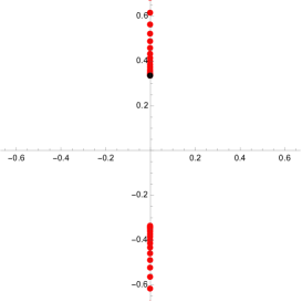
(b) $z=\frac{9}{160}$

Figure 4.14: Borel singularities of refined Wilson loop BPS sectors $\mathcal{F}[1](\mathsf{b};g_{s})$ for local $\mathbb{P}^{1}\times\mathbb{P}^{1}$ with $\mathsf{b}=2$ up to $g=50$ in the large radius frame, respectively (a) near the large radius point $z=0$ and (b) near the conifold point $z=1/16$. The red dots are the approximate singularities from numerical calculations, and the black dots are the indicated branch points, located at (a) $\mathsf{b}^{-1}\mathcal{A}_{(-2,0,0)_{\text{LR}}},\mathsf{b}^{-1}\mathcal{A}_{(-2,1,0)_{\text{LR}}},\mathsf{b}^{-1}\mathcal{A}_{(-2,2,-1)_{\text{LR}}},\mathsf{b}^{-1}\mathcal{A}_{(-2,3,-2)_{\text{LR}}}$ and (b) $\mathsf{b}^{-1}\mathcal{A}_{(-2,0,0)_{\text{LR}}}$ respectively.

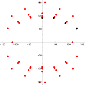
(a) $z=10^{-6}$

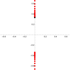
(b) $z=\frac{9}{160}$

Figure 4.15: Borel singularities of refined Wilson loop BPS sectors $\mathcal{F}[2](\mathsf{b};g_{s})$ for local $\mathbb{P}^{1}\times\mathbb{P}^{1}$ with $\mathsf{b}=2$ up to $g=50$ in the large radius frame, respectively (a) near the large radius point $z=0$ and (b) near the conifold point $z=1/16$. The red dots are the approximate singularities from numerical calculations, and the black dots are the indicated branch points, located at (a) $\mathsf{b}^{-1}\mathcal{A}_{(-2,0,0)_{\text{LR}}},\mathsf{b}^{-1}\mathcal{A}_{(-2,1,0)_{\text{LR}}},\mathsf{b}^{-1}\mathcal{A}_{(-2,2,-1)_{\text{LR}}},\mathsf{b}^{-1}\mathcal{A}_{(-2,3,-2)_{\text{LR}}}$ and (b) $\mathsf{b}^{-1}\mathcal{A}_{(-2,0,0)_{\text{LR}}}$ respectively.

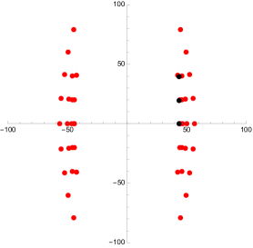
(a) $z=10^{-6}$

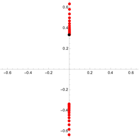
(b) $z=\frac{9}{160}$

Figure 4.16: Borel singularities of refined free energies $\mathcal{F}[0](\mathsf{b};g_{s})$ for local $\mathbb{P}^{1}\times\mathbb{P}^{1}$ with $\mathsf{b}=2$ up to $g=50$ in the large radius frame, respectively (a) near the large radius point $z=0$ and (b) near the conifold point $z=1/16$. The red dots are the approximate singularities from numerical calculations, and the black dots are the indicated branch points, located at (a) $\mathsf{b}^{-1}\mathcal{A}_{(0,1,n)_{\text{LR}}}$ ($n=0,1,2$) and (b) $\mathsf{b}^{-1}\mathcal{A}_{(-2,0,0)_{\text{LR}}}$ respectively.

Let us study the location of Borel singularities first. We evaluate the perturbative BPS sectors $\mathcal{F}[1]$ and $\mathcal{F}[2]$ in the holomorphic limit of the large radius frame, where $t_{\text{LR}}$ is the flat coordinate, near respectively the large radius point $z=0$ and the conifold point $z=1/16$. The Borel singularities of $\mathcal{F}[1]$ and $\mathcal{F}[2]$ are plotted in Figs. 4.14 and Figs. 4.15. These two plots are similar. Near the large radius point, the visible Borel singularities are located at $\mathsf{b}^{-1}\mathcal{A}_{\gamma_{\text{LR}}}$ (we take $\mathsf{b}>1$ so that $\mathsf{b}^{-1}\mathcal{A}$ is smaller than $\mathsf{b}\mathcal{A}$) with the charges

$$\gamma_{\text{LR}}=\pm(-2,0,0),\pm(-2,\pm(1+n),-n),\;\;n=0,1,2,\ldots.$$ (4.73)

Near the conifold point, the visible Borel singularities are located at $\mathsf{b}^{-1}\mathcal{A}_{\pm(-2,0,0)_{\text{LR}}}$. For comparison, we also give the same plots for the free energies $\mathcal{F}[0]$ in Figs. 4.16. The visible Borel singularities are located at $\mathsf{b}^{-1}\mathcal{A}_{\gamma_{\text{LR}}}$ with

$$\gamma_{\text{LR}}=\pm(0,1,n),\;\;n=0,\pm 1,\pm 2,\ldots,$$ (4.74)

near the large radius point and at $\mathsf{b}^{-1}\mathcal{A}_{\pm(-2,0,0)_{\text{LR}}}$ near the conifold point. The same as local $\mathbb{P}^{2}$, the Borel singularities of Wilson loop BPS sectors never coincide with the flat coordinate up to a constant, i.e. the first coefficient in the charge vector $\gamma_{\text{LR}}$ does not vanish.

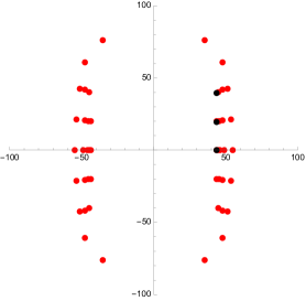
(a) $z=10^{-6}$

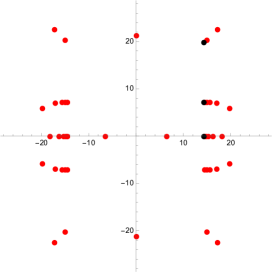
(b) $z=10^{-2}$

Figure 4.17: Borel singularities of refined Wilson loop BPS sectors $\mathcal{F}[1](\mathsf{b};g_{s})$ for local $\mathbb{P}^{1}\times\mathbb{P}^{1}$ with $\mathsf{b}=2$ up to $g=50$ in the conifold frame, respectively (a) very close to the large radius point and (b) away from it toward the conifold point. The red dots are the approximate singularities from numerical calculations, and the black dots are the indicated branch points, located at (a) $\mathsf{b}^{-1}\mathcal{A}_{(0,1,n)_{\text{LR}}}$ ($n=0,1,2$) and (b) $\mathsf{b}^{-1}\mathcal{A}_{(-2,0,0)_{\text{c}}},\mathsf{b}^{-1}\mathcal{A}_{(-2,1,0)_{\text{c}}},\mathsf{b}^{-1}\mathcal{A}_{(-2,0,1)_{\text{c}}}$ respectively.

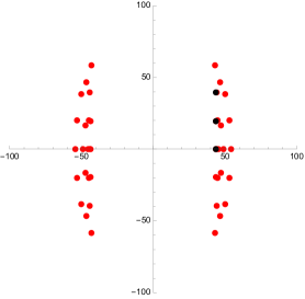
(a) $z=10^{-6}$

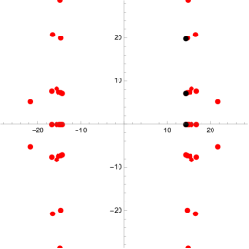
(b) $z=10^{-2}$

Figure 4.18: Borel singularities of refined Wilson loop BPS sectors $\mathcal{F}[2](\mathsf{b};g_{s})$ for local $\mathbb{P}^{1}\times\mathbb{P}^{1}$ with $\mathsf{b}=2$ up to $g=50$ in the conifold frame, respectively (a) very close to the large radius point and (b) away from it toward the conifold point. The red dots are the approximate singularities from numerical calculations, and the black dots are the indicated branch points, located at (a) $\mathsf{b}^{-1}\mathcal{A}_{(0,1,n)_{\text{LR}}}$ ($n=0,1,2$) and (b) $\mathsf{b}^{-1}\mathcal{A}_{(-2,0,0)_{\text{c}}},\mathsf{b}^{-1}\mathcal{A}_{(-2,1,0)_{\text{c}}},\mathsf{b}^{-1}\mathcal{A}_{(-2,0,1)_{\text{c}}}$ respectively.

We also evaluate the perturbative BPS sectors $\mathcal{F}[1]$ and $\mathcal{F}[2]$ in the holomorphic limit of the conifold frame, where $t_{\text{c}}$ is the flat coordinate, respectively very close to the large radius point, and away from it toward the conifold point. The Borel singularities are plotted respectively in Figs. 4.17 and Figs. 4.18. In both examples, the visible Borel singularities are located at $\mathsf{b}^{-1}\mathcal{A}_{\gamma_{\text{c}}}$ with

$$\gamma_{\text{c}}=\pm(-2,0,n),\;\;n=0,\pm 1,\pm 2,\ldots,$$ (4.75)

near the large radius point, and at $\mathsf{b}^{-1}\mathcal{A}_{\text{c}}$ with

$$\gamma_{\text{c}}=\pm(-2,0,0),\;\pm(-2,\mp 1,0),\pm(-2,0,\pm 1),$$ (4.76)

near the conifold point (we take $\mathsf{b}>1$ so that $\mathsf{b}^{-1}\mathcal{A}$ is smaller than $\mathsf{b}\mathcal{A}$). Similarly, none of the Borel singularities coincide with the flat coordinate up to a constant, i.e. the first coefficient in the charge vector $\gamma_{\text{c}}$ does not vanish. Note that we have used two types of charge vectors $\gamma_{\text{LR}}$ and $\gamma_{\text{c}}$ defined respectively in (4.56) and (4.60) , which are related to each other in the case of local $\mathbb{P}^{1}\times\mathbb{P}^{1}$ by

$$\gamma_{\text{c}}=\begin{pmatrix}0&-2&0\\ \frac{1}{2}&0&0\\ 0&0&1\end{pmatrix}\gamma_{\text{LR}},\quad\gamma_{\text{LR}}=\begin{pmatrix}0&2&0\\ -\frac{1}{2}&0&0\\ 0&0&1\end{pmatrix}\gamma_{\text{c}}.$$ (4.77)

Next, we study the non-perturbative series. We focus on the 1-instanton sector as Section in 4.4. The large order asymptotics of the perturbative coefficients are the same as (4.64) and (4.66). We consider two cases, the BPS sectors near the conifold point in the large radius frame, as well as in the conifold frame. The dominant Borel singularities are respectively $\gamma_{\text{LR}}=\pm(-2,0,0)$ and $\gamma_{\text{c}}=\pm(-2,0,0)$, as shown in the plots of Figs. 4.14 (b), 4.15 (b) and Figs. 4.17 (b), 4.18 (b). we compare these numerical results of $\mu_{0},\mu_{1},\mu_{2},\ldots$ extracted from perturbative data using the large order formulas with the theoretical prediction from Sections 4.1 and 4.2.1 in Figs. 4.19, 4.20, 4.21, 4.22 for generic $\mathsf{b}$, and in Figs. 4.23, 4.24, 4.25, 4.26 for the unrefined limit $\mathsf{b}=1$.

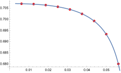
(a) $\mu_{0}$

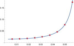
(b) $\mu_{1}$

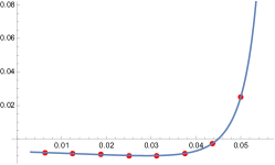
(c) $\mu_{2}$

Figure 4.19: Comparison for local $\mathbb{P}^{1}\times\mathbb{P}^{1}$ between numerical results (red dots) of $\frac{1}{\pi{\mathsf{i}}}\mathsf{S}\cdot\mu_{0,1,2}$ extracted from the large order asymptotics of $\mathcal{F}_{g}[1]$ up to $g=50$ in the large radius frame at $\mathsf{b}=2$ with error bars (vertical bars, virtually invisible) and trans-series solutions from HAE (solid line). Richardson transformation of degree 10 is used to improve the numerics. The horizontal axis is modulus $z$.

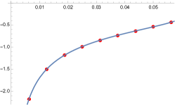
(a) $\mu_{0}$

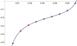
(b) $\mu_{1}$

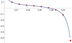
(c) $\mu_{2}$

Figure 4.20: Comparison for local $\mathbb{P}^{1}\times\mathbb{P}^{1}$ between numerical results (red dots) of $\frac{1}{\pi{\mathsf{i}}}\mathsf{S}\cdot\mu_{0,1,2}$ extracted from the large order asymptotics of $\mathcal{F}_{g}[2]$ up to $g=50$ in the large radius frame at $\mathsf{b}=2$ with error bars (vertical bars, virtually invisible) and trans-series solutions from HAE (solid line). Richardson transformation of degree 10 is used to improve the numerics. The horizontal axis is modulus $z$.

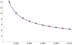
(a) $\mu_{0}$

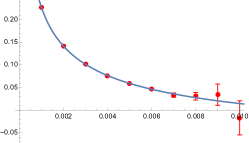
(b) $\mu_{1}$

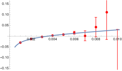
(c) $\mu_{2}$

Figure 4.21: Comparison for local $\mathbb{P}^{1}\times\mathbb{P}^{1}$ between numerical results (red dots) of $\frac{1}{\pi{\mathsf{i}}}\mathsf{S}\cdot\mu_{0,1,2}$ extracted from the large order asymptotics of $\mathcal{F}_{g}[1]$ up to $g=50$ in conifold frame at $\mathsf{b}=2$ with error bars (vertical bars) and trans-series solutions from HAE (solid line). Richardson transformation of degree 10 is used to improve the numerics. The horizontal axis is modulus $z$.

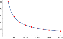
(a) $\mu_{0}$

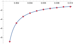
(b) $\mu_{1}$

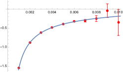
(c) $\mu_{2}$

Figure 4.22: Comparison for local $\mathbb{P}^{1}\times\mathbb{P}^{1}$ between numerical results (red dots) of $\frac{1}{\pi{\mathsf{i}}}\mathsf{S}\cdot\mu_{0,1,2}$ extracted from the large order asymptotics of $\mathcal{F}_{g}[2]$ up to $g=50$ in conifold frame at $\mathsf{b}=2$ with error bars (vertical bars) and trans-series solutions from HAE (solid line). Richardson transformation of degree 10 is used to improve the numerics. The horizontal axis is modulus $z$.

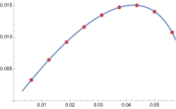
(a) $\mu_{0}$

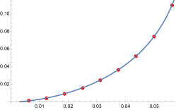
(b) $\mu_{1}$

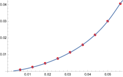
(c) $\mu_{2}$

Figure 4.23: Comparison for local $\mathbb{P}^{1}\times\mathbb{P}^{1}$ between numerical results (red dots) of $\frac{1}{\pi{\mathsf{i}}}\mathsf{S}\cdot\mu_{0,1,2}$ extracted from the large order asymptotics of $\mathcal{F}_{g}[1]$ up to $g=100$ in the large radius frame at $\mathsf{b}=1$ with error bars (vertical bars, virtually invisible) and trans-series solutions from HAE (solid line). Richardson transformation of degree 10 is used to improve the numerics. The horizontal axis is modulus $z$.

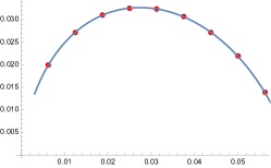
(a) $\mu_{0}$

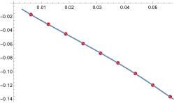
(b) $\mu_{1}$

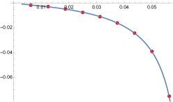
(c) $\mu_{2}$

Figure 4.24: Comparison for local $\mathbb{P}^{1}\times\mathbb{P}^{1}$ between numerical results (red dots) of $\frac{1}{\pi{\mathsf{i}}}\mathsf{S}\cdot\mu_{0,1,2}$ extracted from the large order asymptotics of $\mathcal{F}_{g}[2]$ up to $g=100$ in the large radius frame at $\mathsf{b}=1$ with error bars (vertical bars, virtually invisible) and trans-series solutions from HAE (solid line). Richardson transformation of degree 10 is used to improve the numerics. The horizontal axis is modulus $z$.

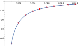
(a) $\mu_{0}$

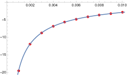
(b) $\mu_{1}$

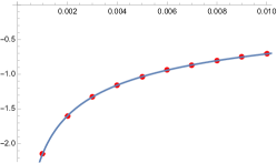
(c) $\mu_{2}$

Figure 4.25: Comparison for local $\mathbb{P}^{1}\times\mathbb{P}^{1}$ between numerical results (red dots) of $\frac{1}{\pi{\mathsf{i}}}\mathsf{S}\cdot\mu_{0,1,2}$ extracted from the large order asymptotics of $\mathcal{F}_{g}[1]$ up to $g=100$ in the conifold frame at $\mathsf{b}=1$ with error bars (vertical bars, virtually invisible) and trans-series solutions from HAE (solid line). Richardson transformation of degree 10 is used to improve the numerics. The horizontal axis is modulus $z$.

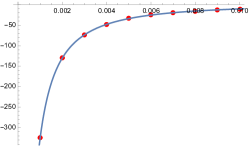
(a) $\mu_{0}$

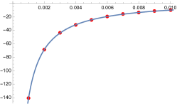
(b) $\mu_{1}$

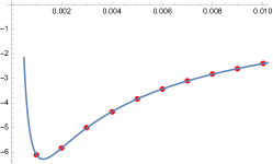
(c) $\mu_{2}$

Figure 4.26: Comparison for local $\mathbb{P}^{1}\times\mathbb{P}^{1}$ between numerical results (red dots) of $\frac{1}{\pi{\mathsf{i}}}\mathsf{S}\cdot\mu_{0,1,2}$ extracted from the large order asymptotics of $\mathcal{F}_{g}[2]$ up to $g=100$ in the conifold frame at $\mathsf{b}=1$ with error bars (vertical bars, virtually invisible) and trans-series solutions from HAE (solid line). Richardson transformation of degree 10 is used to improve the numerics. The horizontal axis is modulus $z$.

Finally, we note that the numerical results and the theoertical prediction can match very well, as shown in the above Figures, only if we have taken the Stokes constant associated to $\mathcal{A}_{\pm(-2,0,0)_{\text{LR}}}$ to be

$$\mathsf{S}_{\pm(-2,0,0)_{\text{LR}}}(\mathsf{b})=1,$$ (4.78)

and the Stokes constant associated to $\mathcal{A}_{\pm(-2,0,0)_{\text{c}}}$ to be

$$\mathsf{S}_{\pm(-2,0,0)_{\text{c}}}(\mathsf{b})=2\chi_{1/2}(-{\rm e}^{-\pi{\mathsf{i}}/\mathsf{b}^{2}}).$$ (4.79)

The Borel singularities $\mathcal{A}_{\pm\gamma_{1}}$ with $\gamma_{1}=(2,0,0)_{\text{LR}}$ are associated to the spin 0 BPS state of D4 brane wrapping $\mathbb{P}^{1}\times\mathbb{P}^{1}$ in type II superstring, and the refined DT-invariant is

$$\Omega(\gamma_{1},y)=1.$$ (4.80)

The Borel singularities $\mathcal{A}_{\pm\gamma_{2}}$ with $\gamma_{2}=(-2,0,0)_{\text{c}}=(0,1,0)_{\text{LR}}$ are associated to the spin $1/2$ BPS state of D2 brane wrapping either $\mathbb{P}^{1}$ in type IIA superstring, and the refined DT-invarint is

$$\Omega(\gamma_{2},y)=2\chi_{1/2}(y).$$ (4.81)

Therefore the Stokes constants agree with the refined DT-invariants, in accord with our prediction from Section 4.1.

5 Conclusion

In this paper, we study the resurgent structures of refined Wilson loops in topological string theory on a local Calabi-Yau threefold. The refined Wilson loops are treated as asymptotic series in $g_{s}$ with deformation parameter $\mathsf{b}$, using the parametrisation (2.16). We find that they are very similar to those of refined free energies. The non-perturbative actions are integral periods, but they cannot be local flat coordinates or equivalent A-periods in the B-model. The non-perturbative trans-series can be solved in closed form from the holomorphic anomaly equations for Wilson loops, and finally, the Stokes constants are identified with refined DT invariants.

There are many interesting open problems related to this work. First of all, Wilson loop is a concept borrowed from 5d $\mathcal{N}=1$ gauge theory, related to topological string via geometric engineering Katz:1996fh . Here we consider Wilson loops in 5d gauge theories, which are codimension four defects. Defects of other codimensions and of other natures exist. One other important type of defects in 5d gauge theories is codimension two defects, and their partition functions play the role of wave-functions in quantum mirror curve. It is argued in Grassi:2022zuk with the simple example of topological string on $\mathbb{C}^{3}$ or the resolved conifold that the Borel singularities of these wave-functions should correspond to BPS states of 3d/5d coupled systems. Similarly it was found that the Borel singularities of wave-functions of quantum Seiberg-Witten curves of 4d $\mathcal{N}=2$ gauge theories correspond to BPS states of 2d/4d coupled systems. It would be interesting to generalise these results to the generic setup in topological string, and to also find out the non-perturbative series associated to these BPS states of the coupled systems.

Second, there has been now convincing evidence that the Stokes constants of both the refined free energies and the refined Wilson loops are the refined DT invariants. It would be certainly nice to work out a rigorous proof. Another interesting direction is to use Stokes constants to help with the calculation of DT invariants, or to study the stability walls. In this regard, Wilson loops can sometimes yield more information than free energies, as shown by the Borel singularities of charge vectors (4.73), which should correspond to non-trivial BPS states for local $\mathbb{P}^{1}\times\mathbb{P}^{1}$. The explicit calculation of Stokes constants associated to these singularities, and beyond, is numerically challenging, but the results in Gu:2021ize in the special conifold limit could be a promising start.

Third, the evaluation of either the refined free energy or the refined Wilson loops depends on a choice of frame. It has been observed in Gu:2022sqc ; Gu:2023mgf and also in this paper that the calculation of Stokes constants is independent of this choice. This is natural as the DT invariants, which are conjectured to identify with the Stokes constants, know nothing of the frame. It would nevertheless be reassuring if one can find a proof of this observation.

Finally, the DT invariants which are conjectured to coincide with Stokes constants are counting of stable bound states of D-branes, either D6-D4-D2-D0 branes in type IIA superstring, or D5-D3-D1-D(-1) banes in type IIB superstring. It was suggested in Couso-Santamaria2017a that NS5 brane effects may be found after the resummation of D-brane effects. It might be interesting to verify this idea, given that we now have a good understanding of the non-perturbative series for the D-branes.

References

- (1) J. Écalle, Les fonctions résurgentes. Vols. I-III, Université de Paris-Sud, Département de Mathématiques, Bât. 425, 1981.
- (2) M. Marino, Open string amplitudes and large order behavior in topological string theory, JHEP 03 (2008) 060, arXiv:hep-th/0612127 [hep-th].
- (3) M. Marino, R. Schiappa, and M. Weiss, Nonperturbative effects and the large-order behavior of matrix models and topological strings, Commun. Num. Theor. Phys. 2 (2008) 349–419, arXiv:0711.1954 [hep-th].
- (4) M. Marino, Nonperturbative effects and nonperturbative definitions in matrix models and topological strings, JHEP 12 (2008) 114, arXiv:0805.3033 [hep-th].
- (5) M. Marino, R. Schiappa, and M. Weiss, Multi-instantons and multi-cuts, J. Math. Phys. 50 (2009) 052301, arXiv:0809.2619 [hep-th].
- (6) S. Pasquetti and R. Schiappa, Borel and Stokes nonperturbative phenomena in topological string theory and c=1 matrix models, Annales Henri Poincare 11 (2010) 351–431, arXiv:0907.4082 [hep-th].
- (7) N. Drukker, M. Marino, and P. Putrov, Nonperturbative aspects of ABJM theory, JHEP 11 (2011) 141, arXiv:1103.4844 [hep-th].
- (8) I. Aniceto, R. Schiappa, and M. Vonk, The resurgence of instantons in string theory, Commun. Num. Theor. Phys. 6 (2012) 339–496, arXiv:1106.5922 [hep-th].
- (9) R. Couso-Santamaría, J. D. Edelstein, R. Schiappa, and M. Vonk, Resurgent transseries and the holomorphic anomaly, Annales Henri Poincare 17 (2016) 331–399, arXiv:1308.1695 [hep-th].
- (10) R. Couso-Santamaría, J. D. Edelstein, R. Schiappa, and M. Vonk, Resurgent transseries and the holomorphic anomaly: Nonperturbative closed strings in local , Commun. Math. Phys. 338 (2015) 285–346, arXiv:1407.4821 [hep-th].
- (11) J. Gu, A.-K. Kashani-Poor, A. Klemm, and M. Marino, Non-perturbative topological string theory on compact Calabi-Yau 3-folds, arXiv:2305.19916 [hep-th].
- (12) V. A. Kazakov and I. K. Kostov, Instantons in noncritical strings from the two matrix model, From Fields to Strings: Circumnavigating Theoretical Physics: A Conference in Tribute to Ian Kogan, 3 2004, pp. 1864–1894, arXiv:hep-th/0403152.
- (13) R. Couso-Santamaría, Universality of the topological string at large radius and NS-brane resurgence, Lett. Math. Phys. 107 (2017) 343–366, arXiv:1507.04013 [hep-th].
- (14) R. Couso-Santamaría, M. Marino, and R. Schiappa, Resurgence Matches Quantization, J. Phys. A 50 (2017) 145402, arXiv:1610.06782 [hep-th].
- (15) A. Grassi, Y. Hatsuda, and M. Marino, Topological strings from quantum mechanics, arXiv:1410.3382 [hep-th].
- (16) M. Bershadsky, S. Cecotti, H. Ooguri, and C. Vafa, Holomorphic anomalies in topological field theories, Nucl. Phys. B405 (1993) 279–304, arXiv:hep-th/9302103 [hep-th].
- (17) M. Bershadsky, S. Cecotti, H. Ooguri, and C. Vafa, Kodaira-Spencer theory of gravity and exact results for quantum string amplitudes, Commun. Math. Phys. 165 (1994) 311–428, arXiv:hep-th/9309140 [hep-th].
- (18) J. Gu and M. Marino, Exact multi-instantons in topological string theory, arXiv:2211.01403 [hep-th].
- (19) J. Gu and M. Marino, Peacock patterns and new integer invariants in topological string theory, SciPost Phys. 12 (2022) 058, arXiv:2104.07437 [hep-th].
- (20) T. Bridgeland, Riemann-Hilbert problems from Donaldson-Thomas theory, Invent. Math. 216 (2019) 69–124, arXiv:1611.03697 [math.AG].
- (21) T. Bridgeland, Riemann-Hilbert problems for the resolved conifold, arXiv:1703.02776 [math.AG].
- (22) M. Alim, A. Saha, J. Teschner, and I. Tulli, Mathematical structures of non-perturbative topological string theory: from GW to DT invariants, arXiv:2109.06878 [hep-th].
- (23) J. Gu, Relations between Stokes constants of unrefined and Nekrasov-Shatashvili topological strings, arXiv:2307.02079 [hep-th].
- (24) K. Iwaki and M. Marino, Resurgent Structure of the Topological String and the First Painlevé Equation, arXiv:2307.02080 [hep-th].
- (25) S. Alexandrov, M. Marino, and B. Pioline, Resurgence of refined topological strings and dual partition functions, arXiv:2311.17638 [hep-th].
- (26) M. Alim, L. Hollands, and I. Tulli, Quantum Curves, Resurgence and Exact WKB, SIGMA 19 (2023) 009, arXiv:2203.08249 [hep-th].
- (27) A. Grassi, Q. Hao, and A. Neitzke, Exponential Networks, WKB and the Topological String, arXiv:2201.11594 [hep-th].
- (28) S. Codesido, M. Marino, and R. Schiappa, Non-Perturbative Quantum Mechanics from Non-Perturbative Strings, Annales Henri Poincare 20 (2019) 543–603, arXiv:1712.02603 [hep-th].
- (29) S. Codesido Sanchez, A geometric approach to non-perturbative quantum mechanics, Ph.D. thesis, Geneva U., 2018.
- (30) J. Gu and M. Marino, On the resurgent structure of quantum periods, arXiv:2211.03871 [hep-th].
- (31) M.-x. Huang and A. Klemm, Direct integration for general backgrounds, Adv. Theor. Math. Phys. 16 (2012) 805–849, arXiv:1009.1126 [hep-th].
- (32) M. Aganagic, M. C. N. Cheng, R. Dijkgraaf, D. Krefl, and C. Vafa, Quantum geometry of refined topological strings, JHEP 11 (2012) 019, arXiv:1105.0630 [hep-th].
- (33) N. Nekrasov, BPS/CFT correspondence: non-perturbative Dyson-Schwinger equations and qq-characters, JHEP 03 (2016) 181, arXiv:1512.05388 [hep-th].
- (34) H.-C. Kim, M. Kim, and S.-S. Kim, 5d/6d Wilson loops from blowups, arXiv:2106.04731 [hep-th].
- (35) M.-x. Huang, K. Lee, and X. Wang, Topological strings and Wilson loops, arXiv:2205.02366 [hep-th].
- (36) X. Wang, Wilson loops, holomorphic anomaly equations and blowup equations, arXiv:2305.09171 [hep-th].
- (37) S. Guo, X. Wang, and L. Wu, In preparation.
- (38) N. A. Nekrasov, Seiberg-Witten prepotential from instanton counting, Adv. Theor. Math. Phys. 7 (2003) 831–864, arXiv:hep-th/0206161 [hep-th].
- (39) A. Iqbal, C. Kozçaz, and C. Vafa, The refined topological vertex, JHEP 10 (2009) 069, arXiv:hep-th/0701156 [hep-th].
- (40) M.-x. Huang, K. Sun, and X. Wang, Blowup equations for refined topological strings, arXiv:1711.09884 [hep-th].
- (41) A. Grassi and J. Gu, BPS relations from spectral problems and blowup equations, Lett. Math. Phys. 109 (2019) 1271–1302, arXiv:1609.05914 [hep-th].
- (42) J. Gu, M.-x. Huang, A.-K. Kashani-Poor, and A. Klemm, Refined BPS invariants of 6d SCFTs from anomalies and modularity, JHEP 05 (2017) 130, arXiv:1701.00764 [hep-th].
- (43) A. Klemm, The b-model approach to topological string theory on calabi-yau n-folds, B-Model Gromov-Witten Theory, Springer, 2018, pp. 79–397.
- (44) D. Krefl and J. Walcher, Extended holomorphic anomaly in gauge theory, Lett. Math. Phys. 95 (2011) 67–88, arXiv:1007.0263 [hep-th].
- (45) T. J. Hollowood, A. Iqbal, and C. Vafa, Matrix models, geometric engineering and elliptic genera, JHEP 03 (2008) 069, arXiv:hep-th/0310272 [hep-th].
- (46) R. Gopakumar and C. Vafa, M theory and topological strings. 2., arXiv:hep-th/9812127 [hep-th].
- (47) D. Ghoshal and C. Vafa, C = 1 string as the topological theory of the conifold, Nucl. Phys. B 453 (1995) 121–128, arXiv:hep-th/9506122.
- (48) S. H. Katz, A. Klemm, and C. Vafa, Geometric engineering of quantum field theories, Nucl. Phys. B497 (1997) 173–195, arXiv:hep-th/9609239 [hep-th].
- (49) S. Katz, P. Mayr, and C. Vafa, Mirror symmetry and exact solution of 4-D N=2 gauge theories: 1., Adv. Theor. Math. Phys. 1 (1998) 53–114, arXiv:hep-th/9706110 [hep-th].
- (50) D. Young, Wilson Loops in Five-Dimensional Super-Yang-Mills, JHEP 02 (2012) 052, arXiv:1112.3309 [hep-th].
- (51) B. Assel, J. Estes, and M. Yamazaki, Wilson Loops in 5d N=1 SCFTs and AdS/CFT, Annales Henri Poincare 15 (2014) 589–632, arXiv:1212.1202 [hep-th].
- (52) B. Haghighat, A. Klemm, and M. Rauch, Integrability of the holomorphic anomaly equations, JHEP 0810 (2008) 097, arXiv:0809.1674 [hep-th].
- (53) T. M. Chiang, A. Klemm, S.-T. Yau, and E. Zaslow, Local mirror symmetry: Calculations and interpretations, Adv. Theor. Math. Phys. 3 (1999) 495–565, arXiv:hep-th/9903053 [hep-th].
- (54) M. Marino and S. Zakany, Matrix models from operators and topological strings, Annales Henri Poincare 17 (2016) 1075–1108, arXiv:1502.02958 [hep-th].
- (55) P. Longhi, On the BPS spectrum of 5d SU(2) super-Yang-Mills, arXiv:2101.01681 [hep-th].