figuret

Geometric Phase-Driven Scattering Evolutions

Abstract

We explore the classical topic of scattering manipulation, from a different perspective of controlled excitations and interferences of quasi-normal modes (QNMs). Scattered waves can be expanded as coherent additions of radiations from the QNMs excited, and thus relative amplitudes and phases among them are crucial factors to engineer for scattering shaping. Here relying on the electromagnetic reciprocity, we provide full geometric representations based on the Poincaré sphere for those factors, and identify the hidden underlying geometric phases that drive the scattering evolutions. Further synchronous exploitations of the incident polarization-dependent geometric phases and excitation amplitudes enable efficient manipulations of both scattering intensities and polarizations. Continuous geometric phase spanning $2\pi$ is directly manifest through scattering variations, even in the rather elementary configuration of an individual particle scattering waves of varying polarizations. We have essentially merged three vibrant fields of geometric phase, Mie scattering and QNM, and unlocked an extra dimension of geometric phase for scattering manipulations, which will greatly broaden the horizons of many disciplines associated with not only electromagnetic scatterings, but also scatterings of waves in other forms.

The seminal topic of electromagnetic scatterings by particles has been the cornerstone for investigations of light-matter interactions and various scattering-related applications [1, 2, 3, 4, 5, 6, 7]. Stimulated by the vibrantly developing fields of topological, non-hermitian, and singular photonics [8, 9, 10, 11, 12, 13], their core and sweeping concepts of topology, non-hermiticity, and singularity have recently been rapidly introduced into this field, rendering unprecedented opportunities for many associated disciplines [14, 15, 16, 17].

Despite its rather long history and the aforementioned conceptual advances, the central mathematical and physical technique for the field of particle scatterings remains to be spherical harmonics and electromagnetic multipolar expansions [1, 18]. Though many breakthroughs in this field have been made based on this technique (such as recent introductions of Poincaré-Hopf theorem [19], electromagnetic multipolar parity [20] and duality [21] into Mie theory to reveal its intrinsic topological and geometric structures [22, 23, 24, 25, 26]), the language of spherical harmonics and electromagnetic multipoles is more descriptive than predictive. That is, except for some special scenarios of particles with ideal spherical or cylindrical symmetries, this technique describes the already known fields (either the near or scattered far fields calculated with other numerical methods) rather than predict them. For example, even for the elementary case of plane waves scattered by a particle of arbitrary shape, knowing the multipolar components of one scattering configuration barely tells anything about the scatterings of another even neighbouring configuration with a slightly different incident direction and/or polarization. Moreover, formulisms based on spherical harmonics are usually cumbersome and tend to obscure rather than clarify the profound physical picture. To circumvent those limitations of the conventional method and further advance this seminal field, new concepts and techniques have to be introduced.

Here we investigate the problem of electromagnetic scatterings from a different perspective of engineered QNM [27] excitations and interferences. Scattered waves by the particles can be expanded into QNM radiations, and thus relative amplitudes and phases among them would decide the scattering patterns. Relying on the principle of reciprocity [28], we manage to provide full geometric representations for the excitation coefficients and discover the geometric phase (Pancharatnam-Berry phase) [29, 30, 31, 32] that varies with changing incident polarizations. We further exploit the unveiled geometric phase and the also incident polarization-dependent excitation amplitudes for scattering intensity and polarization manipulations, such as eliminating total and directional scatterings and designing directions of polarization singularities. Continuous geometric phases from $0$-$2\pi$ are directly manifest through scattering variations, even in the rather simple configuration of an individual particle scattering plane waves of varying polarizations. Our work has uncovered a hidden dimension of freedom for scattering manipulations, which can potentially accelerate both fundamental explorations and practical applications relying on scatterings, not only of electromagnetic waves, but also of waves of other forms in which the geometric phase would generically emerge.

Throughout this work, we study reciprocal nonmagnetic scatterers of spatial relative permittivity distribution $\mathbf{\epsilon}(\mathbf{r},\omega)$ in background of refractive index $1$, where $\omega$ is the angular frequency. The scatterer supports a set of discrete QNMs [27], and its scattered fields can be expanded as:

$$\mathbf{E}_{\rm{sca}}(\mathbf{{r}})=\sum\alpha_{m}{\mathbf{E}}_{m}(\mathbf{{r}}),$$ (1)

where ${\mathbf{E}}_{m}(\mathbf{{r}})$ denotes the radiation of the $m^{th}$ QNM and $\alpha_{m}$ is the complex expanding (excitation) coefficient. In the far field, both $\mathbf{E}_{\rm{sca}}(\mathbf{{r}})$ and ${\mathbf{E}}_{m}(\mathbf{{r}})$ are transverse, and thus Eq. (1) can be reformulated as $\rm{E}_{\rm{sca}}(\mathbf{\hat{r}})\mathbf{{J}}_{sca}(\mathbf{\hat{r}})=\sum\alpha_{m}(\omega){{\rm{E}}}_{m}(\mathbf{\hat{r}}){\mathbf{{J}}}_{m}(\mathbf{\hat{r}})$. Here $\mathbf{\hat{r}}$ is unit direction vector $\mathbf{\hat{r}}=\mathbf{r}/|\mathbf{r}|$; $\rm{E}_{\rm{sca}}$ and $\rm{E}_{m}$ are field amplitudes; $\mathbf{{J}}_{\rm{sca}}(\mathbf{\hat{r}})$ and $\mathbf{{J}}_{m}(\mathbf{\hat{r}})$ are the corresponding unit Jones (row) vectors [33]. Both scattering intensity and polarization distributions are dictated by the relative amplitudes and phases among the excitation coefficients $\alpha_{m}$, which are decided by the incident wave (initial condition). For an incident (along $\mathbf{\hat{r}}_{\rm{inc}}$) plane wave of Jones vector $\mathbf{{J}}_{\rm{inc}}$, based on reciprocity it is recently revealed that $\alpha_{m}$ can be calculated directly in the far field [34]:

$$\alpha_{m}\propto\mathbf{J_{\rm{inc}}}\mathbf{J}_{m}^{\dagger}(-\mathbf{\hat{r}}_{\rm{inc}}),$$ (2)

where $\dagger$ denotes combined operations of complex conjugate and transpose, and thus $\mathbf{J}_{m}^{\dagger}(-\mathbf{\hat{r}}_{\rm{inc}})$ is the corresponding column Jones vector for the QNM radiation along $-\mathbf{\hat{r}}_{\rm{inc}}$ (opposite to the incident direction).

To reveal the core principles, we start with the simplest scenario of two-QNM (denoted by A and B) excitations and the framework established can be naturally generalized to deal with multi-mode cases. To compact the notations, we simplify $\mathbf{J}_{\rm{A,B}}(-\mathbf{\hat{r}}_{\rm{inc}})$ as $\mathbf{J}_{\rm{A,B}}$, and $\mathbf{J}_{\rm{A,B}}(\mathbf{\hat{r}})$ as $\mathbb{J}_{\rm{A,B}}$. Then scattering intensity along $\mathbf{\hat{r}}$ can be expressed as [35, 36, 37]:

$$\begin{split}I_{\rm{sca}}\propto|\mathbf{J_{\rm{inc}}}\mathbf{J}^{\dagger}_{\rm{A}}|^{2}~{}I_{\rm{A}}+|\mathbf{J_{\rm{inc}}}\mathbf{J}_{\rm{B}}^{\dagger}|^{2}~{}I_{\rm{B}}+\\ 2|\mathbf{J_{\rm{inc}}}\mathbf{J}^{\dagger}_{\rm{A}}||\mathbf{J_{\rm{inc}}}\mathbf{J}_{\rm{B}}^{\dagger}|\sqrt{I_{\rm{A}}I_{\rm{B}}}|\mathbb{J}_{\rm{A}}\mathbb{J}_{\rm{B}}^{\dagger}|\cos[\varphi(\mathbf{\hat{r}})],\end{split}$$ (3)

where $\varphi(\mathbf{\hat{r}})$ denotes the total phase difference between the directional radiations of the two modes, and $I_{\rm{A,B}}$ denotes their respective intensity: $I_{\rm{A,B}}=|{\mathbf{E}}_{\rm{A,B}}(\mathbf{\hat{r}})|^{2}$. To geometrize the relative excitation amplitude and phase, we map the Jones vectors of $\mathbf{J_{\rm{inc}}}$, $\mathbf{J}_{\rm{A}}$ and $\mathbf{J}_{\rm{B}}$ to three points P, A, B on the Poincaré sphere [33, 35, 36, 37] of unit radius [shown in Fig. 1(a)]. Then Eq. (3) can be written in a geometric form as [35, 36, 37]:

$$\begin{split}I_{\rm{sca}}\propto\cos^{2}(\frac{1}{2}{\ooalign{\leavevmode\resizebox{13.47224pt}{0.0pt}{{\phantom{A}}}\cr PA}})~{}I_{\rm{A}}+\cos^{2}(\frac{1}{2}{\ooalign{\leavevmode\resizebox{13.88893pt}{0.0pt}{{\phantom{A}}}\cr PB}})~{}I_{\rm{B}}\\ +2\cos(\frac{1}{2}{\ooalign{\leavevmode\resizebox{13.47224pt}{0.0pt}{{\phantom{A}}}\cr PA}})\cos(\frac{1}{2}{\ooalign{\leavevmode\resizebox{13.88893pt}{0.0pt}{{\phantom{A}}}\cr PB}})~{}\sqrt{I_{\rm{A}}I_{\rm{B}}}|\mathbb{J}_{\rm{A}}\mathbb{J}_{\rm{B}}^{\dagger}|\cos[\varphi(\mathbf{\hat{r}})],\end{split}$$ (4)

where A PA ( A PB ) denotes the length of the great arc (shorter segment $\in[0,\pi]$) connecting PA (PB). When the incident polarization is orthogonal to that of mode A along $-\mathbf{\hat{r}}_{\rm{inc}}$ ($\mathbf{J_{\rm{inc}}}\mathbf{J}^{\dagger}_{\rm{A}}=0$), P and A are antipodal points (${\ooalign{\leavevmode\resizebox{13.47224pt}{0.0pt}{{\phantom{A}}}\cr PA}}=\pi$) and thus mode A would not be excited [$\cos(\frac{1}{2}{\ooalign{\leavevmode\resizebox{13.47224pt}{0.0pt}{{\phantom{A}}}\cr PA}})=0$], being consistent with the special scenario of single-mode excitations [34, 38].

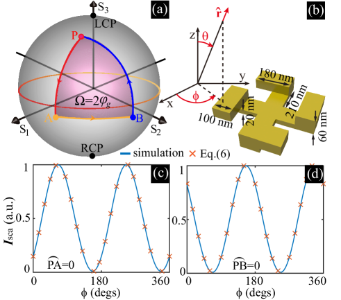
Figure 1: (a) Poincaré sphere on which P, A and B represent respectively the incident polarization and polarizations of the mode radiations opposite to the incident direction. The geometric phase is half solid angle of the orientated spherical triangle $\Delta\rm{PAB}$: $\varphi_{g}=\frac{1}{2}\Omega$. (b) A gold particle with 4-fold rotation symmetry and a spherical coordinate system parameterized by $\mathbf{r}=(r,~{}\theta,~{}\phi)$. Scattering intensity distributions on the $\mathbf{x}$-$\mathbf{y}$ plane: (c) P overlaps with A; (d) P overlaps with B.

After visualizing the excitation amplitude, now we turn to the phase $\varphi(\mathbf{\hat{r}})$ which can be generally categorized into two parts:

$$\varphi(\mathbf{\hat{r}})=\varphi_{g}+\varphi_{j}(\mathbf{\hat{r}}).$$ (5)

Here $\varphi_{g}$ is the global scattering direction $\mathbf{\hat{r}}$-independent geometric phase $\varphi_{g}=\frac{1}{2}\Omega$, where $\Omega$ denotes the solid angle enclosed by the great-arc circuit A PABP [see Fig. 1(a); $\Omega$ is positive (negative) for counter-clockwise (clockwise) circuit viewed above] [29, 30, 31, 32]. The other term $\varphi_{j}(\mathbf{\hat{r}})$ is the local $\mathbf{\hat{r}}$-dependent phase difference between the directional radiations: $\varphi_{j}(\mathbf{\hat{r}})=\rm{Arg}[\mathbb{J}_{\rm{A}}\mathbb{J}^{\dagger}_{\rm{B}}]$. Since the overall phase for each QNM (and thus also their Jones vectors) can be arbitrarily chosen, $\varphi_{j}$ seems to be indeterminate due to the gauge freedom of adding an arbitrary extra constant phase term $\Delta\varphi$ [32]: $\varphi_{j}(\mathbf{\hat{r}})\mapsto\varphi_{j}(\mathbf{\hat{r}})+\Delta\varphi$. In contrast, the geometric phase term is gauge-independent and has nothing to do with the overall assigned phase to each QNM (the position of Jones vector on the Poincaré sphere is irrelevant to its overall phase). Such phase indeterminacy (gauge freedom) can be fixed by the optical theorem, which imposes a stringent constraint on both the phase and amplitude of the forward scattering $\mathbf{E}_{\rm{sca}}(\mathbf{\hat{r}}_{\rm{inc}})$ [1]. Alternatively, $\Delta\varphi$ can be quickly decided through a single fitting of Eq. (4) with numerically calculated results. This $\Delta\varphi$ obtained can then be used for any incident polarizations, though generally it is dependent on the incident direction, along which the optical theorem imposes its constraint. For a fixed incident direction, $\Delta\varphi$ can be gauged out by assigning to modes A and B an equal constant relative phase, and then Eq. (1) can be simplified as (for two QNMs):

$$\mathbf{E}_{\rm{sca}}(\mathbf{\hat{r}})\propto\cos(\frac{1}{2}{\ooalign{\leavevmode\resizebox{13.47224pt}{0.0pt}{{\phantom{A}}}\cr PA}})~{}{\mathbf{E}}_{\rm{A}}(\mathbf{\hat{r}})+\cos(\frac{1}{2}{\ooalign{\leavevmode\resizebox{13.88893pt}{0.0pt}{{\phantom{A}}}\cr PB}})~{}{\mathbf{E}}_{\rm{B}}(\mathbf{\hat{r}})\exp({i\varphi_{g}}),$$ (6)

through which the distributions of not only intensities but also polarizations can be directly calculated.

Though the geometric phase has already been widely employed for various photonic functionalities [39, 40, 41], our theoretical framework and formulism are profoundly different, being both deeper and broader: (i) Previous studies are mostly based on structures consisting of optical items with spatially varying orientations, where the geometric phase emerges among the modes of individual items (the near-field couplings between them are thus neglected) and the formulism is valid only for a limited range of incident directions and polarizations. Here we discuss the optical structure (could be an individual particle or their clusters) as a whole and the geometric phase emerges among different QNMs of the same structure. As a result, our model has automatically considered all sorts of couplings and our formulism can accommodate arbitrary incident directions and polarizations; (ii) As we have revealed, what essentially decide the geometric phase are not geometric orientations of optical structures, but rather the polarization orientations (and also ellipticities) of the mode radiations opposite to the incident direction. The former is a good approximation only for some special scenarios, e.g. each item supports solely an electric dipole along its orientation direction and the incident direction is perpendicular to it, as is indeed the case for many previous demonstrations. As a result, the previously widely-adopted approach to directly associate geometric phase with the structure orientation is a reduced approximation of our model.

We now turn to a specific scattering particle shown in Fig. 1(b) to verify our theoretical framework (numerical calculations are performed using COMSOL Multiphysics throughout this work). The particle consists of gold (effective permittivity fitted from data in Ref. [42]) and exhibits four-fold rotation symmetry that secures a pair of degenerate QNMs with central resonant angular frequency $\omega_{1}=8.0645\times 10^{14}~{}\rm{rad}/s$. We shine plane waves along $\mathbf{+z}$ with $\omega=\omega_{1}$ and track scattering distributions on the $\mathbf{x}$-$\mathbf{y}$ plane, unless specified otherwise. For other off-resonance frequencies, as long as no other modes are excited, scattering distributions would be the same as the relative amplitude and phase are independent of frequency detuning due to mode degeneracy. The radiations of the two QNMs along -$\mathbf{z}$ (opposite to the incident direction) are almost linearly polarized along $\mathbf{x}$ and $\mathbf{y}$, with the corresponding normalized Stokes parameters [33] being respectively $S_{1}\approx\pm 1$ [see points A and B in Fig. 2(b)]. The normalized scattering intensity distributions on the $\mathbf{x}$-$\mathbf{y}$ plane [parameterized by the azimuthal angle $\phi$ as shown in Fig. 1(b)] are shown in Fig. 1(c) and 1(d), for incident linear polarizations along $\mathbf{x}$ (${\ooalign{\leavevmode\resizebox{13.47224pt}{0.0pt}{{\phantom{A}}}\cr PA}}\approx 0$, ${\ooalign{\leavevmode\resizebox{13.88893pt}{0.0pt}{{\phantom{A}}}\cr PB}}\approx\pi$ and thus mode B is not excited: $I_{\rm{sca}}\propto I_{\rm{A}}$) and $\mathbf{y}$ (${\ooalign{\leavevmode\resizebox{13.88893pt}{0.0pt}{{\phantom{A}}}\cr PB}}\approx 0$, ${\ooalign{\leavevmode\resizebox{13.47224pt}{0.0pt}{{\phantom{A}}}\cr PA}}\approx\pi$ and thus mode A is not excited: $I_{\rm{sca}}\propto I_{\rm{B}}$), respectively. As is clearly shown in Fig. 1(c) and 1(d), radiations of modes A and B [$I_{\rm{A,B}}(\phi)$] agree well with the directly simulated intensity distributions without involving QNMs, confirming the accuracy of our model and also that by properly selecting the incident polarizations, modes can be selectively excited as long as A and B do not overlap.

The scattering intensity distributions for two other incident orthogonal linear polarizations [polarized along $\phi=\pi/4$ ($S_{2}=1$) and polarized along $\phi=3\pi/4$ ($S_{2}=-1$); see positions of P in Fig. 2(b)] are summarized in Fig. 2(a). For both scenarios ${\ooalign{\leavevmode\resizebox{13.47224pt}{0.0pt}{{\phantom{A}}}\cr PA}}\approx{\ooalign{\leavevmode\resizebox{13.88893pt}{0.0pt}{{\phantom{A}}}\cr PB}}\approx\pi/2$, and the core difference is that for the former $\varphi_{g}\approx 0$ while for the latter $\varphi_{g}\approx\pi$ [see Fig. 2(b)], leading to fully distinct scattering distributions $I_{\rm{sca}}\propto I_{\rm{A}}+I_{\rm{B}}\pm 2\sqrt{I_{\rm{A}}I_{\rm{B}}}|\mathbb{J}_{\rm{A}}\mathbb{J}_{\rm{B}}^{\dagger}|\cos[\varphi_{j}(\mathbf{\hat{r}})]$. The geometric phase $\pi$ is directly manifest through the two distinct curves shown in Fig. 2(a). We note that our demonstration (with an individual scattering particle) of such classical geometric phase $\pi$ is even simpler and more direct than the earliest ones by Fresnel-Arago and Hamilton-Lloyd [32]. Results for two other scenarios with fixed ${\ooalign{\leavevmode\resizebox{13.47224pt}{0.0pt}{{\phantom{A}}}\cr PA}}\approx{\ooalign{\leavevmode\resizebox{13.88893pt}{0.0pt}{{\phantom{A}}}\cr PB}}\approx\pi/2$ but different geometric phases [Fig. 2(b)] of $\varphi_{g}\approx\pi/2$ [left-handed circular polarization (LCP) incidence with $S_{3}=1$] and $\varphi_{g}\approx\pi/4$ [elliptic polarization with P locating at ($0$, $\sqrt{2}/2$, $\sqrt{2}/2$)] are summarized in Fig. 2(c), where the influence of geometric phase is also apparent. As is shown in Fig. 2(a), for $\varphi_{g}\approx 0$ the scattering along the direction $\phi=\phi_{0}\approx 113^{\circ}$ is zero. Along this direction, Eq. (4) can be reduced to $I_{\rm{sca}}(\phi=\phi_{0})\propto 1-\cos(\varphi_{g})$ as long as ${\ooalign{\leavevmode\resizebox{13.47224pt}{0.0pt}{{\phantom{A}}}\cr PA}}\approx{\ooalign{\leavevmode\resizebox{13.88893pt}{0.0pt}{{\phantom{A}}}\cr PB}}\approx\pi/2$. We then show the evolutions of $I_{\rm{sca}}(\phi=\phi_{0})$ on such a polarization great circle ($S_{1}=0$) parameterized by $\beta\in[0,2\pi]$, as shown in the inset in Fig. 2(d). Obviously the solid angle $\Omega=2\beta$ and $\varphi_{g}=\beta$ [Fig. 2(b)], and thus the evolution observe the relation $I_{\rm{sca}}(\phi=\phi_{0})\propto 1-\cos(\beta)$, which agrees perfectly with the numerical results included in Fig. 2(d).

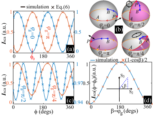
Figure 2: Scattering intensity distributions on the $\mathbf{x}$-$\mathbf{y}$ plane with P locating at ($0$, $1$, $0$) and ($0$, $-1$, $0$) for (a); ($0$, $0$, $1$) and ($0$, $\sqrt{2}/2$, $\sqrt{2}/2$) for (c). The geometric phase are respectively $\varphi_{g}=0,\pi,\pi/2$ and $\pi/4$, as shown in (b). In (a) one diretion of zero scattering $\phi=\phi_{0}\approx 113^{\circ}$ is specified. (d) The dependence of $I_{\rm{sca}}(\phi=\phi_{0})$ on $\beta$ that parameterizes a great circle ($S_{1}=0$) on the Poincaré sphere (see the inset).

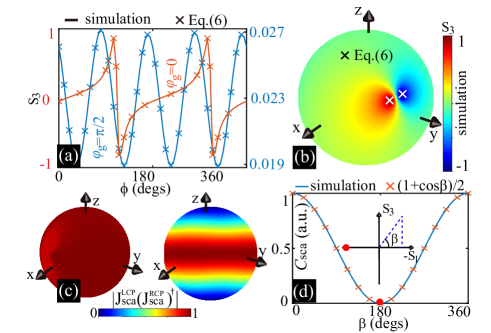
Figure 3: (a) $S_{3}$ distributions on the $\mathbf{x}$-$\mathbf{y}$ plane with P locating at ($0$, $0$, $1$) and ($0$, $1$, $0$), with $\varphi_{g}=\pi/2$ and $0$, respeively. (b) $S_{3}$ distributions on the whole scattering momentum sphere for P locating at ($0$, $1$, $0$), on which the predicted directions of cirular polarization singularities are marked by crosses. (c) Distributions of $|\mathbf{J}_{\rm{sca}}^{\rm{LCP}}(\mathbf{J}_{\rm{sca}}^{\rm{RCP}})^{\dagger}|$ for waves incident along $\mathbf{\hat{r}}_{\rm{inc}}=-\mathbf{\hat{r}}_{\rm{A=B}}$ (left) and $\mathbf{\hat{r}}_{\rm{inc}}=\mathbf{+z}$ (right). (d) Variations of $C_{\rm{sca}}$ for P transversing a great circle ($S_{2}=0$), covering matched polarization ($\beta=0$), orthogonal polarization (marked; $\beta=\pi$), LCP and RCP ($\beta=\pi/2$ and $3\pi/2$).

Our theoretical framework can predict the distributions of not only scattering intensities according to Eq. (4), but also of polarizations according to Eq. (6). The polarization distributions (in terms of $S_{3}$ of the scattered fields) on the $\mathbf{x}$-$\mathbf{y}$ plane are shown in Fig. 3(a), for linear polarization ($S_{2}=1$ and $\varphi_{g}\approx 0$) and LCP ($S_{3}=1$ and $\varphi_{g}\approx\pi/2$) incidences, where the agreement further confirms the accuracy of our theoretical framework. According to Eq. (6), the locations of circularly-polarized scatterings ($S_{3}=\pm 1$; circular polarization singularities [13]) can be directly predicted and even designed by selecting proper incident polarization and directions. We show the scattering polarization distributions (simulated results) on the whole scattering momentum sphere in Fig. 3(b) for the linear polarization incidence ($S_{2}=1$) and the predicted locations of polarization singularities are also marked by crosses, agreeing well with the numerical calculations.

According to Eq. (6), there is a rather interesting scenario of overlapped A and B: directions where the radiation polarizations for both QNMs are the same, with $\cos(\frac{1}{2}{\ooalign{\leavevmode\resizebox{13.47224pt}{0.0pt}{{\phantom{A}}}\cr PA}})=\cos(\frac{1}{2}{\ooalign{\leavevmode\resizebox{13.88893pt}{0.0pt}{{\phantom{A}}}\cr PB}})$ and $\varphi_{g}=0$ [see Fig. 1(a)]. For waves incident opposite to those directions, along any scattering direction the polarization would not change, irrespective of the incident polarization. For the marked direction ($\phi=\phi_{0}$) in Fig. 2(a) where the scattering is zero, since both modes are excited, along this direction mode radiation polarization must be the same or they would not cancel each other. This is also the requirement of Eq. (4), as $I_{\rm{sca}}=0$ requires $|\mathbb{J}_{\rm{A}}\mathbb{J}_{\rm{B}}^{\dagger}=1|$ which means an identical radiation polarization. We denote this direction as $\mathbf{\hat{r}}_{\rm{A=B}}$ and shine opposite to it ($\mathbf{\hat{r}}_{\rm{inc}}=-\mathbf{\hat{r}}_{\rm{A=B}}$) plane waves of LCP and RCP (left-handed circular polarization). We then track the scattering polarization variation on the whole momentum sphere through the parameter $|\mathbf{J}_{\rm{sca}}^{\rm{LCP}}(\mathbf{J}_{\rm{sca}}^{\rm{RCP}})^{\dagger}|$, where $|\mathbf{J}_{\rm{sca}}^{\rm{LCP}}(\mathbf{J}_{\rm{sca}}^{\rm{RCP}})^{\dagger}|=1$ means the scattering polarization does not change for RCP and LCP incidences [see Fig. 3(c)]. Here $\mathbf{J}_{\rm{sca}}$ denotes the normalized Jones vector for the scattered expressed by Eq. (6), and its superscript indicates the incident polarization. For comparison, we also shine circularly-polarized waves along +$\mathbf{z}$ (where A and B do not overlap) and show its $|\mathbf{J}_{\rm{sca}}^{\rm{LCP}}(\mathbf{J}_{\rm{sca}}^{\rm{RCP}})^{\dagger}|$ distribution in Fig. 3(c), confirming that for general incident directions the scattering polarizations are dependent on incident polarizations.

Another interesting property for overlapped A and B is that the incident polarization can be tuned to be orthogonal to that of both QNMs [$\cos(\frac{1}{2}{\ooalign{\leavevmode\resizebox{13.47224pt}{0.0pt}{{\phantom{A}}}\cr PA}})=\cos(\frac{1}{2}{\ooalign{\leavevmode\resizebox{13.88893pt}{0.0pt}{{\phantom{A}}}\cr PB}})=0$]. For such an incident polarization, neither QNM would be excited and thus the particle would become invisible. For the same incident direction ($\mathbf{\hat{r}}_{\rm{inc}}=-\mathbf{\hat{r}}_{\rm{A=B}}$), we show the evolutions of scattering cross sections ($C_{\rm{sca}}$) with varying incident polarizations in Fig. 3(d). The incident polarization covers a great circle, covering matched polarization ($\beta={\ooalign{\leavevmode\resizebox{13.47224pt}{0.0pt}{{\phantom{A}}}\cr PA}}={\ooalign{\leavevmode\resizebox{13.88893pt}{0.0pt}{{\phantom{A}}}\cr PB}}=0$), LCP ($\beta=\pi/2$), orthogonal polarization ($\beta={\ooalign{\leavevmode\resizebox{13.47224pt}{0.0pt}{{\phantom{A}}}\cr PA}}={\ooalign{\leavevmode\resizebox{13.88893pt}{0.0pt}{{\phantom{A}}}\cr PB}}=\pi$). According to Eq. (4), scattering along any direction and thus also the scattering cross section would adhere to $I_{\rm{sca}},C_{\rm{sca}}~{}\propto 1+\cos(\beta)$, which is verified by Fig. 3(d). We note that the scattering evolutions in Fig. 2(d) are driven by changing $\varphi_{g}$ with ${\ooalign{\leavevmode\resizebox{13.47224pt}{0.0pt}{{\phantom{A}}}\cr PA}}={\ooalign{\leavevmode\resizebox{13.88893pt}{0.0pt}{{\phantom{A}}}\cr PB}}$ fixed at $\pi/2$, while those in Fig. 3(d) driven by changing ${\ooalign{\leavevmode\resizebox{13.47224pt}{0.0pt}{{\phantom{A}}}\cr PA}}={\ooalign{\leavevmode\resizebox{13.88893pt}{0.0pt}{{\phantom{A}}}\cr PB}}$, with $\varphi_{g}$ fixed at $0$.

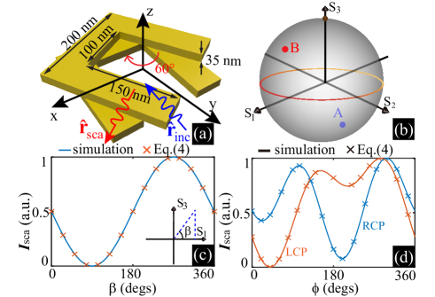
Figure 4: (a) A pair of gold split-ring resonators, and two directions of interest ($\mathbf{\hat{r}}_{\rm{sca}}$ and $\mathbf{\hat{r}}_{\rm{inc}}$) are also marked. The corresponding A $(-0.29,-0.41,-0.86)$ and B $(0.38,-0.81,0.45)$ for this $\mathbf{\hat{r}}_{\rm{inc}}$ are shown in (b). The dependence of the directional scattering intensity along $\mathbf{\hat{r}}_{\rm{sca}}$ on incident polarizations is shown in (c), with P transversing a great circle on the Poincaré sphere ($S_{2}=0$), covering LCP ($\beta=\pi/2$) and RCP ($\beta=3\pi/2$). (d) Scattering intensity distributions on the $\mathbf{x}$-$\mathbf{y}$ plane with LCP and RCP incidences along the marked incident direction.

So far we have showcased only the scenario of two degenerate QNMs while our theoretical framework does not require such degeneracy. For non-degenerate QNMs, deviations from the central resonant positions would only shift the overall phase and amplitude of the corresponding QNM radiations [27], the effect of which can be taken into consideration in our model by adjusting the corresponding excitation coefficients accordingly, with the geometric phase term unaffected. We have further studied a scattering structure shown in Fig. 4(a), which supports a pair of non-degenerate QNMs with central resonant frequencies close to $\omega_{2}=1.1695\times 10^{15}~{}\rm{rad}/s$, at which the angular frequency of the incident wave is fixed ($\omega=\omega_{2}$). We have identified a scattering direction $\mathbf{\hat{r}}_{\rm{sca}}$ ($\phi=41^{\circ}$ and $\theta=90^{\circ}$; on the $\mathbf{x}$-$\mathbf{y}$ plane) along which the radiation polarizations of both QNMs are identical. As has already been elaborated, through tuning the relative exciting amplitude and phase, scattering along this direction can be eliminated, similar to that marked in Fig. 2(a). We have selected an incident direction $\mathbf{\hat{r}}_{\rm{inc}}$ ($\phi=0$ and $\theta=10^{\circ}$) and the corresponding positions of A and B are shown in Fig. 4(b). The evolution of the directional scattering intensity along $\mathbf{\hat{r}}_{\rm{sca}}$ with changing incident polarizations covering a great circle ($S_{2}=0$) is shown in Fig. 4(c), where the scattering is fully suppressed for LCP incidence ($\beta=\pi/2$). We have also tracked the scattering intensity distributions on the $\mathbf{x}$-$\mathbf{y}$ plane for LCP and RCP incidences, with the results summarized in Fig. 4(d).

In conclusion, we have unveiled the hidden excitation geometric phases among QNMs of scatterers and reveal how they drive scattering evolutions on the incident Poincaré sphere. The geometric phase can be exploited to efficiently manipulate the scatterings, such as scattering eliminations and polarization singularity (zero and circularly-polarized scatterings) generations. For the general scenario of more than two QNMs being simultaneously excited, the relative amplitude and phase among any two QNMs can be calculated using our model and then calculations for interferences among all QNMs become routine. This means that the theoretical framework we have constructed is generic and widely applicable. We have essentially merged three vibrant fields of geometric phase, Mie scattering and QNM, and unlocked an extra hidden dimension of electromagnetic scattering. Similar dimensions might be uncovered for waves of other forms for which geometric phase is generic and ubiquitous, providing new flexibilities for many physics and interdisciplinary branches that are related to wave scatterings.

Acknowledgment: This work is supported by National Natural Science Foundation of China (Grant No. 11874426 and 61405067), and several Researcher Schemes of National University of Defense Technology. W. L. acknowledges many illuminating correspondences with Sir Michael Berry, whose monumental paper on geometric phase was published $40$ years ago today.

References

- [1] C. F. Bohren and D. R. Huffman, Absorption and Scattering of Light by Small Particles (Wiley, 1983).
- [2] A. I. Kuznetsov, A. E. Miroshnichenko, M. L. Brongersma, Y. S. Kivshar, and B. Luk'yanchuk, ``Optically resonant dielectric nanostructures,'' Science 354, aag2472 (2016).
- [3] W. Liu and Y. S. Kivshar, ``Generalized Kerker effects in nanophotonics and meta-optics [Invited],'' Opt. Express 26, 13085–13105 (2018).
- [4] A. Krasnok, D. Baranov, H. Li, M.-A. Miri, F. Monticone, and A. Alú, ``Anomalies in light scattering,'' Adv. Opt. Photon. 11, 892–951 (2019).
- [5] Y. Kivshar, ``The Rise of Mie-tronics,'' Nano Lett. 22, 3513–3515 (2022).
- [6] H. Altug, S.-H. Oh, S. A. Maier, and J. Homola, ``Advances and applications of nanophotonic biosensors,'' Nat. Nanotechnol. 17, 5–16 (2022).
- [7] S. Fan and W. Li, ``Photonics and thermodynamics concepts in radiative cooling,'' Nat. Photon. 16, 182–190 (2022).
- [8] S. Pancharatnam, ``The propagation of light in absorbing biaxial crystals,'' Proc. Indian. Acad. Sci. 42, 86–109 (1955).
- [9] M. Berry, ``Pancharatnam, virtuoso of the Poincaré sphere: An appreciation,'' Curr. Sci. 67, 220–220 (1994).
- [10] T. Ozawa, H. M. Price, A. Amo, N. Goldman, M. Hafezi, L. Lu, M. C. Rechtsman, D. Schuster, J. Simon, O. Zilberberg, and I. Carusotto, ``Topological photonics,'' Rev. Mod. Phys. 91, 015006 (2019).
- [11] C. Wang, Z. Fu, W. Mao, J. Qie, A. D. Stone, and L. Yang, ``Non-Hermitian optics and photonics: From classical to quantum,'' Adv. Opt. Photon., AOP 15, 442–523 (2023).
- [12] C. W. Hsu, B. Zhen, A. D. Stone, J. D. Joannopoulos, and M. Soljačić, ``Bound states in the continuum,'' Nat. Rev. Mater. 1, 16048 (2016).
- [13] G. J. Gbur, Singular Optics (CRC Press Inc, Boca Raton, 2016).
- [14] W. Liu, W. Liu, L. Shi, and Y. Kivshar, ``Topological polarization singularities in metaphotonics,'' Nanophotonics 10, 1469–1486 (2021).
- [15] M.-A. Miri and A. Alù, ``Exceptional points in optics and photonics,'' Science 363, eaar7709 (2019).
- [16] K. Koshelev, A. Bogdanov, and Y. Kivshar, ``Meta-optics and bound states in the continuum,'' Science Bulletin 64, 836–842 (2019).
- [17] M. Kang, T. Liu, C. T. Chan, and M. Xiao, ``Applications of bound states in the continuum in photonics,'' Nat Rev Phys 5, 659–678 (2023).
- [18] A. Doicu, T. Wriedt, and Y. A. Eremin, Light Scattering by Systems of Particles: Null-Field Method with Discrete Sources: Theory and Programs, vol. 124 (Springer, 2006).
- [19] T. Needham, Visual Differential Geometry and Forms: A Mathematical Drama in Five Acts (Princeton University Press, Princeton, 2021).
- [20] W. Liu, J. Zhang, B. Lei, H. Ma, W. Xie, and H. Hu, ``Ultra-directional forward scattering by individual core-shell nanoparticles,'' Opt. Express 22, 16178 (2014).
- [21] J. D. Jackson, Classical Electrodynamics Third Edition (Wiley, New York, 1998), 3rd ed.
- [22] W. Liu, ``Generalized magnetic mirrors,'' Phys. Rev. Lett. 119, 123902 (2017).
- [23] W. Chen, Y. Chen, and W. Liu, ``Singularities and Poincaré indices of electromagnetic multipoles,'' Phys. Rev. Lett. 122, 153907 (2019).
- [24] W. Chen, Y. Chen, and W. Liu, ``Line Singularities and Hopf Indices of Electromagnetic Multipoles,'' Laser Photonics Rev. 14, 2000049 (2020).
- [25] I. Fernandez-Corbaton, X. Zambrana-Puyalto, N. Tischler, X. Vidal, M. L. Juan, and G. Molina-Terriza, ``Electromagnetic Duality Symmetry and Helicity Conservation for the Macroscopic Maxwell's Equations,'' Phys. Rev. Lett. 111, 060401 (2013).
- [26] Q. Yang, W. Chen, Y. Chen, and W. Liu, ``Electromagnetic Duality Protected Scattering Properties of Nonmagnetic Particles,'' ACS Photonics 7, 1830–1838 (2020).
- [27] P. Lalanne, W. Yan, K. Vynck, C. Sauvan, and J.-P. Hugonin, ``Light Interaction with Photonic and Plasmonic Resonances,'' Laser Photonics Rev. 12, 1700113 (2018).
- [28] C. Caloz, A. Alù, S. Tretyakov, D. Sounas, K. Achouri, and Z.-L. Deck-Léger, ``Electromagnetic Nonreciprocity,'' Phys. Rev. Applied 10, 047001 (2018).
- [29] S. Pancharatnam, ``Generalized theory of interference, and its applications,'' Proc. Indian. Acad. Sci. 44, 247–262 (1956).
- [30] M. V. Berry, ``Quantal Phase Factors Accompanying Adiabatic Changes,'' Proc. R. Soc. A 392, 45–57 (1984).
- [31] M. V. Berry, ``The Adiabatic Phase and Pancharatnam Phase for Polarized-Light,'' J. Mod. Opt. 34, 1401 (1987).
- [32] M. Berry, ``A Geometric-Phase Timeline,'' Optics & Photonics News 3, 42–49 (2024).
- [33] A. Yariv and P. Yeh, Photonics: Optical Electronics in Modern Communications (Oxford University Press, New York, 2006), 6th ed.
- [34] W. Chen, Q. Yang, Y. Chen, and W. Liu, ``Extremize Optical Chiralities through Polarization Singularities,'' Phys. Rev. Lett. 126, 253901 (2021).
- [35] G. N. Ramachandran and S. Ramaseshan, ``Crystal Optics,'' in ``Kristalloptik Beugung/Crystal Optics Diffraction,'' , S. Flügge, ed. (Springer, Berlin, Heidelberg, 1961), Handbuch Der Physik / Encyclopedia of Physics, pp. 1–217.
- [36] S. Pancharatnam, Collected Works of S. Pancharatnam (Oxford University Press for the Raman Research Institute, London, 1975).
- [37] M. V. Berry, ``The adiabatic phase and pancharatnam phase for polarized-light,'' J. Mod. Opt. 34, 1401 (1987).
- [38] C. Wen, J. Zhang, S. Qin, Z. Zhu, and W. Liu, ``Momentum-Space Scattering Extremizations,'' Laser & Photonics Reviews 18, 2300454 (2024).
- [39] G. Li, S. Zhang, and T. Zentgraf, ``Nonlinear photonic metasurfaces,'' Nat. Rev. Mater. 2, 17010 (2017).
- [40] E. Cohen, H. Larocque, F. Bouchard, F. Nejadsattari, Y. Gefen, and E. Karimi, ``Geometric phase from Aharonov–Bohm to Pancharatnam–Berry and beyond,'' Nat. Rev. Phys. 1, 437–449 (2019).
- [41] C. P. Jisha, S. Nolte, and A. Alberucci, ``Geometric Phase in Optics: From Wavefront Manipulation to Waveguiding,'' Laser & Photonics Reviews 15, 2100003 (2021).
- [42] P. B. Johnson and R. W. Christy, ``Optical constants of the noble metals,'' Phys. Rev. B 6, 4370 (1972).