Non-Abelian Exponential Yang-Mills AdS Black Brane and Transport Coefficients

Abstract

In this paper, AdS black brane solution of Einstein-Hilbert gravity with non-abelian exponential guage theory of Yang-Mills type is introduced. DC conductivity and the ratio of shear viscosity to entropy density as two important transport coefficients are calculated by using of Kubo formula in the context of AdS/CFT duality. Our results recover the Yang-Mills model in $q\to\infty$ limit.

PACS numbers: 11.10.Jj, 11.10.Wx, 11.15.Pg, 11.25.Tq

Keywords: Black brane, AdS/CFT duality, Non-abelian color DC conductivity, Shear viscosity

1 Introduction

Quantum chromodynamics (QCD) as a non-abelian gauge theory with $SU(3)$ symmetry group describes the strong interaction between quarks mediated by gluons. The strong interaction can be described through the Yang-Mills theory with the Lagrangian density, ${\bf{Tr}}(F_{\mu\nu}^{(a)}F^{(a)\,\,\mu\nu})$. The Yang-Mills theory is a nonlinear theory and it suffers from problems such as singularity on the point like charge and infinite self-energy [1, 2, 3]. The Lagrangian of nonlinear Yang-Mills field has been considered in various theories of gravity. The generalization of Yang-Mills black holes plays a crucial role since most of physical systems are intrinsically nonlinear in the nature which leads to revelation of some loop corrections.

The Einstein-Yang-Mills AdS black brane [4] is a solution of Einstein-Yang-Mills gravity with the flat topology of event horizon. The generalization of this solution is studied in various gravity theories like Gauss-Bonnet massive gravity[5] and higher derivative massive gravity[6] to explain inflation and current acceleration of the Universe [7]-[10] and some aspects of quantum gravity.

Logarithmic gauge theory [11],[12],[13], arcsin-electrodynamics [14],[15], Born-Infeld theory [16, 17] have been introduced as nonlinear theories (NED) to solve some of problems in Yang-Mills theory. The NED fields give more information in higher magnetized neutron stars and pulsars [18][19]. These theories remove both of big-bang and black hole singularities [20]-[21] by modifying spacetime geometry.

There are three kinds of Born-Infeld (BI) actions, Born-Infeld nonlinear electromagnetic (BINEF), logarithmic form of nonlinear electromagnetic field (LNEF) and exponential form of nonlinear electromagnetic field (ENEF)[22].

$$L(\mathcal{F})=\left\{\begin{array}[]{cc}4q^{2}\bigg{(}1-\sqrt{1+\frac{\mathcal{F}}{2q^{2}}}\bigg{)}&\text{BINEF}\\ q^{2}\bigg{(}exp({-\frac{\mathcal{F}}{q^{2}}})-1\bigg{)}&\text{ENEF}\\ -8q^{2}\ln\bigg{(}1+\frac{\mathcal{F}}{8q^{2}}\bigg{)}&\text{LNEF}.\\ \end{array}\right.$$ (1)

These Lagrangian functions tends to the Yang-Mills Lagrangian functions when, $q\to\infty$. A good question that can be asked is, what is the need to introduce these nonlinear models?. Why is the specific nonlinear YM action (ENEF) chosen among other options?. To answer these questions, we consider that above Lagrangian functions can be expanded as following general form,

$$\mathcal{L}=-\mathcal{F}+\alpha\mathcal{F}^{2}+\beta\mathcal{F}^{3}+\gamma\mathcal{F}^{4}+...\,\,\,.$$ (2)

Here, $\alpha$ , $\beta$ and $\gamma$ are the general constant coefficients and $\mathcal{F}=F_{\mu\nu}F^{\mu\nu}$. For each of above functions, the expansion coefficients are different. So, we have:

$$L(\mathcal{F})=\left\{\begin{array}[]{cc}4q^{2}\bigg{(}1-\sqrt{1+\frac{\mathcal{F}}{2q^{2}}}\bigg{)}=-\mathcal{F}+\frac{\mathcal{F}^{2}}{8q^{2}}-\frac{\mathcal{F}^{3}}{32q^{4}}+\frac{5\mathcal{F}^{4}}{512q^{6}}-\frac{7\mathcal{F}^{5}}{2048q^{8}}+...&\text{BINEF}\\ q^{2}\bigg{(}exp({-\frac{\mathcal{F}}{q^{2}}})-1\bigg{)}=-\mathcal{F}+\frac{\mathcal{F}^{2}}{2q^{2}}-\frac{\mathcal{F}^{3}}{6q^{4}}+\frac{\mathcal{F}^{4}}{24q^{6}}-\frac{\mathcal{F}^{5}}{120q^{8}}+...&\text{ENEF}\\ -8q^{2}\ln\bigg{(}1+\frac{\mathcal{F}}{8q^{2}}\bigg{)}=-\mathcal{F}+\frac{\mathcal{F}^{2}}{16q^{2}}-\frac{\mathcal{F}^{3}}{192q^{4}}+\frac{\mathcal{F}^{4}}{2048q^{6}}-\frac{\mathcal{F}^{5}}{20480q^{8}}+...&\text{LNEF}.\\ \end{array}\right.$$ (3)

The general behavior of these functions may be the same, but they differ in details. Different expansion coefficients can help us to describe the cosmic inflation periods and match the observational results [22],[23]. Therefore, examining each of the functions allows us to test our luck in finding an explanatory optimal higher derivative YM models that match the observations.

The color DC conductivity bound of Einstein–Born–Infeld AdS black brane was studied in [24] and the same method for logarithmic form of Born-Infeld (BI) action was considered in [13]. We consider the exponential form of nonlinear Yang-Mills in this paper.

Fluid-gravity duality [25]-[30] is a version of AdS/CFT duality[31] for long wavelength limit. The boundary theory behaves as a fluid effectively and hydrodynamics equations which are conserved charges up to first order of derivative expansion are as follows,

$$\nabla_{\mu}J^{\mu}=0\,\,\,\,\,,\,\,\nabla_{\mu}T^{\mu\nu}=0,$$ (4)

$$J^{\mu}=n\,u^{\mu}-\sigma TP^{\mu\nu}\partial_{\nu}(\frac{\mu}{T}),$$

$$T^{\mu\nu}=(\rho+p)u^{\mu}u^{\nu}+pg^{\mu\nu}-\sigma^{\mu\nu},$$

$$\sigma^{\mu\nu}={P^{\mu\alpha}P^{\nu\beta}}[\eta(\nabla_{\alpha}u_{\beta}+\nabla_{\beta}u_{\alpha})+(\zeta-\frac{2}{3}\eta)g_{\alpha\beta}\nabla.u],$$

$$P^{\mu\nu}=g^{\mu\nu}+u^{\mu}u^{\nu},$$

where $n$, $\eta$, $\zeta$, $\sigma^{\mu\nu}$ , $\sigma$ and $P^{\mu\nu}$ are charge density, shear viscosity, bulk viscosity, shear tensor, conductivity and projection operator, respectively [27]. $\eta$, $\zeta$ and $\sigma$ are known as transport coefficients.
Green-Kubo formula relates transport coeffeicnts to two-point function [25] as follows,

$$\sigma^{(ab)}_{ij}(k_{\mu})=-\mathop{\lim}\limits_{\omega\to 0}\frac{1}{\omega}\Im G^{(ab)}_{ij}(k_{\mu}).$$ (5)

Where lower and upper indices refer to the spatial directions and gauge group, respectively. There is a universal bound for DC conductivity as $\sigma\geq\frac{1}{e^{2}}$ where $e$ is the charge of the gauge field. This bound is also saturated in graphene[32], but it is violated for massive gravity [33], models with abelian case [34] and non-abelian Born-Infeld theory[24].
Another important quantity in Quak-Gloun-Plasma (QGP) or systems with strong coupling is the ratio of shear viscosity to entropy density i.e. $\frac{\eta}{s}\geq\frac{\hbar}{4\,\pi\,k_{B}}$, called the Kovtun-Son-Starinet (KSS) bound [35]. The KSS bound is saturated for Einstein-Hilbert gravity but it is violated for Horndeski theory [36], massive gravity for $c_{i}<0$ [37], scalar-tensor gravity[38]-[40], anisotropic black brane [41], Gauss–Bonnet massive gravity[5], deformed $AdS_{4}$–Reissner–Nordström [42], AdS₅-Schwarzschild deformed black branes[43], higher curvature massive gravity[6] and massive gravity [44]. The quantity $\frac{\eta}{s}$ is proportional to the inverse of the square of the field theory coupling i.e. $\frac{\eta}{s}\sim\frac{1}{\lambda^{2}}$.
In this paper, we want to study the DC conductivity and $\frac{\eta}{s}$ for non-abelian exponential Yang-Mills AdS black brane to describe the field theory dual of this model.

2 Non-Abelian Exponential Yang-Mills AdS Black Brane

The 4-dimensional action of non-abelian exponential gauge theory with negative cosmological constant is as follows[22],

$$S=\int d^{4}x\sqrt{-g}\bigg{[}R-2\Lambda-q^{2}\big{(}e^{-\frac{\mathcal{F}}{q^{2}}}-1\big{)}\bigg{]},$$ (6)

where, $R$ is the Ricci scalar, $\Lambda=-\frac{3}{l^{2}}$ is the cosmological constant, $l$ is the AdS radius, $\mathcal{F}={\bf{Tr}}(F_{\mu\nu}^{(a)}F^{(a)\,\,\mu\nu})$ is the Yang-Mills invariant and $q$ is the nonlinear coupling constant. The trace element stands for ${\bf{Tr}}(.)=\sum_{i=1}^{3}(.).$
$F_{\mu\nu}^{(a)}$ is the $SU(2)$ Yang-Mills field strength tensor,

$$F_{\mu\nu}=\partial_{\mu}A_{\nu}-\partial_{\nu}A_{\mu}-i[A_{\mu},A_{\nu}],$$ (7)

in which the gauge coupling constant is taken equal to one, $A_{\nu}$’s are the $SU(2)$ gauge group Yang-Mills potentials. When $q\to\infty$ the exponential term gets transformed into standard linear non-abelian Yang-Mills term [45]. Einstein and Yang-Mills equations are obtained through the variation of the action (6) with respect to $g_{\mu\nu}$ and $A^{(a)}_{\nu}$ respectively. The results of variations are as follows,

$$R_{\mu\nu}-\tfrac{1}{2}g_{\mu\nu}R+\Lambda g_{\mu\nu}+\tfrac{1}{2}g_{\mu\nu}q^{2}\left(e^{-\frac{F_{\rho\beta}^{(a)}F^{(a)\,\,\rho\beta}}{q^{2}}}-1\right)-2F^{(a)}_{\mu\gamma}F^{(a)}_{\nu}\,{}^{\gamma}e^{-\frac{F_{\rho\beta}^{(a)}F^{(a)\,\,\rho\beta}}{q^{2}}}=0,$$ (8)

and

$$\nabla^{\mu}\bigg{(}e^{-\frac{F_{\rho\beta}^{(a)}F^{(a)\,\,\rho\beta}}{q^{2}}}F_{\mu\nu}^{(a)}\bigg{)}=0.$$ (9)

The covariant derivative is defined as,

$$\nabla_{\mu}=I\partial_{\mu}-ie\sigma^{(a)}A^{(a)}_{\mu},$$ (10)

here, $I$ represents the identity matrix and $\sigma^{(a)}$ represents the generators of $SU(2)$.
We want to introduce asymptotically AdS black brane solution in four dimensions in our model. So we consider the following ansatz,

$$ds^{2}=-f(r)dt^{2}+\frac{dr^{2}}{f(r)}+\frac{r^{2}}{l^{2}}(dx^{2}+dy^{2}),$$ (11)

where $f(r)$ is the blackening function which will be determined by solving Eq.(8). We consider the guage field ansatz as follows,

$${\bf{A}}^{(a)}=\frac{i}{\sqrt{2}}h(r)dt\begin{pmatrix}1&0\\ 0&-1\end{pmatrix}.$$ (12)

Here, $\sigma_{3}=\begin{pmatrix}1&0\\ 0&-1\end{pmatrix}$ is the generator of the $SU(2)$ symmetric group of the gauge field [45]. The non-zero component of Eq.(9) is as follows,

$$2q^{2}h^{\prime}(r)+r\Big{(}q^{2}+4h^{\prime}(r)^{2}\Big{)}h^{\prime\prime}(r)=0.$$ (13)

So, $h(r)$ is found as

$$h(r)=\mu+\int^{r}\frac{1}{2}q\sqrt{W[\frac{4e^{\frac{2C_{1}}{q^{2}}}}{q^{2}u^{4}}]}du,$$ (14)

where, $\mu$ is the constant of integration and is called chemical potential of quantum field theory that locates on the boundary of AdS spacetime in AdS/CFT duality. By applying regularity condition on the event horizon i.e. $A_{t}(r_{h})=0$ [46], we get,

$$\mu=-\int^{r_{h}}\frac{1}{2}q\sqrt{W[\frac{4e^{\frac{2C_{1}}{q^{2}}}}{q^{2}u^{4}}]}du.$$ (15)

Here $W$ is the Lambert function or omega function or product logarithm and $C_{1}$ is an integration constant which is related to the Yang-Mills charge.
The non-zero components of $F_{\mu\nu}^{(a)}$ are as follows,

$$F_{tr}^{(a)}=-F_{rt}^{(a)}=h^{\prime}(r)\begin{pmatrix}1&0\\ 0&-1\end{pmatrix}=-\frac{1}{2\sqrt{2}}q\sqrt{W\left(\frac{4e^{\frac{2C_{1}}{q^{2}}}}{q^{2}r^{4}}\right)}\begin{pmatrix}1&0\\ 0&-1\end{pmatrix}.$$ (16)

Therefore, the invariant scalar $\mathcal{F}_{YM}={\bf{Tr}}(F_{\mu\nu}^{(a)}F^{(a)\,\,\mu\nu})$ of gauge field is,

$$\mathcal{F}_{YM}={\bf{Tr}}(F_{\mu\nu}^{(a)}F^{(a)\,\,\mu\nu})=F_{rt}^{(a)}F^{rt(a)}=-\frac{1}{4}q^{2}W\left(\frac{4e^{\frac{2C_{1}}{q^{2}}}}{q^{2}r^{4}}\right).$$ (17)

Our results decrease to non-abelian Yang-Mills solution when, $q=0$ .
The Bianchi identity is also satisfied,

$$\nabla_{\alpha}F^{(a)}_{\mu\nu}+\nabla_{\nu}F^{(a)}_{\alpha\mu}+\nabla_{\mu}F^{(a)}_{\nu\alpha}=0.$$ (18)

By considering $xx$ component of Eq. (8), we have:

$$rf^{\prime\prime}(r)+2f^{\prime}(r)+2\Lambda+q^{2}r(e^{-\frac{2h^{\prime}(r)^{2}}{q^{2}}}-1)=0.$$ (19)

Now, $f(r)$ is obtained by solving Eq.(19) which is given by

$$f(r)=\kappa-\frac{2m}{r}+\frac{r^{2}}{l^{2}}+q^{2}\int^{r}\frac{du_{1}}{u_{1}^{2}}\int^{u_{1}}u^{2}\left(1-e^{-\frac{2h^{\prime}(u)^{2}}{q^{2}}}\right)du,$$ (20)

where $m$ is an integration constant. Notice $r$ is the radial coordinate that put us from bulk to the boundary.
We note that the topology of event horizon in our model is flat so the extrinsic curvature is zero, $\kappa=0$.

It is not impossible to obtain a general analytical solution for $f(r)$ but we can explore a little about the solution of the equation. If we consider the limit $q\longrightarrow\infty$, we expect to get the Yang-Mills metric function $f(r)$. In this regard, we use the Taylor expansion of the Lambert function which for small values of its argument can be approximated as $W(x)\sim x$. Now, relation (20) takes the form

$$f=\kappa-\frac{2m}{r^{2}}+\frac{r^{2}}{l^{2}}+\frac{q^{2}+2C_{1}}{q^{2}r^{2}}+\frac{\alpha}{r}+\beta,$$ (21)

where, $\alpha$ and $\beta$ are integration constants. In order to get the Yang-Mills solution when $q\longrightarrow\infty$, we should take $\alpha=\beta=0$ and $\frac{q^{2}+2C_{1}}{q^{2}}=Q^{2}$. So, we conclude that $\frac{2C_{1}}{q^{2}}=Q^{2}-1$ which shows that the integration constant $C_{1}$ is really related to the Yang-Mills charge.

As we mentioned above, a general solution will not be achieved. But, for small arguments of the Lambert function which does not necessarily indicate the very large values of the $q$, we can use the approximation $W(x)\sim x$. For example we can assume that the problem is investigated for large values of the horizon for which the condition

$$0<\frac{4e^{\frac{2C_{1}}{q^{2}}}}{q^{2}r^{4}}<1,$$ (22)

is satisfied. However, the argument value is not very close to zero which can be comparable with the situation in which $q\longrightarrow\infty$ and the Yang-Mills solution is obtained again. In other words, during the calculations we do not approximate expression $e^{\frac{2C_{1}}{q^{2}}}=e^{Q^{2}-1}$ in the argument of the Lambert function and we keep its current form. According to the above approximation, we expect that $f(r)$ shows a more accurate behavior when,

$$r>\sqrt{2}\,\sqrt{\frac{\sqrt{{\mathrm{e}}^{Q^{2}-1}}}{q}}.$$ (23)

After these considerations, we obtain an approximated solution which represents acceptable behavior of $f(r)$ to some extent. The result is as bellow,

$$f=\kappa-\frac{2m}{r^{2}}+\frac{r^{2}}{l^{2}}+\frac{{\mathrm{e}}^{Q^{2}-1}}{r^{2}},$$ (24)

We see that despite the approximations we have considered, this solution is different from the Yang-Mills solution. When we take $Q=0$, the solution is not the AdS-Schwarzschild solution. The relation between the system parameters and the single horizon of this theory is obtained through the relation $f(r_{h})=0$ which gives

$$m=\frac{\kappa r_{h}^{2}}{2}+\frac{r_{h}^{4}}{2l^{2}}+\frac{{\mathrm{e}}^{Q^{2}-1}}{2}.$$ (25)

For a black brane we must take $\kappa=0$. It is appropriate to illustrate the behavior of $f(r)$ for some values of parameters. We can adjust the parameters using relation (23) so that the root of the $f(r)$ is located in the region that is more reliable. For example for the values $Q=1.1,l=1,\kappa=0,q=5$ and $m=1$ the root of the $f(r)$ is $r_{h}=0.935$ while relation (23) shows that the result is more reliable for $r>0.6665$. See Fig. (1).

The Hawking temperature for this black brane is,

$$T=\frac{1}{4\pi}\frac{\partial f(r)}{\partial r}\mid_{r=r_{h}}=\frac{m}{2\pi{r_{h}}^{2}}+\frac{r_{h}}{2\pi l^{2}}+\frac{q^{2}}{4\pi r_{h}^{2}}\int^{r_{h}}u^{2}\left(1-e^{\frac{1}{2}W\left(\frac{4e^{\frac{2C_{1}}{q^{2}}}}{q^{2}u^{4}}\right)}\right)du,$$ (26)

This equation can be examined by similar approximations were considered in obtaining $f(r)$ function. The result is

$$\begin{split}T=\frac{m}{r_{h}^{2}}+\frac{r_{h}}{l^{2}}+\frac{2^{\frac{7}{8}}q^{2}r_{h}\left(\frac{{\mathrm{e}}^{Q^{2}-1}}{q^{2}r_{h}^{4}}\right)^{\frac{7}{8}}\left(D_{1}+D_{2}+D_{3}+D_{4}\right)}{240\pi\,{\mathrm{e}}^{Q^{2}-1}\Gamma\!\left(\frac{3}{4}\right)},\end{split}$$ (27)

where

$$D_{1}=-5\,{\mathrm{e}}^{-\frac{3}{4}}{\mathrm{e}}^{-\frac{4Q^{2}q^{2}r_{h}^{4}-7q^{2}r_{h}^{4}+4\,{\mathrm{e}}^{Q^{2}-1}}{4q^{2}r_{h}^{4}}}\mathrm{WhittakerM}\!\left(\frac{9}{8},\frac{5}{8},\frac{2\,{\mathrm{e}}^{Q^{2}-1}}{q^{2}r_{h}^{4}}\right)\Gamma\!\left(\frac{3}{4}\right)q^{4}r_{h}^{8},$$ (28)

$$D_{2}=20\pi 2^{\frac{3}{8}}\left(\frac{{\mathrm{e}}^{Q^{2}-1}}{q^{2}r_{h}^{4}}\right)^{\frac{1}{8}}\left(\frac{{\mathrm{e}}^{Q^{2}}}{q^{2}r_{h}^{4}}\right)^{\frac{3}{4}}{\mathrm{e}}^{-\frac{3}{4}}q^{2}r_{h}^{4},$$ (29)

$$D_{3}=-40\,{\mathrm{e}}^{-\frac{3}{4}}{\mathrm{e}}^{Q^{2}-1}{\mathrm{e}}^{-\frac{4Q^{2}q^{2}r_{h}^{4}-7q^{2}r_{h}^{4}+4\,{\mathrm{e}}^{Q^{2}-1}}{4q^{2}r_{h}^{4}}}\mathrm{WhittakerM}\left(\frac{9}{8},\frac{5}{8},\frac{2\,{\mathrm{e}}^{Q^{2}-1}}{q^{2}r_{h}^{4}}\right)\Gamma\left(\frac{3}{4}\right)q^{2}r_{h}^{4},$$ (30)

and

$$D_{4} =-64\,{\mathrm{e}}^{-\frac{3}{4}}{\mathrm{e}}^{-\frac{-4Q^{2}q^{2}r_{h}^{4}+q^{2}r_{h}^{4}+4\,{\mathrm{e}}^{Q^{2}-1}}{4q^{2}r_{h}^{4}}}\mathrm{WhittakerM}\left(\frac{1}{8},\frac{5}{8},\frac{2\,{\mathrm{e}}^{Q^{2}-1}}{q^{2}r_{h}^{4}}\right)\Gamma\left(\frac{3}{4}\right)$$

$$+10\,2^{\frac{1}{8}}\left(\frac{{\mathrm{e}}^{Q^{2}-1}}{q^{2}r_{h}^{4}}\right)^{\frac{1}{8}}\Gamma\left(\frac{3}{4}\right)q^{2}r_{h}^{4}.$$ (31)

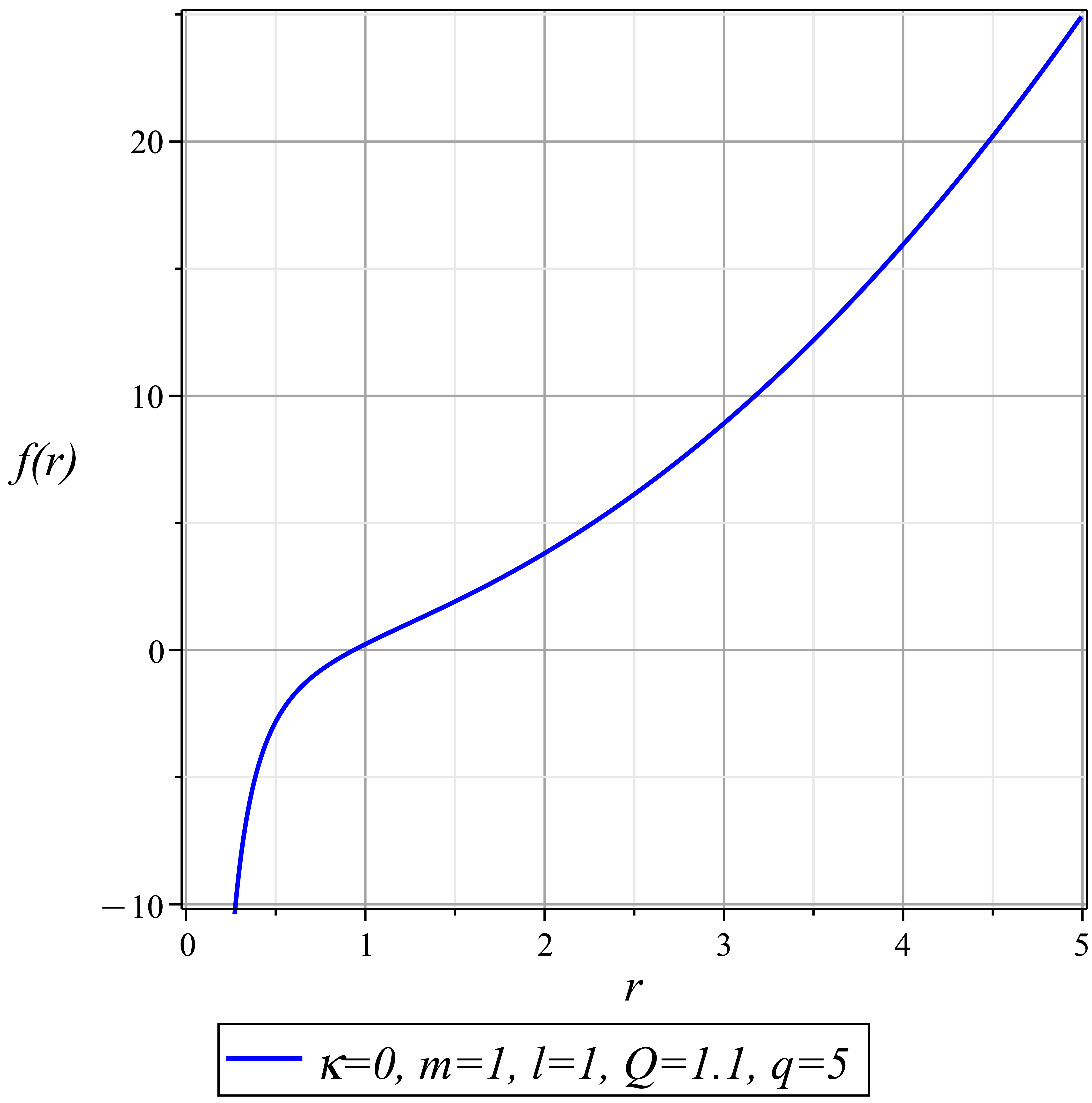
Figure 1: An approximated behavior of $f(r)$ for the values $Q=1.1,l=1,\kappa=0,q=5$ and $m=1$. For these values the the behavior of $f(r)$ is more reliable for $r>0.6665$.

Figure (2) shows the approximated behavior of temperature versus horizon which has been illustrated for the parameter values $Q=1.1,l=1,q=5$ and $m=1$.

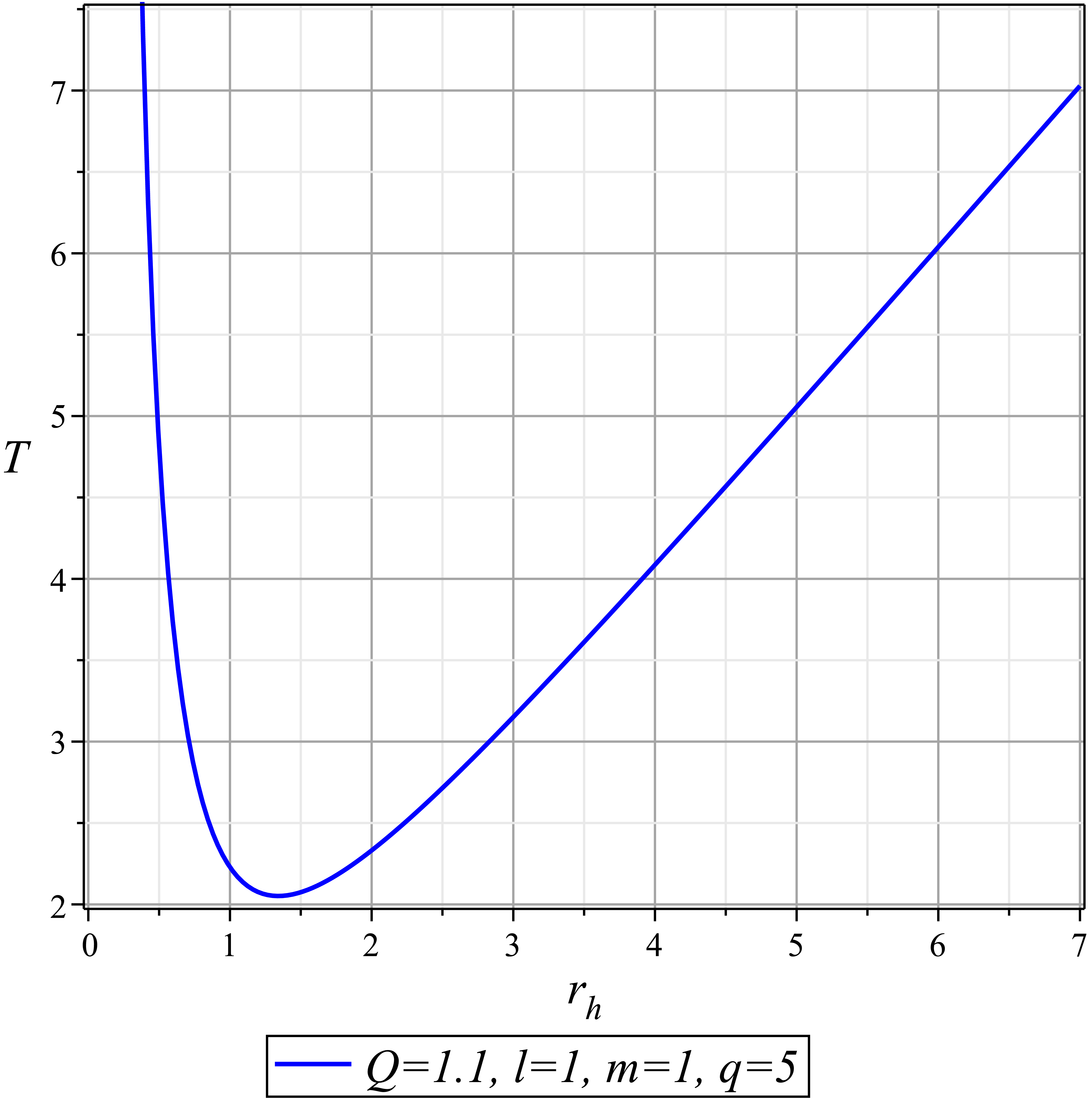
Figure 2: An approximated behavior of temperature for the values $Q=1.1,l=1,q=5$ and $m=1$. It is obvious that a minimum value for the temperature can be seen in this theory.

3 Transport Coefficients

According to the AdS/CFT duality, the field $\phi$ in the bulk corresponds to the operator $\mathcal{O}$ on the boundary of the AdS space. Also, the partition function on the gravity side is equivalent to the partition function on the boundary side,

$$Z_{\text{CFT}}=Z_{\text{string}},$$ (32)

which is realized by GKP–Witten relation[47],[48],[42] as bellow,

$$\bigg{<}\text{exp}{\int_{{\mathbb{S}}^{3}}\phi_{0}\mathcal{O}}\bigg{>}_{CFT}=\text{exp}\big{(}-I_{s}(\phi)\big{)},$$ (33)

Here, $\phi_{0}$ is the value of field on the boundary of AdS and it acts as an external source of a boundary operator $\mathcal{O}$. We set $\phi=A_{\mu}$ and $\mathcal{O}=J^{\mu}$ in the Eq.(33) to calculate DC conductivity. Therefore, we perturb the gauge field as $A_{\mu}\to A_{\mu}+\tilde{A}_{\mu}$ where the perturbation part of gauge field is chosen as $\tilde{A}_{x}=\tilde{A}_{x}(r)e^{-i\omega t}$ [34]. Since, we are in the fluid-gravity duality, it forces us to assume that $\omega$ has small value. By substituting the perturbed part of the gauge field into action (6) and keeping terms up to the second order of $\tilde{A}$, we will have

$$S^{(2)} =\int d^{4}x\frac{e^{\frac{h^{\prime 2}}{q^{2}}}}{f}\left[-f^{2}\left((\partial_{r}\tilde{A}_{x}^{(1)})^{2}+(\partial_{r}\tilde{A}_{x}^{(2)})^{2}+(\partial_{r}\tilde{A}_{x}^{(3)})^{2}\right)\right.$$

$$\left.-\Big{(}(\tilde{A}_{x}^{(1)})^{2}+(\tilde{A}_{x}^{(2)})^{2}\Big{)}(\omega^{2}+h^{2})+(\tilde{A}_{x}^{(3)})^{2}\omega^{2}\right].$$ (34)

By variation of the action $S^{(2)}$ with respect to $\tilde{A}_{x}^{a}$ we have,

$$q^{2}f\left(f\tilde{A}_{x}^{(1)^{\prime}}\right)^{\prime}+q^{2}(\omega^{2}+h^{2})\tilde{A}_{x}^{(1)}+f^{2}\tilde{A}_{x}^{(1)^{\prime}}h^{\prime}h^{\prime\prime}=0,$$ (35)

$$q^{2}f\left(f\tilde{A}_{x}^{(2)^{\prime}}\right)^{\prime}+q^{2}(\omega^{2}+h^{2})\tilde{A}_{x}^{(2)}+f^{2}\tilde{A}_{x}^{(2)^{\prime}}h^{\prime}h^{\prime\prime}=0,$$ (36)

and

$$q^{2}f\left(f\tilde{A}_{x}^{(3)^{\prime}}\right)^{\prime}+q^{2}\omega^{2}\tilde{A}_{x}^{(3)}+2f^{2}h^{\prime}h^{\prime\prime}\tilde{A}_{x}^{(3)^{\prime}}=0.$$ (37)

First, we solve Eq.(35), Eq.(36) and Eq.(37) near the event horizon. We consider the solutions of $\tilde{A}_{x}^{(a)}$ as follows,

$$\tilde{A}_{x}^{(a)}\sim(r-r_{h})^{z_{a}}\,,\qquad a=1,2,3\,\,\,\,,$$ (38)

where,

$$z_{1} =z_{2}=\pm i\frac{\sqrt{\omega^{2}+h(r_{h})^{2}}}{4\pi T},$$ (39)

$$z_{3} =\pm i\frac{\omega}{4\pi T}.$$ (40)

To solve Eq.(35), Eq.(36) and Eq.(37), we use following ansatzs,

$$\tilde{A}_{x}^{(1)}=\tilde{A}^{(1)}_{\infty}\Big{(}\frac{-3f}{\Lambda r^{2}}\Big{)}^{z_{1}}\Big{(}1+i\omega h_{1}(r)+\cdots\Big{)},$$ (41)

$$\tilde{A}_{x}^{(2)}=\tilde{A}^{(2)}_{\infty}\Big{(}\frac{-3f}{\Lambda r^{2}}\Big{)}^{z_{2}}\Big{(}1+i\omega h_{2}(r)+\cdots\Big{)},$$ (42)

and

$$\tilde{A}_{x}^{(3)}=\tilde{A}^{(3)}_{\infty}\Big{(}\frac{-3f}{\Lambda r^{2}}\Big{)}^{z_{3}}\Big{(}1+i\omega h_{3}(r)+\cdots\Big{)},$$ (43)

where $\tilde{A}^{(a)}_{\infty}$ is the value of fields on the boundary and $z_{i}$’s are the minus branch of (39) and (40).
By substituting Eq. (41) into Eq.(35) and keeping up to the first order of $\omega$, we obtain,

$$i\pi^{2}q^{2}r^{2}T^{2}h(r_{h})^{2}h_{1}((r)f^{\prime}(r)^{2}-16iq^{2}r^{2}h(r)^{2}h_{1}(r)-$$

$$4rf\left(\pi Th_{r_{h}}h_{1}(r)\left(q^{2}rf^{\prime\prime}-2f^{\prime}\left(q^{2}-rh^{\prime}h^{\prime\prime}\right)\right)+2q^{2}rf^{\prime}-\left(\pi Th(r_{h})+2i\right)h_{1}^{\prime}+i\pi^{2}q^{2}T^{2}h(r_{h})^{2}h_{1}f^{\prime}\right)-$$

$$4f^{2}\left(4ir\left(q^{2}rh_{1}^{\prime\prime}+h_{1}^{\prime}\left(2rh^{\prime}h^{\prime\prime}+i\pi q^{2}Th(r_{h})\right)\right)+2\pi Th(r_{h})h_{1}\left(q^{2}-2rh^{\prime}h^{\prime\prime}\right)-i\pi^{2}q^{2}T^{2}h(r_{h})^{2}h_{1}\right)=0.$$ (44)

The equation for $h_{2}(r)$ is the same as $h_{1}(r)$.
By substituting Eq.(43) into Eq.(37) and considering the first order of $\omega$, we obtain,

$$r\left(f^{\prime}\left(-2rh^{\prime}h^{\prime\prime}+q^{2}\left(rh_{3}^{\prime}-2\right)\right)+q^{2}rf^{\prime\prime}\right)+f\left(-2rh^{\prime}h^{\prime\prime}\left(rh_{3}^{\prime}-2\right)+q^{2}\left(r^{2}h_{3}^{\prime\prime}+2\right)\right)=0.$$ (45)

The solution for $h_{3}(r)$ is as bellow,

$$h_{3}(r)=C_{3}+\int_{1}^{r}\Bigg{(}\frac{2}{u}+\frac{C_{4}e^{\frac{h^{\prime}(u)^{2}}{q^{2}}}-f^{\prime}(u)}{f(u)}\Bigg{)}du,$$ (46)

where $C_{3}$ and $C_{4}$ are integration constants. The near horizon behavior of $h_{3}(r)$ is,

$$h_{3}\approx\bigg{(}\frac{C_{4}e^{-\frac{h^{\prime}(r)^{2}}{q^{2}}}-4\pi T}{4\pi T}\bigg{)}\log(r-r_{h})+\text{finite terms}.$$ (47)

$C_{4}$ can be determined by demanding regularity of $h_{3}(r)$ at event horizon. In other words,

$$C_{4}=4\pi T{e^{\frac{h^{\prime}(r)^{2}}{q^{2}}}}.$$ (48)

By substituting the solution of $\tilde{A}_{x}^{(3)}$ into Eq.(3) and variation with respect to $\tilde{A}^{(3)}_{\infty}$ , Green’s function can be read as,

$$G_{xx}^{(33)}(\omega,\vec{0})=(\tilde{A}_{x}^{(3)})^{*}f(r)\partial_{r}\tilde{A}_{x}^{(3)}\bigg{|}_{r\to\infty}=i\omega C_{4}.$$ (49)

By using Kubo formula, $\sigma^{(ab)}_{ij}(k_{\mu})=-\mathop{\lim}\limits_{\omega\to 0}\frac{1}{\omega}\Im G^{(ab)}_{ij}(k_{\mu})$, we have:

$$\sigma_{xx}^{(33)}=-\mathop{\lim}\limits_{\omega\to 0}\frac{1}{\omega}\Im G^{ij}(k_{\mu})=e^{\frac{h^{\prime}(r_{h})^{2}}{q^{2}}}=e^{W[\frac{4e^{\frac{2C_{1}}{q^{2}}}}{q^{2}r_{h}^{4}}]}.$$ (50)

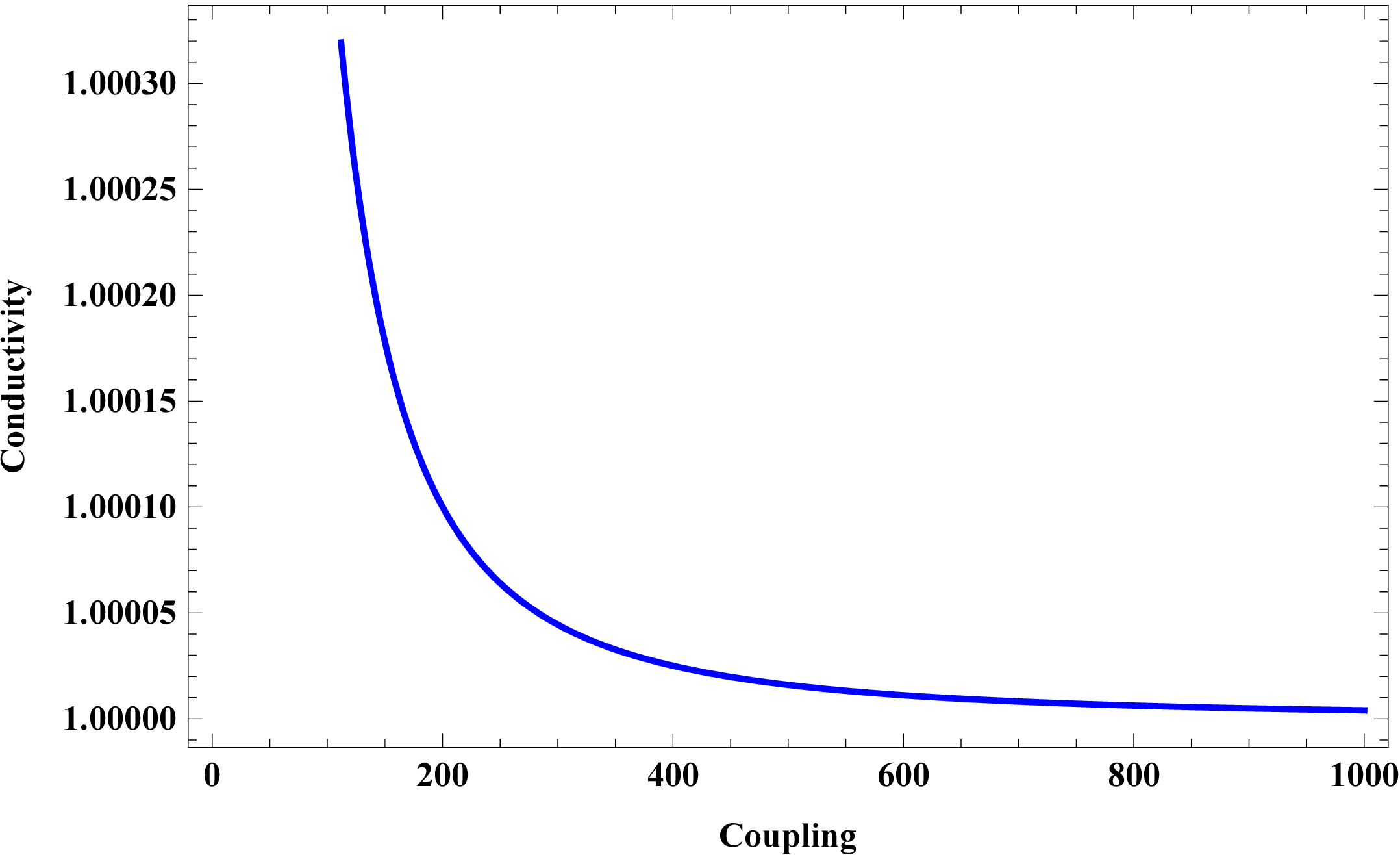
Figure 3: $\sigma_{xx}^{(33)}-q$ diagram for $r_{h}=1$.

The conductivity bound is preserved for $e^{W[\frac{4e^{\frac{2C_{1}}{q^{2}}}}{q^{2}r_{h}^{4}}]}>1$ and it is violated for
$0<e^{W[\frac{4e^{\frac{2C_{1}}{q^{2}}}}{q^{2}r_{h}^{4}}]}<1$.

In the limit of $q\to\infty$ we have non-abelian Yang-Mills theory and the conductivity bound is saturated.

$$\sigma_{xx}^{(33)}=1.$$ (51)

The value of $\sigma_{xx}^{(11)}$ and $\sigma_{xx}^{(22)}$ is calculated by the same procedure of $\sigma_{xx}^{(33)}$ which results in,

$$\sigma_{xx}^{(11)}=\sigma_{xx}^{(22)}=0.$$ (52)

It means that the color non-abelian DC conductivity in terms of color indices is diagonal and also Ohm’s law is diagonal in this model. If we consider the gauge field (12) in $\sigma_{1}$ or $\sigma_{2}$ directions, conductivity will be non-zero in these directions.
The ratio of shear viscosity to entropy density is as follows,

$$\frac{\eta}{s}=\frac{1}{4\pi}\phi(r_{h})^{2},$$ (53)

where $\phi$ is the perturbed part of the metric[44].
Therefore, we perturb the metric as $g_{\mu\nu}\to g_{\mu\nu}+\frac{r^{2}}{l^{2}}\phi(r)$ and substitute into the action (6). Then, we expand the action up to the second order of $\phi$. Finally, the equation of motion of $\phi(r)$ is given by varying the resulted action with respect to $\phi(r)$ which leads to,

$$\phi^{\prime}f^{\prime}+f\phi^{\prime\prime}=0.$$ (54)

The solution of the $\phi(r)$ is as follows,

$$\phi(r)=C_{5}+C_{6}\int^{r}\frac{1}{f(u)}du.$$ (55)

We consider the solution of $\phi(r)$ near the event horizon as,

$$\phi(r)=C_{5}+\frac{C_{6}}{4\pi T}\log(r-r_{h}).$$ (56)

By demanding the regularity of $\phi(r)$ on the event horizon. We have,

$$C_{6}=0.$$ (57)

By applying the normalization condition on Eq.(55), we have $C_{5}=1$. So,

$$\phi(r)=1.$$ (58)

Finally, the ratio of shear viscosity to entropy density is given by,

$$\frac{\eta}{s}=\frac{1}{4\pi}\phi(r_{h})^{2}=\frac{1}{4\pi}.$$ (59)

The ratio $\frac{\eta}{s}$ is satisfied for Einstein-Hilbert gravity as the universal relation $\frac{\eta}{s}\geq\frac{1}{4\pi}$. This bound which is called KSS bound [56] can be violated for higher derivative gravitational theories [5, 6] while, it is saturated for Einstein-Hilbert gravity[26].
Our result shows that the KSS bound is saturated for nonlinear exponential Yang-Mills AdS black brane.

4 Conclusion

We introduced non-abelian exponential Einstein Yang-Mills AdS black brane solution and calculated the non-abelian color DC conductivity and the ratio of shear viscosity to entropy density for this model. There is a conjecture that conductivity is bounded by the universal value $\sigma\geq 1$. Our result shows that the conductivity bound is violated for $0<e^{\frac{h^{\prime}(r_{h})^{2}}{q^{2}}}<1$ and it is preserved for $e^{\frac{h^{\prime}(r_{h})^{2}}{q^{2}}}\geq 1$ in non-abelian exponential gauge theory but this bound is saturated for Yang-Mills theory[57]. The conductivity bound can be violated for a nonlinear model like the exponential model and the violation of conductivity bound is related to Mott insulators.
The ratio of shear viscosity to entropy density in this model, $\frac{\eta}{s}=\frac{1}{4\pi}$, is the same as this value for Einstein-Hilbert gravity. It means that the coupling of the field theory dual to our model is the same as the coupling of the field theory dual to the Einstein AdS black brane solution, but the color conductivity is different. We note that $\frac{\eta}{s}$ is proportional to the inverse of the square of the field theory coupling i.e. $\frac{\eta}{s}\sim\frac{1}{\lambda^{2}}$.

Acknowledgment We would like to thank Ahmad Moradpouri for useful comments and suggestions.

Data Availability statement

All data that support the findings of this study are included within the article (and any supplementary files).

References

• [1] D. H. Delphenich, [arXiv:hep-th/0309108 [hep-th]].
• [2] D. H. Delphenich, [arXiv:hep-th/0610088 [hep-th]].
• [3] B. Eslam Panah, [arXiv:2103.08343 [physics.class-ph]].
• [4] M. Sadeghi and S. Parvizi, [arXiv:1411.2358 [hep-th]].
• [5] M. Sadeghi and S. Parvizi, Class. Quant. Grav. 33, no.3, 035005 (2016) doi:10.1088/0264-9381/33/3/035005 [arXiv:1507.07183 [hep-th]].
• [6] S. Parvizi and M. Sadeghi, Eur. Phys. J. C 79, no.2, 113 (2019) doi:10.1140/epjc/s10052-019-6631-9 [arXiv:1704.00441 [hep-th]].
• [7] C. S. Camara, M. R. de Garcia Maia, J. C. Carvalho and J. A. S. Lima, Phys. Rev. D 69, 123504 (2004) [arXiv:astro-ph/0402311 [astro-ph]].
• [8] D. N. Vollick, Phys. Rev. D 78, 063524 (2008) [arXiv:0807.0448 [gr-qc]].
• [9] A. E. Shabad and V. V. Usov, Phys. Rev. D 83, 105006 (2011) [arXiv:1101.2343 [hep-th]].
• [10] R. Garcia-Salcedo, T. Gonzalez and I. Quiros, Phys. Rev. D 89, no.8, 084047 (2014) [arXiv:1312.3163 [gr-qc]].
• [11] P. Gaete and J. Helayël-Neto, Eur. Phys. J. C 74, no.3, 2816 (2014) [arXiv:1312.5157 [hep-th]].
• [12] M. Dehghani, Eur. Phys. J. Plus 134, no.9, 426 (2019)
• [13] M. Sadeghi, doi:10.1139/cjp-2023-0150 [arXiv:2203.05023 [hep-th]].
• [14] S. I. Kruglov, Ann. Phys. (Berlin) 527, 397 (2015) [arXiv:1410.7633].
• [15] M. Sadeghi and S. M. M. Khansari, doi:10.1007/s12648-023-02926-2 [arXiv:2308.08817 [hep-th]].
• [16] M. Born, and L. Infeld, Proc. Roy. Soc. (Lond.) A144 (1934) 425.
• [17] M. Born, Ann. Inst. Poincar´e 7 (1939) 155.
• [18] Z. Bialynicka-Birula, and I. Bialynicka-Birula, Phys. Rev. D 2 (1970) 2341.
• [19] H. J. Mosquera, and J. M. Cuesta Salim, Astrophys. J. 608 (2004) 925.
• [20] C. Corda and H. J. Mosquera Cuesta, Mod. Phys. Lett. A 25, 2423-2429 (2010) [arXiv:0905.3298 [gr-qc]].
• [21] E. Ayon-Beato and A. Garcia, Gen. Rel. Grav. 31, 629-633 (1999) [arXiv:gr-qc/9911084 [gr-qc]].
• [22] S. H. Hendi, Annals Phys. 333, 282-289 (2013) doi:10.1016/j.aop.2013.03.008 [arXiv:1405.5359 [gr-qc]]
• [23] S. H. Hendi, JHEP 03, 065 (2012) doi:10.1007/JHEP03(2012)065 [arXiv:1405.4941 [hep-th]].
• [24] M. Sadeghi, Indian J. Phys. 96, no.14, 4341-4345 (2022) [arXiv:2111.12916 [hep-th]].
• [25] D.T. Son, Nuclear Physics B (Proc. Suppl.) 192–193 (2009) 113–118.
• [26] G. Policastro, D. T. Son and A. O. Starinets, Phys. Rev. Lett.  87, 081601 (2001) [hep-th/0104066].
• [27] P. Kovtun, J. Phys. A 45 (2012) 473001[arXiv:1205.5040 [hep-th]].
• [28] S. Bhattacharyya, V. E. Hubeny, S. Minwalla and M. Rangamani, JHEP 0802, 045 (2008) [arXiv:0712.2456 [hep-th]].
• [29] M. Rangamani, Class. Quant. Grav.  26, 224003 (2009) [arXiv:0905.4352 [hep-th]].
• [30] J. Bhattacharya, S. Bhattacharyya, S. Minwalla and A. Yarom, JHEP 1405, 147 (2014) [arXiv:1105.3733 [hep-th]].
• [31] J. M. Maldacena, Adv. Theor. Math. Phys. 2 (1998), 231-252 [arXiv:hep-th/9711200 [hep-th]].
• [32] K. Ziegler, Phys. Rev. B, 75, (2007).
• [33] M. Baggioli and O. Pujolas, JHEP 01 (2017), 040 [arXiv:1601.07897 [hep-th]].
• [34] M. Baggioli and O. Pujolas, JHEP 12 (2016), 107 doi:10.1007/JHEP12(2016)107 [arXiv:1604.08915 [hep-th]].
• [35] P. Kovtun, D. T. Son and A. O. Starinets, Phys. Rev. Lett. 94 (2005), 111601 [arXiv:hep-th/0405231 [hep-th]].
• [36] X. H. Feng, H. S. Liu, H. Lü and C. N. Pope, JHEP 11 (2015), 176 doi:10.1007/JHEP11(2015)176 [arXiv:1509.07142 [hep-th]].
• [37] M. Sadeghi, Mod. Phys. Lett. A 36 (2021) no.28, 2150202 doi:10.1142/S0217732321502023 [arXiv:2007.09688 [hep-th]]
• [38] M. Bravo-Gaete and F. F. Santos, Eur. Phys. J. C 82, no.2, 101 (2022) doi:10.1140/epjc/s10052-022-10064-y [arXiv:2010.10942 [hep-th]].
• [39] M. Bravo-Gaete and M. M. Stetsko, Phys. Rev. D 105, no.2, 024038 (2022) doi:10.1103/PhysRevD.105.024038 [arXiv:2111.10925 [hep-th]].
• [40] M. Bravo-Gaete, F. F. Santos and H. Boschi-Filho, Phys. Rev. D 106, no.6, 066010 (2022) doi:10.1103/PhysRevD.106.066010 [arXiv:2201.07961 [hep-th]].
• [41] K. A. Mamo, JHEP 10, 070 (2012) doi:10.1007/JHEP10(2012)070 [arXiv:1205.1797 [hep-th]].
• [42] A. J. Ferreira-Martins, P. Meert and R. da Rocha, Eur. Phys. J. C 79, no.8, 646 (2019) doi:10.1140/epjc/s10052-019-7167-8 [arXiv:1904.01093 [hep-th]].
• [43] A. J. Ferreira–Martins, P. Meert and R. da Rocha, Nucl. Phys. B 957, 115087 (2020) doi:10.1016/j.nuclphysb.2020.115087 [arXiv:1912.04837 [hep-th]].
• [44] S. A. Hartnoll, D. M. Ramirez and J. E. Santos, JHEP 03, 170 (2016) doi:10.1007/JHEP03(2016)170 [arXiv:1601.02757 [hep-th]].
• [45] B. L. Shepherd and E. Winstanley, Phys. Rev. D 93, no. 6, 064064 (2016) doi:10.1103/PhysRevD.93.064064 [arXiv:1512.03010 [gr-qc]].
• [46] A. Dey, S. Mahapatra and T. Sarkar, JHEP 01, 088 (2016) doi:10.1007/JHEP01(2016)088 [arXiv:1510.00232 [hep-th]].
• [47] E. Witten, Adv. Theor. Math. Phys. 2, 253-291 (1998) doi:10.4310/ATMP.1998.v2.n2.a2 [arXiv:hep-th/9802150 [hep-th]].
• [48] S. S. Gubser, I. R. Klebanov and A. M. Polyakov, Phys. Lett. B 428, 105-114 (1998) doi:10.1016/S0370-2693(98)00377-3 [arXiv:hep-th/9802109 [hep-th]].
• [49] X. H. Ge, Y. Matsuo, F. W. Shu, S. J. Sin and T. Tsukioka, JHEP 10, 009 (2008) doi:10.1088/1126-6708/2008/10/009 [arXiv:0808.2354 [hep-th]].
• [50] D. F. Litim and C. Manuel, Nucl. Phys. B 562, 237-274 (1999) doi:10.1016/S0550-3213(99)00531-3 [arXiv:hep-ph/9906210 [hep-ph]].
• [51] S. I. Kruglov, Eur. Phys. J. C 75, no.2, 88 (2015) doi:10.1140/epjc/s10052-015-3314-z [arXiv:1411.7741 [hep-th]].
• [52] S. Gangopadhyay and D. Roychowdhury, JHEP 05, 002 (2012) doi:10.1007/JHEP05(2012)002 [arXiv:1201.6520 [hep-th]].
• [53] A. Donos and J. P. Gauntlett, JHEP 1411, 081 (2014) [arXiv:1406.4742 [hep-th]].
• [54] X. H. Ge, Y. Matsuo, F. W. Shu, S. J. Sin and T. Tsukioka, JHEP 10, 009 (2008) [arXiv:0808.2354 [hep-th]].
• [55] X. H. Ge and S. J. Sin, Eur. Phys. J. C 80, no.8, 695 (2020) doi:10.1140/epjc/s10052-020-8288-9 [arXiv:2004.12191 [hep-th]].
• [56] G. Policastro, D. T. Son and A. O. Starinets, JHEP 09, 043 (2002) doi:10.1088/1126-6708/2002/09/043 [arXiv:hep-th/0205052 [hep-th]].
• [57] S. Parvizi; M. Sadeghi. Iranian Journal of Physics Research, 20, 1, 2020, 139-145. doi: 10.47176/ijpr.20.1.39001.