Lindbladian approach to theory
Abstract
The theory describes inelastic tunneling of particles through junctions integrated into an electric circuit. The inelasticity stems from the interaction between the photonic field of the circuit and the tunneling particles possessing electric charge. In the conventional approach to the theory, the tunneling rate and the electric current through the junction are derived using Fermi’s golden rule. The derivation is carried out to leading order in the tunnel coupling between the leads and includes an averaging over the environmental photonic degrees of freedom. Tracing out the environmental degrees of freedom is also commonly used for open quantum systems when deriving dynamical equations such as the Lindbladian. In this work, we reveal the relations between the theory and the Lindbladian dynamics. We demonstrate that the assumptions of the Fermi’s golden rule are essentially equivalent with the Born-Markovian approximation used in the Lindbladian formalism. The resulting quantum master equation enables us to obtain not only the electric current but various other quantities, including for instance the heat current parametrized by the same function, in a systematic and convenient way.
I Introduction
Tunneling is one of the most peculiar quantum phenomena. In contrast to classical behavior, quantum transmission is also possible through potential barriers exceeding the total energy of the particle. Quantum tunneling has attracted much interest due to the wide range of applications including superconducting quantum interference devices [1, 2], scanning tunneling microscopy [3, 4, 5, 6, 7], atomic scale devices [8, 9, 10], quantum dots [11, 12, 13] and resonant tunneling diodes [14, 15].
In most situations, the tunneling event can be considered a closed (i.e., unitary) process in the sense that the particle does not interact with the environment. In some experiments [16, 17, 6, 18, 19], however, the coupling to the electromagnetic environment significantly influences the transport properties. The electromagnetic field arises from the electric circuit into which the junction is embedded and typically plays an important role in junctions with low capacity (large charging energy). The effects of the coupling between a tunneling particle and the quantized electromagnetic (photonic) bath is conventionally described by the theory [20, 21, 22, 23, 24]. The theory is based on Fermi’s golden rule describing the transmission probability rate between an initial and a final state with equal energies. By taking into account the energy of both the tunneling particles and the photons, and by averaging over the photonic degrees of freedom, one can derive an analytical expression for the characteristics. The key quantity appearing in the formula is the function which describes the probability that the tunneling particle emits a photon of energy to the environment.
Another very commonly used technique to describe the system-bath interaction is the Lindbladian formalism [25, 26, 27, 28, 29] which appears quite different in form and spirit: while the theory describes inelastic tunneling of particles, the more general Lindbladian equation describes the dynamics of open quantum systems. The relation between the theory and the Lindbladian dynamics has not been discussed so far. In this paper, we present the Lindbladian approach by applying the Born-Markovian approximation and by integrating out the photonic degrees of freedom. We also demonstrate how the resulting Lindblad equation can be used to calculate physical observables. We emphasize that the Lindbladian approach does not supersede the approach; the aim of the present work is rather to create a link between the two theoretical fields. In particular, we compare the assumptions of the conventional Fermi’s golden rule and the Lindbladian approach. We show that the approximations of the two approaches are essentially the same. We believe, however, that the Lindbladian approach has one significant technical advantage: it provides a convenient framework for calculating various quantities beyond the characteristics.
The paper is structured as follows. After defining the problem in Sec. II, in Sec. III we review the main steps of the conventional approach by focusing on the approximations implied in the Fermi’s golden rule. These approximations are compared to the assumptions made during the derivation of the Lindbladian equation in Sec. IV. In Secs. V and VI, the electric and heat current are calculated using the Lindbladian framework.
II Problem statement
The system of interest is the tunnel junction between two leads as shown in Fig. 1. The Hamiltonian of the system is given by
| (1) |
Here
| (2) |
describes the electrons of the left () and the right () leads, and are the annihilation operators of electrons with wavenumber and spin . The energy spectra and will be kept general for most of the calculation.

The leads are coupled to a thermal bath with temperature and particle reservoirs setting the chemical potentials to and , such that with the charge of the electron and the bias voltage applied in the electric circuit.
The tunneling through the junction is described by
| (3) |
where is a charge counting operator acting on the photonic field. From the circuit point of view, the junction is a capacitor. The operator shifts the charge on the capacitor by the unit charge . The tunneling amplitudes include the factor of where and designate the number of momentum modes in the left and right lead, respectively.
The term describes the electromagnetic field of the circuit which depends on the actual circuit in which the junction is embedded. In the forthcoming discussion, it is assumed that the environment is in thermal equilibrium with the same temperature as the thermal bath of the leads.
III Fermi’s golden rule approach
We briefly revisit the conventional derivation of the theory for a single junction [20]. We will particularly focus on the approximations made in the derivation. These will later be compared to those of the Lindbladian approach.
The approach is based upon Fermi’s golden rule which is used to calculate the transmission rate. The transmission from the left lead state with energy to the right lead state with energy is characterized by the rate of
| (4) | |||||
where denotes the state of the photonic bath with energy and is the Dirac delta. It is important to note that Fermi’s golden rule is obtained from the first-order perturbation theory and is valid if the tunneling is weak. To be more precise, the transition probability from the left lead state to the right lead state is obtained as where is the time evolved state with the initial condition of . In the matrix element , we keep only first order terms in the tunneling amplitude.
The derivation of Fermi’s golden rule includes an infinite-time limit of the average transmission probability, . This infinite time limit results in the decay of all transition probabilities between the initial and the final states with a finite energy difference. By using the infinite time limit, it is also assumed implicitly that the tunneling events are independent and that there is no temporal overlap between any two events.
The overall transition rate from left to right is obtained as a sum of the products of the elementary transition probabilities and occupation probabilities as described in Ref. [20]. It is assumed that the coupling between the photonic environment and the electron does not significantly affect the state of the environment. In reality, of course, the state of the environment is modified by the coupling but since the transition probabilities are already in second order in the tunneling these modifications result only in higher order corrections. For the same reason, the leads can also be assumed to remain in thermal equilibrium with the temperature and chemical potentials and .
By taking advantage of the thermal equilibrium, the sum over the environmental degrees of freedom can be performed leading to the tunneling rate
| (5) |
where we use the shorthand notation and where is the Fermi function and is the inverse temperature. The function is defined as
| (6) |
with the thermal equilibrium density operator of the photonic bath. The function is related to the charge relaxation through the electric circuit and can be computed from the properties of the particular circuit [20]. From the electron point of view, the function represents the probability that the tunneling electron emits a photon with an energy to the environment (for ) or absorb it (for ).
Similarly to Eq. (5), the total tunneling rate from right to left can also be obtained and the electric current is finally calculated as .
We note that the derivation presented here differs from that of Ref. [20] in a canonical transformation and in that the bias voltage appears as the difference of the chemical potential in the two leads. The final result is the same. Our choice of presentation enables easier comparison between the Fermi golden rule and the Lindbladian approaches.
IV Lindbladian approach
In this section, we present an alternative theoretical description of the coupling between the tunneling electrons and the electromagnetic field of the circuit. We consider the latter as an energy reservoir for the electrons and follow the standard procedure of the microscopic derivation of the Lindblad equation [27]. The goal of this section is to demonstrate that the approximations of the Fermi’s golden rule are essentially equivalent to the Born-Markovian approximation used for the Lindblad equation.
In the standard procedure[27], the time evolution is described within the interaction picture with being the unperturbed Hamiltonian. The von Neumann equation can be reformulated as
| (7) |
where is the density matrix of the whole system including both the electronic and photonic degrees of freedom. Square brackets denote the usual commutators and stands for the initial density matrix. denotes the tunneling Hamiltonian in the interaction picture.
To reduce the Hilbert space to the electronic degrees of freedom, we trace out the environmental degrees of freedom on both sides of the equation. The partial trace leads to describing solely the electronic degrees of freedom. For the initial condition, we assume that . In our specific case of a single junction, this assumption traces back to which holds true if describes the thermal equilibrium state of the bath.
Furthermore, it is also assumed that the coupling between the system and the environment is weak, and that the system affects the state of the reservoir only negligibly. Hence, on the right-hand side of the equation, which is already second order in the coupling, we can assume that , where is the bath density operator in thermal equilibrium with the temperature . Similarly to the Fermi’s golden rule approach, the effects of the coupling on the bath would result in higher order corrections only. This assumption is called Born approximation.
In the standard procedure, the next assumption is that the environment relaxes much faster than the typical timescales of the system evolution. This Markovian approximation can also be rephrased as a statement that the time evolution of the system has no memory effects. Technically, the time argument of the density matrix is replaced by indicating that the system density matrix does not change essentially while the bath relaxes. In addition to this change of argument, we also set the lower limit of the integration in Eq. (7) to in accordance with the idea that no memory effects from the initial state are kept. The physical meaning of the Markovian assumption is that after a tunneling event (also referred to as a jump process in the Lindbladian language) the bath achieves complete relaxation before another event occurs. This is essentially the same assumption as the infinite-time limit applied in the Fermi’s golden rule approach.
The standard form of the resulting equation is usually achieved by changing the integral variable from to leading to
| (8) | |||||
Now, we substitute into this equation the tunneling Hamiltonian which is given by
| (9) |
in the interaction picture. Here, we have defined the process operators as
| description | frequency | |
|---|---|---|
| () | ||
| () |
where we have also introduced the composite process index . The operator describes a tunneling process between a left lead state with momentum and a right lead state with momentum , spin and is the direction of the tunneling. If the tunneling process occurs from left to right, , and for the opposite direction. In the exponent of Eq. (9), indicates the direction of the process . In the following, we will use and instead of and for the sake of brevity.
After substituting into Eq. (8) and carrying out the integration over , we obtain
| (10) | |||||
where the bath correlation function has been defined as
| (11) |
In the standard derivation, the exponential factors are assumed to describe very fast oscillations. By applying the rotating wave approximation, we neglect terms where the processes and have different frequencies and keep only terms with . In some situations, this approximation does not hold true and one has to handle the nonsecular Lindblad equation with time-dependent coefficients [30, 31]. In the case of tunneling through the single junction, the terms with do not contribute to the electric current nor to the heat current, hence they would play no role even if retained.
By applying the rotating wave approximation and returning to the Schrödinger picture representation, we obtain
| (12) |
which is the Lindblad equation for the tunneling electrons. In this equation, denotes anti-commutation. We have also defined
| (13) |
which, apart from a factor of , is the same as the function from Eq. (6) if , with . Furthermore, we defined the Lamb shift Hamiltonian as
| (14) |
So far, we have derived the Lindblad equation for the tunneling particles which is the full dynamical equation for the density matrix. Based on the density matrix, one can compute various observables, not only the electric current but also, for example, the dissipated heat loss. We note that these quantities could possibly be computed using the conventional approach as well but we believe that the Lindbladian approach provides a more convenient and systematic way.
Further advantage of the Lindbladian is that it provides a platform to add further effects to the model and also to describe slowly varying transient phenomena such us switching on the bias voltage. Furthermore, the wide range of numerical tools developed for solving Lindblad master equations can be applied [32].
V Electric current
In this section, we calculate the current flowing through the junction based on the Lindblad equation (12). Since the Lindbladian contains only particle operators, the current must also be expressed in terms of particle operators rather than circuit variables. We start with the expectation value of
| (15) |
where
| (16) |
is the operator for the total charge in the left lead. The expectation value of the current flowing from left to right is calculated as
| (17) |
We substitute the right-hand side of the Lindblad equation into , make use of the cyclic properties of the trace and the relation . We obtain
| (18) |
Due to , the current is already in the order of in the tunneling amplitude which is the leading order within the Born approximation. Therefore, we can assume that in the steady state the leads achieve thermal equilibrium, . We note that this steady state is not reached by the dissipation described by the jump processes in Eq. (12). In reality, the leads are coupled to other reservoirs: phonons act as a heat bath and wires act as charge reservoirs. The effects of these are expected to be much stronger than the dissipation generated by the tunneling. They thus drive the leads to the thermal equilibrium state with a well-defined temperature and chemical potential.
In thermal equilibrium, and . Deviations from these values occur only in higher orders in . When evaluating the trace in Eq. (18), terms like must be calculated. Due to the thermal equilibrium, only the terms contribute and we obtain
| (19) |
which is the same as the current obtained from the Fermi’s golden rule by evaluating from Eq. (5). The correspondence is established by
| (20) |
which directly connects the jump coefficients of the Lindbladian with the distribution function.
If does not depend on the wavenumber, and the density of states on each lead is also approximated by a constant, or , the current is calculated as
| (21) | |||||
| (22) | |||||
where
| (23) |
is the ohmic resistance of the junction. Eq. (22) is identical to Eq. (51) of Ref. [20].
In this section, we presented the relation between the conventional approach to the theory and the Lindbladian formalism. We have seen that the assumptions of Fermi’s golden rule are essentially equivalent to the Born-Markovian approximation used for the Lindblad equation. Namely, both approaches are valid if the coupling between the system and the bath is weak and the results are given up to leading order only. Furthermore, both approaches assume that the tunneling events are independent from each other and that the reservoir completely relaxes between consecutive events.
VI Dissipated heat
The dissipated heat is a fundamentally important quantity [33]. Furthermore, it can be used to characterize devices through Joule spectrometry, e.g. in hybrid superconducting devices [34]. In this section, we study the heat current flowing through the junction with normal-state leads. The total energy of the left lead is given by the operator and its expectation value is given by
| (24) |
The heat flow from the left lead is computed as
| (25) |
By substituting the right-hand side of the Lindblad equation and taking advantage of , we obtain
| (26) |
where we used again that the leads are in thermal equilibrium. Similar formula can be derived for the heat flow to the right lead.
| (27) |
Without environmental effects, , the two heat currents are the same, . In the presence of the photonic bath, however, some part of the heat current which leaves the left lead does not arrive on the right lead but gets dissipated into the environment. The dissipated heat is calculated as
| (28) |
By considering constant density of states and tunneling amplitude and taking the limits of infinite system size and infinitely large bandwidth, the sum is rewritten as
| (29) |
In the formula, is the electric resistance of the junction as given in Eq. (23). The dissipated heat has been computed numerically for an environment, see Fig. 2. The circuits are distinguished based on the quality factor defined as following Ref. [20]. In each case, has also been set. The quality factor indicates how pronounced are the resonant peaks in the function. For lower values of , the ohmic resistance becomes more dominant.
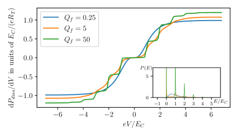
At low bias voltage, the dissipated heat has a rich structure and depends strongly on the specific circuit. At high voltages, however, the dissipated heat behaves as which is noticeably distinct from the quadratic behavior characteristic of ohmic resistances. This result is particularly interesting since the characteristics do exhibit the ohmic behavior in this regime, . It can also be shown that in the large bias voltage limit, the dissipated heat through the junction is given by
| (30) |
where is the average energy emission of a tunneling particle.
We remark that the dissipated heat is not necessarily lost on the ohmic resistance of the electric circuit. It can be shown that even in the case of a simple circuit, the dissipated heat is non-zero. This can be explained by that the photonic environment with a well-defined temperature is coupled to a large heat bath and the dissipated heat can also be lost through this coupling.
VII Conclusion
The theory is the most commonly used approach to explain the transport properties of ultrasmall junctions. In this paper we have revealed the relation between the conventional derivation based on Fermi’s golden rule and the Lindbladian formalism. We emphasize that the Lindbladian approach leads to the same result on the level of characteristics. The Lindbladian approach, however, enables one to include in consideration further effects such as additional dissipative features or tunneling processes without interaction with the photons. Furthermore, the Lindbladian approach also enables the application of the multitude of numerical techniques designed for solving the Lindblad equations to the tunneling phenomena.
One of the main results of the present paper is the demonstration that the infinite-time limit of Fermi’s golden rule and the assumption of the independence of the tunneling events are essentially equivalent to the Markovian approximation applied when deriving the Lindblad equation. We believe that our results extend the conventional theory, open the route to more complex systems, and enable the calculation of more complicated observables. As a demonstration, we have applied the formalism to compute the heat currents through the junction. The dissipated heat exhibits a behaviour at large bias voltage even though the current obeys in this regime.
Acknowledgements.
We acknowledge the support of the Slovenian Research and Innovation Agency (ARIS) under P1-0416 and J1-3008. Á.B. acknowledges the support of the National Research, Development and Innovation Office - NKFIH Project No. K142179.References
- Barone and Paterno [1982] A. Barone and G. Paterno, Physics and applications of the Josephson effect (John Wiley & Sons, 1982).
- Golubov et al. [2004] A. A. Golubov, M. Y. Kupriyanov, and E. Il’ichev, Rev. Mod. Phys. 76, 411 (2004), URL https://link.aps.org/doi/10.1103/RevModPhys.76.411.
- Binnig and Rohrer [1987] G. Binnig and H. Rohrer, Rev. Mod. Phys. 59, 615 (1987), URL https://link.aps.org/doi/10.1103/RevModPhys.59.615.
- Chen [1993] C. J. Chen, Introduction to scanning tunneling microscopy (Oxford University Press, 1993).
- van Houselt and Zandvliet [2010] A. van Houselt and H. J. W. Zandvliet, Rev. Mod. Phys. 82, 1593 (2010), URL https://link.aps.org/doi/10.1103/RevModPhys.82.1593.
- Ast et al. [2016] C. R. Ast, B. Jäck, J. Senkpiel, M. Eltschka, M. Etzkorn, J. Ankerhold, and K. Kern, Nature Communications 7, 13009 (2016), ISSN 2041-1723, URL https://doi.org/10.1038/ncomms13009.
- Karan et al. [2022] S. Karan, H. Huang, C. Padurariu, B. Kubala, A. Theiler, A. M. Black-Schaffer, G. Morrás, A. L. Yeyati, J. C. Cuevas, J. Ankerhold, et al., Nature Physics 18, 893 (2022), ISSN 1745-2481, URL https://doi.org/10.1038/s41567-022-01644-6.
- Agraït et al. [2003] N. Agraït, A. L. Yeyati, and J. M. van Ruitenbeek, Phys. Rep. 377, 81 (2003).
- Bretheau et al. [2011] L. Bretheau, u. Girit, L. Tosi, M. Goffman, P. Joyez, H. Pothier, D. Esteve, and C. Urbina, Comptes Rendus. Physique 13, 89–100 (2011), ISSN 1878-1535, URL http://dx.doi.org/10.1016/j.crhy.2011.12.006.
- Evers et al. [2020] F. Evers, R. Korytár, S. Tewari, and J. M. van Ruitenbeek, Reviews of Modern Physics 92 (2020), ISSN 1539-0756, URL http://dx.doi.org/10.1103/RevModPhys.92.035001.
- Kouwenhoven and Marcus [1998] L. Kouwenhoven and C. Marcus, Physics World 11, 35 (1998).
- van der Wiel et al. [2003] W. G. van der Wiel, S. D. Franceschi, J. M. Elzerman, T. Fujisawa, S. Tarucha, and L. P. Kouwenhoven, Rev. Mod. Phys. 75, 1 (2003).
- Franceschi et al. [2010] S. D. Franceschi, L. Kouwenhoven, C. Schönenberger, and W. Wernsdorfer, Nat. Nanotechnology 5, 703 (2010).
- Esaki and Tsu [1970] L. Esaki and R. Tsu, IBM Journal of Research and Development 14, 61 (1970).
- Sollner et al. [1983] T. C. L. G. Sollner, W. D. Goodhue, P. E. Tannenwald, C. D. Parker, and D. D. Peck, Applied Physics Letters 43, 588–590 (1983), ISSN 1077-3118, URL http://dx.doi.org/10.1063/1.94434.
- Delsing et al. [1989] P. Delsing, K. K. Likharev, L. S. Kuzmin, and T. Claeson, Phys. Rev. Lett. 63, 1180 (1989), URL https://link.aps.org/doi/10.1103/PhysRevLett.63.1180.
- Pekola et al. [2010] J. P. Pekola, V. F. Maisi, S. Kafanov, N. Chekurov, A. Kemppinen, Y. A. Pashkin, O.-P. Saira, M. Möttönen, and J. S. Tsai, Phys. Rev. Lett. 105, 026803 (2010), URL https://link.aps.org/doi/10.1103/PhysRevLett.105.026803.
- Huang et al. [2020] H. Huang, C. Padurariu, J. Senkpiel, R. Drost, A. L. Yeyati, J. C. Cuevas, B. Kubala, J. Ankerhold, K. Kern, and C. R. Ast, Nature Physics 16, 1227 (2020), ISSN 1745-2481, URL https://doi.org/10.1038/s41567-020-0971-0.
- Senkpiel et al. [2020] J. Senkpiel, J. C. Klöckner, M. Etzkorn, S. Dambach, B. Kubala, W. Belzig, A. L. Yeyati, J. C. Cuevas, F. Pauly, J. Ankerhold, et al., Phys. Rev. Lett. 124, 156803 (2020), URL https://link.aps.org/doi/10.1103/PhysRevLett.124.156803.
- Ingold and Nazarov [1992] G.-L. Ingold and Y. V. Nazarov, Charge Tunneling Rates in Ultrasmall Junctions (Springer US, Boston, MA, 1992), pp. 21–107, ISBN 978-1-4757-2166-9, URL https://doi.org/10.1007/978-1-4757-2166-9{_}2.
- Devoret et al. [1990] M. H. Devoret, D. Esteve, H. Grabert, G.-L. Ingold, H. Pothier, and C. Urbina, Phys. Rev. Lett. 64, 1824 (1990), URL https://link.aps.org/doi/10.1103/PhysRevLett.64.1824.
- Girvin et al. [1990] S. M. Girvin, L. I. Glazman, M. Jonson, D. R. Penn, and M. D. Stiles, Phys. Rev. Lett. 64, 3183 (1990), URL https://link.aps.org/doi/10.1103/PhysRevLett.64.3183.
- Martinis et al. [2009] J. M. Martinis, M. Ansmann, and J. Aumentado, Phys. Rev. Lett. 103, 097002 (2009), URL https://link.aps.org/doi/10.1103/PhysRevLett.103.097002.
- Joyez [2013] P. Joyez, Phys. Rev. Lett. 110, 217003 (2013), URL https://link.aps.org/doi/10.1103/PhysRevLett.110.217003.
- Lindblad [1976] G. Lindblad, Communications in Mathematical Physics 48, 119 (1976), ISSN 1432-0916, URL https://doi.org/10.1007/BF01608499.
- Moy et al. [1999] G. M. Moy, J. J. Hope, and C. M. Savage, Phys. Rev. A 59, 667 (1999), URL https://link.aps.org/doi/10.1103/PhysRevA.59.667.
- Breuer and Petruccione [2002] H. Breuer and F. Petruccione, The Theory of Open Quantum Systems (Oxford University Press, 2002), ISBN 9780198520634, URL https://books.google.hu/books?id=0Yx5VzaMYm8C.
- Manzano [2020] D. Manzano, AIP Advances 10, 025106 (2020), ISSN 2158-3226, eprint https://pubs.aip.org/aip/adv/article-pdf/doi/10.1063/1.5115323/12881278/025106_1_online.pdf, URL https://doi.org/10.1063/1.5115323.
- D’Abbruzzo and Rossini [2021] A. D’Abbruzzo and D. Rossini, Phys. Rev. A 103, 052209 (2021), URL https://link.aps.org/doi/10.1103/PhysRevA.103.052209.
- Kamleitner and Shnirman [2011] I. Kamleitner and A. Shnirman, Phys. Rev. B 84, 235140 (2011), URL https://link.aps.org/doi/10.1103/PhysRevB.84.235140.
- Vajna et al. [2016] S. Vajna, B. Horovitz, B. Dóra, and G. Zaránd, Phys. Rev. B 94, 115145 (2016), URL https://link.aps.org/doi/10.1103/PhysRevB.94.115145.
- Landi et al. [2022] G. T. Landi, D. Poletti, and G. Schaller, Rev. Mod. Phys. 94, 045006 (2022), URL https://link.aps.org/doi/10.1103/RevModPhys.94.045006.
- Lee et al. [2013] W. Lee, K. Kim, W. Jeong, L. A. Zotti, F. Pauly, J. C. Cuevas, and P. Reddy, Nature 498, 209 (2013), ISSN 1476-4687, URL https://doi.org/10.1038/nature12183.
- Ibabe et al. [2023] A. Ibabe, M. Gómez, G. O. Steffensen, T. Kanne, J. Nygård, A. L. Yeyati, and E. J. H. Lee, Nature Communications 14, 2873 (2023), ISSN 2041-1723, URL https://doi.org/10.1038/s41467-023-38533-2.