Dual-path Frequency Discriminators for Few-shot Anomaly Detection

Abstract

Few-shot anomaly detection (FSAD) is essential in industrial manufacturing. However, existing FSAD methods struggle to effectively leverage a limited number of normal samples, and they may fail to detect and locate inconspicuous anomalies in the spatial domain. We further discover that these subtle anomalies would be more noticeable in the frequency domain. In this paper, we propose a Dual-Path Frequency Discriminators (DFD) network from a frequency perspective to tackle these issues. Specifically, we generate anomalies at both image-level and feature-level. Differential frequency components are extracted by the multi-frequency information construction module and supplied into the fine-grained feature construction module to provide adapted features. We consider anomaly detection as a discriminative classification problem, wherefore the dual-path feature discrimination module is employed to detect and locate the image-level and feature-level anomalies in the feature space. The dual-path discriminators aim to learn a joint representation of anomalous features and normal features. Extensive experiments conducted on MVTec AD and VisA benchmarks demonstrate that our DFD surpasses current state-of-the-art methods. Source code will be available.

1 Introduction

Industrial images anomaly detection entails precisely locating anomalies in addition to identifying anomalous samples [28, 7]. However, anomalies in industrial images span a broad spectrum of types and occur infrequently. Obtaining anomalous samples and creating labels for anomalous images are extremely challenging in real-world applications. As a result, the majority of research is concentrated on unsupervised anomaly detection and localization, where only anomaly-free images are utilized during training. Currently, embedding-based  [4, 10, 32, 15] methods and reconstruction-based  [5, 45, 42, 38, 26] methods are the predominant methodologies for addressing this challenging issue.

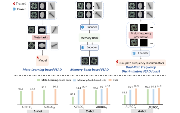
Figure 1: The comparison between DFD and benchmarks. The top figure is previous FSAD framework v.s. ours. Comparison with meta-learning-based FSAD, our model is simple and stability. Comparison with memory-bank-based FSAD, our method needs no extra memory to restore features. The bottle figure is comparison with previous sota performance on MVTec AD dataset for 2-/4-shot setting.

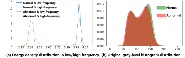
Figure 2: (a) Energy density distribution in low-/high-frequency of tile category, showing that normal/abnormal images obviously differ in frequency distribution. (b) Original gray-level histogram distribution of tile category, showing that normal/abnormal images are hard to distinguish in spatial domain.

Considering the significant resources required for collecting a substantial number of samples and the inherent similarities among industrial images within the same category, there is a growing interest in FSAD  [37, 19, 35, 39, 34, 12] within recent research. FSAD seeks to achieve competitive performance comparable to full-shot anomaly detection methods with only a limited number of (less than 8) source images. As illustrated in Fig. 1, current FSAD methods can be categorized into meta-learning-based methods and memory-bank-based methods. Meta-learning-based FSAD, e.g., RegAD [19] and Metaformer [37] leverage meta-learning strategy to deal with the problem of insufficient training samples. Memory-bank-based [39, 34, 12] methods attempt to employ feature matching for FSAD. However, these methods have some limitations: (1) they have not fully utilized the limited number of training images; (2) subtle anomalies are less noticeable in the spatial domain, and these methods may fail; (3) memory-bank-based methods do not effectively transfer the feature distribution from the images used in pre-trained models to industrial images, and require extra memory bank to store features; (4) meta-learning-based methods have disadvantages of instability during training and enormous computational cost.

In order to solve the aforementioned problems, we propose our Dual-path Frequency Discriminators (DFD) for FSAD. First, we broaden the dataset through plain data augmentation, making the most out of a limited number of samples, and determine the optimal number of augmented samples as show in Fig. 7. Second, instead of directly using the spatial information, we propose to decouple images into different frequency components. High frequencies record fine texture features in an image, while low frequencies are linked to semantic information. Different types of anomalies result in altered information in different frequency bands. Tiny, imperceptible anomalies in the spatial domain are more obvious in the frequency domain. We further tally the information from the MVTev AD dataset in the spatial and frequency domain. Fig. 2 (b) shows that the spatial domain gray-level histogram cannot distinguish normal and abnormal images. However, in Fig. 2 (a) the normal and abnormal images of tile category have different energy distributions at low/high frequencies. The more detalis of Fig. 2 (a) are provided in the supplemental material. Third, we suggest using a feature adaptor to alleviate domain bias and pull normal features together while push the anomaly features apart from normal features. Finally, since abnormal and normal images have distinct feature distributions, it is possible to determine the abnormality directly by applying simple dual-path frequency discriminators without extra memory bank in the feature space. Training a discriminative network solely with normal images can lead to over-fitting, and the discriminative network cannot be optimized due to the lack of positive samples (i.e., anomalous samples). Therefore, we synthesize anomalies at image-level and feature-level to facilitate the dual-path discriminators to consciously distinguish between normal and abnormal features. Our main contributions are summarized as follows:

• We consider anomaly detection as a classification problem in a frequency perspective. We present a novel and stable framework that can make full use of a limited number of source normal images.

• A pseudo-anomaly generation strategy is designed to generate different forms of anomalies at image-level and feature-level. We propose multi-frequency information construction module and fine-grained feature construction module to obtain different frequency adapted features, which are fed into Dual-path feature discrimination module estimating abnormality in latent space.

• We conduct extensive experiments on MVTev and VisA benchmarks, showing that our model performs better than previous FSAD methods. Specifically, our DFD exceeds previous state-of-the-art [21], improving MVTec AD by 1.3% and 1.2% at image-level AUROC and pixel-level AUROC under 2-shot scenarios.

2 Related Work

2.1 Few-shot Learning

Few-shot learning (FSL) pertains to the identification and classification of novel data utilizing an exceedingly limited quantity of training data. FSL methods can be primarily categorised into model fine-tuning, transfer learning, and data augmentation. Fine-tuning methods [31, 27] typically involve pretraining models on large-scale datasets and then fine-tuning the fully connected layers of the model on a target few-shot dataset to obtain the fine-tuned model. Transfer learning methods [36, 20, 13, 40] efficiently transfer the acquired knowledge to a new domain. Data augmentation methods [2, 1, 6] perform data expansion or feature enhancement on the original few-shot dataset.

2.2 Industrial Anomaly Detection

Existing anomaly detection methods can be mainly divided into three types: 1) Reconstruction-based methods primarily hold the perspective that anomalous regions cannot be reconstructed with the architecture of encoders and decoders. Anomaly detection is performed by measuring the reconstruction errors of test samples. Autoencoder (AE), generative adversarial networks (GANs), Transformer, and diffusion model [5, 46, 45, 41, 30, 38, 16, 47] are utilized to reconstruct normal images. 2) Synthesizing-based methods synthesize anomalies on normal samples [25, 45, 18]. CutPaste [25] constructs anomalous images by cutting out portions of anomaly-free images and pasting them onto other locations. The anomalous images in DRÆM [45] are generated using Perlin noise. A reconstructive sub-network is trained to reconstruct the generated anomalous images into normal images, followed by inputting both the reconstructed images and the anomalous images into a segmentation network to predict the anomalous regions. 3) Embedding-based methods typically use a pre-trained network to extract features from samples. These methods discern normal and anomalous features by analyzing extracted shallow features. Mapping the feature distribution obtained from pre-trained models to a multivariate Gaussian distribution is also widely used. DifferNet [33] detects anomaly locations in images by utilizing a normalizing flow-based density estimation of image features at multiple scales. Several other works [15, 43, 24] also employ normalization flow to construct a reversible mapping, from original feature distribution to normal feature distribution. SPADE [9] detects pixel-level anomaly areas according to correspondences based on a multi-resolution feature pyramid. PatchCore [32] proposes an efficient algorithm for striking a balance between retaining a maximum amount of nominal patch features and minimal runtime through coreset subsampling. SimpleNet [29] uses a simple discriminator which is just composed of a 2-layer multi-layer perceptron(MLP), to detect and locate anomalies.

Recently, researchers have been increasingly concerned about FSAD since it only uses a limited number of source anomaly-free samples and can lead to substantial saving cost. The objective of FSAD is to establish competitiveness in comparison to prevailing full-shot anomaly detection methods. Some works [37, 19] leverage the meta-learning paradigm for training, which requires a substantial amount of base data to construct meta-tasks. While others [39, 34, 43, 8] optimize PatchCore [32] for few-shot setting. However, these optimizations have the disadvantage of feature bias. With the success of vision-language models, recent methods have integrated these models into AD. WinCLIP [21] proposes a window-based CLIP framework for anomaly classification and segmentation via fine-grained textual definitions and normal reference samples. This approach has not generalized well to industrial images.

3 Method

The proposed DFD contains 4 parts: anomaly generation (Sec. 3.1), multi-frequency information construction (Sec. 3.2), fine-grained feature construction (Sec. 3.3), and dual-path feature discrimination (Sec. 3.4). We utilize frequency information rather than spatial information, making it easier for the dual-path discriminators network to identify anomalies. The dual-path discriminators can learn joint representation from normal images and pseudo-anomalies. The overview of our method is illustrated in Fig. 3.

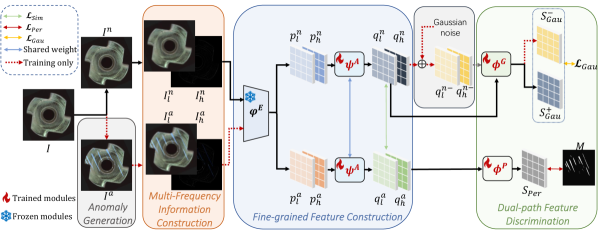
Figure 3: Overview of proposed DFD framework, which mainly consists of: 1) Anomaly Generation module in Sec. 3.1; 2) Multi-Frequency Information Construction module in Sec. 3.2; 3) Fine-grained Feature Construction module in Sec. 3.3; and 4) Dual-path Feature Discrimination module in Sec. 3.4. Input image $I$ is used to generate normal image $I^{n}$ and abnormal image $I^{a}$, which are then decoupled into different frequency components by Multi-Frequency Information Construction module, obtaining $I_{l}^{n}$/$I_{h}^{n}$ and $I_{l}^{a}$/$I_{h}^{a}$. Fine-grained Feature Construction takes above components as inputs that go through a pre-trained feature extractor $\varphi^{E}$ to extract local feature $p_{l}^{n}$/$p_{h}^{n}$ and $p_{l}^{a}$/$p_{h}^{a}$. Subsequent feature adaptor $\psi^{A}$ further transforms local feature to adapted feature $q_{l}^{n}$/$q_{h}^{n}$ and $q_{l}^{a}$/$q_{h}^{a}$. Gaussian noise is added to normal features $q_{l}^{n}$/$q_{h}^{n}$ to get pseudo-anomalous features $q_{l}^{n-}$/$q_{h}^{n-}$. Dual-path Feature Discrimination module contains Gaussian Discriminator $\phi^{G}$ estimating anomalies $S_{Gau}^{-}$ and $S_{Gau}^{+}$ for $q_{l}^{n-}$/$q_{h}^{n-}$ and $q_{l}^{n}$/$q_{h}^{n}$, and Perlin Discriminator $\phi^{P}$ estimating anomalies $S_{Per}$ for $p_{l}^{a}$/$p_{h}^{a}$.

3.1 Anomaly Generation

Anomaly detection assumes that the feature distribution of anomaly-free samples follows a normal distribution. Intuitively, we can construct image-level pseudo-anomalies on normal images. Furthermore, in order to create feature-level pseudo-anomalies that depart from the normal distribution, we introduce noise to the features of normal samples at the feature-level. Hence, we obtain different forms of anomalies from different perspectives during training. The anomaly generation strategy is described below.
Image-level anomaly generation. As shown in Fig. 5, the pseudo-anomalous images are generated based on normal images following DRÆM  [45]. Initially, a original normal image $I\in\mathbb{R}^{H\times W\times 3}$ undergoes binarization to yield a foreground image mask $M_{f}$. Subsequently, a 2-dimensional Perlin noise P is randomly generated, followed by applying a threshold-based binarization to the Perlin noise to generate a mask $M_{p}$. To ensure pseudo-anomalies only appear on the foreground image, an anomaly mask $M$ is generated by performing element-wise product on $M_{f}$ and $M_{p}$ .

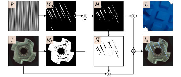
Figure 4: Image-level anomaly generation strategy. The mask $M$ is obtained by performing element-wise product on $M_{p}$ and $M_{f}$ which are generated from random Perlin noise and source normal image. The pseudo-anomalous image is generated from $I$/$I_{t}$ according to $M$.

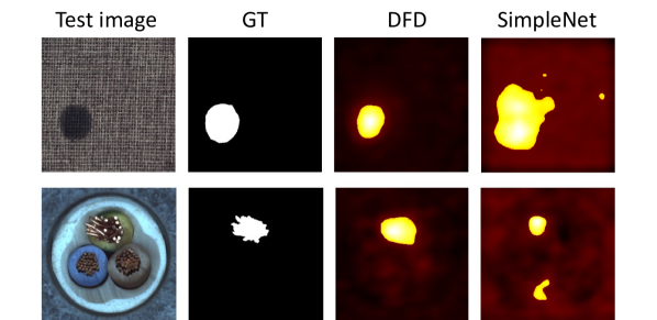
Figure 5: Visualization results of anomaly localization, where test image, ground truth, anomaly map of DFD and anomaly map of SimpleNet for 2-shot setting are shown in MVTec AD dataset.

A texture image $I_{t}$ is then masked with an anomaly mask $M$. To achieve a balanced fusion of the original normal image and the noise image, a transparency factor $\beta$ is introduced, facilitating a closer resemblance of the generated anomaly patterns to real anomalies. Therefore, the generated pseudo-anomalous image $I_{a}$ is defined as:

$$\begin{gathered}I_{a}=\bar{M}\odot I+(1-\beta)\left(M\odot I\right)+\beta\left(M\odot I_{t}\right),\\ M=M_{f}\odot M_{p},\end{gathered}$$ (1)

where $\bar{M}$ is the inverse of $M$.
Feature-level anomaly generation. For feature-level, a Gaussian noise $\epsilon$ is randomly sampled from i.i.d Gaussian distribution $\mathcal{N}(\mu,\sigma^{2})$, which is added to normal features $q_{l}^{n}/q_{h}^{n}\in\mathbb{R}^{h\times w\times C}$ in Sec. 3.3 to obtain pseudo-anomalous features $q_{l}^{n-}/q_{h}^{n-}$ in different frequency components:

$$q_{l}^{n-}=q_{l}^{n}+\epsilon,q_{h}^{n-}=q_{h}^{n}+\epsilon.$$ (2)

3.2 Multi-Frequency Information Construction

Various frequency components encompass distinct information, and different anomalies result in altered information within specific frequency bands. As shown in Fig. 2, normal and abnormal samples have different energy distributions at low/high frequencies. Thus, in contrast to the spatial domain, the frequency domain would offer a fresh viewpoint for anomaly detection.

Given an image $I^{{}^{\prime}}$, we convolve it with a Gaussian kernel. Then remove all even rows and even columns to obtain intermediate image $I_{inter}$. We denote the above process as $\mathrm{Down}$. Next, we perform operation $\mathrm{Up}$. We expand the image $I_{inter}$ by twice its original size in each dimension, filling new rows and columns (even rows and columns) with zeros. Subsequently, convolution is performed to approximate missing pixels with a Gaussian kernel. Then, the low-frequency image $I_{l}$ is acquired:

$$I_{l}=\mathrm{Up}(\mathrm{Down}(I^{{}^{\prime}})).$$ (3)

To recover the missing information, we compute the difference between the image $I^{{}^{\prime}}$ and low-frequency image $I_{l}$, which is represented as follows:

$$I_{h}=I^{{}^{\prime}}-I_{l}.$$ (4)

We carry out above operations for both normal and pseudo-anomalous images, getting thier multi-frequency information $I_{l}^{n}$/$I_{h}^{n}$ and $I_{l}^{a}$/$I_{h}^{a}$.

3.3 Fine-grained Feature Construction

A feature extractor $\varphi^{E}$ and a feature adaptor $\psi^{A}$ make up the fine-grained feature construction module, which is anticipated to obtain adapted features for industrial images.

Following PatchCore [32], we use a pre-trained WideResnet-50 [44] as the feature extractor $\varphi^{E}$ to extract local features for multi-frequency information $I_{l}^{n}$/$I_{h}^{n}$ and $I_{l}^{a}$/$I_{h}^{a}$ from both normal images and pseudo-anomalous images. However, since the pre-training dataset exhibits different distributions from industrial images, we incorporate a feature adaptor $\psi^{A}$ to mitigate the domain bias. Taking the low-frequency component of a normal image $I_{l}^{n}$ as an example, the adapted feature is defined as follows:

$$p_{l}^{n}=\varphi^{E}(I_{l}^{n}),q_{l}^{n}=\psi^{A}(p_{l}^{n}),\\$$ (5)

where $p_{l}^{n}$ is the local features. Through the aforementioned process, we get the adapted feature $q_{l}^{n}$/$q_{h}^{n},q_{l}^{a}$/$q_{h}^{a}\in\mathbb{R}^{h\times w\times C}$.

3.4 Dual-path Feature Discrimination

Both the feature distributions of the normal and abnormal samples differ, and the adapted features provide spatial information. Taking anomaly detection as a feature space classification problem allows us to assess the abnormality of adapted features effectively. We present a dual-path feature discrimination module, comprising a Gaussian discriminator $\phi^{G}$ and a Perlin discriminator $\phi^{P}$, to identify pseudo-anomalies produced in the feature space at both the feature-level and image-level.

Gaussian Discriminator. In this branch, the normal adapted features $q_{l}^{n}$/$q_{h}^{n}\in\mathbb{R}^{h\times w\times C}$ and pseudo-anomalous features $q_{l}^{n-}$/$q_{h}^{n-}\in\mathbb{R}^{h\times w\times C}$ are forwarded to Gaussian Discriminator $\phi^{G}$ to estimate the abnormality at each position $(h,w)$. The output $\phi^{G}(q)\in\mathbb{R}$ of Gaussian Discriminator is positive for normal features while negative for pseudo-anomalous features. The Gaussian discriminator $\phi^{G}$ is just constructed using a 2-layer multi-layer perceptron (MLP) structure.

Perlin Discriminator. Vision Transformer (ViT) utilizes the self-attention mechanism to capture global long-term dependency enabling the model to understand contextual relationships across the entire image. Moreover, ViT is able to recognize intricate patterns and details  [17, 22]. These attributes are beneficial for comprehending anomalies in industrial scenarios. Similar to the Gaussian Discriminator $\phi^{G}$, the output of the Perlin Discriminator $\phi^{P}(q)\in\mathbb{R}$ is expected to be positive for normal features while negative for abnormal features at each position $(h,w)$. We combine a single-layer MLP and a single-layer ViT as the Perlin Discriminator $\phi^{P}$.

3.5 Training Objectives

We propose three losses for training DFD in Fig. 3.

Similarity loss. In order to push the anomalous features apart from normal features and pull the normal features together, the similarity loss $\mathcal{L}_{Sim}$ is utilized between pseudo-anomalous images and normal images at corresponding positions:

$$\left\{\begin{aligned} \mathcal{L}_{l_{Sim}}&=1-\cos(M^{\prime}\odot q_{l}^{a},M^{\prime}\odot q_{l}^{n}),\\ \mathcal{L}_{h_{Sim}}&=1-\cos(M^{\prime}\odot q_{h}^{a},M^{\prime}\odot q_{h}^{n}),\\ \mathcal{L}_{Sim}&=\mathcal{L}_{l_{Sim}}+\mathcal{L}_{h_{Sim}},\end{aligned}\right.$$ (6)

where $M^{\prime}\in\mathbb{R}^{h\times w}$ is yielded by applying max pooling to $M\in\mathbb{R}^{H\times W}$ in Eq. 1. During training, we encourage feature adaptor to separate normal features from anomaly features, with normal features being compact. Strong differences between the pseudo-anomalous and normal images are ensured by optimizing $\mathcal{L}_{Sim}$.

Gaussian loss. Gaussian loss penalizes negative scores for normal features and positive for pseudo-anomalous features following. We use truncated $l_{1}$ loss as Gaussian loss:

$$\left\{\begin{aligned} \mathcal{L}_{l_{Gau}}&=\max\{0,\theta-\phi^{G}(q_{l}^{n})\}+\max\{0,\theta+\phi^{G}(q_{l}^{n-})\},\\ \mathcal{L}_{h_{Gau}}&=\max\{0,\theta-\phi^{G}(q_{h}^{n})\}+\max\{0,\theta+\phi^{G}(q_{h}^{n-})\},\\ \mathcal{L}_{Gau}&=\mathcal{L}_{l_{Gau}}+\mathcal{L}_{h_{Gau}},\end{aligned}\right.$$ (7)

where $\theta$ is set to 0.8 by default preventing over-fitting.

Perlin loss. First, we use truncated $l_{1}$ loss to ensure that Perlin Discriminator $\phi^{P}$ can locate the generated pseudo-anomalous regions:

$$\mathcal{L}_{l_{pix}}=\max\{0,\theta-\phi^{P}(q_{l}^{a})\odot(1-M^{\prime})\}+\max\{0,\theta+\phi^{P}(q_{l}^{a})\odot M^{\prime}\}.$$ (8)

The high-frequency loss $\mathcal{L}_{h_{pix}}$ is similar to Eq. 8. Consequently, the pixel loss is defined as:

$$\mathcal{L}_{pix}=\mathcal{L}_{l_{pix}}+\mathcal{L}_{h_{pix}}.$$ (9)

What’s more, we take the maximum value of the output of $\phi^{P}$ and use a simple $l2$ loss to estimate abnormality for the image:

$$\ \left\{\begin{aligned} \mathcal{L}_{l_{cls}}&=||\tau-{\max}\{\mathrm{Sigmoid}(-\phi(q_{l}^{a}))\}||^{2},\\ \mathcal{L}_{h_{cls}}&=||\tau-{\max}\{\mathrm{Sigmoid}(-\phi(q_{h}^{a}))\}||^{2},\\ \mathcal{L}_{cls}&=\mathcal{L}_{l_{cls}}+\mathcal{L}_{h_{cls}},\end{aligned}\right.$$ (10)

where $\tau$ is the ground truth of the image abnormality. The overall Perlin loss $\mathcal{L}_{\text{Per }}$ is defined as :

$$\mathcal{L}_{\text{Per}}=\frac{1}{2}(\mathcal{L}_{\text{pix}}+\mathcal{L}_{\text{cls}}).$$ (11)

In summary, the total loss is defined as:

$$\mathcal{L}=\mathcal{L}_{\text{Gau}}+\lambda_{Per}\mathcal{L}_{\text{Per}}+\lambda_{Sim}\mathcal{L}_{\text{Sim}}.$$ (12)

3.6 Inference

As depicted in Fig. 3, we discard the process of generating anomalies at image-level and feature-level. For a test image $I_{test}\in\mathbb{R}^{H\times W\times 3}$, we obtain the low-/high-frequency adapted features $q^{l}/q^{h}\in\mathbb{R}^{h\times w\times C}$. Gaussian Discriminator $\phi^{G}$ and Perlin Discriminator $\phi^{P}$ calculate the anomaly scores $S_{Gau},S_{Per}\in\mathbb{R}^{h\times w}$ for $q^{l}$/$q^{h}$ simultaneously:

$$S_{Gau}=\phi^{G}(q^{l})+\phi^{G}(q^{h}),S_{Per}=\phi^{P}(q^{l})+\phi^{P}(q^{h}).$$ (13)

We scale above anomaly scores to [0, 1]:

$$S^{\prime}_{Gau}=\frac{S_{Gau}-{\min}(S_{Gau})}{{\max}(S_{Gau})-{\min}(S_{Gau})},S^{\prime}_{Per}=\frac{S_{Per}-{\min}(S_{Per})}{{\max}(S_{Per})-{\min}(S_{Per})}.$$ (14)

Then the anomaly scores of a test image is acquired by averaging $S^{\prime}_{Gau}\in\mathbb{R}^{h\times w}$ and $S^{\prime}_{Per}\in\mathbb{R}^{h\times w}$:

$$S^{\prime}=\frac{1}{2}(S^{\prime}_{Gau}+S^{\prime}_{Per}).$$ (15)

$S^{\prime}\in\mathbb{R}^{h\times w}$ is interpolated to obtain the final anomaly score map $S\in\mathbb{R}^{H\times W}$. The anomaly detection score $S_{A}$ for each test image is determined by selecting the maximum score of $S$.

4 Experiments

4.1 Experimental Setups

Datasets. We conduct a range of experiments on MVTec AD [3] and VisA [48]. MVTec AD consists of a total of 15 categories and 5,354 images, with 3,629 images for training and 1,725 images for testing. The training data comprises only normal images, while the testing data includes both normal and anomaly images. VisA contains 12 categories and 10,821 images, with 9621 normal and 1,200 anomalous samples. Our method is consistent with previous FSAD methods in the use of only normal samples.

Evaluation metrics. For evaluating the performance of sample-level anomaly detection, we use Area Under the Receiver Operator Curve (AUROC_i). For anomaly localization, pixel-wise AUROC (AUROC_p) and Per-Region Overlap (PRO) are used as evaluation metrics.

Implementation details. All experiments are implemented on an RTX 3090 GPU. In our experiments setting, we randomly choose normal samples from source samples for few-shot setting, and we resize all images to $256\times 256$ resolution. We adopt pre-trained models with ImageNet [11] as backbones. By default, we use WideResNet-50 as the backbone following SimpleNet [29] and choose features of level 2 + 3 as local features following [32]. We employ Adam optimizer [23], setting the learning rate to 5e-4 for the feature adaptor, 2e-4 for the Gaussian discriminator, and 1e-4 for the Perlin discriminator. In Eq. 12, we set $\lambda_{Per}=2$, $\lambda_{Sim}=0.02$ for MVTec AD [3], and $\lambda_{Per}=1$, $\lambda_{Sim}=1$ for VisA [48]. We set training epochs to 80 and batchsize to 8.

4.2 Experimental Results

Table 1: Comparison of average FSAD performance on MVTec AD and VisA dataset. Bold and underline represent optimal and sub-optimal results, respectively.

Dataset	Method	1-shot			2-shot			4-shot
		AUROCi	AUROCp	PRO	AUROCi	AUROCp	PRO	AUROCi	AUROCp	PRO
MVTec	SPADE [9]	81.0	91.2	83.9	82.9	92.0	85.7	84.8	92.7	87.0
	PaDiM [10]	76.6	89.3	73.3	78.9	91.3	78.2	80.4	92.6	81.3
	RegAD [19]	-	-	-	85.7	94.6	-	88.2	95.8	-
	PatchCore [32]	83.4	92.0	79.7	86.3	93.3	82.3	88.8	94.3	84.3
	GraphCore [39]	89.9	95.6	-	91.9	96.9	-	92.9	97.4	-
	WinCLIP [21]	93.1	95.2	87.1	94.4	96.0	88.4	95.2	96.2	89.0
	FastRecon [12]	-	-	-	91.0	95.9	-	94.2	97.0	-
	AnomalyGPT [14]	94.1	95.3	-	95.5	95.6	-	96.3	96.2	-
	Ours	93.3	96.2	88.4	95.7	97.2	88.9	96.9	97.5	89.9
VisA	SPADE [9]	79.5	95.6	84.1	80.7	96.2	85.7	81.7	96.6	87.3
	PaDiM [10]	62.8	89.9	64.3	67.4	92.0	70.1	72.8	93.2	72.6
	PatchCore [32]	79.9	95.4	80.5	81.6	96.1	82.6	85.3	96.8	84.9
	WinCLIP [21]	83.8	96.4	85.1	84.6	96.8	86.2	87.3	97.2	87.6
	AnomalyGPT [14]	87.4	96.2	-	88.6	96.4	-	90.6	96.7	-
	Ours	84.2	96.8	86.2	87.4	97.1	86.3	88.7	97.2	86.8

Few-shot anomaly detection and localization. We compare our DFD with prior methods specifically designed for few-shot setting. In Tab. 1, we illustrate average experimental results for MVTec AD [3] and VisA [48]. 1) For few-shot anomaly detection, across both datasets, our method DFD outperforms prior works. Specifically, we improve AUROC_i upon the current sota FSAD approach WinClip [21] by +0.2%, +1.3%, +1.5% on MVTec AD and +0.4%, +2.8%, +1.5% on VisA for 1, 2, 4-shot setting, respectively. 2) For few-shot anomaly localization, we improve AUROC_p upon WinClip [21] by +1.0%, +1.2%, +1.3% on MVTec AD and +0.4%, +0.3%, +0.0% on VisA for 1, 2, 4-shot setting. The visualization results of anomaly localization in Fig. 5 further demonstrates the accuracy of our method in localizing anomalies, where SimpleNet [29] is our baseline method.

Comparison with full-shot methods. In Tab. 2, we compare our method with full-shot anomaly detection methods. The results show that the proposed DFD is competitive with full-shot methods. In particular, our 4-shot AUROC_p outperforms DRÆM that uses whole normal samples.

Table 2: Comparison with full-shot methods in AUROC_i and AUROC_p on MVTec AD dataset.

Model	Setting	AUROCi	AUROCp
DFD (Ours)	1-shot	93.3	96.2
	2-shot	95.7	97.2
	4-shot	96.9	97.5
SimpleNet [29]	full-shot	99.6	98.1
PatchCore [32]	full-shot	99.1	98.1
CFLOW [15]	full-shot	98.3	98.6
DRÆM [45]	full-shot	98.0	97.3

Table 3: Performance with the configuration of different components.

Gaussian-Disc	Perlin-Disc	DA	MFIC	$\mathcal{L}_{Sim}$	AUROCi	AUROCp	PRO
✓	✗	✗	✗	✗	77.5	74.4	47.9
✓	✓	✗	✗	✗	79.6	85.3	61.3
✓	✓	✓	✗	✗	91.6	95.1	84.6
✓	✓	✓	✓	✗	93.7	96.3	88.9
✓	✓	✓	✗	✓	93.1	96.5	88.0
✓	✗	✓	✓	✓	92.9	96.4	86.2
✗	✓	✓	✓	✓	94.0	93.4	83.7
✓	✓	✓	✓	✓	95.7	97.2	88.9

Table 4: Ablation study of different frequency information.

Model	AUROCi	AUROCp	PRO
Ours	95.7	97.2	88.9
W/o MFIC	93.3	96.2	70.3
Only high-frequency	92.5	94.2	80.4
Only low-frequency	91.7	94.1	73.6

Table 5: Ablation study of different forms of anomalies.

Model	AUROCi	AUROCp	PRO
Ours	95.7	97.2	88.9
W/o pseudo-anomalies	59.7	36.3	88.9
Image-level anomalies	91.3	87.4	39.1
Feature-level anomaliesy	83.7	91.4	70.7

4.3 Ablation Study

In this section, we verify the effectiveness of proposed various modules. We conduct extensive experiments on MVTec AD dataset [3] for 2-shot setting following prior work [39].

Influence of different components. We conduct the following experiments: (1) Baseline (SimpleNet [29], i.e. Gaussian Discriminator and pseudo-anomalies at feature-level), denoted as Gaussian-Disc; (2) Adding Perlin Discriminator and pseudo-anomalies at image-level, denoted as Perlin-Disc ; (3) Adding both Perlin-Disc and data augmentation (DA); (4) Adding multi-frequency information construction (MFIC) module to (3); (5) Adding similarity loss ($\mathcal{L}_{Sim}$) to (3); (6) Proposed DFD without Perlin-Disc; (7) Proposed DFD without Gaussian-Disc; (8) Proposed DFD in this paper. As shown in Tab. 3, our baseline (SimpleNet [29]) only obtains 77.5%/74.4% AUROC_i/AUROC_p because of its poor utilization of a limited number of normal images. Training with our Perlin Discriminator can increase the AUROC_i/AUROC_p by +2.1%/+10.9%. When we add DA which is used to expand dataset to above modules, the performance increases by +12.0%/+9.8%. Subsequently, adding MFIC module improves by +2.7%/+1.2%. Introducing similarity loss ($\mathcal{L}_{Sim}$) can enhance performance by an additional +2.0%/+0.9%. The other loss functions are specifically tailored to guide the training of their respective discriminators, thus obviating the need for additional experimental validation of their efficacy. Tab. 3 shows that each module added improves model performance.

Influence of different frequency information. Different frequency components of an image represent different information. As shown in Tab. 5, we conduct a range of experiments to investigate the impact of using different frequencies on performance of anomaly detection: (1) proposed DFD; (2) without multi-frequency information construction; (3) only high-frequency; (4) only low-frequency. Using only high-frequency information of the image demonstrates superior performance compared to using only low-frequency information. Using the original image performs better than using high-/low-frequency information alone. However, incorporating high-frequency and low-frequency information performs the best, meaning the normal images and abnormal images contain different frequency information.

Influence of dual-path discriminators. We run separate experiments using different discriminators and present the results in rows 6 and 7 of Tab. 3. The performance of using one discriminator individually has deteriorated in comparison to using dual-path discriminators.

Table 6: Ablation study of different loss function.

Model	AUROCi	AUROCp	PRO
Ours	95.7	97.2	88.9
Ours-CE	94.0	96.8	84.0
Ours-Focal	94.8	96.3	82.0
Ours-MSE	93.6	96.2	88.6

Influence of different forms of anomalies. The introduction of pseudo-anomalies at both the image and feature levels exerts significant influence for our dual-path discriminators to learn a joint representation of anomalous features and normal features. As illustrated in Tab. 5, the omission of any specific anomalies can result in a deterioration of the outcomes. The feature representation learned by the discriminators during training fails to grasp the intricacies of the anomalies. The malfunctioning of any of the discriminators has the potential to negatively impact the overall experimental outcomes, resulting in a decline in the final results.

Influence of feature adaptor and similarity loss. The pre-trained backbone utilizes the ImageNet [11], which significantly differs from industrial images. We use a feature adaptor in fine-grained feature construction module to reduce domain bias by different distributions. We count the feature distribution with/without feature adaptor. In Fig. 6 the features with a feature adaptor becomes more compact. Moreover, different from SimpleNet [29], a similarity loss $\mathcal{L}_{Sim}$ is expected to push normal features apart from normal features. As shown in Fig. 6, we further visualize the normal features and abnormal features distribution. The boundary between normal and abnormal distributions is clearly explicit with the feature adaptor. In Tab. 3 quantitative results also illustrate our similarity loss $\mathcal{L}_{Sim}$ plays a demonstrative role for AD performance.

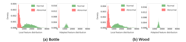
Figure 6: Log-likelihood histograms from bottle and wood category. Left is local feature without adaptor, right is the adapted features with adaptor.

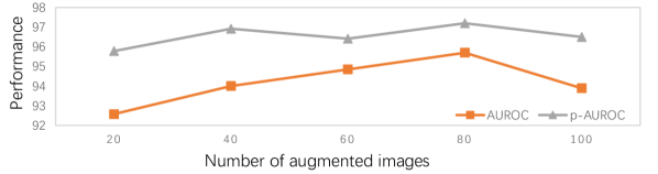
Figure 7: Performance of the number of augmented images per source normal image.

Influence of loss function. The commonly used classification loss function and proposed the truncated $l_{1}$ loss were compared. We replaced the truncated $l_{1}$ loss of Gaussian loss $\mathcal{L}_{Gau}$ in Eq. 7 and pixel loss in Eq. 9, with cross-entropy loss, focal loss, and MSE loss, denoted as "Ours-CE," "Ours-Focal," and "Ours-MSE" respectively. The results depicted in Tab. 6 clearly demonstrate that our truncated $l_{1}$ loss yields the most favorable outcomes

The number of augmented images. We investigate the influence of the number of augmented images per normal image. As shown in Fig. 7, within a certain range, an increased quantity of augmented images correlates positively with enhanced performance. However, when the number becomes excessively large, the performance may deteriorate. Thus we choose the number of augmented images $N=80$.

5 Conclusion and Future Works

Conclusion. In this paper, we propose a novel and simple DFD approach from a frequency perspective for few-shot anomaly detection. We generate anomalies at both image-level and feature-level for full use of a limited number of source normal images. To better train feature adaptor, we propose a similarity loss to push normal features apart from abnormal features. We further employ dual-path discriminators to estimate abnormality for two different forms of anomalies. In the end, our DFD network has the ability to learn a joint representation of the features of both normal and abnormal images.

Limitation. Although our method DFD exhibits favorable performance, generated pseudo-anomalies at image-level and feature-level still differ from real anomalies on industrial images. Data augmentation for each source normal images would increase the training time and may make the model over-fitting.

Future Works. In the future, we will continue to explore industrial few-shot anomaly detection. We aim to fully utilize the limited number of normal images and improve the adaptability for other anomaly detection scenarios.

Supplementary Material

Dual-path Frequency Discriminators for
Few-shot Anomaly Detection

Appendix 0.A Experimental details

Energy density distribution. In Fig. 2 (a), we perform a two-dimensional Fourier transform on the image to obtain a complex matrix with the same size as the image. To analyze frequency information more intuitively, the matrix is “frequency centered”, wherein low-frequency components are positioned at the matrix center surrounded by high-frequency components. For matrix elements at coordinates (x,y), their Euclidean distance from the center implies frequency value, and the modulus of the complex number represents energy. Due to the conjugate property of the two-dimensional Fourier transform, the amplitude spectrum obtained above is symmetric about the center. The energy distribution curve is plotted with the abscissa representing the distance from the point to the center (frequency) and the ordinate representing the amplitude value (energy). We categorize the images within the MVTec dataset into two distinct classes: texture images, including carpets, and object images, comprising items like capsules. In Figure 2, the frequency distributions of images a and b from these respective categories are illustrated. Notably, disparities in frequency information between normal and abnormal images exist within each category, yet the specific patterns of these differences diverge.

Data Augmentation. We generate pseudo-anomalous images in Sec. 3.1 for data augmentation. A training normal image is randomly rotated within (-90, 90) degrees, and then performed image-level anomaly generation strategy in Eq. 1 with a probability of 70%. It performs a channel-wise standardization with the mean [0.485, 0.456, 0.406] and standard deviation [0.229, 0.224, 0.225]. We will obtain $N=80$ pseudo-anomalous images by above process.

The specific structure of each part. A pre-trained WideResnet-50 is employed as the feature extractor $\varphi^{E}$. We choose features of level $2+3$ as local features following PatchCore [32]. Moreover, the feature adaptor $\psi^{A}$ consists of a single linear layer. We use a 2-layer MLP sturcture as the Gaussian discriminator $\phi^{G}$. While the Perlin discriminator $\phi^{P}$ consists of a single-layer MLP and a single-layer ViT. And we set num_heads to 16 for ViT.

Appendix 0.B Additional ablation study

Comparison with SimpleNet. We choose SimpleNet [29] as our baseline, a current state-of-the-art method for full-shot anomaly detection. We further conduct a range of experiments on MVTec AD [3] and VisA [48] dataset for few-shot setting with SimpleNet baseline. As shown in Tab. 7, compared with SimpleNet [29], our proposed DFD has achieved siginificant improvements in various indicators for FSAD.

Table 7: Comparison of average FSAD performance on MVTec AD dataset with SimpleNet. Bold represents optimal results.

Setting	Method	MVTec AD			VisA
		AUROC	p-AUROC	PRO	AUROC	p-AUROC	PRO
1-shot	SimpleNet	76.6	74.1	46.7	57.1	74.0	32.3
	ours	93.3	96.2	88.4	84.2	96.8	86.2
2-shot	SimpleNet	77.5	74.4	47.9	62.9	80.2	38.3
	ours	95.7	97.2	88.9	87.4	97.1	86.3
4-shot	SimpleNet	78.9	80.8	56.8	66.2	81.6	40.5
	ours	96.9	97.5	89.9	88.7	97.2	86.8

Different structures of Perlin Discriminator. We use different structures of Perlin Discriminator, and the results illustrates our improvements, +1.2% AUROC_i, +1.2% AUROC_p, over 2-layer MLP in Tab. 8. A 2-layer MLP is the same with Gaussian Discriminator following SimpleNet [29]. We consider the translation invariance of ViT makes it sensitive to position information. What’s more, ViT can capture global context information. Therefore, for generated pseudo-anomalies at image-level, ViT would locate anomalies more accurately.

Table 8: Ablation of different structures for Perlin Discriminator.

Perlin Discriminator	AUROCi	AUROCp	PRO
A single-MLP + a single-ViT (Ours)	95.7	97.2	88.9
2-layer MLP	94.5	96.0	88.8

Existing drawbacks. In Tab. 7, sometimes the evaluation metrics improve insignificantly from 1-shot to 4-shot setting, which may be due to overfitting. In Tab. 9 and Tab. 10, the performance of each category on MVTec AD and VisA is reported. The performance of certain categories, such as screw and toothbrush in MVTec AD, capsules and macaroni2 in VisA, is mediocre. The major factor causing the results is the anomaly generation in Sec. 3.1. The pseudo-anomalies generated in Eq. 1 are more consistent with surface anomalies, e.g. scratches. Capsules, candles and macaronis, etc. have multiple objects, generated pseudo-anomalous areas cannot cover all objects. What’s more, the features of actual anomalies in the manufacturing production do not strictly satisfy the Gaussian distribution. Logical anomaly like misplacement or missing parts cannot be simulated by generated pseudo-anomalies at both image-level and feature-level.

Appendix 0.C Additional detailed quantitative results

In this section, we present the performance for each category on MVTec AD and VisA dataset. The detailed results for 1, 2, 4-shot setting are shown in Tab. 9 and Tab. 10.

Appendix 0.D Additional detailed qualitative results

In this section, we report our qualitative results on MVTec AD and VisA dataset in Figs. 8, 9, 10 and 11.

Table 9: Quantitative results on MVTec AD dataset.

Object	1-shot			2-shot			4-shot
	AUROC	p-AUROC	PRO	AUROC	p-AUROC	PRO	AUROC	p-AUROC	PRO
bottle	99.3	97.9	93.2	99.7	98.1	93.8	99.9	98.3	92.5
cable	89.9	92.0	82.6	90.3	92.3	82.3	97.2	93.1	85.6
capsule	81.5	94.6	87.9	86.3	97.1	88.5	94.7	97.5	89.9
carpet	99.8	99.1	94.3	99.9	99.1	92.2	99.9	99.0	92.8
grid	94.6	96.1	86.0	98.8	98.4	91.4	99.0	98.4	94.9
hazelnut	99.5	98.5	95.2	100.0	99.0	96.2	100.0	99.1	96.5
leather	100.0	99.6	98.4	100.0	99.5	98.5	100.0	99.6	98.
metal_nut	98.2	97.4	92.8	98.9	98.0	93.7	99.0	98.3	90.0
pill	95.7	99.0	96.4	95.8	99.0	94.6	96.9	99.2	94.5
screw	80.3	97.3	85.1	86.5	94.5	87.1	85.2	96.6	87.9
tile	100.0	98.6	92.0	100.0	99.0	92.2	100.0	99.2	94.4
toothbrush	81.4	97.3	77.6	88.3	96.8	67.5	88.3	97.6	76.3
transistor	87.2	81.1	61.8	91.7	88.8	72.9	97.0	90.1	68.6
wood	99.5	96.3	90.3	99.5	96.3	91.7	99.3	97.3	91.2
zipper	92.7	98.2	91.7	99.4	98.2	91.6	97.3	98.6	95.4
Mean	93.3	96.2	88.4	95.7	97.2	88.9	96.9	97.5	89.9

Table 10: Quantitative results on VisA dataset.

Object	1-shot			2-shot			4-shot
	AUROC	p-AUROC	PRO	AUROC	p-AUROC	PRO	AUROC	p-AUROC	PRO
candle	82.8	98.0	93.3	85.7	98.2	90.4	93.3	96.4	92.1
capsules	66.4	95.9	68.6	74.3	96.9	81.2	78.0	97.1	70.8
cashew	94.8	98.9	89.7	95.3	98.1	79.8	92.7	96.8	87.3
chewinggum	97.6	99.2	87.7	98.3	99.0	75.8	97.9	98.7	86.0
fryum	94.4	95.6	84.4	96.6	95.4	87.2	91.6	96.9	86.8
macaroni1	84.3	99.1	95.2	88.4	98.9	96.2	92.7	98.5	94.2
macaroni2	56.7	97.4	87.0	63.9	96.2	87.7	65.9	98.2	91.5
pcb1	93.4	96.5	86.6	89.5	97.2	86.5	91.4	96.8	87.3
pcb2	76.0	93.6	78.2	84.6	94.7	84.7	83.3	96.0	82.3
pcb3	78.4	95.2	86.2	86.4	93.5	85.5	87.5	95.7	87.3
pcb4	89.7	93.7	82.1	91.7	97.3	86.2	94.7	96.4	81.9
pipe_fryum	95.8	99.0	95.9	94.0	99.3	94.4	94.9	99.4	93.9
Mean	84.2	96.8	86.2	87.4	97.1	86.3	88.7	97.3	86.8

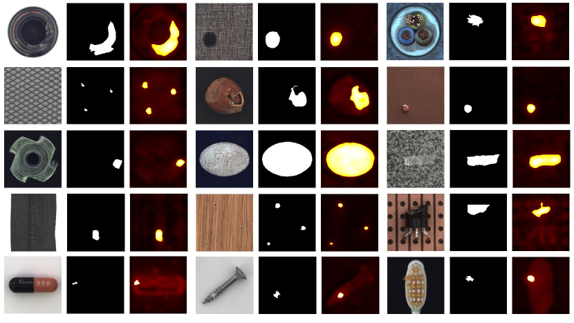
Figure 8: Visualization results of anomaly localization, where test image, ground truth, anomaly map are shown in MVTec AD dataset.

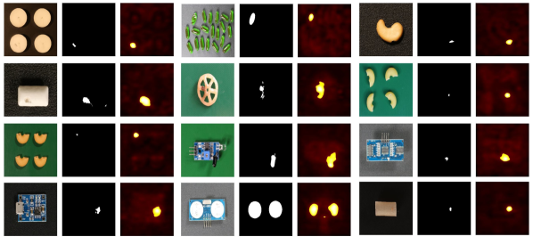
Figure 9: Visualization results of anomaly localization, where test image, ground truth, anomaly map are shown in VisA dataset.

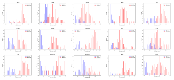
Figure 10: Histogram of anomaly scores for the normal and abnormal samples on the MVTec AD dataset.

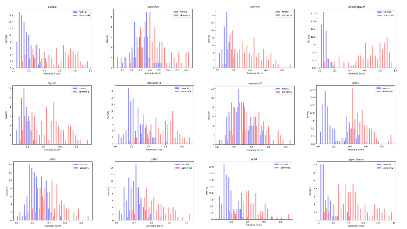
Figure 11: Histogram of anomaly scores for the normal and abnormal samples on the VisA dataset.

References

- [1] Aksu, T., Liu, Z., Kan, M.Y., Chen, N.F.: N-shot learning for augmenting task-oriented dialogue state tracking. arXiv preprint arXiv:2103.00293 (2021)
- [2] Benaim, S., Wolf, L.: One-shot unsupervised cross domain translation. advances in neural information processing systems 31 (2018)
- [3] Bergmann, P., Fauser, M., Sattlegger, D., Steger, C.: Mvtec ad–a comprehensive real-world dataset for unsupervised anomaly detection. In: Proceedings of the IEEE/CVF conference on computer vision and pattern recognition. pp. 9592–9600 (2019)
- [4] Bergmann, P., Fauser, M., Sattlegger, D., Steger, C.: Uninformed students: Student-teacher anomaly detection with discriminative latent embeddings. In: Proceedings of the IEEE/CVF conference on computer vision and pattern recognition. pp. 4183–4192 (2020)
- [5] Bergmann, P., Löwe, S., Fauser, M., Sattlegger, D., Steger, C.: Improving unsupervised defect segmentation by applying structural similarity to autoencoders. arXiv preprint arXiv:1807.02011 (2018)
- [6] Boudiaf, M., Ziko, I., Rony, J., Dolz, J., Piantanida, P., Ben Ayed, I.: Information maximization for few-shot learning. Advances in Neural Information Processing Systems 33, 2445–2457 (2020)
- [7] Cao, Y., Xu, X., Zhang, J., Cheng, Y., Huang, X., Pang, G., Shen, W.: A survey on visual anomaly detection: Challenge, approach, and prospect. arXiv preprint arXiv:2401.16402 (2024)
- [8] Chen, X., Zhang, J., Tian, G., He, H., Zhang, W., Wang, Y., Wang, C., Wu, Y., Liu, Y.: Clip-ad: A language-guided staged dual-path model for zero-shot anomaly detection. arXiv preprint arXiv:2311.00453 (2023)
- [9] Cohen, N., Hoshen, Y.: Sub-image anomaly detection with deep pyramid correspondences. arXiv preprint arXiv:2005.02357 (2020)
- [10] Defard, T., Setkov, A., Loesch, A., Audigier, R.: Padim: a patch distribution modeling framework for anomaly detection and localization. In: International Conference on Pattern Recognition. pp. 475–489. Springer (2021)
- [11] Deng, J., Dong, W., Socher, R., Li, L.J., Li, K., Fei-Fei, L.: Imagenet: A large-scale hierarchical image database. In: 2009 IEEE conference on computer vision and pattern recognition. pp. 248–255. Ieee (2009)
- [12] Fang, Z., Wang, X., Li, H., Liu, J., Hu, Q., Xiao, J.: Fastrecon: Few-shot industrial anomaly detection via fast feature reconstruction. In: Proceedings of the IEEE/CVF International Conference on Computer Vision. pp. 17481–17490 (2023)
- [13] Finn, C., Abbeel, P., Levine, S.: Model-agnostic meta-learning for fast adaptation of deep networks. In: International conference on machine learning. pp. 1126–1135. PMLR (2017)
- [14] Gu, Z., Zhu, B., Zhu, G., Chen, Y., Tang, M., Wang, J.: Anomalygpt: Detecting industrial anomalies using large vision-language models. arXiv preprint arXiv:2308.15366 (2023)
- [15] Gudovskiy, D., Ishizaka, S., Kozuka, K.: Cflow-ad: Real-time unsupervised anomaly detection with localization via conditional normalizing flows. In: Proceedings of the IEEE/CVF Winter Conference on Applications of Computer Vision. pp. 98–107 (2022)
- [16] He, H., Zhang, J., Chen, H., Chen, X., Li, Z., Chen, X., Wang, Y., Wang, C., Xie, L.: Diad: A diffusion-based framework for multi-class anomaly detection. In: AAAI (2024)
- [17] He, J., Chen, J.N., Liu, S., Kortylewski, A., Yang, C., Bai, Y., Wang, C.: Transfg: A transformer architecture for fine-grained recognition. arXiv preprint arXiv:2103.07976 (2021)
- [18] Hu, T., Zhang, J., Yi, R., Du, Y., Chen, X., Liu, L., Wang, Y., Wang, C.: Anomalydiffusion: Few-shot anomaly image generation with diffusion model. In: AAAI (2024)
- [19] Huang, C., Guan, H., Jiang, A., Zhang, Y., Spratling, M., Wang, Y.F.: Registration based few-shot anomaly detection. In: European Conference on Computer Vision. pp. 303–319. Springer (2022)
- [20] Jang, Y., Lee, H., Hwang, S.J., Shin, J.: Learning what and where to transfer. In: International conference on machine learning. pp. 3030–3039. PMLR (2019)
- [21] Jeong, J., Zou, Y., Kim, T., Zhang, D., Ravichandran, A., Dabeer, O.: Winclip: Zero-/few-shot anomaly classification and segmentation. In: Proceedings of the IEEE/CVF Conference on Computer Vision and Pattern Recognition. pp. 19606–19616 (2023)
- [22] Khan, S., Naseer, M., Hayat, M., Zamir, S.W., Khan, F.S., Shah, M.: Transformers in vision: A survey. ACM computing surveys (CSUR) 54(10s), 1–41 (2022)
- [23] Kingma, D.P., Ba, J.: Adam: A method for stochastic optimization. arXiv preprint arXiv:1412.6980 (2014)
- [24] Lei, J., Hu, X., Wang, Y., Liu, D.: Pyramidflow: High-resolution defect contrastive localization using pyramid normalizing flow. In: Proceedings of the IEEE/CVF Conference on Computer Vision and Pattern Recognition. pp. 14143–14152 (2023)
- [25] Li, C.L., Sohn, K., Yoon, J., Pfister, T.: Cutpaste: Self-supervised learning for anomaly detection and localization. In: Proceedings of the IEEE/CVF conference on computer vision and pattern recognition. pp. 9664–9674 (2021)
- [26] Liang, Y., Zhang, J., Zhao, S., Wu, R., Liu, Y., Pan, S.: Omni-frequency channel-selection representations for unsupervised anomaly detection. IEEE Transactions on Image Processing (2023)
- [27] Liu, H., Tam, D., Muqeeth, M., Mohta, J., Huang, T., Bansal, M., Raffel, C.A.: Few-shot parameter-efficient fine-tuning is better and cheaper than in-context learning. Advances in Neural Information Processing Systems 35, 1950–1965 (2022)
- [28] Liu, J., Xie, G., Wang, J., Li, S., Wang, C., Zheng, F., Jin, Y.: Deep industrial image anomaly detection: A survey. MIR (2024)
- [29] Liu, Z., Zhou, Y., Xu, Y., Wang, Z.: Simplenet: A simple network for image anomaly detection and localization. In: Proceedings of the IEEE/CVF Conference on Computer Vision and Pattern Recognition. pp. 20402–20411 (2023)
- [30] Mishra, P., Verk, R., Fornasier, D., Piciarelli, C., Foresti, G.L.: Vt-adl: A vision transformer network for image anomaly detection and localization. In: 2021 IEEE 30th International Symposium on Industrial Electronics (ISIE). pp. 01–06. IEEE (2021)
- [31] Nakamura, A., Harada, T.: Revisiting fine-tuning for few-shot learning. arXiv preprint arXiv:1910.00216 (2019)
- [32] Roth, K., Pemula, L., Zepeda, J., Schölkopf, B., Brox, T., Gehler, P.: Towards total recall in industrial anomaly detection. In: Proceedings of the IEEE/CVF Conference on Computer Vision and Pattern Recognition. pp. 14318–14328 (2022)
- [33] Rudolph, M., Wandt, B., Rosenhahn, B.: Same same but differnet: Semi-supervised defect detection with normalizing flows. In: Proceedings of the IEEE/CVF winter conference on applications of computer vision. pp. 1907–1916 (2021)
- [34] Santos, J., Tran, T., Rippel, O.: Optimizing patchcore for few/many-shot anomaly detection. arXiv preprint arXiv:2307.10792 (2023)
- [35] Schwartz, E., Arbelle, A., Karlinsky, L., Harary, S., Scheidegger, F., Doveh, S., Giryes, R.: Maeday: Mae for few and zero shot anomaly-detection. arXiv preprint arXiv:2211.14307 (2022)
- [36] Wang, Y.X., Hebert, M.: Learning to learn: Model regression networks for easy small sample learning. In: Computer Vision–ECCV 2016: 14th European Conference, Amsterdam, The Netherlands, October 11-14, 2016, Proceedings, Part VI 14. pp. 616–634. Springer (2016)
- [37] Wu, J.C., Chen, D.J., Fuh, C.S., Liu, T.L.: Learning unsupervised metaformer for anomaly detection. In: Proceedings of the IEEE/CVF International Conference on Computer Vision. pp. 4369–4378 (2021)
- [38] Wyatt, J., Leach, A., Schmon, S.M., Willcocks, C.G.: Anoddpm: Anomaly detection with denoising diffusion probabilistic models using simplex noise. In: Proceedings of the IEEE/CVF Conference on Computer Vision and Pattern Recognition. pp. 650–656 (2022)
- [39] Xie, G., Wang, J., Liu, J., Zheng, F., Jin, Y.: Pushing the limits of fewshot anomaly detection in industry vision: Graphcore. arXiv preprint arXiv:2301.12082 (2023)
- [40] Xing, E., Jordan, M., Russell, S.J., Ng, A.: Distance metric learning with application to clustering with side-information. Advances in neural information processing systems 15 (2002)
- [41] Yan, X., Zhang, H., Xu, X., Hu, X., Heng, P.A.: Learning semantic context from normal samples for unsupervised anomaly detection. In: Proceedings of the AAAI conference on artificial intelligence. vol. 35, pp. 3110–3118 (2021)
- [42] You, Z., Cui, L., Shen, Y., Yang, K., Lu, X., Zheng, Y., Le, X.: A unified model for multi-class anomaly detection. Advances in Neural Information Processing Systems 35, 4571–4584 (2022)
- [43] Yu, J., Zheng, Y., Wang, X., Li, W., Wu, Y., Zhao, R., Wu, L.: Fastflow: Unsupervised anomaly detection and localization via 2d normalizing flows. arXiv preprint arXiv:2111.07677 (2021)
- [44] Zagoruyko, S., Komodakis, N.: Wide residual networks. arXiv preprint arXiv:1605.07146 (2016)
- [45] Zavrtanik, V., Kristan, M., Skočaj, D.: Draem-a discriminatively trained reconstruction embedding for surface anomaly detection. In: Proceedings of the IEEE/CVF International Conference on Computer Vision. pp. 8330–8339 (2021)
- [46] Zavrtanik, V., Kristan, M., Skočaj, D.: Dsr–a dual subspace re-projection network for surface anomaly detection. In: European conference on computer vision. pp. 539–554. Springer (2022)
- [47] Zhang, J., Chen, X., Wang, Y., Wang, C., Liu, Y., Li, X., Yang, M.H., Tao, D.: Exploring plain vit reconstruction for multi-class unsupervised anomaly detection. arXiv preprint arXiv:2312.07495 (2023)
- [48] Zou, Y., Jeong, J., Pemula, L., Zhang, D., Dabeer, O.: Spot-the-difference self-supervised pre-training for anomaly detection and segmentation. In: European Conference on Computer Vision. pp. 392–408. Springer (2022)