MAP: MAsk-Pruning for Source-Free Model Intellectual Property Protection
Abstract
Deep learning has achieved remarkable progress in various applications, heightening the importance of safeguarding the intellectual property (IP) of well-trained models. It entails not only authorizing usage but also ensuring the deployment of models in authorized data domains, i.e., making models exclusive to certain target domains. Previous methods necessitate concurrent access to source training data and target unauthorized data when performing IP protection, making them risky and inefficient for decentralized private data. In this paper, we target a practical setting where only a well-trained source model is available and investigate how we can realize IP protection. To achieve this, we propose a novel MAsk Pruning (MAP) framework. MAP stems from an intuitive hypothesis, i.e., there are target-related parameters in a well-trained model, locating and pruning them is the key to IP protection. Technically, MAP freezes the source model and learns a target-specific binary mask to prevent unauthorized data usage while minimizing performance degradation on authorized data. Moreover, we introduce a new metric aimed at achieving a better balance between source and target performance degradation. To verify the effectiveness and versatility, we have evaluated MAP in a variety of scenarios, including vanilla source-available, practical source-free, and challenging data-free. Extensive experiments indicate that MAP yields new state-of-the-art performance. Code will be available at https://github.com/ispc-lab/MAP.
1 Introduction
With the growing popularity of deep learning in various applications (such as autonomous driving, medical robotics, virtual reality, etc), the commercial significance of this technology has soared. However, obtaining well-trained models is a resource-intensive process. It requires considerable time, labor, and substantial investment in terms of dedicated architecture design [18, 12], large-scale high-quality data [10, 21], and expensive computational resources [59]. Consequently, safeguarding the intellectual property (IP) of well-trained models has received significant concern.
Previous studies on IP protection mainly focus on ownership verification [23, 3, 47] and usage authorization [38, 16], i.e., verifying who owns the model and authorizing who has permission to use it. Despite some effectiveness, these methods are vulnerable to fine-tuning or re-training. Moreover, authorized users retain the freedom to apply the model to any data without restrictions. Consequently, they effortlessly transfer high-performance models to similar tasks, leading to hidden infringement. Therefore, comprehensive IP protection requires a thorough consideration of applicability authorization. It entails not only authorizing usage but also preventing the usage of unauthorized data.
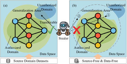
The primary challenge lies in the fact that the generalization region of well-trained models typically encompasses some unauthorized domains (as depicted in Fig. 1 (a)). It arises from the models’ innate ability to capture domain-invariant features, thereby leading to potential applicability IP infringements. An intuitive solution is to make the generalization bound of models more explicit and narrower, i.e., optimizing models to prioritize domain-dependent features and confining their applicability exclusively to authorized domains. To achieve this, NTL [49] first remolds the methodology in domain adaptation with an opposite objective. It amplifies the maximum mean difference (MMD) between the source (authorized) and target (unauthorized) domains, thereby effectively constraining the generalization scope of the models. Different from NTL, CUTI-domain [50] constructs middle domains with combined source and target features, which then act as barriers to block illegal transfers from authorized to unauthorized domains. Regardless of promising results, these methods require concurrent access to both source and target data when performing IP protection, rendering them unsuitable for decentralized private data scenarios. Moreover, they typically demand retraining from scratch to restrict the generalization boundary, which is highly inefficient since we may not have prior knowledge of all unauthorized data at the outset, leading to substantial resource waste.
In this paper, we target a practical but challenging setting where a well-trained source model is provided instead of source raw data, and investigate how we can realize source-free IP protection. To achieve this, we first introduce our Inverse Transfer Parameter Hypothesis inspired by the lottery ticket hypothesis [13]. We argue that well-trained models contain parameters exclusively associated with specific domains. Through deliberate pruning of these parameters, we effectively eliminate the generalization capability to these domains while minimizing the impact on other domains. To materialize this idea, we propose a novel MAsk Pruning (MAP) framework. MAP freezes the source model and learns a target-specific binary mask to prevent unauthorized data usage while minimizing performance degradation on authorized data. For a fair comparison, we first compare our MAP framework with existing methods when source data is available, denoted as SA-MAP. Subsequently, we evaluate MAP in source-free situations. Inspired by data-free knowledge distillation, we synthesize pseudo-source samples and amalgamate them with target data to train a target-specific mask for safeguarding the source model. This solution is denoted as SF-MAP. Moreover, we take a step further and explore a more challenging data-free setting, where both source and target data are unavailable. Building upon SF-MAP, we introduce a diversity generator for synthesizing auxiliary domains with diverse style features to mimic unavailable target data. We refer to this solution as DF-MAP. For performance evaluation, current methods only focus on performance drop on target (unauthorized) domain, but ignore the preservation of source domain performance. To address this, we introduce a new metric Source & Target Drop (ST-D) to fill this gap. We have conducted extensive experiments on several datasets, the results demonstrate the effectiveness of our MAP framework. The key contributions are summarized as follows:
-
•
To the best of our knowledge, we are the first to exploit and achieve source-free and data-free model IP protection settings. These settings consolidate the prevailing requirements for both model IP and data privacy protection.
-
•
We propose a novel and versatile MAsking Pruning (MAP) framework for model IP protection. MAP stems from our Inverse Transfer Parameter Hypothesis, i.e., well-trained models contain parameters exclusively associated with specific domains, pruning these parameters would assist us in model IP protection.
-
•
Extensive experiments on several datasets, ranging from source-available, source-free, to data-free settings, have verified and demonstrated the effectiveness of our MAP framework. Moreover, we introduce a new metric for thorough performance evaluation.
2 Related Work
Model Intellectual Property Protection. To gain improper benefits and collect private information in the model, some individuals have developed attack methods, such as the inference attack [2, 31, 55], model inversion attack [14, 58, 45], adversarial example attack [34, 56] and others [1, 33]. Therefore, the protection of model intellectual property rights has become important. Recent research has focused on ownership verification and usage authorization to preserve model intellectual property [49]. Traditional ownership verification methods [57, 25] employ watermarks to establish ownership by comparing results with and without watermarks. However, these techniques are also susceptible to certain watermark removal [17, 5] techniques. Usage authorization typically involves encrypting the entire or a portion of the network using a pre-set private key for access control purposes [38, 16].
As a usage authorization method, NTL [49] builds an estimator with the characteristic kernel from Reproduction Kernel Hilbert Spaces (RKHSs) to approximate the Maximum Mean Discrepancy (MMD) between two distributions to achieve the effect of reducing generalization to a certain domain. According to [50], CUTI-Domain generates a middle domain with source style and target semantic attributes to limit generalization region on both the middle and target domains. [48] enhances network performance by defining a divergence ball around the training distribution, covering neighboring distributions, and maximizing model risk on all domains except the training domain. However, the privacy protection policy results in difficulties in getting user source domain database data, which disables the above methods. To address this challenge, in this paper, we propose source-free and target-free model IP protection tasks.
Unstructured Parameter Pruning. Neural network pruning reduces redundant parameters in the model to alleviate storage pressure. It is done in two ways: unstructured or structured [19]. Structured pruning removes filters, while unstructured pruning removes partial weights, resulting in fine-grained sparsity. Unstructured pruning is more effective, but sparse tensor computations save runtime, and compressed sparse row forms add overhead [53].
There are several advanced methods for unstructure pruning. For example, [35] proposes a method that builds upon the concepts of network quantization and pruning, which enhances the network performance for a new task by utilizing binary masks that are either applied to unmodified weights on an existing network. As the basis of our hypothesis, the lottery hypothesis [13] illustrates that a randomly initialized, dense neural network has a sub-network that matches the test accuracy of the original network after at most the same number of iterations trained independently.
Source-Free Domain Adaptation. Domain adaptation addresses domain shifts by learning domain-invariant features between source and target domains [51]. In terms of source-free learning, our work is similar to source-free domain adaptation, which is getting more attention due to the data privacy policy [28]. [6] first considers prevention access to the source data in domain adaptation and then adjusts the source pre-trained classifier on all test data. Several approaches are used to apply the source classifier to unlabeled target domains [8, 46], and the current source-free adaptation paradigm does not exploit target labels by default [26, 29, 42]. Some schemes adopt the paradigm based on data generation [24, 39, 30], while others adopt the paradigm based on feature clustering [27, 26, 40, 41]. Our technique follows the former paradigm, which synthesizes a pseudo-source domain with prior information.
3 Methodology
In this paper, we designate the source domain as the authorized domain and the target domain as the unauthorized domain. Firstly, Section 3.1 defines the problem and our Inverse Transfer Parameter Hypothesis. Then Section 3.2, Section 3.3, and Section 3.4 present our MAsk-Pruning (MAP) framework in source-available, source-free, and data-free situations, respectively.
3.1 Problem Definition
Formally, we consider a source network trained on the source domain , a target network , and target domain . and are the distribution of and , respectively. The goal of source-available IP protection is to fine-tune while minimizing the generalization region of on target domain by using with and , in other words, degrade the performance of on while preserving its performance on [49, 50]. Due to increasingly stringent privacy protection policies, access to the or database of a user is more and more difficult [28]. Thus, we introduce IP protection for source-free and data-free scenarios. The objective of source-free model IP protection is to minimize the generalization region of a designated target domain by utilizing with . Data-free model IP protection is an extreme case. The objective is to minimize the generalization bound of by solely utilizing , without access to and .
To mitigate the risk of losing valuable knowledge stored in the model parameters, we initiate our approach with unstructured pruning of the model. The lottery ticket hypothesis, proposed by [13], is widely acknowledged as a fundamental concept in the field of model pruning. Building upon this foundation, we extend our Inverse Transfer Parameter Hypothesis as Hypothesis 1 in alignment with the principles presented in [13].
Hypothesis 1 (Inverse Transfer Parameter Hypothesis).
For a dense neural network well-trained on the source domain , there exists a sub-network like this: while achieves the same test accuracy as on , its performance significantly degrades on the target domain . The pruned parameters of relative to are crucial in determining its generalization capacity to .
3.2 Source-Avaliable Model IP Protection
To verify the soundness of Hypothesis 1, we first design the source-available MAsk Pruning (SA-MAP). has the same architecture as and is initialized with a well-trained checkpoint of . To maximize the risk of the target domain and minimize it in the source domain, we prune the ’s parameters by updating a binary mask of it and get a sub-network by optimizing the objective:
| (1) | |||
where presents the Kullback-Leibler divergence, and mean data and labels sampled from source domain and target domain , respectively. , and . and are the upper bound and scaling factor, respectively, which aim to limit the over-degradation of domain-invariant knowledge. We set and .
3.3 Source-Free Model IP Protection
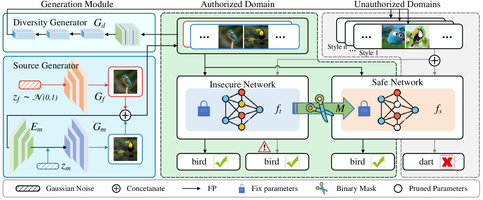
Under the source-free setting, we have no access to . To address this, we construct a replay-based source generator module to synthesize pseudo-source domain data . As illustrated in Fig. 2, SF-MAP is deformed by removing the Diversity Generator module and employing unlabeled target data.
Source generator module is composed of two generators to synthesize source feature samples, the fresh generator synthesizes samples with novel features, and the memory generator replays samples with origin features. Before sampling, we first train the fresh generator as Eq. (2). The objective of is to bring novel information to . To make synthesize the source-style samples, we leverage the loss function of Eq. (2). The first two items of Eq. (2) derive from [4], called predictive entropy and activation loss terms. These terms are designed to encourage the generator to produce high-valued activation maps and prediction vectors with low entropy, that is, to keep the generated samples consistent with the characteristics of the origin samples. As for the third item, denotes the Jensen-Shannon divergence, encouraging to obtain consistent results with .
| (2) |
where , and . means the generated novel sample by a gaussian noise , while . denotes the entropy of the class label distribution.
Along with the fresh generator , we optimize the memory generator and encoder as Eq. (3), which aims to replay the features from earlier distributions. To preserve the original features, we utilize the L1 distance to measure the similarity between the generated samples and reconstructed samples. The loss is defined as follows:
| (3) |
where means the L1 distance. is the selected layer set of . means reconstructed sample from the encoder-decoder structure. denotes the input synthetic sample concatenated by and . means memory sample, and .
After the generation process, we choose unlabeled target samples and synthetic source samples to train the target model based on Hypothesis 1, which is detailed in Algorithm 1. Adhering to the procedure in SA-MAP, we still employ the binary mask pruning strategy and update a of as follows:
| (4) | |||
where , , , , respectively. To improve pseudo labels , we utilize a set of data augmentation , when the prediction confidence conf() is lower than a threshold . and denote a scaling factor and an upper bound, respectively. We set and .
3.4 Data-Free Model IP Protection
When faced with challenging data-free situations, we adopt an exploratory approach to reduce the generalization region. Inspired by [52], we design a diversity generator with learnable mean shift and variance shift to extend the pseudo source samples to neighborhood domains of variant directions. The objective is to create as many neighboring domains as feasible to cover the most target domains and limit the generalization region. After generation, we concatenate samples with distinct directions as the whole pseudo auxiliary domain.
The latent vector of -th sample from the dataset is generated by the feature extractor of the source model , where means the classifier, and mean the dimension of latent space and class number, respectively. This component is designed to learn and capture potential features for the generator in a higher-dimensional feature space. Eq. (5) applies mutual information (MI) minimization to ensure variation between produced and original samples, ensuring distinct style features.
| (5) |
However, the semantic information between the same classes should be consistent. So we enhance the semantic consistency by minimizing the class-conditional maximum mean discrepancy (MMD) [44] in the latent space to enhance the semantic relation of the origin input sample and the generated sample in Eq. (6), and .
| (6) |
where and denote the latent vector of class of and . means an approximate distribution and means a kernel function. and are the number of origin and generated samples for class , respectively.
To generate diverse feature samples, we constrain different generation directions of the gradient for the generation process detailed in supplementary material. The optimization process follows the gradient because it is the most efficient way to reach the goal. In this case, all the generated domains will follow the same gradient direction [49]. So we restrict the gradient to get neighborhood domains with diverse directions. We split the generator network into parts. We limit direction by freezing the first parameters of convolutional layers. The gradient of the convolutional layer parameters is frozen during training, limiting the model’s learning capabilities in that direction.
4 Experiments
4.1 Implementation Details
Experiment Setup. Building upon existing works, we select representative benchmarks in transfer learning—the digit benchmarks (MNIST (MN) [11], USPS (US) [20], SVHN (SN) [36], MNIST-M (MM) [15]) and CIFAR10 [22], STL10 [9] VisDA-2017 [37] for object recognition. For IP protection task, we employ the VGG11 [43], VGG13 [43], and VGG19 [43] backbones, which is the same as [50]. The ablation study additionally evaluates on ResNet50 [18], ResNet101 [18], SwinT [32] and Xception [7] backbones. We mainly compare our MAP with the NTL [49] and CUTI [50] baselines. We leverage the unitive checkpoints trained on supervised learning (SL) to initialize. To fairly compare in the source-free scenario, we replace the source and target data with synthetic samples with the generator in Section 3.3 for all baselines. Experiments are performed on Python 3.8.16, PyTorch 1.7.1, CUDA 11.0, and NVIDIA GeForce RTX 3090 GPU. For each set of trials, we set the learning rate to 1e-4, and the batch size to 32.
Evaluation Metric. Existing works [49, 50] leverage the Source/Target Drop metric (), by quantifying the accuracy drop in the processed model compared to the original source model accuracy (), to verify the effectiveness. However, these two separate metrics make it difficult to evaluate the effectiveness of the method as a whole because performance degradation on illegal target domains has the risk of destroying source domain knowledge. In order to realize the trade-off, we propose ST-D as Eq. (7). A lower ST-D denotes enhanced IP protection, with a minimal drop on the source domain and a maximum on the target.
| (7) |
4.2 Result of MAP in Source-Available Situation
We first conduct experiments in the source-available situation to verify the effectiveness of our Hypothesis 1. As stated before,
we introduce the SA-MAP and optimize a binary mask to realize model IP protection and compare NTL, CUTI, and SA-MAP on digit datasets. Results in Table 1 show that SA-MAP achieves better Source Drop (-0.3%) and ST-D (-0.004), indicating the most deterioration in the target domain and the least in the source domain. It is noteworthy that SA-MAP even outperforms the origin model in the source domain (-0.3%). We speculate this may be the result of pruning, which removes redundant parameters.
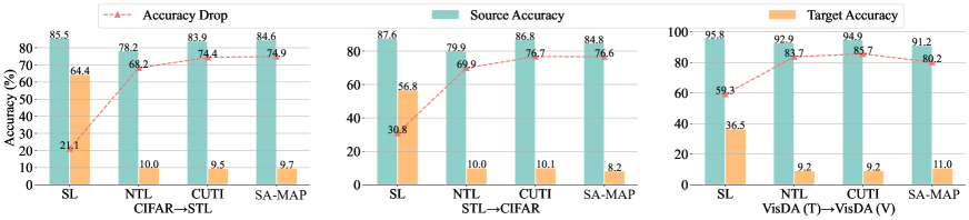
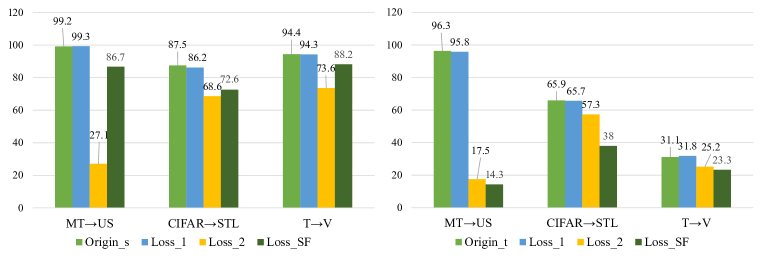
Fig. 3 assess method performance on CIFAR10, STL10, and VisDA-2017 benchmarks independently. We exploit VGG13 on CIFAR10STL10 experiment, and VGG19 on VisDA-2017 (TV). For a fair comparison, we utilize the same training recipe in [50].
A clear observation is that the pre-trained source model has good generalization performance on these three unauthorized tasks, seriously challenging the model IP. After performing protection, both baseline methods and our SA-MAP effectively reduce the performance on the target domain. SA-MAP achieves comparable or better results compared to baseline methods, which basically demonstrates our Hypothesis 1.
| Methods | Soure | Source Drop | Target Drop | ST-D |
|---|---|---|---|---|
| NTL [49] | MT | 1.5 (1.5%) | 50.9 (77.6%) | 0.019 |
| US | -0.2 (-0.2%) | 46.3 (84.0%) | -0.024 | |
| SN | 0.8 (0.9%) | 50.0 (85.2%) | 0.011 | |
| MM | 2.0 (2.1%) | 59.7 (79.2%) | 0.027 | |
| Mean | 1.0 (1.1%) | 51.7 (81.5%) | 0.013 | |
| CUTI [50] | MT | 0 (0%) | 52.7 (80.0%) | 0 |
| US | -0.1 (-0.1%) | 42.3 (78.6%) | -0.013 | |
| SN | 0.3 (0.3%) | 48.3 (82.3%) | 0.036 | |
| MM | 0.8 (0.8%) | 60.1 (80.0%) | 0.010 | |
| Mean | 0.3 (0.3%) | 50.9 (80.2%) | 0.004 | |
| SA-MAP (ours) | MT | -0.1 (-0.1%) | 51.0 (77.8%) | -0.013 |
| US | 0 (0%) | 45.2 (82.1%) | 0 | |
| SN | -0.8 (-0.9%) | 49.6 (84.4%) | -0.012 | |
| MM | -0.1 (-0.1%) | 60.4 (80.2%) | -0.012 | |
| Mean | -0.3 (-0.3%) | 51.6 (81.1%) | -0.004 |
4.3 Result of MAP in Source-Free Situation
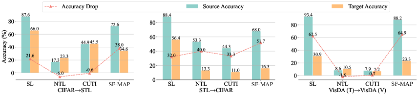
We then perform model IP protection in the challenging source-free situation and present our SF-MAP solution. We train NTL, CUTI, and SF-MAP with the same samples from Section 3.3 for fairness. Table 2 illustrates a considerable source drop of NTL (68.9%) and CUTI (87.4%) lead to 1.01 and 1.08 ST-D, respectively. While SF-MAP achieves better Source Drop (8.8%) and ST-D (0.24). The backbone in Fig. 4 is configured to correspond with the experimental setup described in Section 4.2. In particular, SF-MAP exhibits higher performance with relative degradations of 38.0%, 51.7%, and 64.9%, respectively.
We attribute impressive results to the binary mask pruning strategy. Arbitrary scaling of network parameters using continuous masks or direct adjustments has the potential to catastrophic forgetting. Precisely eliminating parameters through a binary mask offers a more effective and elegant solution for IP protection, while concurrently preventing the loss of the network’s existing knowledge.
| Methods | Source/Target | MT | US | SN | MM | Source Drop | Target Drop | ST-D |
|---|---|---|---|---|---|---|---|---|
| NTL [49] | MT | 98.9 / 41.3 | 96.3 / 38.9 | 36.3 / 19.0 | 64.9 / 11.1 | 57.6 (58.2%) | 49.5 (65.1%) | 0.89 |
| US | 90.0 / 33.2 | 99.7 / 40.0 | 32.8 / 6.8 | 42.4 / 10.8 | 59.7 (59.9%) | 38.1 (69.2%) | 0.86 | |
| SN | 68.2 / 20.5 | 75.0 / 32.7 | 92.0 / 19.4 | 32.8 / 9.2 | 72.6 (78.9%) | 37.9 (64.5%) | 1.22 | |
| MM | 97.5 / 11.3 | 88.3 / 30.7 | 40.2 / 19.0 | 96.8 / 20.6 | 76.2 (78.7%) | 55.0 (73.0%) | 1.08 | |
| Mean | / | / | / | / | 66.5 (68.9%) | 45.1 (68.0%) | 1.01 | |
| CUTI [50] | MT | 98.9 / 13.0 | 96.3 / 14.1 | 36.3 / 19.0 | 64.9 / 11.2 | 85.9 (86.9%) | 51.1 (77.5%) | 1.12 |
| US | 90.0 / 10.7 | 99.7 / 7.8 | 32.8 / 6.6 | 42.4 / 10.6 | 91.9 (92.2%) | 53.1 (83.1%) | 1.11 | |
| SN | 68.2 / 9.3 | 75.0 / 14.1 | 92.0 / 13.6 | 32.8 / 9.4 | 78.4 (85.2%) | 47.7 (81.4%) | 1.05 | |
| MM | 97.5 / 11.4 | 88.3 / 14.1 | 40.2 / 19.0 | 96.8 / 14.2 | 82.6 (85.3%) | 60.5 (80.3%) | 1.06 | |
| Mean | / | / | / | / | 84.7 (87.4%) | 53.1 (80.6%) | 1.08 | |
| SF-MAP (ours) | MT | 99.2 / 90.2 | 96.3 / 59.9 | 36.7 / 19.4 | 64.8 / 24.5 | 9.0 (9.0%) | 31.3 (47.5%) | 0.19 |
| US | 90.0 / 67.3 | 99.7 / 83.5 | 32.8 / 7.1 | 42.4 / 30.8 | 16.2 (16.2%) | 20.0 (36.3%) | 0.45 | |
| SN | 68.2 / 34.8 | 75.0 / 52.5 | 91.4 / 87.2 | 32.8 / 32.0 | 4.2 (4.6%) | 25.0 (32.2%) | 0.12 | |
| MM | 97.6 / 93.3 | 88.5 / 49.0 | 40.2 / 22.1 | 97.0 / 91.8 | 5.2 (5.4%) | 19.6 (27.4%) | 0.20 | |
| Mean | / | / | / | / | 8.7 (8.8%) | 24.0 (35.9%) | 0.24 |
| Methods | Source/Target | MT | US | SN | MM | Source Drop | Target Drop | ST-D |
|---|---|---|---|---|---|---|---|---|
| DF-MAP (ours) | MT | 99.1 / 95.0 | 96.8 / 72.0 | 37.1 / 15.1 | 67.5 / 14.7 | 4.1 (4.1%) | 33.2 (37.8%) | 0.11 |
| US | 89.4 / 83.8 | 99.8 / 99.5 | 34.9 / 31.0 | 33.8 / 16.8 | 0.3 (0.3%) | 8.8 (10.3%) | 0.03 | |
| SN | 58.6 / 46.6 | 70.9 / 59.2 | 91.5 / 76.3 | 29.5 / 24.2 | 15.2 (16.6%) | 9.7 (18.2%) | 0.91 | |
| MM | 98.8 / 94.8 | 84.4 / 61.3 | 40.2 / 28.8 | 96.5 / 94.7 | 1.8 (1.9%) | 12.8 (17.2%) | 0.11 | |
| Mean | / | / | / | / | 5.4 (5.7%) | 16.1 (20.9%) | 0.27 |
| Source | Avg Drop | |||
|---|---|---|---|---|
| SL | NTL | CUTI | MAP | |
| MT | 0.2 | 87.9 | 87.7 | 88.6 |
| US | 0.1 | 85.7 | 93.0 | 92.5 |
| SN | -0.8 | 66.4 | 46.9 | 47.5 |
| MM | 4.4 | 83.9 | 79.6 | 79.2 |
| CIFAR | 0 | 27.4 | 38.4 | 56.2 |
| STL | -6.7 | 54.8 | 62.0 | 60.1 |
| VisDA | 0.1 | 0.1 | 22.4 | 19.1 |
| Mean | -0.3 | 58.0 | 61.4 | 63.3 |
4.4 Result of MAP in Data-Free Situation
We next present our DF-MAP in the extremely challenging data-free setting. Section 4.3 indicates that the current techniques are not suited to source-free scenarios. Due to the absence of relevant research to our best knowledge, we refrain from specifying or constructing the baseline in the data-free situation. Table 3 indicates DF-MAP achieved IP protection by achieving a lower decrease in source domains and a higher drop in target domains, as illustrated by ST-D being less than 1.0 for all sets of experiments.
4.5 Result of Ownership Verification
After the above, we additionally conduct an ownership verification experiment of MAP using digit datasets and VGG11 backbone. Following existing work [49], we apply a watermark to source domain samples, treating it as an unauthorized auxiliary domain. As shown in Table 4, MAP performed 1.9% better than the second, which demonstrates the utility of this model IP protection approach.
4.6 Ablation Study
Backbone. To verify the generality of MAP for different network architectures, we examine it for several backbones, including VGG11, VGG13, VGG19 [43], ResNet18, ResNet34 [18], Swin-Transformer [32], and Xception [7]. Experiments are conducted on STL10 CIFAR10. We evaluate model accuracy on the target domain with minimal source domain influence. Fig. 5 (a) illustrates that SF-MAP achieves consistently lower accuracy in unauthorized target domains than the origin model in supervised learning, demonstrating its universality for different backbones.
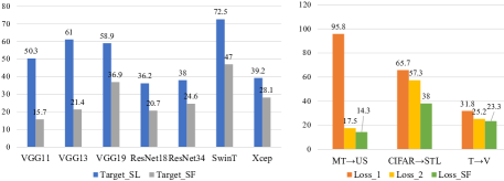
Loss Function. Eq. (4) suggests shaped as , where and . We conduct ablation studies to verify each loss component’s contribution. We utilize , , and to train SF-MAP on MNUS, CIFAR10STL10, and VisDA-2017 (TV). According to Fig. 5 (b), the result on has the minimum drop to the target domain due to poor simulation of its features. The result on shows the greatest target drop without affecting the source domain, but significantly degrades source performance, as detailed in the supplementary. The is more accurate than in recognizing domain-invariant characteristics, eliminating redundant parameters, and degrading the target domain performance.
Visualization. Fig. 6 (a) illustrates the MNUS experiment convergence analysis diagram. With SF-MAP, source, and target domain model performance is more balanced. The fact that NTL changes all model parameters may lead to forgetting the source feature and inferior results. In the absence of the real source domain, CUTI’s middle domain may aggravate forgetting origin source features since synthesized source domains may have unobserved style features. Fig. 6 (b) illustrates the T-SNE figures of MNMM. The origin supervised learning (SL) model, NTL, CUTI, and SF-MAP results are exhibited with the source domain MNIST in blue and the target domain MNISTM in red. As illustrated in Fig. 6 (b), SF-MAP’s source domain data retains better clustering information than other approaches, while the target domain is corrupted.

5 Conclusion
Attacks on neural networks have led to a great need for model IP protection. To address the challenge, we present MAP, a mask-pruning-based model IP protection method stemming from our Inverse Transfer Parameter Hypothesis, and its expansion forms (SA-MAP, SF-MAP, and DF-MAP) under source-available, source-free, and data-free conditions. SA-MAP updates a learnable binary mask to prune target-related parameters. Based on SA-MAP, SF-MAP uses replay-based generation to synthesize pseudo source samples. We further suggest a diversity generator in DF-MAP to construct neighborhood domains with unique styles. To trade off source and target domains’ evaluation, the ST-D metric is proposed. Experiments conducted on digit datasets, CIFAR10, STL10, and VisDA, demonstrate that MAP significantly diminishes model generalization region in source-available, source-free, and data-free situations, while still maintaining source domain performance, ensuring the effectiveness of model IP protection.
Acknowledgment: This work is supported by the National Natural Science Foundation of China (No.62372329), in part by the National Key Research and Development Program of China (No.2021YFB2501104), in part by Shanghai Rising Star Program (No.21QC1400900), in part by Tongji-Qomolo Autonomous Driving Commercial Vehicle Joint Lab Project, and Xiaomi Young Talents Program.
Supplementary Material
Appendix A Theoretical Analysis
Formally, we consider a source network trained on source domain , a target network , and target domain . and are the distribution of and , respectively. The goal of IP protection is to fine-tune while minimizing the generalization region of on target domain , in other words, degrade the performance of on unauthorized target domain while preserving performance on authorized source .
A.1 Definitions
Proposition 1 ([49]).
Let be a nuisance for input . Let be a representation of , and the label is . The Shannon Mutual Information (SMI) is presented as . For the information flow in representation learning, we have
| (8) |
Lemma 1 ([49]).
Let be the predicted label outputted by a representation model when feeding with input , and suppose that is a scalar random variable and is balanced on the ground truth label . And is the distribution. If the KL divergence loss increases, the mutual information will decrease.
A.2 Details of Optimization Objective Design
In the context of intellectual property (IP) protection, the objective is to maximize on the unauthorized domain, and Proposition 8 provides guidance by aiming to minimize . According to Lemma 1, if the Kullback-Leibler (KL) divergence loss increases, the mutual information will decrease. Since , the will consistently decrease with . Please note that Proposition 8 and Lemma 1 have been proved in [49]. Therefore, the in Eq. 9, , and in the main paper are designed in the form of , where and . This design allows us to maximize on the unauthorized (target) domain and minimize on the authorized (source) domain.

Appendix B Details of MAP Architecture
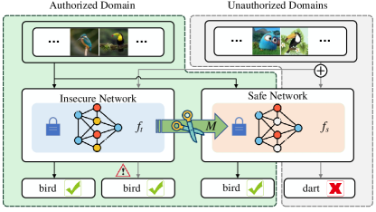
As elaborated in the main text, we present the comprehensive architectural depiction of DF-MAP. In this supplementary, Fig. 7 and Fig. 8 showcase the exhaustive architectures of SA-MAP and SF-MAP, respectively. In the source-available scenario, access is available to labeled source samples and target samples . We designate the source domain as the authorized domain, anticipating good performance, and the target domain as the unauthorized domain, expecting the opposite. As depicted in Fig. 7, the classification example illustrates that the secure network should correctly classify results on the authorized domain while producing erroneous results on unauthorized ones. We iteratively update a binary mask for the insecure model to prune redundant parameters, which contributes to the generalization to unauthorized domains.
In the preceding discussion, represents the target network, and represents the source network, both sharing the same architecture and well-trained weight initialization. In the right part of Fig. 7, the pruned source network can be regarded as a sub-network, aligning with our Inverse Transfer Parameter Hypothesis outlined in the main paper. More precisely, we gradually update to prune redundant target-featured parameters of , enabling the pruned to progressively approximate the sub-network of . The complete source network is employed in the Generation Module in Fig. 8 to generate the source-style samples.
We further explore the SF-MAP architecture for the source-free model IP protection task, as illustrated in Fig. 8. In the source-free scenario, access is limited to unlabeled target samples and the well-trained weights () of trained on the source domain . Consequently, we generate pseudo source domain samples and pseudo labels for the target domain, as aforementioned. Please note that we are trying to improve the quality of , rather than creating a uniform distribution label space for the target domain. Because we want to precisely increase on the target domain, the latter will have a negative influence on the feature on other domains or even the source domain. Overall, the and Generation Module in Fig. 8 play a pivotal component within SF-MAP, particularly considering the challenge of synthesizing source-featured samples with only and .
Appendix C Details of Experiments
C.1 Details of Datasets
We implemented our methods and baseline on seven popular benchmarks widely used in domain adaptation and domain generalization. The digit benchmarks include MNIST [11], USPS [20], SVHN [36], and MNIST-M [15]. These benchmarks aim to classify each digit into one of ten classes (0-9). MNIST consists of 28x28 pixel grayscale images of handwritten digits, with a training set of 60,000 examples and a test set of 10,000 examples. USPS is a dataset scanned from envelopes, comprising 9,298 16x16 pixel grayscale samples. SVHN contains 600,000 32x32 RGB images of printed digits cropped from pictures of house number plates. MNIST-M is created by combining the MNIST with randomly drawn color photos from the BSDS500 [54] dataset as a background, consisting of 59,001 training images and 90,001 test images.
Additionally, we employed CIFAR10 [22], STL10 [9], and VisDA2017 [37] for image classification tasks. CIFAR10 is a subset of the Tiny Images dataset, featuring 60,000 32x32 color images with 10 object classes. STL-10 is an image dataset processed from ImageNet, comprising 13,000 96x96 pixel RGB images with 10 object classes. VisDA2017 is a simulation-to-real dataset for domain adaptation, containing 12 categories and over 280,000 images.
C.2 Details of SA-MAP result
Due to space constraints in the main paper, only a portion of the SA-MAP results are presented. In this supplementary section, we provide the detailed results in Table 5. The detailed version primarily includes the drop rate for each experiment group. The results of MAP in the source-available setting exhibit better performance. The true advantage of SA-MAP lies in the elimination of the need for retraining from scratch. The obtained sub-network effectively demonstrates our Inverse Transfer Parameter Hypothesis.
| Model | Source/Target | MT | US | SN | MM | Source Drop | Target Drop | ST-D |
|---|---|---|---|---|---|---|---|---|
| NTL | MT | 98.9 / 97.4 | 96.3 / 14.0 | 36.3 / 19.0 | 64.9 / 11.2 | 1.5 (1.5%) | 50.9 (77.6%) | 0.019 |
| US | 90.0 / 10.8 | 99.7 / 99.9 | 32.8 / 7.1 | 42.5 / 8.5 | -0.2 (-0.2%) | 46.3 (84.0%) | -0.024 | |
| SN | 68.4 / 9.0 | 74.9 / 8.1 | 91.9 / 91.1 | 32.8 / 9.0 | 0.8 (0.9%) | 50.0 (85.2%) | 0.011 | |
| MM | 97.6 / 11.3 | 88.2 / 16.4 | 40.1 / 19.2 | 96.8 / 95.1 | 2.0 (2.1%) | 59.7 (79.2%) | 0.027 | |
| Mean | / | / | / | / | 1.0 (1.1%) | 51.7 (81.5%) | 0.013 | |
| CUTI | MT | 98.9 / 98.9 | 96.3 / 7.8 | 36.3 / 19.1 | 64.9 / 12.7 | 0 (0%) | 52.7 (80.0%) | 0 |
| US | 90.0 / 16.7 | 99.7 / 99.8 | 32.8 / 10.1 | 42.5 / 8.5 | -0.1 (-0.1%) | 42.3 (78.6%) | -0.013 | |
| SN | 68.4 / 9.3 | 74.9 / 12.6 | 91.9 / 91.6 | 32.8 / 9.2 | 0.3 (0.3%) | 48.3 (82.3%) | 0.036 | |
| MM | 97.6 / 11.6 | 88.2 / 14.1 | 40.1 / 19.8 | 97.1/96.3 | 0.8 (0.8%) | 60.1 (80.0%) | 0.010 | |
| Mean | / | / | / | / | 0.3 (0.3%) | 50.9 (80.2%) | 0.004 | |
| MAP (ours) | MT | 98.9 / 99.0 | 96.3 / 14.3 | 36.3 / 18.9 | 64.9 / 10.7 | -0.1 (-0.1%) | 51.0 (77.8%) | -0.013 |
| US | 90.0 / 11.0 | 99.7 / 99.7 | 32.8 / 7.8 | 42.5 / 10.8 | 0 (0%) | 45.2 (82.1%) | 0 | |
| SN | 68.4 / 9.5 | 74.9 / 8.5 | 91.9 / 92.7 | 32.8 / 9.4 | -0.8 (-0.9%) | 49.6 (84.4%) | -0.012 | |
| MM | 97.6 / 11.2 | 88.2 / 14.3 | 40.1 / 19.3 | 97.1 / 97.2 | -0.1 (-0.1%) | 60.4 (80.2%) | -0.012 | |
| Mean | / | / | / | / | -0.3 (-0.3%) | 51.6 (81.1%) | -0.004 |
| Source | Methods | Avg Drop | ||||||
|---|---|---|---|---|---|---|---|---|
| SL | NTL | CUTI | MAP | SL | NTL | CUTI | MAP | |
| MT | 99.2 / 99.4 | 11.2 / 99.1 | 11.4 / 99.1 | 9.7 / 98.3 | 0.2 | 87.9 | 87.7 | 88.6 |
| US | 99.5 / 99.6 | 14.0 / 99.7 | 6.8 / 99.8 | 6.8 / 99.3 | 0.1 | 85.7 | 93.0 | 92.5 |
| SN | 91.1 / 90.3 | 24.0 / 90.4 | 43.5 / 90.4 | 34.8 / 82.3 | -0.8 | 66.4 | 46.9 | 47.5 |
| MM | 92.1 / 96.5 | 12.8 / 96.7 | 17.1 / 96.7 | 16.7 / 95.9 | 4.4 | 83.9 | 79.6 | 79.2 |
| CIFAR | 85.7 / 85.7 | 56.8 / 84.2 | 45.3 / 83.7 | 23.5 / 79.7 | 0 | 27.4 | 38.4 | 56.2 |
| STL | 93.2 / 86.5 | 26.4 / 81.2 | 22.7 / 84.7 | 22.1 / 82.2 | -6.7 | 54.8 | 62.0 | 60.1 |
| VisDA | 92.4 / 92.5 | 93.1 / 93.2 | 73.8 / 92.9 | 70.6 / 89.7 | 0.1 | 0.1 | 22.4 | 19.1 |
| Mean | / | / | / | / | -0.3 | 58.0 | 61.4 | 63.3 |
C.3 Details of Data-Free Model IP Protection
We provide the Algorithm 2 of Section 3.4 in the main paper. The optimization procedure adheres to the gradient as it represents the most effective path towards achieving the specified objective. In this particular instance, all produced domains exhibit alignment with a consistent gradient direction [49]. To introduce diversity in directional perspectives within the generated domains, we impose constraints on the gradient. Specifically, we decompose the generator network into segments. To restrict the direction indexed by , we employ a freezing strategy by fixing the initial parameters of convolutional layers. This approach entails the immobilization of the gradient with respect to the convolutional layer parameters during training, thereby constraining the model’s learning capacity along that particular direction.
C.4 Details of Ownership Verification
We adopt the method from [49] to introduce a model watermark to the source domain data, creating a new auxiliary domain . In this experiment, we utilize the watermarked auxiliary samples as the unauthorized samples, exhibiting poor performance when evaluated by model . The original source samples without watermarks represent the authorized samples, intended to yield good performance. The details of the ownership verification experiments are outlined in Algorithm 3.
| (9) | |||
where presents the Kullback-Leibler divergence. and mean the prediction of target model . means a scaling factor and means an upper bound. We set and
The detailed results in Table 6 reveal that the original model in supervised learning (SL) struggles to differentiate between the source domain and the watermarked authorized domain , achieving similar results on both. In contrast, established model intellectual property (IP) protection methods such as NTL [49], CUTI [50], and our SA-MAP exhibit distinct advantages. These methods showcase superior performance on compared to . Particularly noteworthy is the performance of SA-MAP, which outperforms the other methods, showcasing a 1.9% improvement over the second-best approach.
C.5 Details of Ablation Study
The detailed ablation figure, highlighting various loss functions, is depicted in Fig. 9. As stated before, the model trained with demonstrates superior performance on both the source and target domains. In the case of , the outcome closely resembles that of the original model, indicating a lack of effective model intellectual property (IP) protection. On the other hand, with , although there is a reduction in accuracy on the target domain, there is a noteworthy decline on the source domain, signifying a failure to adequately preserve the source performance.
References
- Binici et al. [2022] Kuluhan Binici, Shivam Aggarwal, Nam Trung Pham, Karianto Leman, and Tulika Mitra. Robust and resource-efficient data-free knowledge distillation by generative pseudo replay. In AAAI, 2022.
- Carlini et al. [2022] Nicholas Carlini, Steve Chien, Milad Nasr, Shuang Song, Andreas Terzis, and Florian Tramer. Membership inference attacks from first principles. In 2022 IEEE Symposium on Security and Privacy (SP), pages 1897–1914. IEEE, 2022.
- Charette et al. [2022] Laurent Charette, Lingyang Chu, Yizhou Chen, Jian Pei, Lanjun Wang, and Yong Zhang. Cosine model watermarking against ensemble distillation. In AAAI, 2022.
- Chen et al. [2019] Hanting Chen, Yunhe Wang, Chang Xu, Zhaohui Yang, Chuanjian Liu, Boxin Shi, Chunjing Xu, Chao Xu, and Qi Tian. Data-free learning of student networks. In ICCV, 2019.
- Chen et al. [2021] Xinyun Chen, Wenxiao Wang, Chris Bender, Yiming Ding, Ruoxi Jia, Bo Li, and Dawn Song. Refit: a unified watermark removal framework for deep learning systems with limited data. In Proceedings of the 2021 ACM Asia Conference on Computer and Communications Security, pages 321–335, 2021.
- Chidlovskii et al. [2016] Boris Chidlovskii, Stephane Clinchant, and Gabriela Csurka. Domain adaptation in the absence of source domain data. In Proceedings of the 22nd ACM SIGKDD International Conference on Knowledge Discovery and Data Mining, pages 451–460, 2016.
- Chollet [2017] François Chollet. Xception: Deep learning with depthwise separable convolutions. In CVPR, 2017.
- Clinchant et al. [2016] Stéphane Clinchant, Boris Chidlovskii, and Gabriela Csurka. Transductive adaptation of black box predictions. In Proceedings of the 54th Annual Meeting of the Association for Computational Linguistics (Volume 2: Short Papers), pages 326–331, 2016.
- Coates et al. [2011] Adam Coates, Andrew Ng, and Honglak Lee. An analysis of single-layer networks in unsupervised feature learning. In Proceedings of the fourteenth international conference on artificial intelligence and statistics, pages 215–223. JMLR Workshop and Conference Proceedings, 2011.
- Deng et al. [2009] Jia Deng, Wei Dong, Richard Socher, Li-Jia Li, Kai Li, and Li Fei-Fei. Imagenet: A large-scale hierarchical image database. In CVPR, 2009.
- Deng [2012] Li Deng. The mnist database of handwritten digit images for machine learning research [best of the web]. IEEE signal processing magazine, 29(6):141–142, 2012.
- Dosovitskiy et al. [2021] Alexey Dosovitskiy, Lucas Beyer, Alexander Kolesnikov, Dirk Weissenborn, Xiaohua Zhai, Thomas Unterthiner, Mostafa Dehghani, Matthias Minderer, Georg Heigold, Sylvain Gelly, et al. An image is worth 16x16 words: Transformers for image recognition at scale. In ICLR, 2021.
- Frankle and Carbin [2018] Jonathan Frankle and Michael Carbin. The lottery ticket hypothesis: Finding sparse, trainable neural networks. arXiv preprint arXiv:1803.03635, 2018.
- Fredrikson et al. [2015] Matt Fredrikson, Somesh Jha, and Thomas Ristenpart. Model inversion attacks that exploit confidence information and basic countermeasures. In Proceedings of the 22nd ACM SIGSAC conference on computer and communications security, pages 1322–1333, 2015.
- Ganin et al. [2016] Yaroslav Ganin, Evgeniya Ustinova, Hana Ajakan, Pascal Germain, Hugo Larochelle, François Laviolette, Mario Marchand, and Victor Lempitsky. Domain-adversarial training of neural networks. JMLR, 2016.
- Guan et al. [2022] Jiyang Guan, Jian Liang, and Ran He. Are you stealing my model? sample correlation for fingerprinting deep neural networks. NeurIPS, 2022.
- Guo et al. [2020] Shangwei Guo, Tianwei Zhang, Han Qiu, Yi Zeng, Tao Xiang, and Yang Liu. Fine-tuning is not enough: A simple yet effective watermark removal attack for dnn models. arXiv preprint arXiv:2009.08697, 2020.
- He et al. [2016] Kaiming He, Xiangyu Zhang, Shaoqing Ren, and Jian Sun. Deep residual learning for image recognition. In CVPR, 2016.
- He and Xiao [2023] Yang He and Lingao Xiao. Structured pruning for deep convolutional neural networks: A survey. arXiv preprint arXiv:2303.00566, 2023.
- Hull [1994] Jonathan J. Hull. A database for handwritten text recognition research. IEEE TPAMI, 16(5):550–554, 1994.
- Kirillov et al. [2023] Alexander Kirillov, Eric Mintun, Nikhila Ravi, Hanzi Mao, Chloe Rolland, Laura Gustafson, Tete Xiao, Spencer Whitehead, Alexander C Berg, Wan-Yen Lo, et al. Segment anything. In ICCV, 2023.
- Krizhevsky et al. [2009] Alex Krizhevsky, Geoffrey Hinton, et al. Learning multiple layers of features from tiny images. 2009.
- Li et al. [2023] Peixuan Li, Pengzhou Cheng, Fangqi Li, Wei Du, Haodong Zhao, and Gongshen Liu. Plmmark: a secure and robust black-box watermarking framework for pre-trained language models. In AAAI, 2023.
- Li et al. [2020] Rui Li, Qianfen Jiao, Wenming Cao, Hau-San Wong, and Si Wu. Model adaptation: Unsupervised domain adaptation without source data. In CVPR, 2020.
- Li et al. [2019] Zheng Li, Chengyu Hu, Yang Zhang, and Shanqing Guo. How to prove your model belongs to you: A blind-watermark based framework to protect intellectual property of dnn. In Proceedings of the 35th Annual Computer Security Applications Conference, pages 126–137, 2019.
- Liang et al. [2020] Jian Liang, Dapeng Hu, and Jiashi Feng. Do we really need to access the source data? source hypothesis transfer for unsupervised domain adaptation. In ICML. PMLR, 2020.
- Liang et al. [2021] Jian Liang, Dapeng Hu, Yunbo Wang, Ran He, and Jiashi Feng. Source data-absent unsupervised domain adaptation through hypothesis transfer and labeling transfer. IEEE TPAMI, 44(11):8602–8617, 2021.
- Liang et al. [2023] Jian Liang, Ran He, and Tieniu Tan. A comprehensive survey on test-time adaptation under distribution shifts. arXiv preprint arXiv:2303.15361, 2023.
- Liu et al. [2021a] Yuejiang Liu, Parth Kothari, Bastien Van Delft, Baptiste Bellot-Gurlet, Taylor Mordan, and Alexandre Alahi. Ttt++: When does self-supervised test-time training fail or thrive? NeurIPS, 2021a.
- Liu et al. [2021b] Yuang Liu, Wei Zhang, and Jun Wang. Source-free domain adaptation for semantic segmentation. In CVPR, 2021b.
- Liu et al. [2022] Yiyong Liu, Zhengyu Zhao, Michael Backes, and Yang Zhang. Membership inference attacks by exploiting loss trajectory. In Proceedings of the 2022 ACM SIGSAC Conference on Computer and Communications Security, pages 2085–2098, 2022.
- Liu et al. [2021c] Ze Liu, Yutong Lin, Yue Cao, Han Hu, Yixuan Wei, Zheng Zhang, Stephen Lin, and Baining Guo. Swin transformer: Hierarchical vision transformer using shifted windows. In ICCV, 2021c.
- Lopes et al. [2017] Raphael Gontijo Lopes, Stefano Fenu, and Thad Starner. Data-free knowledge distillation for deep neural networks. arXiv preprint arXiv:1710.07535, 2017.
- Luo et al. [2018] Bo Luo, Yannan Liu, Lingxiao Wei, and Qiang Xu. Towards imperceptible and robust adversarial example attacks against neural networks. In AAAI, 2018.
- Mallya et al. [2018] Arun Mallya, Dillon Davis, and Svetlana Lazebnik. Piggyback: Adapting a single network to multiple tasks by learning to mask weights. In ECCV, 2018.
- Netzer et al. [2011] Yuval Netzer, Tao Wang, Adam Coates, Alessandro Bissacco, Bo Wu, and Andrew Y Ng. Reading digits in natural images with unsupervised feature learning. In NeurIPS Workshop on Deep Learning and Unsupervised Feature Learning, 2011.
- Peng et al. [2017] Xingchao Peng, Ben Usman, Neela Kaushik, Judy Hoffman, Dequan Wang, and Kate Saenko. Visda: The visual domain adaptation challenge. arXiv preprint arXiv:1710.06924, 2017.
- Peng et al. [2022] Zirui Peng, Shaofeng Li, Guoxing Chen, Cheng Zhang, Haojin Zhu, and Minhui Xue. Fingerprinting deep neural networks globally via universal adversarial perturbations. In CVPR, 2022.
- Qiu et al. [2021] Zhen Qiu, Yifan Zhang, Hongbin Lin, Shuaicheng Niu, Yanxia Liu, Qing Du, and Mingkui Tan. Source-free domain adaptation via avatar prototype generation and adaptation. arXiv preprint arXiv:2106.15326, 2021.
- Qu et al. [2022] Sanqing Qu, Guang Chen, Jing Zhang, Zhijun Li, Wei He, and Dacheng Tao. Bmd: A general class-balanced multicentric dynamic prototype strategy for source-free domain adaptation. In ECCV, 2022.
- Qu et al. [2023] Sanqing Qu, Tianpei Zou, Florian Röhrbein, Cewu Lu, Guang Chen, Dacheng Tao, and Changjun Jiang. Upcycling models under domain and category shift. In CVPR, 2023.
- Qu et al. [2024] Sanqing Qu, Tianpei Zou, Lianghua He, Florian Röhrbein, Alois Knoll, Guang Chen, and Changjun Jiang. Lead: Learning decomposition for source-free universal domain adaptation. In CVPR, 2024.
- Simonyan and Zisserman [2014] Karen Simonyan and Andrew Zisserman. Very deep convolutional networks for large-scale image recognition. arXiv preprint arXiv:1409.1556, 2014.
- Sriperumbudur et al. [2010] Bharath K Sriperumbudur, Arthur Gretton, Kenji Fukumizu, Bernhard Schölkopf, and Gert RG Lanckriet. Hilbert space embeddings and metrics on probability measures. JMLR, 2010.
- Struppek et al. [2022] Lukas Struppek, Dominik Hintersdorf, Antonio De Almeida Correia, Antonia Adler, and Kristian Kersting. Plug & play attacks: Towards robust and flexible model inversion attacks. arXiv preprint arXiv:2201.12179, 2022.
- van Laarhoven and Marchiori [2017] Twan van Laarhoven and Elena Marchiori. Unsupervised domain adaptation with random walks on target labelings. arXiv preprint arXiv:1706.05335, 2017.
- Vybornova and Ulyanov [2022] YD Vybornova and DI Ulyanov. Method for protection of deep learning models using digital watermarking. In 2022 VIII International Conference on Information Technology and Nanotechnology (ITNT), pages 1–5. IEEE, 2022.
- Wang et al. [2023a] Haotian Wang, Haoang Chi, Wenjing Yang, Zhipeng Lin, Mingyang Geng, Long Lan, Jing Zhang, and Dacheng Tao. Domain specified optimization for deployment authorization. In ICCV, pages 5095–5105, 2023a.
- Wang et al. [2021a] Lixu Wang, Shichao Xu, Ruiqi Xu, Xiao Wang, and Qi Zhu. Non-transferable learning: A new approach for model ownership verification and applicability authorization. arXiv preprint arXiv:2106.06916, 2021a.
- Wang et al. [2023b] Lianyu Wang, Meng Wang, Daoqiang Zhang, and Huazhu Fu. Model barrier: A compact un-transferable isolation domain for model intellectual property protection. In CVPR, 2023b.
- Wang and Deng [2018] Mei Wang and Weihong Deng. Deep visual domain adaptation: A survey. Neurocomputing, 312:135–153, 2018.
- Wang et al. [2021b] Zijian Wang, Yadan Luo, Ruihong Qiu, Zi Huang, and Mahsa Baktashmotlagh. Learning to diversify for single domain generalization. In ICCV, 2021b.
- Wimmer et al. [2022] Paul Wimmer, Jens Mehnert, and Alexandru Condurache. Interspace pruning: Using adaptive filter representations to improve training of sparse cnns. In CVPR, 2022.
- Yang et al. [2016] Jimei Yang, Brian Price, Scott Cohen, Honglak Lee, and Ming-Hsuan Yang. Object contour detection with a fully convolutional encoder-decoder network. In CVPR, 2016.
- Ye et al. [2022] Jiayuan Ye, Aadyaa Maddi, Sasi Kumar Murakonda, Vincent Bindschaedler, and Reza Shokri. Enhanced membership inference attacks against machine learning models. In Proceedings of the 2022 ACM SIGSAC Conference on Computer and Communications Security, pages 3093–3106, 2022.
- Yuan et al. [2021] Chaoran Yuan, Xiaobin Liu, and Zhengyuan Zhang. The current status and progress of adversarial examples attacks. In 2021 International Conference on Communications, Information System and Computer Engineering (CISCE), pages 707–711. IEEE, 2021.
- Zhang et al. [2018] Jialong Zhang, Zhongshu Gu, Jiyong Jang, Hui Wu, Marc Ph Stoecklin, Heqing Huang, and Ian Molloy. Protecting intellectual property of deep neural networks with watermarking. In Proceedings of the 2018 on Asia conference on computer and communications security, pages 159–172, 2018.
- Zhang et al. [2022] Zaixi Zhang, Qi Liu, Zhenya Huang, Hao Wang, Chee-Kong Lee, and Enhong Chen. Model inversion attacks against graph neural networks. IEEE TKDE, 2022.
- Zoph and Le [2016] Barret Zoph and Quoc V Le. Neural architecture search with reinforcement learning. In ICLR, 2016.