Inference via Interpolation:
Contrastive Representations Provably Enable Planning and Inference

Abstract

Given time series data, how can we answer questions like “what will happen in the future?” and “how did we get here?” These sorts of probabilistic inference questions are challenging when observations are high-dimensional. In this paper, we show how these questions can have compact, closed form solutions in terms of learned representations. The key idea is to apply a variant of contrastive learning to time series data. Prior work already shows that the representations learned by contrastive learning encode a probability ratio. By extending prior work to show that the marginal distribution over representations is Gaussian, we can then prove that joint distribution of representations is also Gaussian. Taken together, these results show that representations learned via temporal contrastive learning follow a Gauss-Markov chain, a graphical model where inference (e.g., prediction, planning) over representations corresponds to inverting a low-dimensional matrix. In one special case, inferring intermediate representations will be equivalent to interpolating between the learned representations. We validate our theory using numerical simulations on tasks up to 46-dimensions.

1 Introduction

Probabilistic modeling of time-series data has applications ranging from robotic control [84] to material science [42], from cell biology [74] to astrophysics [55]. These applications are often concerned with two questions: predicting future states (e.g., what will this cell look like in an hour), and inferring trajectories between two given states. However, answering these questions often requires reasoning over high-dimensional data, which can be challenging as most tools in the standard probabilistic toolkit require generation. Might it be possible to use discriminative methods (e.g., contrastive learning) to perform such inferences?

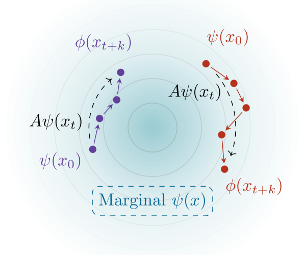
Figure 1: We apply temporal contrastive learning to observation pairs to obtain representations ($\psi(x_{0}),\psi(x_{t+k})$) such that $A\psi(x_{0})$ is close to $\psi(x_{t+k})$. Using these representations and the fact that the marginal representation distribution converges to a Gaussian, the distribution over intermediate representations has a closed form solution corresponding to linear interpolation between the initial and final representations.

Many prior works aim to learn representations such that are easy to predict while retaining salient bits of information. For time-series data, we want the representation to remain a sufficient statistic for distributions related to time – for example, they should retain bits required to predict future states (or representations thereof). While generative methods [100; 102; 56; 26] have this property, they tend to be computationally expensive (see, e.g., [72]) and can be challenging to scale to high-dimensional observations.

In this paper, we will study how contrastive methods (which are discriminative, rather than generative) can perform inference over times series. Ideally, we want representations of observations $x$ to be a sufficient statistic for temporal relationships (e.g., does $x^{\prime}$ occur after $x$?) but need not retain other information about $x$ (e.g. the location of static objects). This intuition motivates us to study how contrastive representation learning methods [65; 81; 17; 87; 95] might be used to solve prediction and planning problems on time series data. While prior works in computer vision [16; 65] and natural language processing (NLP) [59] often study the geometry of learned representations, our results show how geometric operations such as interpolation are related to inference. Our analysis will focus on a regularized version of the symmetrized infoNCE objective [71], generating positive examples by sampling pairs of observations from the same time series data. We will study how representations learned in this way can facilitate two inference questions: prediction and planning. As a stepping stone, we will build upon prior work [89] to show that regularized contrastive learning should produce representations whose marginal distribution is an isotropic Gaussian distribution.

The main contribution of this paper is to demonstrate how intermediate and future time steps in a time series can be inferred easily using contrastive representations. This inference problem captures a number of practical tasks: interpolation, in-filling, and even planning and control, where the intermediate steps represent states between a stand and goal. While ordinarily these problems require an iterative inference or optimization procedure, with contrastive representations this can be done simply by inverting a low-dimensional matrix. In one special case, inference will correspond to linear interpolation. Our first step is to prove that, under certain assumptions, the distribution over future representations has a Gaussian distribution, with a mean that is a linear function of the initial state representation (Lemma 1). This paves the main to our main result (Lemma 2): given an initial and final state, we show that the posterior distribution over an intermediate state representations also follows a Gaussian distribution. Said in other words, the representations follow a Gauss-Markov chain, wherein any joint or conditional distribution can be computed by inverting a low-dimensional matrix [57; 92] (See Fig. 1). In one special case, inference will correspond to linearly interpolating between the representations of an initial state and final state. Sec. 5 provides numerical experiments.

2 Related Work

Representations for time-series data.

In applications ranging from robotics to vision to NLP, users often want to learn representations of observations from time series data such that the spatial arrangement of representations reflects the temporal arrangement of the observations [65; 59; 70; 27]. Ideally, these representations should retain information required to predict future observations and infer likely paths between pairs of observations. Many approaches use an autoencoder, learning representations that retain the bits necessary to reconstruct the input observation, while also regularizing the representations to compressed or predictable [43; 68; 45; 12; 103; 20]. A prototypical method is the sequential VAE [100], which is computationally expensive to train because of the reconstruction loss, but is easy to use for inference. Our work shares the aims of prior prior methods that attempt to linearize the dynamics of nonlinear systems [80; 91; 7; 23; 64; 63], including videos [33; 40]. Our work aims to retain uncertainty estimates over predictions (like the sequential VAE) without requiring reconstruction. Avoiding reconstruction is appealing practically because it decreases the computational requirements and number of hyperparameters; and theoretically because it means that representations only need to retain bits about temporal relationships and not about the bits required to reconstruct the original observation.

Contrastive Learning.

Contrastive learning methods circumvent reconstruction by learning representations that merely classify if two events were sampled from the same joint distribution [35; 18; 71]. When applied to representing states along trajectories, contrastive representations learn to classify whether two points lie on the same trajectory or not [65; 78; 29; 70; 96]. Empirically, prior work in computer vision and NLP has observed that contrastive learning acquires representations where interpolation between representations corresponds to changing the images in semantically meaningful ways [94; 97; 67; 19; 50; 59].

Our analysis will be structurally similar to prior theoretical analysis on explaining why word embeddings can solve analogies [48; 5; 2]. Our work will make a Gaussianity assumption similar to Arora et al., [5] and our Markov assumption is similar to the random walks analyzed in Arora et al., [5]; Hashimoto et al., [36]. Our paper builds upon and extends these results to answer questions such as: “what is the distribution over future observations representations?” and “what is the distribution over state (representations) that would occur on the path between one observation and another?” While prior work is primarily aimed at explaining the good performance of contrastive word embeddings (see, e.g., [5]), we are primarily interested in showing how similar contrastive methods are an effective tool for inference over high-dimensional time series data. Our analysis will show how representations learned via temporal contrastive learning (i.e., without reconstruction) are sufficient statistics for inferring future outcomes and can be used for performing inference on a graphical model (a problem typically associated with generative methods).

Goal-oriented decision making.

Much work on time series representations is done in service of learning goal-reaching behavior, an old problem [61; 46] that has received renewed attention in recent years [15; 14; 21; 98; 53; 76; 39; 37]. Some of the excitement in goal-conditioned RL is a reflection of the recent success of self-supervised methods in computer vision [73] and NLP [66]. Our analysis will study a variant of contrastive representation learning proposed in prior work for goal-conditioned RL [29; 78]. These methods are widespread, appearing as learning objectives for learning value functions [27; 29; 101; 86; 1; 52; 51; 60; 49; 90], as auxiliary objectives [77; 83; 60; 82; 9; 4; 13], in objectives for model-based RL [80; 32; 3; 58], and in exploration methods [34; 25]. Our analysis will highlight connections between these prior methods, the classic successor representation [24; 8], and probabilistic inference.

Planning. Planning lies at the core of many RL and control methods, allowing methods to infer the sequence of states and actions that would occur if the agent navigated from one state to a goal state. While common methods such as PRM [44] and RRT [47] focus on building random graphs, there is a strong community focusing on planning methods based on probabilistic inference [6; 85; 93]. The key challenge is scaling to high-dimensional settings. While semi-parametric methods make progress on this problem this limitation through semi-parametric planning [30; 28; 99], it remains unclear how to scale any of these methods to high-dimensional settings when states do not lie on a low-dimensional manifold. Our analysis will show how contrastive representations may lift this limitation, with experiments validating this theory on 39-dimensional and 46-dimensional tasks.

3 Preliminaries

Our aim is to learn representations of time series data such that the spatial arrangement of representations corresponds to the temporal arrangement of the underlying data: if one example occurs shortly after another, then they should be mapped to similar representations. This problem setting arises in many areas, including video understanding and reinforcement learning. To define this problem formally, we will define a Markov process with states $x_{t}$ indexed by time $t$: $p(x_{1:T}\mid x_{0})=\prod_{t=0}^{T}p(x_{t+1}\mid x_{t})$. The dynamics $p(x_{t+1}\mid x_{t})$ tell us the immediate next state, and we can define the distribution over states $t$ steps in the future by marginalizing over the intermediate states, $p_{t}(x_{t}\mid x_{0})=\int p(x_{1:t}\mid x_{0})\mathrm{d}x_{1:t-1}$. A key quantity of interest will be the $\gamma$-discounted state occupancy measure, which corresponds to a time-averaged distribution over future states:

$$p_{t+}(x_{t+}=x)=(1-\gamma)\sum_{t=0}^{\infty}\gamma^{t}p_{t}(x_{t}=x).$$ (1)

Contrastive learning. Our analysis will focus on applying contrastive learning to a particular data distribution. Contrastive learning [35; 65; 75] acquires representations using “positive” pairs $(x,x^{+})$ and “negative” pairs $(x,x^{-})$. While contrastive learning typically learns just one representation, we will use two different representation for the two elements of the pair; that is, our analysis will use terms like $\phi(x)$, $\psi(x^{+})$ and $\psi(x^{-})$. We assume all representations lie in $\mathbbm{R}^{k}$.

The aim of contrastive learning is to learn representations such that positive pairs have similar representations ($\phi(x)\approx\psi(x^{+})$) while negative pairs have dissimilar representations ($\phi(x)\neq\psi(x^{-})$). Let $p(x,x)$ be the joint distribution over positive pairs (i.e., $(x,x^{+})\sim p(x,x)$). We will use the product of the marginal distributions to sample negative pairs ($(x,x^{-})\sim p(x)p(x)$). Our analysis is based on the infoNCE objective without resubstitution [81; 65]:

$$\min_{\phi(\cdot),\psi(\cdot)}\quad \mathbb{E}_{\begin{subarray}{c}(x,x^{+})\sim p(x)\\ x_{1:B-1}^{-}\sim p(x)\end{subarray}}\left[\log\tfrac{e^{f(\phi(x),\psi(x^{+}))}}{e^{\sum_{i=1}^{B-1}e^{f(\phi(x)^{T},\psi(x_{i}^{-}))}}}\right].$$ (2)

Precisely, we will use the symmetrized version of this loss [71], once where the denominator is the sum across rows of a logits matrix and once where it is a sum across the columns.

While contrastive learning is typically applied to an example $x$ and an augmentation $x^{+}\sim p(x\mid x)$ of that same example (e.g., a random crop), we will follow prior work [78; 65] in using the time series dynamics to generate the positive pairs, so $x^{+}$ will be an observation that occurs temporally after $x$. While our experiments will sample positive examples from the discounted state occupancy measure ($x^{+}\sim p_{t+}(x_{t+}\mid x)$) in line with prior work [29], our analysis will also apply to different distributions (e.g., always sampling a state $k$ steps ahead).

While prior work typically constrains the representations to have a constant norm (i.e., to lie on the unit hypersphere) [65], we will instead constrain the expected norm of the representations is bounded, a difference that will be important for our analysis:

$$\tfrac{1}{k}\mathbb{E}_{p(x)}\left[\|\psi(x)\|_{2}^{2}\right]\leq c.$$ (3)

Because the norm scales with the dimension of the representation, we have scaled down the left side by the representation dimension, $k$. In practice, we will impose this constraint by adding a regularization term $\lambda\mathbb{E}_{p(x)}\left[\|\psi(x)\|_{2}^{2}\right]$ to the infoNCE objective (Eq. 2) and dynamically tuning the weight $\lambda$ via dual gradient descent.

3.1 Key assumptions

This section outlines the two key assumptions behind our analysis, both of which have some theoretical justification. Our main assumption examines the distribution over representations acquired by contrastive learning:

Assumption 1.

Regularized, temporal contrastive learning acquires representations whose marginal distribution representations $p(\psi)\triangleq\int p(x)\mathbbm{1}(\psi(x)=\psi)\mathrm{d}x$ is an isotropic Gaussian distribution:

$$p(\psi)={\mathcal{N}}(\psi;\mu=0,\sigma=c\cdot I).$$ (4)

In Appendix A.1 we extend prior work [89] provide some theoretical intuition for why this assumption should hold: namely, that the isotropic Gaussian is the distribution that maximizes entropy subject to an expected L2 norm constraint (Eq. 3) [79; 41; 22]. Our analysis also assumes that the learned representations converge to the theoretical minimizer of the infoNCE objective:

Assumption 2.

Applying contrastive learning to the symmetrized infoNCE objective results in representations that that encode a probability ratio:

$$e^{-\frac{1}{2}\|\phi(x_{0})-\psi(x)\|_{2}^{2}}=\frac{p_{t+}(x_{t+}=x\mid x_{0})}{p(x)C}.$$ (5)

This assumption holds under ideal conditions [54; 69], but we nonetheless call this an “assumption” because it may not hold in practice due to sampling and function approximation error. This assumption means the learned representations are sufficient statistics for predicting the probability (ratio) of future states: these representations must retain all the information pertinent to reasoning about temporal relationships, but need not retain information about the precise contents of the observations. As such, they may be much more compressed than representations learned via reconstruction.

Combined, these assumptions will allow us to express the distribution over sequences of representations as a Gauss-Markov chain. The denominator in Assumption 2, $p(x)$, may have a complex distribution, but Assumption 1 tells us that the distribution over representations has a simpler form. This will allow us to rearrange Assumption 2 to express the conditional distribution over representations as the product of two Gaussian likelihoods. Note that the left hand side of Assumption 2 already looks like a Gaussian likelihood.

4 Contrastive Representations Make Inference Easy

In this section, we will show how representations learned by (regularized) contrastive learning are distributed according to a Gauss-Markov chain, making it straightforward to perform inference (e.g., planning, prediction) over these representations. Our proof technique will combine (known) results about Gaussian distributions with (known) results about contrastive learning to produce a result that is not known (to the best of our knowledge): representations learned by temporal contrastive learning are distributed according to a Gauss-Markov chain. We start by discussing an important choice of parametrization (Sec. 4.1) that facilitates prediction (Sec. 4.2) before presenting the main result in Sec. 4.3.

4.1 A Parametrization for Shared Encoders

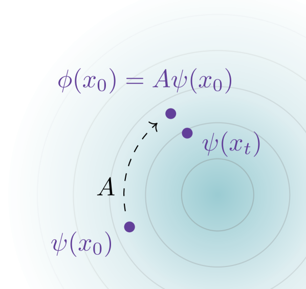
Figure 2: A parametrization for temporal contrastive learning.

This section describes the two encoders ($\psi(\cdot),\phi(\cdot)$) to compute representations of $x$ and $x^{+}$. While prior work in computer vision and NLP literature use the same encoder for both $x$ and $x^{+}$, this decision does not make sense for many time-series data as it would imply that our prediction for $p(x_{t}\mid x_{0})$ is the same as our prediction for $p(x_{0}\mid x_{t})$. However, the difficulty of transiting from $x_{0}$ to $x_{t}$ (e.g., climbing to the peak of a mountain) might be more difficult that the reverse (e.g., sledding down a mountain). We will propose a parametrization that will be important for using these representations for planning.

We will treat the encoder $\psi(\cdot)$ as encoding the contents of the state. We will additionally learn a matrix $A$ so that the function $\psi\mapsto A\psi$ corresponds to a (multi-step) prediction of the future representation. To map this onto contrastive learning, we will use $\phi(x)\triangleq A\psi(x)$ as the encoder for the initial state. One way of interpreting this encoder is as an additional linear projection applied on top of $\psi(\cdot)$, a design similar to those used in other areas of contrastive learning [18]. Once learned, we can use these encoders to answer questions about prediction (Sec. 4.2) and planning (Sec. 4.3).

4.2 Representations Encode a Predictive Model

Given an initial state $x_{0}$, what states are likely to occur in the future? Answering this question directly in terms of high-dimensional states is challenging, but our learned

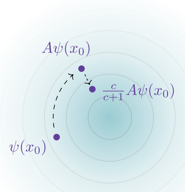
Figure 3: Predicting representations of future states.

representations provide a straightforward answer.

Let $\psi_{0}=\psi(x_{0})$ and $\psi_{t+}=\psi(x_{t+})$ be random variables representing the representations of the initial state and a future state. Our aim is to estimate the distribution over these future representations, $p(\psi_{t+}\mid\psi_{0})$. We will show that the learned representations encode this distribution.

Lemma 1.

Under the assumptions from Sec. 3, the distribution over representations of future states follows a Gaussian distribution with mean parameter given by the initial state representation:

$$p(\psi_{t+}=\psi\mid\psi_{0})={\mathcal{N}}\Bigl{(}\mu=\frac{c}{c+1}A\psi_{0},\Sigma=\frac{c}{c+1}I\Bigr{)}.$$ (6)

The main takeaway here is that the distribution over future representations has a convenient, closed form solution. The representation norm constraint, $c$, determines the shrinkage factor $\frac{c}{c+1}\in[0,1)$; highly regularized settings (small $c$) move the mean closer towards the origin and decrease the variance, as visualized in Fig. 3. Regardless of the constraint $c$, the predicted mean is a linear function $\psi\mapsto\frac{c}{c+1}A\psi$.

Proof.

Our proof technique will be similar to that of the law of the unconscious statistician:

$$\textstyle p( \textstyle\psi_{t+}\mid\psi_{0})\stackrel{{\scriptstyle(a)}}{{=}}\tfrac{p(\psi_{t+}\mid\psi_{0})}{\cancel{p(\psi_{0})}}$$

$$\textstyle\propto\iint p(\psi_{t+},x_{t+},\psi_{0},x_{0})\mathrm{d}x_{t+}\mathrm{d}x_{0}$$

$$\textstyle\stackrel{{\scriptstyle(b)}}{{=}}\iint p(\psi_{t+}\mid x_{t+})p(\psi_{0}\mid x_{0})p(x_{t+}\mid x_{0})p(x_{0})\mathrm{d}x_{t+}\mathrm{d}x_{0}$$

$$\textstyle\stackrel{{\scriptstyle(c)}}{{\propto}}\iint\mathbbm{1}(\psi(x_{t+})=\psi_{t+})\mathbbm{1}(\psi(x_{0})=\psi_{0})$$

$$\textstyle\qquad p(x_{t+})e^{-\frac{1}{2}\|A\psi(x_{0})-\psi(x)\|_{2}^{2}}p(x_{0})\mathrm{d}x_{t+}\mathrm{d}x_{0}$$

$$\textstyle\stackrel{{\scriptstyle(d)}}{{=}}e^{-\frac{1}{2}\|A\psi_{0}-\psi_{t+}\|_{2}^{2}}\iint\mathbbm{1}(\psi(x_{t+})=\psi_{t+})$$

$$\textstyle\qquad\mathbbm{1}(\psi(x_{0})=\psi_{0})p(x_{t+})p(x_{0})\mathrm{d}x_{t+}\mathrm{d}x$$

$$\textstyle\stackrel{{\scriptstyle(e)}}{{=}}e^{-\frac{1}{2}\|A\psi_{0}-\psi_{t+}\|_{2}^{2}}$$

$$\textstyle\qquad\underbrace{\left(\int p(x_{t+})\mathbbm{1}(\psi(x_{t+}))\mathrm{d}x_{t+}\right)}_{p(\psi_{t+})}\underbrace{\left(\int p(x_{0})\mathbbm{1}(\psi(x_{0})\mathrm{d}x_{0}\right)}_{p(\psi_{0})}$$

$$\textstyle\stackrel{{\scriptstyle(f)}}{{\propto}}e^{-\frac{1}{2}\|A\psi_{0}-\psi_{t+}\|_{2}^{2}}e^{-\frac{1}{2c}\|\psi_{t+}\|_{2}^{2}}e^{-\frac{1}{2c}\|\psi_{0}\|_{2}^{2}}$$

$$\textstyle\stackrel{{\scriptstyle(g)}}{{\propto}}e^{-\frac{1+\frac{1}{c}}{2}\|\frac{1}{1+\frac{1}{c}}A\psi_{0}-\psi_{t+}\|_{2}^{2}}$$

$$\textstyle\propto{\mathcal{N}}\left(\psi_{t+};\mu=\tfrac{c}{c+1}A\psi_{0},\Sigma=\tfrac{c}{c+1}I\right).$$

In (a) we applied Bayes’ Rule and removed the denominator, which is a constant w.r.t. $\psi_{t+}$. In (b) we factored the joint distribution, noting that $\psi_{t+}$ and $\psi_{0}$ are deterministic functions of $x_{t+}$ and $x_{0}$ respectively, so they are conditionally independent from the other random variables. In (c) we used Assumption 2 after solving for $p(x_{t+}\mid x_{0})=p(x_{t+})e^{-\frac{1}{2}\|A\psi(x_{0})-\psi(x)\|_{2}^{2}}$. In (d) we noted that when the integrand is nonzero, it takes on a constant value of $e^{-\frac{1}{2}\|A\psi_{0}-\psi_{t+}\|_{2}^{2}}$, so we can move that constant outside the integral. In (e) we used the definition of the marginal representation distribution (Eq. 6). In (f) we used Assumption 1 to write the marginal distributions $p(\psi_{t+})$ and $p(\psi_{0})$ as Gaussian distributions. We removed the normalizing constants, which are independent of $\psi_{t+}$. In (g) we completed the square and then recognized the expression as the density of a multivariate Gaussian distribution. ∎

4.3 Planning over One Intermediate State

We now show how these representations can be used for a specific type of planning: given an initial state $x_{0}$ and a future state $x_{t+}$, infer the representation of an intermediate “waypoint” state $x_{w}$. The next section will extend this analysis to inferring the entire sequence of intermediate states. We assume $x_{0}\rightarrow x_{w}\rightarrow x_{t+}$ form a Markov chain where $x_{w}\sim p(x_{t+}\mid x_{0}=x_{0})$ and $x_{t+}\sim p(x_{t+}\mid x_{0}=x_{w})$ are both drawn from the discounted state occupancy measure (Eq. 1). Let random variable $\psi_{w}=\psi(x_{w})$ be the representation of this intermediate state. Our main result is that the posterior distribution over waypoint representations has a closed form solution in terms of the initial state representation and future state representation:

Lemma 2.

Under Assumptions 1 and 2, the posterior distribution over waypoint representations is a Gaussian whose mean and covariance are linear functions of the initial and final state representations:

$$p(\psi_{w}\mid\psi_{0},\psi_{t+})=\mathcal{N}\Bigl{(}\psi_{w};\mu \,{\color[rgb]{0,0,0}=\Sigma^{-1}(A^{T}\psi_{t+}+A\psi_{0})},$$

$$\Sigma \,{\color[rgb]{0,0,0}=\tfrac{c}{c+1}A^{T}A+\tfrac{c+1}{c}I}\Bigr{)}.$$

The proof (Appendix A.2) uses the Markov property together with Lemma 1. The main takeaway from this lemma is that the posterior distribution takes the form of a simple probability distribution (a Gaussian) with parameters that are linear functions of the initial and final representations.

We give three examples to build intuition:

1. Example 1: $A=I$ and the $c$ is very large (little regularization). Then, the covariance is $\Sigma\approx 2I$ and the mean is the simple average of the initial and final representations $\mu\approx\frac{1}{2}(\psi_{0}+\psi_{t+})$. In other words, the waypoint representation is the midpoint of the line $\psi_{0}\rightarrow\psi_{t+}$.

2. Example 2: $A$ is a rotation matrix and $c$ is very large. Rotation matrices satisfy $A^{T}=A^{-1}$ so the covariance is again $\Sigma\approx 2I$. As noted in Sec. 4.2, we can interpret $A\psi_{0}$ as a prediction of which representations will occur after $\psi_{0}$. Similarly, $A^{-1}\psi_{t+}=A^{T}\psi_{t+}$ is a prediction of which representations will occur before $\psi_{t+}$. Lemma 2 tells us that the mean of the waypoint distribution is the simple average of these two predictions, $\mu\approx\frac{1}{2}(A^{T}\psi_{t+}+A\psi_{0})$.

3. Example 3: $A$ is a rotation matrix and $c=0.01$ (very strong regularization). In this case $\Sigma=\frac{0.01}{0.01+1}A^{T}A+\frac{0.01+1}{0.01}I\approx 100I$, so $\mu\approx\frac{1}{100}(\psi_{0}+\psi_{t+})\approx 0$. Thus, in the case of strong regularization, the posterior concentrates around the origin.

4.4 Planning over Many Intermediate States

This section extends the analysis to multiple intermediate states. Again, we will infer the posterior distribution of the representations of these intermediate states, $\psi_{w_{1}},\psi_{w_{2}},\cdots$. We assume that these states form a Markov chain.

Lemma 3.

Given observations from a Markov chain $x_{0}\rightarrow x_{1}\cdots x_{t+}$, the joint distribution over representations is a Gaussian distribution. Using $\psi_{1:n}=\begin{pmatrix}\psi_{w_{1}},\cdots,\psi_{w_{n}}\end{pmatrix}$ to denote the concatenated representations of each observation, we can write this distribution as

$$p(\psi_{1:n})\propto\exp\bigl{(}-\tfrac{1}{2}\psi_{1:n}^{T}\Sigma^{-1}\psi_{1:n}+\eta^{T}\psi_{1:n}\bigr{)},$$

where $\Sigma^{-1}$ is a tridiagonal matrix

$$\Sigma^{-1} =\left(\begin{smallmatrix}\frac{c}{c+1}A^{T}A+\frac{c+1}{c}I&-A^{T}&&\\ -A&\frac{c}{c+1}A^{T}A+\frac{c+1}{c}I&-A^{T}&\\[-8.61108pt] &&&\ddots\\ \end{smallmatrix}\right),$$

$$\text{and}\;\eta =\left(\begin{smallmatrix}A\psi_{0}\\ 0\\[-3.0pt] \vdots\\ A^{T}\psi_{t+}\end{smallmatrix}\right).$$

This distribution can be written in the canonical parametrization as $\Sigma=\Lambda^{-1}$ and $\mu=\Sigma\eta$. Recall that Gaussian distributions are closed under marginalization. Thus, once in this canonical parametrization, the marginal distributions can be obtained by reading off individual entries of these parameters:

$$p(\psi_{i}\mid\psi_{0},\psi_{t+})={\mathcal{N}}\left(\psi_{i};\mu_{i}=(\Sigma\eta)^{(i)},\Sigma_{i}=(\Lambda^{-1})^{(i,i)}\right).$$

The key takeaway here is that this posterior distribution over waypoints is Gaussian, and it has a closed form expression in terms of the initial and final representations (as well as regularization parameter $c$ and the learned matrix $A$).

In the general case of $n$ intermediate states, the posterior distribution is

$$p(\psi_{w_{1}}\cdots\psi_{w_{n}}\mid\psi_{0},\psi_{t+}) \propto e^{-\frac{1+\frac{1}{c}}{2}\sum_{i=1}^{n}\|\frac{c}{c+1}A\psi_{w_{i}}-\psi_{w_{i+1}}\|_{2}^{2}},$$

where $\psi_{w_{0}}=\psi_{0}$ and $\psi_{w_{n+1}}=\psi_{t+}$. This corresponds to a chain graphical model with edge potentials $f(\psi,\psi^{\prime})=e^{-\frac{1+\frac{1}{c}}{2}\|\frac{c}{c+1}A\psi-\psi^{\prime}\|_{2}^{2}}$.

Special case.

To build intuition, consider the special case where $A$ is a rotation matrix and $c$ is very large, so $\frac{c}{c+1}A^{T}A+\frac{c+1}{c}\approx 2I$. In this case, $\Sigma^{-1}$ is a (block) second difference matrix [38]:

$$\Sigma^{-1}=\left(\begin{smallmatrix}2I&-I&&\\ -I&2I&-I&\\[-4.30554pt] &&&\ddots\end{smallmatrix}\right).$$

The inverse of this matrix has a closed form solution [62, Pg. 471], allowing us to obtain the mean of each waypoint in closed form:

$$\mu_{i}=(1-\lambda(i))\psi_{0}+\lambda(i)A^{T}\psi_{t+},$$ (7)

where $\lambda(i)=\tfrac{i}{n+1}$. Thus, each posterior mean is a convex combination of the (forward prediction from the) initial representation and the (backwards prediction from the) final representation. When $A$ is the identity matrix, the posterior mean is simple linear interpolation between the initial and final representations!

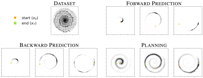
Figure 4: Numerical simulation of our analysis. (Top Left)  Toy dataset of time-series data consisting of many outwardly-spiraling trajectories. We apply temporal contrastive learning to these data. (Top Right)  For three initial observations ($\blacksquare$), we use the learned representations to predict the distribution over future observations. Note that these distributions correctly capture the spiral structure. (Bottom Left)  For three observations ($\star$), we use the learned representations to predict the distribution over preceding observations. (Bottom Right)  Given an initial and final observation, we plot the inferred posterior distribution over the waypoint (Sec. 4.3). The representations capture the shape of the distribution.

5 Numerical Simulation

We include several didactic experiments to illustrate our results. Code to reproduce these results, including all hyperparameters, is available at Synthetic Dataset To validate our analysis, we design a time series task with 2D points where inference over intermediate points (i.e., in-filling) requires nonlinear interpolation. Fig. 4 (Top Left) shows the dataset of time series data, starting at the origin and spiraling outwards, with each trajectory using a randomly-chosen initial angle. We applied contrastive learning with the parametrization in Sec. 4.1 to these data. We then used these representations to solve prediction and planning problems using the derivations in Sec. 4.2 and Sec. 4.3.

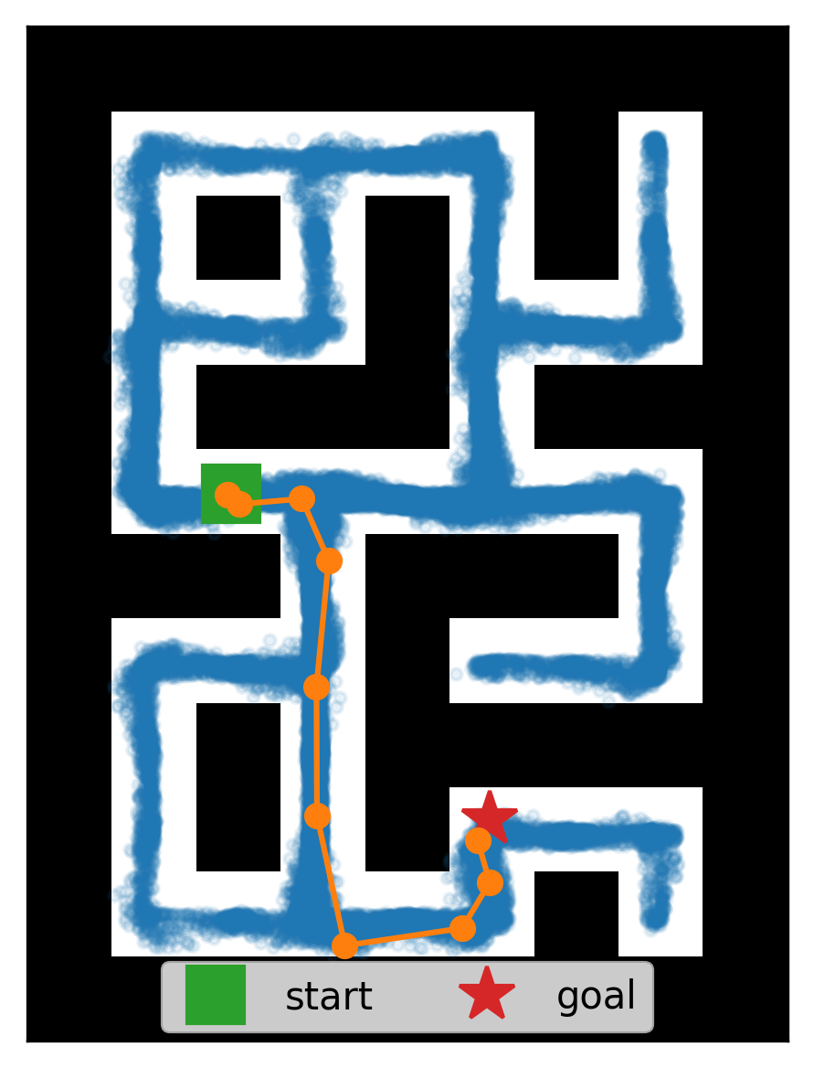
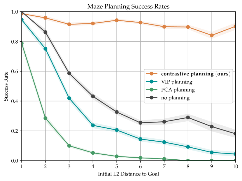
Figure 5: Using inferred paths over our contrastive representations for control boosts success rates by $4.5\times$ on the most difficult goals ($18\%\rightarrow 84\%$). Alternative representation learning techniques fail to improve performance when used for planning.

Fig. 4 (Top Right) shows forward predictions, while Fig. 4 (Bottom Left) shows backwards predictions. Note that these predictions correctly handle the nonlinear structure of these data – states nearby the initial state in Euclidean space that are not temporally adjacent are assigned low likelihood. Fig. 4 (Bottom Right) shows the posterior distribution over one waypoint.

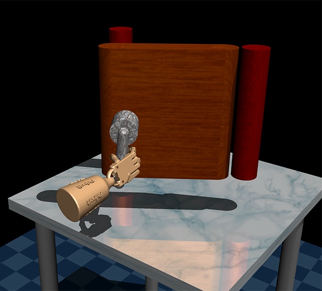
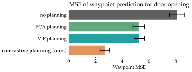
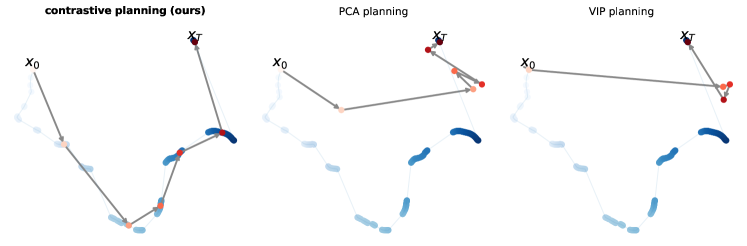
Figure 6: Planning for 39-dimensional robotic door opening. (Top Left)  We use a dataset of trajectories demonstrating door opening from prior work [31] to learn representations. (Top Right)  We use our method and three baselines to infer one intermediate waypoint between the first and last observation in a trajectory from a held-out validation set. Errors are measured using the mean squared error with the true waypoint observation; predicted representations are converted to observations using nearest neighbors on a validation set. (Bottom)  We visualize a TSNE of the states along the sampled trajectory as blue circles, with the transparency indicating the index along the trajectory. (Bottom)  We visualize the inferred plan (Sec. 4.3) as red circles connected by arrows, comparing with plans generated using representations from PCA and VIP. Our contrastive representations plan waypoints that better fit the intermediate states of trajectory.

5.1 Solving Mazes with Inferred Representations

Our next experiment studies whether the inferred representations are useful for solving a control task. We took a 2d maze environment and dataset from prior work (Fig. 5, Left) [31] and learned encoders from this dataset. To solve the maze, we take the observation of the starting state and goal state, compute the representations of these states, and use the analysis in Sec. 4.3 to infer the sequence of intermediate representations. We visualize the results using a nearest neighbor retrieval (Fig. 5, Left). Appendix Fig. 7 contains additional examples.

Finally, we studied whether these representations are useful for control. We implemented a simple proportional controller for this maze. As expected, this proportional controller can successfully navigate to close goals, but fails to reach distant goals (Fig. 5, Right). However, if we use the proportional controller to track a series of waypoints planned using our representations (i.e., the orange dots shown in Fig. 5 (Left)), the success rate increases by up to $4.5\times$. To test the importance of nonlinear representations, we compare with a “PCA” baseline that predicts waypoints by interpolating between the principal components of the initial state and goal state. The better performance of our method indicates the importance of doing the interpolation using representations that are nonlinear functions of the input observations. While prior methods learn representations to encode temporal distances, it is unclear whether these methods support inference via interpolation. To test this hypothesis, we use one of these methods (“VIP” [52]) as a baseline. While the VIP representations likely encode similar bits as our representations, the better performance of the contrastive representations indicates that the VIP representations do not expose those bits in a way that makes planning easy.

5.2 Higher dimensional tasks

In this section we provide preliminary experiments showing the planning approach in Sec. 4 scales to higher dimensional tasks. We used two datasets from prior work [31]: door-human-v0 (39-dimensional observations) and hammer-human-v0 (46-dimensional observations). After learning encoders on these tasks, we evaluated the inference capabilities of the learned representations. Given the first and last observation from a trajectory in a validation set, we use linear interpolation (see Eq. 7) to infer the representation of five intermediate waypoints representations.

We evaluate performance in two ways. Quantitatively, we measure the mean squared error between each of the true waypoint observations and those inferred by our method. Since our method infers representations, rather than observations, we use a nearest-neighbor retrieval on a validation set so that we can measure errors in the space of observations. Qualitatively, we visualize the high-dimensional observations from the validation trajectory using a 2-dimensional TSNE embedding, overlying the infer waypoints from our method; as before, we convert the representations inferred by our method to observations using nearest neighbors.

We compare with three alternative methods in Figures 6. To test the importance of representation learning, we first naïvely interpolate between the initial and final observations (“no planning”). The poor performance of this baseline indicates that the input time series are highly nonlinear. Similarly, interpolating the principle components of the initial and final observations (“PCA”) performs poorly, again highlighting that the input time series is highly nonlinear and that our representations are doing more than denoising (i.e., discarding directions of small variation). The third baseline, “VIP” [52], learns representations to encode temporal distances using approximate dynamic programming. Like our method, VIP avoids reconstruction and learns nonlinear representations of the observations. However, the results in Fig. 6 highlight that VIP’s representations do not allow users to plan by interpolation. The error bars shown in Fig. 6 (Top Right) show the standard deviation over 500 trajectories sampled from the validation set. For reproducibility, we repeated this entire experiment on another task, the 46-dimensional hammer-human-v0 from D4RL. The results, shown in Appendix Fig. 8, support the conclusions above. Taken together, these results show that our procedure for interpolating contrastive representations continues to be effective on tasks where observations have dozens of dimensions.

6 Discussion

Representation learning is at the core of many high-dimensional time-series modeling questions, yet how those representations are learned is often disconnected with the inferential task. The main contribution of this paper is to show how discriminative techniques can be used to acquire compact representations that make it easy to answer inferential questions about time. The precise objective and parametrization we studied is not much different from that used in practice, suggesting that either our theoretical results might be adapted to the existing methods, or that practitioners might adopt these details so they can use the closed-form solutions to inference questions. Our work may also have implications for studying the structure of learned representations. While prior work often studies the geometry of representations as a post-hoc check, our analysis may provide tools for studying when interpolation properties are guaranteed to emerge, as well as how to learn representations with certain desired geometric properties.

Limitations.

Our analysis hinges on the two assumptions mentioned in Sec. 3.1, and it remains open how errors in those approximations translate into errors in our analysis. One important open question is whether it is always possible to satisfy these assumptions using sufficiently-expressive representations. We look forward to applying the results of this paper to applications in science and engineering.

Acknowledgements.

We thank Seohong Park, Gautam Reddy, and anonymous reviewers for feedback and discussions that shaped this project. This work was supported by Princeton Research Computing resources at Princeton University. This work was partially supported by AFOSR FA9550-22-1-0273.

Appendix A Proofs

A.1 Marginal Distribution over Representations is Gaussian

The infoNCE objective (Eq. 2) can be decomposed into an alignment term and a uniformity term [89], where the uniformity term can be simplified as follows:

$$\mathbb{E}_{x\sim p(x)}\left[\log\mathbb{E}_{x^{-}\sim p(x)}\left[e^{-\frac{1}{2}\|A\psi(x^{-})-\psi(x)\|_{2}^{2}}\right]\right]$$

$$=\frac{1}{N}\sum_{i=1}^{N}\log\bigg{(}\frac{1}{N-1}\sum_{j=1\cdots N,j\neq i}e^{-\frac{1}{2}\|A\psi(x_{i})-\psi(x_{j})\|_{2}^{2}}\bigg{)}$$

$$=\frac{1}{N}\sum_{i=1}^{N}\log\bigg{(}\frac{1}{N-1}\sum_{j=1\cdots N,j\neq i}\underbrace{\frac{1}{(2\pi)^{k/2}}e^{-\frac{1}{2}\|A\psi(x_{i})-\psi(x_{j})\|_{2}^{2}}}_{{\mathcal{N}}(\mu=\psi(x_{j});\Sigma=I)}\bigg{)}+\frac{k}{2}\log(2\pi)$$

$$=\frac{1}{N}\sum_{i=1}^{N}\log\hat{p}_{\textsc{GMM}}(\psi(x_{i}))+\frac{k}{2}\log(2\pi)$$

$$=-\hat{{\mathcal{H}}}[\psi(x)]+\frac{k}{2}\log(2\pi).$$

The derivation above extends that in Wang and Isola, [89] by considering a Gaussian distribution rather than a von Mises Fisher distribution. We are implicitly making the assumption that the marginal distributions satisfy $p(x)=p(x^{-})$. This difference corresponds to our choice of using a negative squared L2 distance in the infoNCE loss rather than an inner product, a difference that will be important later in our analysis. A second difference is that we do not use the resubstitution estimator (i.e., we exclude data point $x_{i}$ from our estimate of $\hat{p}_{\text{GMM}}$ when evaluating the likelihood of $x_{i}$), which we found hurt performance empirically. The takeaway from this identity is that maximizing the uniformity term corresponds to maximizing (an estimate of) the entropy of the representations.

We next prove that the maximum entropy distribution with an expected L2 norm constraint is a Gaussian distribution. Variants of this result are well known [79; 41; 22], but we include a full proof here for transparency.

Lemma 4.

The maximum entropy distribution satisfying the expected L2 norm constraint in Eq. 3 is a multivariate Gaussian distribution with mean $\mu=0$ and covariance $\Sigma=c\cdot I$

Proof.

We start by defining the corresponding Lagrangian, with the second constraint saying that $p(x)$ must be a valid probability distribution.

$${\mathcal{L}}(p)={\mathcal{H}}_{p}[x]+\lambda_{1}\left(\mathbb{E}_{p(x)}\left[\|x\|_{2}^{2}\right]-c\cdot k\right)+\lambda_{2}\left(\int p(x)\mathrm{d}x-1\right)$$

We next take the derivative w.r.t. $p(x)$:

$$\frac{\partial{\mathcal{L}}}{\partial p(x)}=-p(x)/p(x)-\log p(x)+\lambda_{1}\|x\|_{2}^{2}+\lambda_{2}$$

Setting this derivative equal to 0 and solving for $p(x)$, we get

$$p(x)=e^{-1+\lambda_{2}+\lambda_{1}\|x\|_{2}^{2}}.$$

We next solve for $\lambda_{1}$ and $\lambda_{2}$ to satisfy the constraints in the Lagrangian. Note that $x\sim{\mathcal{N}}(\mu=0,\Sigma=c\cdot I)$ has an expected norm $\mathbb{E}[\|x\|_{2}^{2}]=c\cdot k$, so we must have $\lambda_{1}=-\frac{1}{2c}$. We determine $\lambda_{1}$ as the normalizing constant for a Gaussian, finally giving us:

$$p(x)=\frac{1}{(2c\pi)^{k/2}}e^{\frac{-1}{2c}\|x\|_{2}^{2}}$$

corresponding to an isotropic Gaussian distribution with mean $\mu=0$ and covariance $\Sigma=c\cdot I$. ∎

A.2 Proof of Lemma 2: Waypoint Distribution

Proof.

$$p(\psi_{w}\mid\psi_{0},\psi_{t+}) \stackrel{{\scriptstyle(a)}}{{=}}\frac{p(\psi_{t+}\mid\psi_{w})p(\psi_{w}\mid\psi_{0})}{\cancel{p(\psi_{t+}\mid\psi_{0})}}$$

$$\stackrel{{\scriptstyle(b)}}{{\propto}}e^{-\frac{1+\frac{1}{c}}{2}\|\frac{c}{c+1}A\psi_{w}-\psi_{t+}\|_{2}^{2}}e^{-\frac{1+\frac{1}{c}}{2}\|\frac{c}{c+1}A\psi_{0}-\psi_{w}\|_{2}^{2}}$$

$$\stackrel{{\scriptstyle(c)}}{{\propto}}e^{-\frac{1}{2}(\psi_{w}-\mu)^{T}\Sigma(\psi_{w}-\mu)}\quad\text{where}\;\Sigma=\frac{c}{c+1}A^{T}A+\frac{c+1}{c}I,\;\mu=\Sigma^{-1}(A^{T}\psi_{t+}+A\psi_{0}).$$

$$={\mathcal{N}}(\psi_{w};\mu,\Sigma).$$

∎

In line (a) we used the definition of the conditional distribution and then simplified the numerator using the Markov property. Line (b) uses the Lemma 1. Line (c) completes the square, using $\stackrel{{\scriptstyle\text{const.}}}{{=}}$ to denote equality up to an additive constant that is independent of $\psi_{w}$, and using the definitions of $\mu$ and $\Sigma$ above:

$$\frac{c+1}{c}\left(\left\|\frac{c}{c+1}A\psi_{w}-\psi_{t+}\right\|_{2}^{2}+\left\|\frac{c}{c+1}A\psi_{0}-\psi_{w}\right\|_{2}^{2}\right)$$

$$=\frac{c+1}{c}\left(\psi_{w}^{T}(\frac{c}{c+1}A)^{T}(\frac{c}{c+1}A)\psi_{w}-2\psi_{t+}^{T}(\frac{c}{c+1}A)\psi_{w}+\cancel{\psi_{t+}^{T}\psi_{t+}}\right.$$

$$\qquad\left.+\cancel{\psi_{0}^{T}(\frac{c}{c+1}A)^{T}(\frac{c}{c+1}A)\psi_{0}}-2\psi_{0}^{T}(\frac{c}{c+1}A)^{T}\psi_{w}+\psi_{w}^{T}\psi_{w}\right)$$

$$\stackrel{{\scriptstyle\text{const.}}}{{=}}\psi_{w}^{T}(\underbrace{\frac{c}{c+1}A^{T}A+\frac{c+1}{c}I}_{\Sigma})\psi_{w}-2(A^{T}\psi_{t+}+A\psi_{0})^{T}\psi_{w}$$

$$\stackrel{{\scriptstyle\text{const.}}}{{=}}(\psi_{w}-\mu)^{T}\Sigma(\psi_{w}-\mu),$$

where $\Sigma=\frac{c}{c+1}A^{T}A+\frac{c+1}{c}I$ and $\mu=\Sigma^{-1}(A^{T}\psi_{t+}+A\psi_{0})$.

A.3 Proof of Lemma 3: Planning over Many Intermediate States

Proof.

We start by recalling that the waypoints form a Markov chain, so we can express their joint density as a product of conditional densities:

$$p(\psi_{1:n})=p(\psi_{0})p(\psi_{1}\mid\psi_{0})p(\psi_{2}\mid\psi_{1})\cdots p(\psi_{n}\mid\psi_{n-1}).$$

The aim of this lemma is to express the joint distribution over multiple waypoints, given an initial and final state representation:

$$p(\psi_{1:n}\mid\psi_{0},\psi_{t+}) \stackrel{{\scriptstyle(a)}}{{=}}\frac{p(\psi_{1:n}\mid\psi_{0})p(\psi_{t+}\mid\psi_{n})}{\cancel{p(\psi_{t+}\mid\psi_{0})}}$$

$$\stackrel{{\scriptstyle(b)}}{{\propto}}p(\psi_{1}\mid\psi_{0})p(\psi_{2}\mid\psi_{1})\cdots p(\psi_{t+}\mid\psi_{n})$$

$$\stackrel{{\scriptstyle(c)}}{{\propto}}\exp\left(-\tfrac{1}{2}\tfrac{c+1}{c}\|\tfrac{c}{c+1}A\psi_{0}-\psi_{1}\|_{2}^{2}-\tfrac{1}{2}\tfrac{c+1}{c}\|\tfrac{c}{c+1}A\psi_{1}-\psi_{2}\|_{2}^{2}-\cdots-\tfrac{1}{2}\tfrac{c+1}{c}\|\tfrac{c}{c+1}A\psi_{n}-\psi_{t+}\|_{2}^{2}\right)$$

$$\stackrel{{\scriptstyle(d)}}{{=}}\exp\bigg{(}-\cancel{\tfrac{1}{2}\tfrac{c}{c+1}\psi_{0}^{T}A^{T}A\psi_{0}}+\psi_{0}^{T}A^{T}\psi_{1}-\tfrac{1}{2}\tfrac{c+1}{c}\psi_{1}^{T}\psi_{1}$$

$$\qquad\qquad-\tfrac{1}{2}\tfrac{c}{c+1}\psi_{1}^{T}A^{T}A\psi_{1}+\psi_{1}^{T}A^{T}\psi_{2}-\tfrac{1}{2}\tfrac{c+1}{c}\psi_{2}^{T}\psi_{2}$$

$$\qquad\qquad-\tfrac{1}{2}\tfrac{c}{c+1}\psi_{2}^{T}A^{T}A\psi_{2}+\psi_{2}^{T}A^{T}\psi_{3}-\tfrac{1}{2}\tfrac{c+1}{c}\psi_{3}^{T}\psi_{3}$$

$$\kern 113.81102pt\vdots$$

$$\qquad\qquad-\tfrac{1}{2}\tfrac{c}{c+1}\psi_{n}^{T}A^{T}A\psi_{n}+\psi_{n}^{T}A^{T}\psi_{t+}-\cancel{\tfrac{1}{2}\tfrac{c+1}{c}\psi_{t+}^{T}\psi_{t+}}\bigg{)}$$

$$=\exp\bigl{(}-\tfrac{1}{2}\psi_{1:n}^{T}\Sigma^{-1}\psi_{1:n}+\eta^{T}\psi_{1:n}\bigr{)},$$

where $\Sigma^{-1}$ is a tridiagonal matrix

$$\Sigma^{-1} =\begin{pmatrix}\frac{c}{c+1}A^{T}A+\frac{c+1}{c}I&-A^{T}&&\\ -A&\frac{c}{c+1}A^{T}A+\frac{c+1}{c}I&-A^{T}&\\ &-A&\frac{c}{c+1}A^{T}A+\frac{c+1}{c}I&\\[-2.00749pt] &&&\ddots\hskip 3.01125pt\\[5.01874pt] \end{pmatrix}\quad\text{and}\;\eta=\begin{pmatrix}A\psi_{0}\\ 0\\[-3.44444pt] \vdots\\[-6.88889pt] \\ 0\\ A^{T}\psi_{t+}\end{pmatrix}.$$

In (a) we applied Bayes’ rule and removed the denominator because it is a constant with respect to $\psi_{1:n}$. In (b) we applied the Markov assumption. In (c) we used Lemma 1 to express the conditional probabilities as Gaussians, ignoring the proportionality constants (which are independent of $\psi$. In (d) we simplified the exponents, removing terms that do not depend on $\psi_{1:n}$ ∎

Appendix B Additional Experiments

Fig. 7 visualizes the inferred waypoints from the task in Fig. 5.

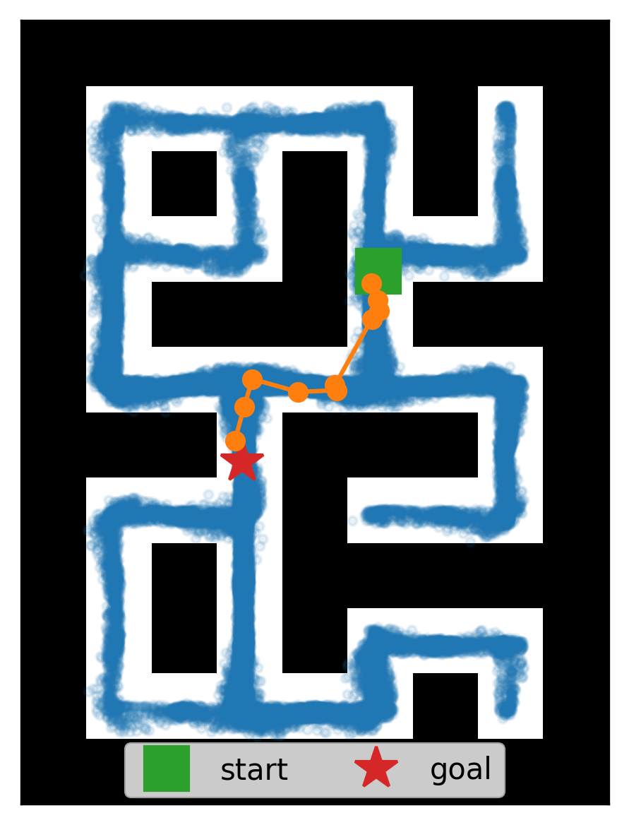
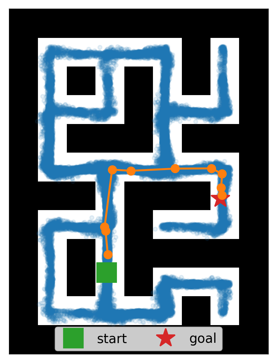
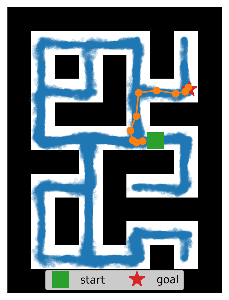
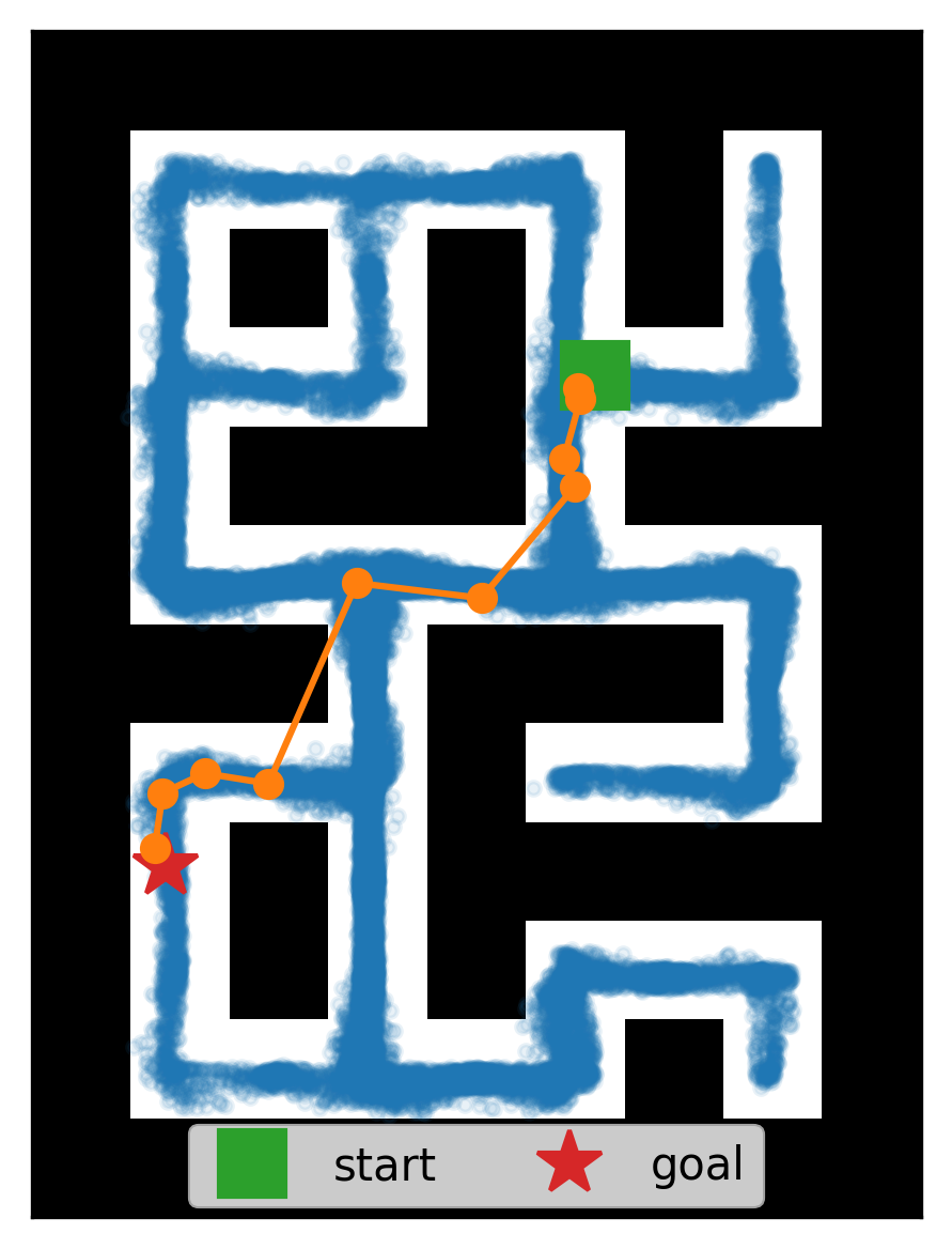
Figure 7: Our approach enables a goal-conditioned policy to reach farther targets (red) from the start (green) by planning over intermediate waypoints (orange).

Fig. 8 visualizes the representations learned on a 46-dimensional robotic hammering task (see Sec. 5.2).

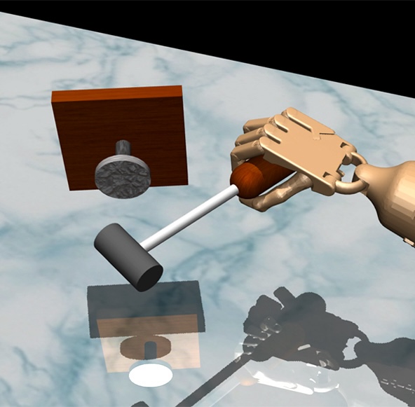
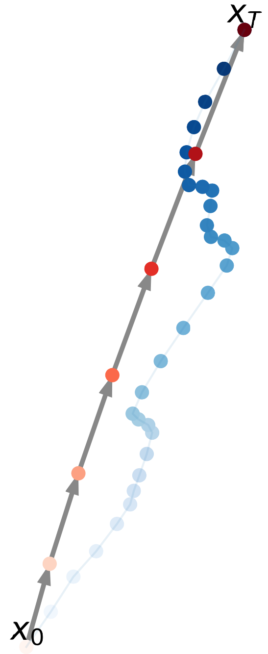
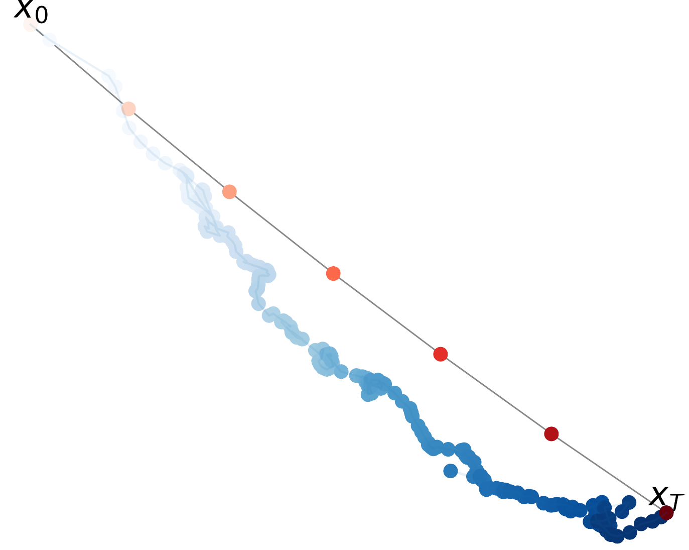
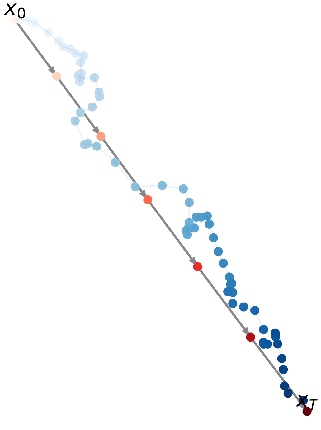
(a) Contrastive representations

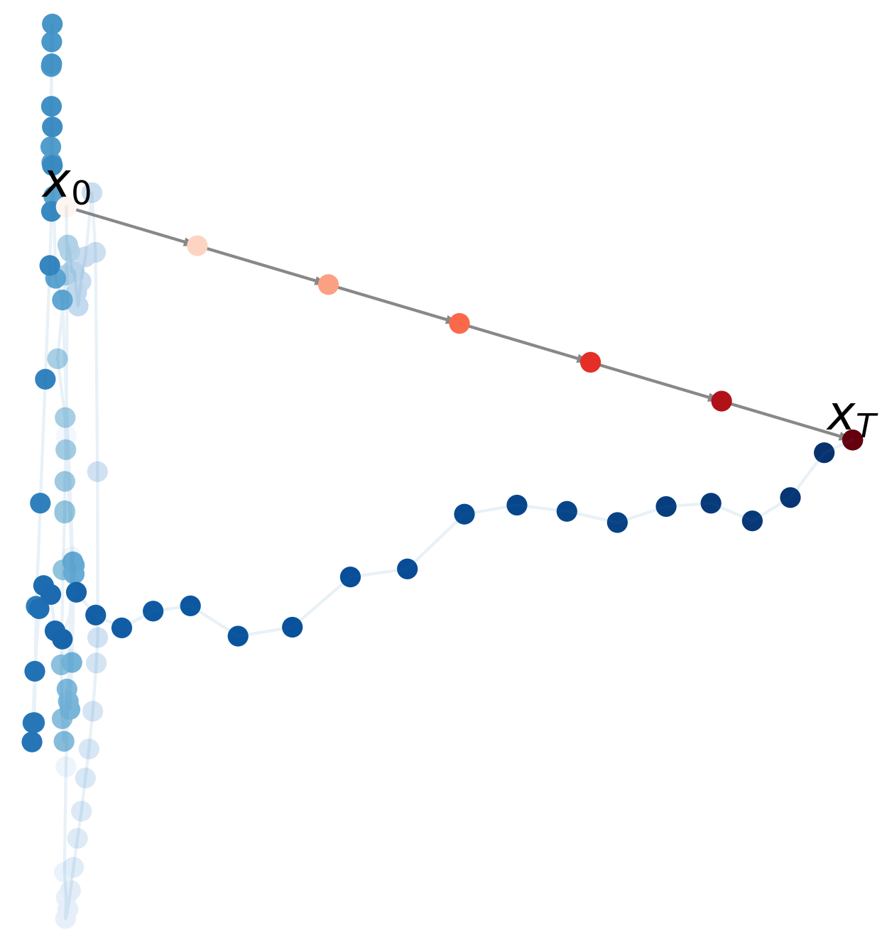
(b) PCA representations

Figure 8: Planning for 46-dimensional robotic hammering. (Left)  A dataset of trajectories demonstrating a hammer knocking a nail into a board [31]. (Center)  We visualize the learned representations as blue circles, with the transparency indicating the index of that observation along the trajectory. We also visualize the inferred plan (Sec. 4.3) as red circles connected by arrows. (Right)  Representations learned by PCA on the same trajectory as (a, left).

References

- Agarwal et al., [2019] Agarwal, A., Jiang, N., Kakade, S. M., and Sun, W. (2019). Reinforcement learning: Theory and algorithms. CS Dept., UW Seattle, Seattle, WA, USA, Tech. Rep, pages 10–4.
- Allen and Hospedales, [2019] Allen, C. and Hospedales, T. (2019). Analogies explained: Towards understanding word embeddings. In International Conference on Machine Learning, pages 223–231. PMLR.
- Allen, [2021] Allen, C. S. (2021). Learning markov state abstractions for deep reinforcement learning. In Neural Information Processing Systems.
- Anand et al., [2019] Anand, A., Racah, E., Ozair, S., Bengio, Y., Côté, M.-A., and Hjelm, R. D. (2019). Unsupervised state representation learning in atari. Advances in neural information processing systems, 32.
- Arora et al., [2016] Arora, S., Li, Y., Liang, Y., Ma, T., and Risteski, A. (2016). A latent variable model approach to pmi-based word embeddings. Transactions of the Association for Computational Linguistics, 4:385–399.
- Attias, [2003] Attias, H. (2003). Planning by Probabilistic Inference. In International Workshop on Artificial Intelligence and Statistics, pages 9–16. PMLR.
- Banijamali et al., [2018] Banijamali, E., Shu, R., Bui, H., Ghodsi, A., et al. (2018). Robust locally-linear controllable embedding. In International Conference on Artificial Intelligence and Statistics, pages 1751–1759. PMLR.
- Barreto et al., [2017] Barreto, A., Dabney, W., Munos, R., Hunt, J. J., Schaul, T., van Hasselt, H. P., and Silver, D. (2017). Successor features for transfer in reinforcement learning. Advances in neural information processing systems, 30.
- Bharadhwaj et al., [2021] Bharadhwaj, H., Babaeizadeh, M., Erhan, D., and Levine, S. (2021). Information prioritization through empowerment in visual model-based rl. In International Conference on Learning Representations.
- Botvinick and Toussaint, [2012] Botvinick, M. and Toussaint, M. (2012). Planning as inference. Trends in cognitive sciences, 16(10):485–488.
- Box et al., [2015] Box, G. E., Jenkins, G. M., Reinsel, G. C., and Ljung, G. M. (2015). Time series analysis: forecasting and control. John Wiley & Sons.
- Carroll et al., [2022] Carroll, M., Paradise, O., Lin, J., Georgescu, R., Sun, M., Bignell, D., Milani, S., Hofmann, K., Hausknecht, M., Dragan, A., et al. (2022). UniMASK: Unified Inference in Sequential Decision Problems.
- Castro et al., [2021] Castro, P. S., Kastner, T., Panangaden, P., and Rowland, M. (2021). Mico: Improved representations via sampling-based state similarity for markov decision processes. In Neural Information Processing Systems.
- Chane-Sane et al., [2021] Chane-Sane, E., Schmid, C., and Laptev, I. (2021). Goal-conditioned reinforcement learning with imagined subgoals. In International Conference on Machine Learning, pages 1430–1440. PMLR.
- Chen et al., [2021] Chen, L., Lu, K., Rajeswaran, A., Lee, K., Grover, A., Laskin, M., Abbeel, P., Srinivas, A., and Mordatch, I. (2021). Decision transformer: Reinforcement learning via sequence modeling. Advances in neural information processing systems, 34:15084–15097.
- [16] Chen, T., Kornblith, S., Norouzi, M., and Hinton, G. (2020a). A simple framework for contrastive learning of visual representations. In International conference on machine learning, pages 1597–1607. PMLR.
- [17] Chen, X., Fan, H., Girshick, R., and He, K. (2020b). Improved baselines with momentum contrastive learning. arXiv preprint arXiv:2003.04297.
- Chen and He, [2021] Chen, X. and He, K. (2021). Exploring simple siamese representation learning. In Proceedings of the IEEE/CVF conference on computer vision and pattern recognition, pages 15750–15758.
- Chen et al., [2019] Chen, Y.-C., Xu, X., Tian, Z., and Jia, J. (2019). Homomorphic Latent Space Interpolation for Unpaired Image-To-Image Translation. In 2019 IEEE/CVF Conference on Computer Vision and Pattern Recognition (CVPR), pages 2403–2411, Long Beach, CA, USA. IEEE.
- Chung et al., [2015] Chung, J., Kastner, K., Dinh, L., Goel, K., Courville, A. C., and Bengio, Y. (2015). A Recurrent Latent Variable Model for Sequential Data. In Advances in Neural Information Processing Systems, volume 28. Curran Associates, Inc.
- Colas et al., [2021] Colas, C., Karch, T., Sigaud, O., and Oudeyer, P.-Y. (2021). Intrinsically motivated goal-conditioned reinforcement learning: a short survey.
- Conrad, [2010] Conrad, K. (2010). Probability distributions and maximum likelihood.
- Cui et al., [2020] Cui, B., Chow, Y., and Ghavamzadeh, M. (2020). Control-aware representations for model-based reinforcement learning. In International Conference on Learning Representations.
- Dayan, [1993] Dayan, P. (1993). Improving generalization for temporal difference learning: The successor representation. Neural Computation, 5:613–624.
- Du et al., [2021] Du, Y., Gan, C., and Isola, P. (2021). Curious representation learning for embodied intelligence. 2021 IEEE/CVF International Conference on Computer Vision (ICCV), pages 10388–10397.
- Dumoulin et al., [2016] Dumoulin, V., Belghazi, I., Poole, B., Lamb, A., Arjovsky, M., Mastropietro, O., and Courville, A. (2016). Adversarially learned inference. In International Conference on Learning Representations.
- Eysenbach et al., [2020] Eysenbach, B., Salakhutdinov, R., and Levine, S. (2020). C-learning: Learning to achieve goals via recursive classification. In International Conference on Learning Representations.
- Eysenbach et al., [2019] Eysenbach, B., Salakhutdinov, R. R., and Levine, S. (2019). Search on the Replay Buffer: Bridging Planning and Reinforcement Learning. In Advances in Neural Information Processing Systems, volume 32. Curran Associates, Inc.
- Eysenbach et al., [2022] Eysenbach, B., Zhang, T., Levine, S., and Salakhutdinov, R. R. (2022). Contrastive learning as goal-conditioned reinforcement learning. Advances in Neural Information Processing Systems, 35:35603–35620.
- Fang et al., [2023] Fang, K., Yin, P., Nair, A., Walke, H. R., Yan, G., and Levine, S. (2023). Generalization with lossy affordances: Leveraging broad offline data for learning visuomotor tasks. In Conference on Robot Learning, pages 106–117. PMLR.
- Fu et al., [2020] Fu, J., Kumar, A., Nachum, O., Tucker, G., and Levine, S. (2020). D4rl: Datasets for deep data-driven reinforcement learning. arXiv preprint arXiv:2004.07219.
- Ghugare et al., [2022] Ghugare, R., Bharadhwaj, H., Eysenbach, B., Levine, S., and Salakhutdinov, R. (2022). Simplifying model-based rl: Learning representations, latent-space models, and policies with one objective. In The Eleventh International Conference on Learning Representations.
- Goroshin et al., [2015] Goroshin, R., Mathieu, M. F., and LeCun, Y. (2015). Learning to linearize under uncertainty. Advances in neural information processing systems, 28.
- Guo et al., [2022] Guo, Z., Thakoor, S., Pîslar, M., Avila Pires, B., Altché, F., Tallec, C., Saade, A., Calandriello, D., Grill, J.-B., Tang, Y., et al. (2022). Byol-explore: Exploration by bootstrapped prediction. Advances in neural information processing systems, 35:31855–31870.
- Gutmann and Hyvärinen, [2010] Gutmann, M. and Hyvärinen, A. (2010). Noise-contrastive estimation: A new estimation principle for unnormalized statistical models. In Proceedings of the Thirteenth International Conference on Artificial Intelligence and Statistics, pages 297–304. JMLR Workshop and Conference Proceedings.
- Hashimoto et al., [2016] Hashimoto, T. B., Alvarez-Melis, D., and Jaakkola, T. S. (2016). Word embeddings as metric recovery in semantic spaces. Transactions of the Association for Computational Linguistics, 4:273–286.
- Hejna et al., [2023] Hejna, J., Gao, J., and Sadigh, D. (2023). Distance weighted supervised learning for offline interaction data. arXiv preprint arXiv:2304.13774.
- Higham, [2022] Higham, N. (2022). What is the second difference matrix? https://nhigham.com/2022/01/31/what-is-the-second-difference-matrix/.
- Janner et al., [2021] Janner, M., Li, Q., and Levine, S. (2021). Offline reinforcement learning as one big sequence modeling problem. Advances in neural information processing systems, 34:1273–1286.
- Jayaraman and Grauman, [2016] Jayaraman, D. and Grauman, K. (2016). Slow and steady feature analysis: higher order temporal coherence in video. In Proceedings of the IEEE Conference on Computer Vision and Pattern Recognition, pages 3852–3861.
- Jaynes, [1957] Jaynes, E. T. (1957). Information Theory and Statistical Mechanics. Physical Review, 106(4):620–630.
- Jónsson et al., [1998] Jónsson, H., Mills, G., and Jacobsen, K. W. (1998). Nudged elastic band method for finding minimum energy paths of transitions. In Classical and quantum dynamics in condensed phase simulations, pages 385–404. World Scientific.
- Karamcheti et al., [2023] Karamcheti, S., Nair, S., Chen, A. S., Kollar, T., Finn, C., Sadigh, D., and Liang, P. (2023). Language-Driven Representation Learning for Robotics.
- Kavraki et al., [1996] Kavraki, L. E., Svestka, P., Latombe, J.-C., and Overmars, M. H. (1996). Probabilistic roadmaps for path planning in high-dimensional configuration spaces. IEEE transactions on Robotics and Automation, 12(4):566–580.
- Kenton and Toutanova, [2019] Kenton, J. D. M.-W. C. and Toutanova, L. K. (2019). Bert: Pre-training of deep bidirectional transformers for language understanding. In Proceedings of NAACL-HLT, pages 4171–4186.
- Laird et al., [1987] Laird, J. E., Newell, A., and Rosenbloom, P. S. (1987). Soar: An architecture for general intelligence. Artificial intelligence, 33(1):1–64.
- LaValle et al., [2001] LaValle, S. M., Kuffner, J. J., Donald, B., et al. (2001). Rapidly-exploring random trees: Progress and prospects. Algorithmic and computational robotics: new directions, 5:293–308.
- Levy and Goldberg, [2014] Levy, O. and Goldberg, Y. (2014). Linguistic regularities in sparse and explicit word representations. In Proceedings of the eighteenth conference on computational natural language learning, pages 171–180.
- Liu et al., [2023] Liu, B., Feng, Y., Liu, Q., and Stone, P. (2023). Metric residual network for sample efficient goal-conditioned reinforcement learning. In Proceedings of the AAAI Conference on Artificial Intelligence, volume 37, pages 8799–8806.
- Liu et al., [2018] Liu, X., Zou, Y., Kong, L., Diao, Z., Yan, J., Wang, J., Li, S., Jia, P., and You, J. (2018). Data Augmentation via Latent Space Interpolation for Image Classification. In 2018 24th International Conference on Pattern Recognition (ICPR), pages 728–733.
- Ma et al., [2023] Ma, Y. J., Kumar, V., Zhang, A., Bastani, O., and Jayaraman, D. (2023). LIV: Language-Image Representations and Rewards for Robotic Control.
- [52] Ma, Y. J., Sodhani, S., Jayaraman, D., Bastani, O., Kumar, V., and Zhang, A. (2022a). Vip: Towards universal visual reward and representation via value-implicit pre-training. In The Eleventh International Conference on Learning Representations.
- [53] Ma, Y. J., Yan, J., Jayaraman, D., and Bastani, O. (2022b). How far i’ll go: Offline goal-conditioned reinforcement learning via -advantage regression. arXiv preprint arXiv:2206.03023.
- Ma and Collins, [2018] Ma, Z. and Collins, M. (2018). Noise contrastive estimation and negative sampling for conditional models: Consistency and statistical efficiency. In Conference on Empirical Methods in Natural Language Processing.
- Majewski et al., [2017] Majewski, S. R., Schiavon, R. P., Frinchaboy, P. M., Prieto, C. A., Barkhouser, R., Bizyaev, D., Blank, B., Brunner, S., Burton, A., Carrera, R., et al. (2017). The apache point observatory galactic evolution experiment (apogee). The Astronomical Journal, 154(3):94.
- Makhzani et al., [2015] Makhzani, A., Shlens, J., Jaitly, N., Goodfellow, I., and Frey, B. (2015). Adversarial autoencoders. arXiv preprint arXiv:1511.05644.
- Malioutov et al., [2006] Malioutov, D. M., Johnson, J. K., and Willsky, A. S. (2006). Walk-sums and belief propagation in gaussian graphical models. The Journal of Machine Learning Research, 7:2031–2064.
- Mazoure et al., [2023] Mazoure, B., Eysenbach, B., Nachum, O., and Tompson, J. (2023). Contrastive value learning: Implicit models for simple offline rl. In Conference on Robot Learning, pages 1257–1267. PMLR.
- Mikolov et al., [2013] Mikolov, T., Chen, K., Corrado, G., and Dean, J. (2013). Efficient estimation of word representations in vector space. arXiv preprint arXiv:1301.3781.
- Nair et al., [2023] Nair, S., Rajeswaran, A., Kumar, V., Finn, C., and Gupta, A. (2023). R3m: A universal visual representation for robot manipulation. In Conference on Robot Learning, pages 892–909. PMLR.
- Newell et al., [1959] Newell, A., Shaw, J. C., and Simon, H. A. (1959). Report on a general problem solving program. In IFIP congress, volume 256, page 64. Pittsburgh, PA.
- Newman and Todd, [1958] Newman, M. and Todd, J. (1958). The evaluation of matrix inversion programs. Journal of the Society for Industrial and Applied Mathematics, 6(4):466–476.
- Nguyen et al., [2020] Nguyen, T., Shu, R., Pham, T., Bui, H., and Ermon, S. (2020). Non-markovian predictive coding for planning in latent space.
- Nguyen et al., [2021] Nguyen, T. D., Shu, R., Pham, T., Bui, H., and Ermon, S. (2021). Temporal predictive coding for model-based planning in latent space. In International Conference on Machine Learning, pages 8130–8139. PMLR.
- Oord et al., [2018] Oord, A. v. d., Li, Y., and Vinyals, O. (2018). Representation learning with contrastive predictive coding. arXiv preprint arXiv:1807.03748.
- OpenAI, [2023] OpenAI (2023). Gpt-4 technical report. ArXiv, abs/2303.08774.
- Oring et al., [2021] Oring, A., Yakhini, Z., and Hel-Or, Y. (2021). Autoencoder image interpolation by shaping the latent space. In International Conference on Machine Learning, pages 8281–8290. PMLR.
- Park and Lee, [2021] Park, S. and Lee, J. (2021). Finetuning Pretrained Transformers into Variational Autoencoders.
- Poole et al., [2019] Poole, B., Ozair, S., Van Den Oord, A., Alemi, A., and Tucker, G. (2019). On variational bounds of mutual information. In International Conference on Machine Learning, pages 5171–5180. PMLR.
- Qian et al., [2021] Qian, R., Meng, T., Gong, B., Yang, M.-H., Wang, H., Belongie, S., and Cui, Y. (2021). Spatiotemporal Contrastive Video Representation Learning. In Proceedings of the IEEE/CVF Conference on Computer Vision and Pattern Recognition, pages 6964–6974.
- Radford et al., [2021] Radford, A., Kim, J. W., Hallacy, C., Ramesh, A., Goh, G., Agarwal, S., Sastry, G., Askell, A., Mishkin, P., Clark, J., et al. (2021). Learning transferable visual models from natural language supervision. In International conference on machine learning, pages 8748–8763. PMLR.
- Razavi et al., [2019] Razavi, A., Van den Oord, A., and Vinyals, O. (2019). Generating diverse high-fidelity images with vq-vae-2. Advances in neural information processing systems, 32.
- Rombach et al., [2022] Rombach, R., Blattmann, A., Lorenz, D., Esser, P., and Ommer, B. (2022). High-resolution image synthesis with latent diffusion models. In Proceedings of the IEEE/CVF Conference on Computer Vision and Pattern Recognition, pages 10684–10695.
- Saelens et al., [2019] Saelens, W., Cannoodt, R., Todorov, H., and Saeys, Y. (2019). A comparison of single-cell trajectory inference methods. Nature biotechnology, 37(5):547–554.
- Saunshi et al., [2019] Saunshi, N., Plevrakis, O., Arora, S., Khodak, M., and Khandeparkar, H. (2019). A theoretical analysis of contrastive unsupervised representation learning. In International Conference on Machine Learning, pages 5628–5637. PMLR.
- Schroecker and Isbell, [2020] Schroecker, Y. and Isbell, C. (2020). Universal value density estimation for imitation learning and goal-conditioned reinforcement learning. arXiv preprint arXiv:2002.06473.
- Schwarzer et al., [2020] Schwarzer, M., Anand, A., Goel, R., Hjelm, R. D., Courville, A., and Bachman, P. (2020). Data-efficient reinforcement learning with self-predictive representations. In International Conference on Learning Representations.
- Sermanet et al., [2018] Sermanet, P., Lynch, C., Chebotar, Y., Hsu, J., Jang, E., Schaal, S., Levine, S., and Brain, G. (2018). Time-contrastive networks: Self-supervised learning from video. In 2018 IEEE international conference on robotics and automation (ICRA), pages 1134–1141. IEEE.
- Shannon, [1948] Shannon, C. E. (1948). A mathematical theory of communication. The Bell system technical journal, 27(3):379–423.
- Shu et al., [2020] Shu, R., Nguyen, T., Chow, Y., Pham, T., Than, K., Ghavamzadeh, M., Ermon, S., and Bui, H. (2020). Predictive coding for locally-linear control. In International Conference on Machine Learning, pages 8862–8871. PMLR.
- Sohn, [2016] Sohn, K. (2016). Improved deep metric learning with multi-class n-pair loss objective. Advances in neural information processing systems, 29.
- Stooke et al., [2021] Stooke, A., Lee, K., Abbeel, P., and Laskin, M. (2021). Decoupling representation learning from reinforcement learning. In International Conference on Machine Learning, pages 9870–9879. PMLR.
- Tang et al., [2023] Tang, Y., Guo, Z. D., Richemond, P. H., Pires, B. A., Chandak, Y., Munos, R., Rowland, M., Azar, M. G., Le Lan, C., Lyle, C., et al. (2023). Understanding self-predictive learning for reinforcement learning. In International Conference on Machine Learning, pages 33632–33656. PMLR.
- Theodorou et al., [2010] Theodorou, E., Buchli, J., and Schaal, S. (2010). A generalized path integral control approach to reinforcement learning. The Journal of Machine Learning Research, 11:3137–3181.
- Thijssen and Kappen, [2015] Thijssen, S. and Kappen, H. J. (2015). Path integral control and state-dependent feedback. Physical Review E, 91(3):032104.
- [86] Tian, S., Nair, S., Ebert, F., Dasari, S., Eysenbach, B., Finn, C., and Levine, S. (2020a). Model-based visual planning with self-supervised functional distances. In International Conference on Learning Representations.
- [87] Tian, Y., Krishnan, D., and Isola, P. (2020b). Contrastive multiview coding. In Computer Vision–ECCV 2020: 16th European Conference, Glasgow, UK, August 23–28, 2020, Proceedings, Part XI 16, pages 776–794. Springer.
- Uhlenbeck and Ornstein, [1930] Uhlenbeck, G. E. and Ornstein, L. S. (1930). On the theory of the brownian motion. Physical review, 36(5):823.
- Wang and Isola, [2020] Wang, T. and Isola, P. (2020). Understanding contrastive representation learning through alignment and uniformity on the hypersphere. In International Conference on Machine Learning, pages 9929–9939. PMLR.
- Wang et al., [2023] Wang, T., Torralba, A., Isola, P., and Zhang, A. (2023). Optimal goal-reaching reinforcement learning via quasimetric learning. In International Conference on Machine Learning. PMLR.
- Watter et al., [2015] Watter, M., Springenberg, J., Boedecker, J., and Riedmiller, M. (2015). Embed to control: A locally linear latent dynamics model for control from raw images. Advances in neural information processing systems, 28.
- Weiss and Freeman, [1999] Weiss, Y. and Freeman, W. (1999). Correctness of belief propagation in gaussian graphical models of arbitrary topology. Advances in neural information processing systems, 12.
- Williams et al., [2015] Williams, G., Aldrich, A., and Theodorou, E. (2015). Model Predictive Path Integral Control using Covariance Variable Importance Sampling.
- Wiskott and Sejnowski, [2002] Wiskott, L. and Sejnowski, T. J. (2002). Slow Feature Analysis: Unsupervised Learning of Invariances. Neural Computation, 14(4):715–770.
- Wu et al., [2018] Wu, Z., Xiong, Y., Yu, S. X., and Lin, D. (2018). Unsupervised feature learning via non-parametric instance discrimination. In Proceedings of the IEEE conference on computer vision and pattern recognition, pages 3733–3742.
- Xu et al., [2023] Xu, M., Xu, Z., Chi, C., Veloso, M., and Song, S. (2023). Xskill: Cross embodiment skill discovery. In Conference on Robot Learning, pages 3536–3555. PMLR.
- Yan et al., [2021] Yan, J.-W., Lin, C.-S., Yang, F.-E., Li, Y.-J., and Frank Wang, Y.-C. (2021). Semantics-Guided Representation Learning with Applications to Visual Synthesis. In 2020 25th International Conference on Pattern Recognition (ICPR), pages 7181–7187.
- Yang et al., [2021] Yang, R., Lu, Y., Li, W., Sun, H., Fang, M., Du, Y., Li, X., Han, L., and Zhang, C. (2021). Rethinking goal-conditioned supervised learning and its connection to offline rl. In International Conference on Learning Representations.
- Zhang et al., [2021] Zhang, T., Eysenbach, B., Salakhutdinov, R., Levine, S., and Gonzalez, J. E. (2021). C-planning: An automatic curriculum for learning goal-reaching tasks. In International Conference on Learning Representations.
- Zhao et al., [2017] Zhao, S., Song, J., and Ermon, S. (2017). Towards deeper understanding of variational autoencoding models. arXiv preprint arXiv:1702.08658.
- Zheng et al., [2024] Zheng, C., Eysenbach, B., Walke, H. R., Yin, P., Fang, K., Salakhutdinov, R., and Levine, S. (2024). Stabilizing contrastive RL: Techniques for robotic goal reaching from offline data. In The Twelfth International Conference on Learning Representations.
- [102] Zhu, Y., Min, M. R., Kadav, A., and Graf, H. P. (2020a). S3vae: Self-supervised sequential vae for representation disentanglement and data generation. In Proceedings of the IEEE/CVF Conference on Computer Vision and Pattern Recognition, pages 6538–6547.
- [103] Zhu, Y., Min, M. R., Kadav, A., and Graf, H. P. (2020b). S3VAE: Self-Supervised Sequential VAE for Representation Disentanglement and Data Generation.