Directional Smoothness and Gradient Methods: Convergence and Adaptivity

Abstract

We develop new sub-optimality bounds for gradient descent (GD) that depend on the conditioning of the objective along the path of optimization, rather than on global, worst-case constants. Key to our proofs is directional smoothness, a measure of gradient variation that we use to develop upper-bounds on the objective. Minimizing these upper-bounds requires solving implicit equations to obtain a sequence of strongly adapted step-sizes; we show that these equations are straightforward to solve for convex quadratics and lead to new guarantees for two classical step-sizes. For general functions, we prove that the Polyak step-size and normalized GD obtain fast, path-dependent rates despite using no knowledge of the directional smoothness. Experiments on logistic regression show our convergence guarantees are tighter than the classical theory based on $L$-smoothness.

1 Introduction

Gradient methods for differentiable functions are typically analyzed under the assumption that $f$ is $L$-smooth, meaning $\nabla f$ is $L$-Lipschitz continuous. This condition implies $f$ is upper-bounded by a quadratic and guarantees that gradient descent (GD) with step-size $\eta<2/L$ decreases the optimality gap at each iteration (Bertsekas, 1997). However, experience shows that GD can still decrease the objective when $f$ is not $L$-smooth, particularly for deep neural networks (Bengio, 2012; Li et al., 2020; Cohen et al., 2021). Even for functions verifying smoothness, convergence rates are often pessimistic and fail to predict optimization speed in practice (Paquette et al., 2023).

One way to avoid global smoothness of $f$ is to use local Lipschitz continuity of the gradient (“local smoothness”). Local smoothness uses different Lipschitz constants for different neighbourhoods, thus avoiding global assumptions and obtaining improved rates. However, such analyses typically require the iterates to be bounded, in which case local smoothness reduces to $\tilde{L}$-smoothness over a compact set (Malitsky & Mishchenko, 2020). Boundedness can be enforced in a variety of ways: Zhang & Hong (2020) break optimization into stages, Patel & Berahas (2022) develop a stopping-time framework, and Lu & Mei (2023) use line-search and a modified update. These approaches either modify the underlying optimization algorithm, require local smoothness oracles (Park et al., 2021), or rely on highly complex arguments.

In contrast, we prove simple sub-optimality bounds for gradient descent without global smoothness assumptions by deriving upper-bounds of the form,

$$f(x_{k+1}) \leq f(x_{k})+\left\langle\nabla f(x_{k}),x_{k+1}-x_{k}\right\rangle$$ (1)

$$\hskip 20.00003pt+\frac{M(x_{k+1},x_{k})}{2}\|x_{k+1}-x_{k}\|_{2}^{2},$$

where the directional smoothness function $M(x_{k+1},x_{k})$ depends only on properties of $f$ along the chord between $x_{k+1}$ and $x_{k}$. Our bounds provide a path-dependent perspective on GD and are tighter than conventional analyses when the step-size sequence is adapted to the directional smoothness, meaning $\eta_{k}<2/M(x_{k+1},x_{k})$. See Figure 1 for two real-data examples highlighting our improvement over classical rates. We summarize all our contributions as follows.

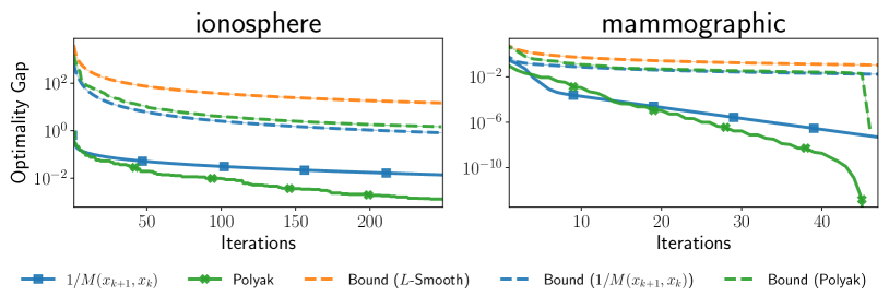
Figure 1: Comparison of actual (solid lines) and theoretical (dashed lines) convergence rates for GD with step-sizes adapted to the directional smoothness ($\eta_{k}=1/M(x_{k+1},x_{k})$) and GD with the Polyak step-size. Both problems are non-strongly convex logistic regressions on datasets from the UCI repository (Asuncion & Newman, 2007). Our new bounds using directional smoothness are tighter than those based on global $L$-smoothness of $f$ and adapt to the optimization path. For example, on mammographic our theoretical rate for the Polyak step-size concentrates rapidly exactly when the optimizer shows fast convergence.

Directional Smoothness. We introduce two related directional smoothness functions $M(y,x)$; one depends only on the end-points $y,x$ and is easily computed, while the other yields a tighter bound but depends on the chord $\mathcal{C}=\left\{\alpha x+(1-\alpha)y:\alpha\in[0,1]\right\}$. We show that the first notion of directional smoothness is a valid notion of smoothness for any differentiable and convex function, without assuming that global smoothness holds at all. We show the second notion is valid for all differentiable functions.

Sub-optimality bounds. We leverage these directional smoothness functions to prove new sub-optimality bounds for GD on convex functions as well as functions satisfying a new directional strong convexity assumption. Our bounds (given in Section 3) are localized to the GD trajectory, hold for any possible step-size sequence, and are tighter than the classic analysis based on $L$-smoothness. They are also more general than the classical analysis since we do not need to assume that $f$ is globally $L$–smooth in order to show progress; all we require is a sequence of step-sizes adapted to the directional smoothness function.

Adaptive Step-Sizes in the Quadratic Case. In the general setting, computing step-sizes which are adapted to the directional smoothness requires solving a challenging non-linear root-finding problem. For quadratic problems, we show that the ideal step-size that satisfies $\eta_{k}=1/M(x_{k+1},x_{k})$ is the Rayleigh quotient and is connected to the hedging algorithm (Altschuler & Parrilo, 2023).

Exponential Search. Moving beyond quadratics, we prove that the equation $\eta_{k}=1/M(x_{k+1},x_{k})$ admits at least one solution under mild conditions, meaning ideal step-sizes can be computed using Newton’s method. Since computing these step-sizes is typically impractical, we instead adapt exponential search (Carmon & Hinder, 2022) to obtain similar path-dependent complexities up to a log-log penalty.

Polyak and Normalized GD. More importantly, we show that the Polyak step-size (Polyak, 1987) and normalized GD achieve fast, path-dependent rates without knowledge of the directional smoothness. Our analysis reveals that the Polyak step-size adapts to any directional smoothness to obtain the tightest possible convergence rate. This property is not shared by constant step-size GD and may explain the superiority of the Polyak step-size in many settings.

1.1 Additional Related Work

Directional smoothness can be viewed as a relaxation of non-uniform smoothness (Mei et al., 2021), which restricts the smoothness function $M$ to depend only on the origin point, $x$. Mei et al. (2021) develop methods which leverage non-uniform smoothness and a non-uniform version of the Łojasiewicz inequality to break classical lower-bounds for first-order optimization. Similar work by Berahas et al. (2023) shows that a weaker local smoothness oracle is also sufficient to break lower bounds for gradient methods. A major advantage of our work over these oracle-based approaches is that we construct explicit directional smoothness functions which can be evaluated in hindsight.

Our work is closely connected to that by Malitsky & Mishchenko (2020), who use a smoothed $M(y,x)$ to set the step-size. Vladarean et al. (2021) apply a similar step-size to primal-dual hybrid gradient methods, while Zhao & Huang (2024) relate directional smoothness to Barzilai-Borwein updates (Barzilai & Borwein, 1988) and Vainsencher et al. (2015) use local smoothness in neighbourhoods of the global minimizer to set the step-size for SVRG. Finally, Orabona (2023) show convergence bounds that depend on the smoothness in the direction of the optimal set, whereas we are interested in smoothness over the optimization trajectory.

Finally, we note that adaptivity to directional smoothness is different from adaptivity to the sequence of observed gradients obtained by methods such as Adagrad  (Duchi et al., 2010; Streeter & McMahan, 2010). Adagrad and its variants are most useful when the gradients are bounded, such as in Lipschitz optimization, although they can also be used to obtain rates for smooth functions (Levy, 2017). We do not address adaptivity to gradients in this work.

2 Directional Smoothness

We say that the function $f$ is $L$-smooth if for all $x,y\in\mathbb{R}^{d}$,

$$f(y)\leq f(x)+\left\langle\nabla f(x),y-x\right\rangle+\frac{L}{2}\|y-x\|_{2}^{2}.$$ (2)

Minimizing this quadratic upper bound in $y$ gives the classical GD update with step-size $\eta_{k}=1/L$. However, this viewpoint gives rates which depend on the global, worst-case growth of $f$. This is both counter-intuitive and undesirable because the iterates of GD,

$$x_{k+1}=x_{k}-\eta_{k}\nabla f(x_{k}),$$ (3)

depend only on local properties of $f$. Intuitively, the analysis should also depend only on the local conditioning along the optimization path $\left\{x_{1},x_{2},\ldots\right\}$. Towards this end, we generalize the smoothness upper-bound as follows:

Definition 2.1.

We call $M:\mathbb{R}^{d}\times\mathbb{R}^{d}\rightarrow\mathbb{R}_{+}$ a directional smoothness function for $f$ if for all $x,y\in\mathbb{R}^{d}$,

$$f(y)\leq f(x)\!+\!\left\langle\nabla f(x),y\!-\!x\right\rangle\frac{M(y,x)}{2}{\left\lVert y\!-\!x\right\rVert}^{2}.$$ (4)

If a function is $L$-smooth, then $M(x,y)=L$ is a trivial choice of directional smoothness function. In the rest of this section, we construct different $M$ functions that provide tighter bounds on $f$ while still being possible to evaluate. The first is the point-wise directional smoothness,

$$D(y,x):=\frac{2\|\nabla f(y)-\nabla f(x)\|_{2}}{\|y-x\|_{2}}.$$ (5)

Point-wise smoothness is a directional estimate of $L$ and satisfies $D(y,x)\leq 2L$. Indeed, $L$ can be equivalently defined as the supremum of $D(x,y)/2$ over the domain of $f$ (Beck, 2017). When $f$ is convex and differentiable, $D(x,y)$ satisfies Definition 2.1.

Lemma 2.2.

If $f$ is convex and differentiable, then the point-wise directional smoothness (Equation 5) satisfies,

$$f(y)\leq f(x)+\left\langle\nabla f(x),y-x\right\rangle+\frac{D(y,x)}{2}\|y-x\|_{2}^{2}.$$ (6)

See Appendix A (we defer all proofs to the relevant appendices). However, in the worst-case, the point-wise directional smoothness $D$ is weaker than the standard upper-bound $M(x,y)=L$ by a factor of two. This factor of two is not an artifact of the analysis and is generally unavoidable, as the next proposition shows.

Proposition 2.3.

There exists a convex, differentiable $f$ s.t.

$$\begin{split}f(y)\leq f(x)&+\left\langle\nabla f(x),y-x\right\rangle\\ &\qquad+\frac{t\|\nabla f(x)-\nabla f(y)\|}{2\|y-x\|_{2}}\|y-x\|^{2}_{2}\end{split}$$ (7)

does not hold for all $x,y\in\mathbb{R}^{d}$ if $t<2$.

While the point-wise smoothness is easy to compute, this additional factor of two can make Equation 6 looser than $L$-smoothness — on isotropic quadratics, for example. As an alternative, we define the path-wise directional smoothness,

$$A(x,y):=\sup_{t\in[0,1]}\frac{\left\langle\nabla f(x\!+\!t(y\!-\!x))\!-\!\nabla f(x),y\!-\!x\right\rangle}{t\|y\!-\!x\|^{2}},$$ (8)

and show that it verifies the quadratic upper-bound and satisfies Definition 2.1 even without convexity.

Lemma 2.4.

For any differentiable function $f$, the path-wise smoothness (8) satisfies

$$f(y)\leq f(x)+\left\langle\nabla f(x),y-x\right\rangle+\frac{A(y,x)}{2}\|y-x\|_{2}^{2}.$$ (9)

Path smoothness is tighter than point-wise directional smoothness since $A(y,x)\leq D(y,x)$, but hard to compute because it depends on the chord between $x$ and $y$. That is, it depends on the properties of $f$ on the line $\left\{tx+(1-t)y:t\in[0,1]\right\}$ rather than solely on the points $x$ and $y$ like the point-wise smoothness.

Point-wise and path-wise smoothness are constructive, but they may not yield the tightest bounds in all situations. The tightest directional smoothness function, which we call the optimal point-wise smoothness, is defined to be the smallest number for which the quadratic upper bound holds,

$$H(y,x) =\frac{\left|f(y)-f(x)-\left\langle\nabla f(x),y-x\right\rangle\right|}{\frac{1}{2}{\left\lVert y-x\right\rVert}^{2}}$$ (10)

By definition, $H$ is the tightest possible directional smoothness function we can hope for; it lower bounds any constant $C$ that satisfies the quadratic bound Equation 2. Thus, $H(y,x)\leq M(y,x)$ for any $M(y,x)$.

The different notions of directional smoothness introduced in this section, including the optimal point-wise smoothness, represent different trade-offs between computability and tightness. Computing $H(x,y)$ requires access to both the function and gradient values, whereas the point-wise directional-smoothness $D(x,y)$ requires only access to the gradients and that $f$ be convex. On the other hand, the bound we established on the path-wise directional smoothness $A(x,y)$ in Lemma 2.4 holds with or without convexity, at the cost of a harder-to-compute function.

3 Path-Dependent Sub-Optimality Bounds

Figure 2: Illustration of GD with $\eta_{k}=1/L$. Even though the step-size exactly minimizes the upper-bound from $L$-smoothness, $M_{i}$ directional smoothness better predicts the progress of the gradient step. Our rates improve on $L$-smoothness because of this tighter bound.

Given directional smoothness $M$, we obtain a version of the descent lemma which depends only on local geometry,

$$f_{k+1}\leq f_{k}-\left(\eta_{k}-\frac{\eta_{k}^{2}M(x_{k+1},x_{k})}{2}\right)\|\nabla f(x_{k})\|_{2}^{2},$$ (11)

where $f_{k}=f(x_{k})$ and $f_{k+1}=f(x_{k+1})$ (see Lemma A.1). If $\eta_{k}<2/M(x_{k+1},x_{k})$, then GD is guaranteed to decrease the function value and we call $\eta_{k}$ adapted to $M(x_{k+1},x_{k})$. However, finding a sequence of adapted step-sizes is not always straightforward. For instance, computing $\eta_{k}=1/M(x_{k+1}(\eta_{k}),x_{k})$ requires solving a non-linear equation.

The rest of this section leverages directional smoothness to derive new guarantees for GD with arbitrary step-sizes. We emphasize that the following results are sub-optimality bounds, rather than convergence rates; a sequence of adapted step-sizes is required to convert our propositions into a convergence theory. As a trade-off, we obtain bounds reflecting the locality of GD, rather than treating it as a global method.

We start with the case when $f$ has lower curvature. Instead of using strong convexity or the PL-condition (Karimi et al., 2016), we propose the directional strong convexity constant,

$$\mu(y,x)\!=\!\inf_{t\in[0,1]}\frac{\left\langle\nabla f(x\!+\!t(y\!-\!x))\!-\!\nabla f(x),y\!-\!x\right\rangle}{t\|y-x\|_{2}^{2}}.$$ (12)

If $f$ is convex, then $\mu(y,x)$ is non-negative and verifies the standard lower-bound from strong convexity,

$$f(y)\geq f(x)+\left\langle\nabla f(x),y-x\right\rangle+\frac{\mu(y,x)}{2}\|y-x\|_{2}^{2}.$$ (13)

Moreover, we have $\mu(y,x)\geq\mu$ when $f$ is $\mu$–strongly convex. We prove two bounds for convex functions using directional strong convexity. For brevity, we denote $M_{i}:=M(x_{i+1},x_{i})$, $\mu_{i}:=\mu_{i}(x_{i+1},x_{i})$, $\delta_{i}=f(x_{i})-f(x^{*})$, and $\Delta_{i}=\|x_{i}-x^{*}\|_{2}^{2}$, where $x^{*}$ is a minimizer of $f$.

Proposition 3.1.

If $f$ is convex with minimizer $x^{*}$, then GD with step-size sequence $\left\{\eta_{k}\right\}$ satisfies,

$$\begin{split}\delta_{k}&\leq\left[\prod_{i\in\mathcal{G}}\left(1+\eta_{i}\lambda_{i}\mu_{i}\right)\right]\delta_{0}\\ &+\sum_{i\in\mathcal{B}}\left[\prod_{j>i,j\in\mathcal{G}}\left(1+\eta_{j}\lambda_{j}\mu_{j}\right)\right]\frac{\eta_{i}\lambda_{i}}{2}\|\nabla f(x_{i})\|_{2}^{2},\end{split}$$ (14)

where $\lambda_{i}\!=\!\eta_{i}M_{i}\!-\!2$, $\mathcal{G}=\left\{i:\eta_{i}\!<\!\frac{2}{M(x_{i+1},x_{i})}\right\}$, $\mathcal{B}=[k]\!\setminus\!\mathcal{G}$.

The analysis splits iterations into good steps $\mathcal{G}$, where $\eta_{k}$ is adapted to the directional smoothness, and bad steps $\mathcal{B}$, where the step-size is too large and GD may increase the optimality gap. When $f$ is $L$-smooth and $\mu$-strongly convex, using the step-size sequence $\eta_{k}=1/L$ gives

$$\frac{f(x_{k+1})-f(x^{*})}{f(x_{0})-f(x^{*})}\leq\left[\prod_{i=0}^{k}\left(1-\frac{\mu_{i}\left(2-M_{i}/L\right)}{L}\right)\right]$$ (15)

where $\mu_{i}\left(2-M_{i}/L\right)\geq\mu$. As a result, Equation 14 gives a at least as tight a rate under standard assumptions by localizing to the convergence path as described by any directional smoothness $M$. When $M_{k}<L$, the gap in constants yields a strictly improved rate, as shown by Figure 2. We also prove the following, more elegant bound.

Proposition 3.2.

If $f$ is convex with minimizer $x^{*}$, then GD with step-size sequence $\left\{\eta_{k}\right\}$ satisfies,

$$\begin{split}&\Delta_{k}\leq\left[\prod_{i=0}^{k}\left(1-\mu_{i}\eta_{i}\right)\right]\Delta_{0}\\ &\hskip 10.00002pt+\!\sum_{i=0}^{k}\left[\prod_{j>i}\left(1\!-\!\mu_{j}\eta_{j}\right)\right]\!\!\left(M_{i}\eta_{i}^{3}\!-\!\eta_{i}^{2}\right)\|\nabla f(x_{i})\|_{2}^{2}.\end{split}$$ (16)

Unlike Proposition 3.1, this analysis shows linear progress at each iteration and does not divide $k$ into good steps and bad steps. In exchange, the second term in Equation 16 reflects how much convergence is degraded when $\eta_{k}$ is not adapted to the directional smoothness function $M$.

We conclude this section with a bound for when there is no lower curvature, meaning $\mu_{i}=0$.

Proposition 3.3.

Let $\overline{x}_{k}=\sum_{i=0}^{k}\eta_{i}x_{i+1}/\sum_{i=0}^{k}\eta_{i}$. If $f$ is convex with minimizer $x^{*}$, then GD satisfies,

$$\begin{split}f(\overline{x}_{k})-f(x^{*})&\leq\frac{\|x_{0}-x^{*}\|_{2}^{2}}{2\sum_{i=0}^{k}\eta_{i}}\\ &+\frac{\sum_{i=0}^{k}\eta_{i}^{2}(\eta_{i}M_{i}-1)\|\nabla f(x_{i})\|_{2}^{2}}{2\sum_{i=0}^{k}\eta_{i}}.\end{split}$$ (17)

This rate is at least as tight as the standard analysis because $M_{i}\leq L.$ It is key to our developments in the next sections.

4 Adaptive Learning Rates

The main challenge in converting our sub-optimality bounds into convergence rates is the requirement for adapted step-sizes, meaning $\eta_{k}<2/M(x_{k+1},x_{k})$. Given an adapted step-size, the directional descent lemma (Equation 11) implies GD decreases the loss at step $k$ and we can obtain fast rates. However, $x_{k+1}$ is itself a function of $\eta_{k}$, meaning adapted step-sizes are not straightforward to compute.

If $f$ is $L$-smooth, then $M(x_{k+1},x_{k})\leq 2L$ for all the directional smoothness functions introduced so-far, meaning $\eta_{k}<\frac{1}{L}$ is trivially adapted. However, these step-sizes don’t capture any local properties of $f$, so we instead consider strongly adapted step-sizes satisfying,

$$\eta_{k}=M(x_{k+1}(\eta_{k}),x_{k})^{-1}.$$ (18)

Using such an $\eta_{k}$, GD makes guaranteed progress as,

$$f(x_{k+1})\leq f(x_{k})\!-\!\left[2M(x_{k+1},x_{k})\right]^{-1}{\left\lVert\nabla f(x_{k})\right\rVert}^{2}_{2},$$ (19)

which is significantly greater than that guaranteed by $L$-smoothness when $M(x_{k+1},x_{k})\ll L$. When $f$ is not globally smooth, we achieve a sub-optimality bound that depends on the directional smoothness along the trajectory $(x_{1},x_{2},\ldots)$. In such a situation, we cannot guarantee GD minimizes $f$ because the constants $M(x_{k+1},x_{k})$ may diverge too quickly. In either case, it is not clear a-priori or if the strongly adapted step-sizes defined in Equation 18 exist or if any iterative method can attain Equation 19. The main question of this section is therefore,

Can we find step-sizes that achieve the same progress as the strongly-adapted step-sizes defined in Equation 18?

Surprisingly, we provide an affirmative answer. Not only are strongly adapted step-sizes computable, but we also prove GD with the Polyak step-size adapts to any choice of directional smoothness, including the optimal point-wise smoothness. Before presenting this strong result, we consider the illustrative case of quadratic minimization.

4.1 Adaptivity in Quadratics

In this section, we show that step-sizes adapted to both the point-wise smoothness $M$ and the path-wise smoothness $A$ exist when $f$ is quadratic. Suppose $f(x)=x^{\top}Bx/2-c^{\top}x,$ where $B$ is a positive semi-definite matrix. Assuming access to a sequence of step-sizes $\eta_{k}$ strongly adapted to the directional smoothness, Equation 17 implies

$$f(\overline{x}_{k})-f^{*} \leq\frac{{\left\lVert x_{0}-x^{*}\right\rVert}^{2}_{2}}{2\sum_{i=0}^{k}\eta_{i}}=\frac{{\left\lVert x_{0}-x^{*}\right\rVert}^{2}_{2}}{2\sum_{i=0}^{k}\frac{1}{M(x_{i+1},x_{i})}}$$

$$\leq\frac{{\left\lVert x_{0}-x^{*}\right\rVert}^{2}_{2}}{2(k+1)}\frac{\sum_{i=0}^{k}M(x_{i+1},x_{i})}{k+1},$$ (20)

where in the first step we used that $\eta_{i}M_{i}-1=0$, in the second we used the definition of $\eta_{i}$, and in the third we used Jensen’s inequality. This guarantee depends solely on the average directional smoothness along the trajectory.

When $f$ is quadratic, the point-wise directional smoothness has the closed form expression,

$$D(x_{i+1},x_{i})=2\frac{\|B\nabla f(x_{i})\|}{\|\nabla f(x_{i})\|}.$$

Notably, $D(x_{i+1},x_{i})$ has no dependence on $x_{i+1}$ and the corresponding strongly adapted step-size is given by $\eta_{i}=\|\nabla f(x_{i})\|_{/}(2\|B\nabla f(x_{i})\|_{2})$ — see Lemma C.1. Remarkably, this expression recovers the step-size proposed by Dai & Yang (2006), who show it approximates the Cauchy step-size and converges to $\frac{2}{L}$. Combining this simple expression with Equation 20 gives a fast, non-asymptotic convergence rate for GD and new theoretical justification for their work.

Despite the complexity of path-wise directional smoothness, it also possible to compute for quadratics. Lemma C.2 shows

$$A(x_{i+1},x_{i}) =\frac{\nabla f(x_{i})^{\top}B\nabla f(x_{i})}{\nabla f(x)^{\top}\nabla f(x)},$$

and $\eta_{i}={\nabla f(x)^{\top}\nabla f(x)}/[\nabla f(x_{i})^{\top}B\nabla f(x_{i})]$ is the well-known Cauchy step-size. Path-wise directional smoothness thus provides another interpretation (and convergence guarantee) for the Cauchy step-size, which is traditionally derived by minimizing $f(x-\eta\nabla f(x))$ in $\eta$.

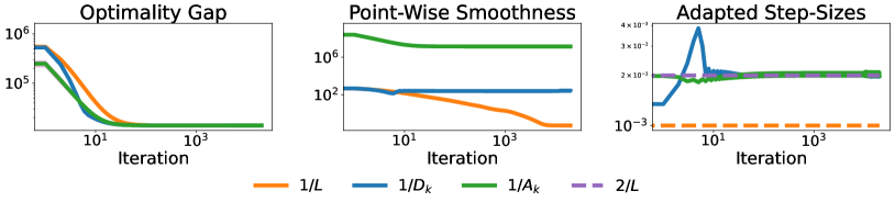
Figure 3: Performance of GD with different step-size rules for a synthetic quadratic problem. We run GD for 20,000 steps on 20 random quadratic problems with $L=1000$ and Hessian skew. Left-to-right, the first plot shows the optimality gap $f(x_{k})-f(x^{*})$, the second shows the point-wise directional smoothness, and the third shows step-sizes used by the different methods.

4.2 Adaptivity for Convex Functions

In the last subsection, we proved that strongly adapted step-sizes for the point-wise and path-wise directional smoothness functions have closed-form expressions when $f$ is quadratic. Moreover, these step-sizes recover two classical schemes from the optimization literature, giving them new justification and fast convergence rates. Now we consider the existence of strongly adapted step-sizes for general convex functions. Our first result gives simple conditions for Equation 18 to have at least one solution when $M$ is the point-wise directional smoothness.

Proposition 4.1.

If $f$ is convex and continuously differentiable, then either (i) $f$ is minimized along the ray $x(\eta)=x-\eta\nabla f(x)$ or (ii) there exists $\eta>0$ for which $\eta=1/D(x-\eta\nabla f(x),x)$ holds.

Convexity of $f$ implies the directional derivative is monotone increasing along $\nabla f(x)$, which we use to show the point-wise smoothness is well-defined for sufficiently large $\eta$. This allows us to prove existence of a strongly adapted step-size. The next proposition uses a similar argument to show existence of strongly adapted step-sizes for the path-wise smoothness under twice differentiability of $f$.

Proposition 4.2.

If $f$ is convex and twice continuously differentiable, then either (i) $f$ is minimized along the ray $x(\eta)=x-\eta\nabla f(x)$ or (ii) there exists $\eta>0$ for which $\eta=1/A(x-\eta\nabla f(x),x)$ holds.

Proposition 4.1 and Proposition 4.2 do not assume the existence of a global smoothness constant $L$, meaning both hold for functions with potentially unbounded global smoothness. Although neither proof is not constructive, it is possible to compute strongly adapted step-sizes for the point-wise directional smoothness using root-finding methods. If $f$ is twice differentiable, then strongly adapted step-sizes can be found via Newton’s method using only Hessian-vector products, $\nabla^{2}f(x)\nabla f(x)$. We experiment with this in Section 5.

4.2.1 Exponential Search

Now we show that the exponential search algorithm developed by Carmon & Hinder (2022) can be used to find step-sizes that adapt on average to the directional smoothness. Consider a fixed optimization horizon $k$ and denote by $x_{i}(\eta)$ the sequence of iterates obtained by running GD from $x_{0}$ using a fixed step-size $\eta$. Define the criterion function,

$$\psi(\eta)=\frac{\sum_{i=0}^{k}\|\nabla f(x_{i}(\eta))\|_{2}^{2}}{\sum_{i=0}^{k}M(x_{i+1}(\eta),x_{i}(\eta))\|\nabla f(x_{i}(\eta))\|_{2}^{2}},$$ (21)

and suppose that we have a step-size $\eta$ that satisfies $\psi(\eta)/2\leq\eta\leq\psi(\eta)$. Using these bounds in Proposition 3.3 yields the following convergence rate,

$$\textstyle\frac{f(\overline{x}_{k})-f_{*}}{\|x_{0}-x^{*}\|_{2}^{2}}\leq\left[\frac{k\sum_{i=0}^{k}M(x_{i+1},x_{i})\|\nabla f(x_{i})\|_{2}^{2}}{\sum_{i=0}^{k}\|\nabla f(x_{i})\|_{2}^{2}}\right].$$ (22)

We see that while the step-size $\eta$ does not adapt to each directional smoothness $M(x_{i+1},x_{i})$ along the path, it adapts to a weighted average of the directional smoothness constants, where the weights are the observed squared gradient norms. This is always smaller than the maximum directional smoothness along the trajectory, and can be much smaller than the global smoothness.

We have reduced our problem to finding $\eta\in[\psi(\eta)/2,\psi(\eta)]$, which is similar to the problem Carmon & Hinder (2022) solve with bisection. We adopt their approach as Algorithm 1. Our next theorem gives a convergence guarantee for exponential search:

Theorem 4.3.

Assume the objective $f$ is convex and $L$-smooth. Then Algorithm 1 with $\eta_{0}>0$ requires at most $2T(\log\log\frac{2\eta_{0}}{L^{-1}}\lor 1)$ iterations of GD and in the last run it outputs a step-size $\eta$ and point $\hat{x}_{T}=\frac{1}{T}\sum_{t=0}^{T-1}x_{t}(\eta)$ such that exactly one of the following holds:

$$\text{Case 1: }\quad\eta=\eta_{0}\quad\text{ and }\leq\frac{\|x_{0}-x_{*}\|_{2}^{2}}{2T\eta_{0}}$$

$$\text{Case 2: }\quad\eta\neq\eta_{0}\quad\text{ and }\quad$$

$$f(\hat{x}_{T})-f_{*}\leq\frac{\|x_{0}-x_{*}\|_{2}^{2}}{2T}\left[\frac{\sum_{i=0}^{k}M_{i}\|\nabla f(x_{i}^{\prime})\|_{2}^{2}}{\sum_{i=0}^{k}\|\nabla f(x_{i}^{\prime})\|_{2}^{2}}\right],$$

where $M_{i}\overset{\text{def}}{=}M(x_{i+1}^{\prime},x_{i}^{\prime})$ and $x_{1}^{\prime},x_{2}^{\prime},\ldots$ are the iterates generated by GD with step-size $\eta^{\prime}$ satisfying $\eta^{\prime}\in\left[\eta,2\eta\right]$.

Theorem 4.3 requires $f$ to be $L$-smooth, but has only a $\log\log$ dependence on the global smoothness constant while obtaining a convergence rate that scales with the weighted average of the directional smoothness constants along a very close trajectory $x_{1}^{\prime},x_{2}^{\prime},\ldots$. In the next section, we alleviate this weakness and give convergence bounds that depend on the unweighted average of the directional smoothness constants along the actual optimization trajectory.

4.2.2 Polyak’s Step-Size Rule and Normalized Gradient Descent

In general, it is not computationally efficient to solve a root-finding problem at every iteration of GD. Exponential search is faster, but has a double-loop structure that makes it less practical than single-loop algorithms. Our theory so-far suggests using strongly adapted step-sizes, but many other step-size selection rules exist in the literature. For example, the Polyak step-size sets

$$\eta_{k}=\gamma\frac{f(x_{k})-f(x^{*})}{{\left\lVert\nabla f(x_{k})\right\rVert}^{2}_{2}},$$ (23)

for some $\gamma>0$. The Polyak step-size is optimal for both smooth and non-smooth optimization (Hazan & Kakade, 2019), but needs the side information of $f(w^{*})$. Our next result shows that GD with the Polyak step-size achieves the same guarantee as using strongly adapted step-sizes despite using no direction smoothness information.

Theorem 4.4.

Suppose that $f$ is convex with minimizer $x^{*}$ and let $M$ be any directional smoothness function for $f$. Then GD with the Polyak step-size and $\gamma\in\left(1,2\right)$ satisfies

$$f(\overline{x})-f^{*}\leq\frac{c(\gamma){\left\lVert x_{0}-x^{*}\right\rVert}^{2}_{2}}{2\sum_{k=0}^{t-1}M(x_{k+1},x_{k})^{-1}},$$ (24)

where $c(\gamma)=\gamma/(2-\gamma)(\gamma-1)$ and,

$$\overline{x}_{t}=\frac{\sum_{k=0}^{t-1}\left[M(x_{k+1},x_{k})^{-1}x_{k}\right]}{\sum_{k=0}^{t-1}M(x_{k+1},x_{k})^{-1}}.$$ (25)

Theorem 4.4 measures sub-optimality at an average iterate obtained using the directional smoothness. However, it also holds for the best iterate, $\hat{x}=\mathop{\rm arg\,min}_{k}f(x_{k})$, so that no knowledge of the directional smoothness is required to obtain the guarantee.

Now we compare Theorem 4.4 with the standard guarantee for the Polyak step-size under $L$-smoothness (Hazan & Kakade, 2019), which states

$$f(\hat{x}_{T})-f^{*} \leq\frac{2L{\left\lVert x_{0}-x^{*}\right\rVert}^{2}_{2}}{T}.$$ (26)

Specializing Theorem 4.4 with $\gamma=1.5$, yields

$$f(\hat{x}_{T})-f^{*} \leq\frac{3{\left\lVert x_{0}-x^{*}\right\rVert}^{2}_{2}}{\sum_{k=0}^{T-1}M(x_{k+1},x_{k})^{-1}}$$

$$=\frac{3{\left\lVert x_{0}-x^{*}\right\rVert}^{2}_{2}}{T}\frac{1}{\frac{1}{T}\sum_{k=0}^{T-1}M(x_{k+1},x_{k})^{-1}}.$$

Setting $M(x_{k+1},x_{k})=L$, we immediately recover the convergence of Polyak’s method up to a $1.5$ constant factor. However, in the case that $M(x_{k+1},x_{k})\neq L$, we can potentially do much better. By Jensen’s inequality, we have

$$\frac{1}{\frac{1}{T}\sum_{k=0}^{T-1}M(x_{k+1},x_{k})^{-1}}\leq\frac{\sum_{k=0}^{T-1}M(x_{k+1},x_{k})}{T}.$$ (27)

Equation 27 shows that the convergence of the method depends on the average directional smoothness along the trajectory rather than $L$. Moreover, Theorem 4.4 applies to any convex $f$, even in the absence of global smoothness.

Comparison with strongly adapted step-sizes. As we saw for quadratics, strongly adapted step-sizes for any directional smoothness function allow us to obtain the following convergence rate:

$$f(\overline{x}_{t})-f(x^{*}) \leq\frac{{\left\lVert x_{0}-x^{*}\right\rVert}^{2}_{2}}{2\sum_{i=0}^{t-1}M(x_{i+1},x_{i})^{-1}}.$$

This is the same as the guarantee given by Equation 24 up to constant factors. As a result, we give a positive answer to our main question posed earlier in this section: GD with the Polyak step-sizes achieves the same progress in aggregate for any directional smoothness $M$ as running GD with step-sizes strongly adapted to $M$.

Application to the optimal directional smoothness. Theorem 4.4 holds for every directional smoothness function $M$. Therefore we can specialize Equation 24 with the optimal point-wise directional smoothness $H$ (as defined in Equation 5) and $\gamma=1.5$ to get the guarantee,

$$\min_{k\in[T-1]}\left[f(x_{k})-f^{*}\right]\leq\frac{3{\left\lVert x_{0}-x^{*}\right\rVert}^{2}_{2}}{\sum_{k=0}^{T-1}H(x_{k+1},x_{k})^{-1}}.$$ (28)

This rate requires computing the iterate with the minimum function value, but that is easy to track during optimization. Unlike our previous results, Equation 28 requires no access to the optimal point-wise smoothness, yet obtains a dependence on the tightest constant possible.

Now we change directions slightly and provide another algorithm whose convergence depends on the directional smoothness. The normalized GD method uses step-sizes which are normalized by the gradient magnitude,

$$x_{k+1}=x_{k}-\frac{\eta_{k}}{\|\nabla f(x_{k})\|_{2}}\nabla f(x_{k}).$$ (29)

Our next theorem shows that normalized GD obtains a guarantee which depends solely on the average of the point-wise directional smoothness $D(x_{k},x_{k+1})$ encountered along the trajectory despite no explicit knowledge of the smoothness.

Theorem 4.5.

Suppose that $f$ is convex with minimizer $x^{*}$. Let $D$ be the point-wise directional smoothness defined by Equation 5 and $\Delta_{0}:=\|x_{0}-x_{*}\|_{2}^{2}$. Then normalized GD with a sequence of non-increasing step-sizes $\eta_{k}$ satisfies

$$\begin{split}&f(\hat{x})-f^{*}\leq\frac{\Delta_{0}^{2}+\sum_{t=0}^{T-1}\eta_{t}^{2}}{2T^{2}}\left(\frac{f(x_{0})}{\eta_{0}^{2}}-\frac{f^{*}}{\eta_{T-1}^{2}}\right)\\ &\hskip 20.00003pt+\frac{\Delta_{0}^{2}+\sum_{t=0}^{T-1}\eta_{t}^{2}}{2T}\sum_{t=0}^{T-1}\frac{M(x_{t},x_{t+1})}{T},\end{split}$$ (30)

where $\hat{x}=\arg\min_{k}f(x_{k})$. Consequently, for $\eta_{t}=1/\sqrt{T}$ we have $f(\hat{x})-f^{*}=\mathcal{O}(1/T)$ and for $\eta_{t}=1/\sqrt{t}$ we get the anytime result $f(\hat{x})-f^{*}=\mathcal{O}(\log(t)/t).$

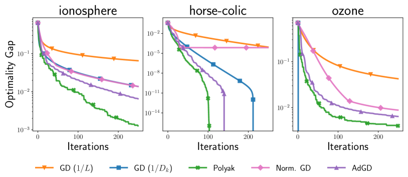
Figure 4: Comparison of GD with the optimal fixed step-size ($\eta_{k}=1/L$), step-sizes strongly adapted to the point-wise smoothness ($\eta_{k}=1/D(x_{k+1},x_{k})$), and the Polyak step-size against normalized GD (Norm. GD) and the AdGD method on three logistic regression problems. AdGD uses a smoothed version of the point-wise directional smoothness from the previous iteration to set the step-size. We find that GD methods with adaptive step-sizes consistently outperform GD with $\eta=1/L$ and even obtain a linear rate on horse-colic.

Theorem 4.5 gives a rate for normalized GD which is valid for any convex function $f$ and does not depend on any global smoothness constants. It does not, however, match the better guarantee achieved by GD with Polyak step-sizes.

5 Experiments

We evaluate the practical improvement of our convergence rates over those based on $L$-smoothness using two logistic regression problems taken from the UCI repository (Asuncion & Newman, 2007). Figure 1 compares GD with strongly adapted step-sizes $\eta=\frac{1}{M_{k}}$, where $M_{k}$ is taken to be the point-wise smoothness, against GD with the Polyak step-size. We also plot the exact convergence rates for each method, Equation 17 and Equation 24, respectively, and compare against the classical guarantee for both methods. Our convergence rates are an order of magnitude tighter on the ionosphere dataset and display a remarkable ability to adapt to the path of optimization on mammographic.

Figure 3 compares the performance of GD with strongly adapted step-sizes and with the fixed step-size $\eta_{k}=1/L$ for a synthetic quadratic with Hessian skew (Pan et al., 2022). Results are averaged over twenty random problems. We find that strongly adapted step-sizes lead to significantly faster optimization. Since $A_{k},D_{K}\ll L$, the adapted step-sizes are larger than $2/L$, especially at the start of training; they eventually converge to $2/L$, indicating these methods operate at the edge-of-stability (Cohen et al., 2021, 2022).

Finally, we conclude with a comparison of empirical convergence rates on three additional logistic regression problems from the UCI repository. We compare GD with $\eta_{k}=1/L$, GD with step-sizes strongly adapted to the point-wise smoothness ($\eta_{k}=1/D_{k}$), GD with the Polyak step-size (Polyak), and normalized GD (Norm. GD) against the AdGD method (Malitsky & Mishchenko, 2020). The Polyak step-size performs best on every dataset but ozone, where GD with $\eta_{k}=1/D_{k}$ solves the problem to high accuracy in just a few iterations. Thus, although Polyak step-sizes have the optimal dependence on directional smoothness, computing strongly adapted step-sizes can still be advantageous.

6 Conclusion

We present new sub-optimality bounds for GD under novel measures of local gradient variation which we call directional smoothness functions. Our results hold for any sequence of step-sizes, improve over standard analyses when $\eta_{k}$ is adapted to the choice of directional smoothness function, and depend only on properties of $f$ local to the optimization path. For convex quadratics, we show that computing step-sizes which are strongly adapted to directional smoothness functions is straightforward and recovers two well-known step-size schemes, one of which is the Cauchy step-size. In the general case, we prove that an algorithm based on exponential search gives a weighted-version of the path-dependent convergence rate with no need for adapted step-sizes. We also show that GD with the Polyak step-size and normalized GD both obtain fast rates with no dependence on the global smoothness parameter, $L$. The Polyak step-size, in particular, adapts to any choice of directional smoothness, including the tightest possible parameter.

Broader Impacts

This paper presents work whose goal is to advance the field of Machine Learning. There are many potential societal consequences of our work, none which we feel must be specifically highlighted here.

Appendix A Proofs for Section 2

See 2.2

Proof.

By the convexity of $f$ we have

$$f(x)+\left\langle\nabla f(x),y-x\right\rangle\leq f(y).$$

Rearranging and then using Cauchy-Schwarz we get

$$f(x) \leq f(y)+\left\langle\nabla f(x),x-y\right\rangle$$

$$=f(y)+\left\langle\nabla f(y),x-y\right\rangle+\left\langle\nabla f(x)-\nabla f(y),x-y\right\rangle$$

$$\leq f(y)+\left\langle\nabla f(y),x-y\right\rangle+\|\nabla f(x)-\nabla f(y)\|\|x-y\|$$

$$=f(y)+\left\langle\nabla f(y),x-y\right\rangle+\frac{D(x,y)}{2}\|x-y\|^{2}.\qed$$

See 2.4

Proof.

Starting from the fundamental theorem of calculus,

$$f(x)-\left\langle\nabla f(x),y-x\right\rangle =\int_{0}^{1}\left\langle\nabla f(x+t(y-x))-\nabla f(x),y-x\right\rangle dt$$

$$\leq\int_{0}^{1}A(x,y)t\|x-y\|_{2}^{2}dt$$

$$=\frac{A(x,y)}{2}\|y-x\|^{2}_{2}.$$

which completes the proof. ∎

See 2.3

Proof.

Let $H_{f}$ denote the optimal pointwise directional smoothness associated with some convex and differentiable function $f:\mathbb{R}^{d}\rightarrow\mathbb{R}$ (as defined in Equation 5), and $D_{f}$ denote the pointwise directional smoothness associated with $f$ (as defined in Equation 5). For any $t$, statement of (7) is equivalent to saying $H_{f}\leq t\frac{\|\nabla f(x)-\nabla f(y)\|}{\|x-y\|}$ for all $x,y\in\mathbb{R}^{d}$ and convex, differentiable $f$. Observe that Lemma 2.2 already shows that for all convex and differentiable functions $f:\mathbb{R}^{d}\rightarrow\mathbb{R}$

$$H_{f}(x,y)\leq D_{f}(x,y)=2\frac{\|\nabla f(x)-\nabla f(y)\|}{\|x-y\|}$$

for all $x,y\in\mathbb{R}^{d}$. In order to show that this is tight, we suppose by the way of contradiction that there exists some $2>t\geq 0$ such that for all convex and differentiable functions $f:\mathbb{R}^{d}\rightarrow\mathbb{R}$

$$H_{f}(x,y)\leq t\cdot\frac{\|\nabla f(x)-\nabla f(y)\|}{\|x-y\|}$$ (31)

for all $x,y\in\mathbb{R}$. We shall show that no such $t$ exists by showing for each such $t$ there exists a function $f_{t}$ such that Equation 31 does not hold.

Consider $f_{\epsilon}(x)=\sqrt{x^{2}+\epsilon^{2}}$ for $\epsilon\leq 1$. The function $f$ is differentiable. Moreover

$$f_{\epsilon}^{\prime}(x)=\frac{x}{\sqrt{x^{2}+\epsilon^{2}}}, f_{\epsilon}^{\prime\prime}(x)=\frac{\epsilon^{2}}{(\epsilon^{2}+x^{2})^{\frac{3}{2}}}\geq 0.$$

Therefore $f$ is convex. Let $g(x)=\left|x\right|$. Fix $x=1$ and $y=0$, we have

$$\begin{split}\left|g(x)-g(y)-{\text{sign}(y)\cdot(x-y)}\right|&\leq\left|f_{\epsilon}(x)-f_{\epsilon}(y)-{f_{\epsilon}^{\prime}(y)\cdot(x-y)}\right|\\ &\qquad+\left|g(x)-f_{\epsilon}(x)\right|+\left|g(y)-f_{\epsilon}(y)\right|+\left|{(f_{\epsilon}^{\prime}(y)-\text{sign}(y))\cdot(x-y)}\right|\end{split}$$

$$\begin{split}&=\left|f_{\epsilon}(x)-f_{\epsilon}(y)-{f_{\epsilon}^{\prime}(y)\cdot(x-y)}\right|+\left|1-\sqrt{1+\epsilon^{2}}\right|+\left|0-\sqrt{\epsilon^{2}}\right|+\left|(0-0)\cdot(1-0)\right|\\ &\leq\left|f_{\epsilon}(x)-f_{\epsilon}(y)-{f_{\epsilon}^{\prime}(y)\cdot(x-y)}\right|+2\epsilon.\end{split}$$

Now observe that

$$g(x)-g(y)-{\text{sign}(y)\cdot(x-y)} =\left|1\right|-\left|0\right|-0\cdot(1-0)=1.$$

Therefore

$$\left|f_{\epsilon}(x)-f_{\epsilon}(y)-{f_{\epsilon}^{\prime}(y)\cdot(x-y)}\right|\geq 1-2\epsilon.$$ (32)

By definition we have $\frac{1}{2}{\left\lVert x-y\right\rVert}^{2}=\frac{1}{2}$, therefore

$$H_{f}(x,y)\;=\;\frac{\left|f_{\epsilon}(x)-f_{\epsilon}(y)-{f_{\epsilon}^{\prime}(y)\cdot(x-y)}\right|}{\frac{1}{2}{\left\lVert x-y\right\rVert}^{2}}\geq 2-4\epsilon.$$ (33)

But by our starting assumption we have that there exists some $t<2$ such that $H_{f}(x,y)\leq t\frac{\|f^{\prime}(x)-f^{\prime}(y)\|}{\left|x-y\right|}$ for all differentiable and convex functions $f$. Applying this to $f=f_{\epsilon}$ we get

$$H_{f_{\epsilon}}(1,0) \leq t\frac{\left|f_{\epsilon}^{\prime}(1)-f_{\epsilon}^{\prime}(0)\right|}{\left|1\right|}=t\cdot\frac{1}{\sqrt{1+\epsilon^{2}}}\leq t.$$ (34)

Combining Equations 33 and 34 we have

$$2-4\epsilon\leq H_{f_{\epsilon}}(1,0)\leq t$$

Rearranging we get

$$2-t\leq 4\epsilon$$

Choosing $\epsilon=\frac{2-t}{8}>0$ we get a contradiction. It follows that the minimal $t$ such that $H(x,y)\leq t\frac{\left|f^{\prime}(x)-f^{\prime}(y)\right|}{\left|x-y\right|}$ for all convex and differentiable $f$ is $t=2$. ∎

Lemma A.1.

One step of gradient descent with step-size $\eta_{k}>0$ makes progress as

$$f(x_{k+1})\leq f(x_{k})-\eta_{k}\left(1-\frac{\eta_{k}M(x_{k+1},x_{k})}{2}\right)\|\nabla f(x_{k})\|_{2}^{2}.$$

Proof.

Starting from Equation 5, we have

$$f(x_{k+1}) \leq f(x_{k})+\left\langle\nabla f(x_{k}),x_{k+1}-x_{k}\right\rangle+\frac{M(x_{k+1},x_{k})}{2}\|x_{k+1}-x_{k}\|_{2}^{2}$$

$$=f(x_{k})-\eta_{k}\|\nabla f(x_{k})\|_{2}^{2}+\frac{\eta_{k}^{2}M(x_{k+1},x_{k})}{2}\|\nabla f(x_{k})\|_{2}^{2}$$

$$=f(x_{k})-\eta_{k}\left(\frac{1-\eta_{k}M(x_{k+1},x_{k})}{2}\right)\|\nabla f(x_{k})\|_{2}^{2}.$$

∎

Appendix B Proofs for Section 3

Lemma B.1.

If $f$ is convex, then for any $y,x\in\mathbb{R}^{d}$,

$$f(y)\geq f(x)+\left\langle\nabla f(x),y-x\right\rangle+\frac{\mu(y,x)}{2}\|y-x\|_{2}^{2}.$$ (35)

If $f$ is $\mu$ strongly convex, then $\mu(y,x)\geq\mu$.

Proof.

The fundamental theorem of calculus implies

$$f(x)-\left\langle\nabla f(x),y-x\right\rangle =\int_{0}^{1}\left\langle\nabla f(x+t(y-x))-\nabla f(x),y-x\right\rangle dt$$

$$\geq\int_{0}^{1}\mu(x,y)t\|x-y\|_{2}^{2}dt$$

$$=\frac{\mu(x,y)}{2}\|y-x\|^{2}_{2}.$$

Note that we have implicitly used convexity to verify the inequality in the second line in the case where $\mu(y,x)=0$. Now assume that $f$ is $\mu$ strongly convex. As a standard consequence of strong-convexity, we obtain:

$$\frac{\left\langle\nabla f(x+t(y-x))-\nabla f(x),y-x\right\rangle}{t\|x-y\|_{2}^{2}} =\frac{\left\langle\nabla f(x+t(y-x))-\nabla f(x),x+t(y-x)-x\right\rangle}{t^{2}\|x-y\|_{2}^{2}}$$

$$\geq\mu\frac{\|x-t(y-x)-x\|_{2}^{2}}{t^{2}\|y-x\|_{2}^{2}}$$

$$=\mu.$$

∎

See 3.1

Proof.

First note that $\lambda_{i}<0$ for $i\in\mathcal{G}$ and $\lambda_{i}\geq 0$ for $i\in\mathcal{B}$. We start from Equation 11,

$$f(x_{k+1}) \leq f(x_{k})+\eta_{k}\left(\frac{\eta_{k}M(x_{k+1},x_{k})}{2}-1\right)\|\nabla f(x_{k})\|_{2}^{2}$$

$$=f(x_{k})+\mathbbm{1}_{k\in\mathcal{G}}\cdot\left[\frac{\eta_{k}\lambda_{k}}{2}\|\nabla f(x_{k})\|_{2}^{2}\right]+\mathbbm{1}_{k\in\mathcal{B}}\cdot\left[\frac{\eta_{k}\lambda_{k}}{2}\|\nabla f(x_{k})\|_{2}^{2}\right]$$

$$\leq f(x_{k})+\mathbbm{1}_{k\in\mathcal{G}}\cdot\left[\eta_{k}\lambda_{k}\mu_{k}\left(f(x_{k})-f(x^{*})\right)\right]+\mathbbm{1}_{k\in\mathcal{B}}\cdot\left[\frac{\eta_{k}\lambda_{k}}{2}\|\nabla f(x_{k})\|_{2}^{2}\right],$$

where we used that directional strong convexity gives

$$\|\nabla f(x_{k})\|_{2}^{2}\geq 2\mu_{k}\left(f(x_{k})-f(x^{*})\right).$$

Subtracting $f(x^{*})$ from both sides and then recursively applying the inequality gives the result. ∎

See 3.2

Proof.

Let $\Delta_{k}=\|x_{k}-x^{*}\|_{2}^{2}$ and observe

$$\Delta_{k}=\|x_{k}-x_{k+1}+x_{k+1}-x^{*}\|_{2}^{2}=\Delta_{k+1}+\|x_{k}-x_{k+1}\|_{2}^{2}+2\left\langle x_{k}-x_{k+1},x_{k+1}-x^{*}\right\rangle.$$

Using this expansion in $\Delta_{k+1}-\Delta_{k}$, we obtain

$$\Delta_{k+1}-\Delta_{k} =-\|x_{k}-x_{k+1}\|_{2}^{2}-2\left\langle x_{k}-x_{k+1},x_{k+1}-x^{*}\right\rangle$$

$$=-\eta_{k}^{2}\|\nabla f(x_{k})\|_{2}^{2}-2\eta_{k}\left\langle\nabla f(x_{k}),x_{k+1}-x^{*}\right\rangle$$

$$=-\eta_{k}^{2}\|\nabla f(x_{k})\|_{2}^{2}-2\eta_{k}\left\langle\nabla f(x_{k}),x_{k+1}-x_{k}\right\rangle-2\eta_{k}\left\langle\nabla f(x_{k}),x_{k}-x^{*}\right\rangle.$$

Now we control the inner-products with directional strong convexity and directional smoothness.

$$\leq-\eta_{k}^{2}\|\nabla f(x_{k})\|_{2}^{2}-2\eta_{k}\left\langle\nabla f(x_{k}),x_{k+1}-x_{k}\right\rangle+2\eta_{k}\left[f(x^{*})-f(x_{k})-\frac{\mu_{k}}{2}\Delta_{k}\right]$$

$$\leq-\eta_{k}^{2}\|\nabla f(x_{k})\|_{2}^{2}+2\eta_{k}\left[f(x_{k})-f(x_{k+1})+\frac{M(x_{k+1},x_{k})\eta_{k}^{2}}{2}\|\nabla f(x_{k})\|\right]$$

$$\qquad+2\eta_{k}\left[f(x^{*})-f(x_{k})-\frac{\mu_{k}}{2}\Delta_{k}\right]$$

$$=\eta_{k}^{2}\left(M(x_{k+1},x_{k})\eta_{k}-1\right)\|\nabla f(x_{k})\|_{2}^{2}+2\eta_{k}\left[f(x^{*})-f(x_{k+1})\right]-\mu_{k}\eta_{k}\Delta_{k}$$

$$\leq\eta_{k}^{2}\left(M(x_{k+1},x_{k})\eta_{k}-1\right)\|\nabla f(x_{k})\|_{2}^{2}-\mu_{k}\eta_{k}\Delta_{k}.$$

Re-arranging this expression allows us to deduce a rate with error terms depending on the local smoothness,

$$\implies\Delta_{k+1} \leq\left(1-\mu_{k}\eta_{k}\right)\Delta_{k}+\eta_{k}^{2}\left(M(x_{k+1},x_{k})\eta-1\right)\|\nabla f(x_{k})\|_{2}^{2}$$

$$\leq\left[\prod_{i=0}^{k}\left(1-\mu_{i}\eta_{i}\right)\right]\Delta_{0}+\sum_{i=0}^{k}\left[\prod_{j=i+1}^{k}\left(1-\mu_{j}\eta_{j}\right)\right]\eta_{i}^{2}\left(M(x_{i+1},x_{i})\eta_{i}-1\right)\|\nabla f(x_{i})\|_{2}^{2}.$$

∎

See 3.3

Proof.

Let $\Delta_{k}=\|x_{k}-x^{*}\|_{2}^{2}$ and observe

$$\Delta_{k}=\|x_{k}-x_{k+1}+x_{k+1}-x^{*}\|_{2}^{2}=\Delta_{k+1}+\|x_{k}-x_{k+1}\|_{2}^{2}+2\left\langle x_{k}-x_{k+1},x_{k+1}-x^{*}\right\rangle.$$

Using this expansion in $\Delta_{k+1}-\Delta_{k}$, we obtain

$$\Delta_{k+1}-\Delta_{k} =-\|x_{k}-x_{k+1}\|_{2}^{2}-2\left\langle x_{k}-x_{k+1},x_{k+1}-x^{*}\right\rangle$$

$$=-\eta_{k}^{2}\|\nabla f(x_{k})\|_{2}^{2}-2\eta_{k}\left\langle\nabla f(x_{k}),x_{k+1}-x^{*}\right\rangle$$

$$=-\eta_{k}^{2}\|\nabla f(x_{k})\|_{2}^{2}-2\eta_{k}\left\langle\nabla f(x_{k}),x_{k+1}-x_{k}\right\rangle-2\eta_{k}\left\langle\nabla f(x_{k}),x_{k}-x^{*}\right\rangle.$$

Now we use convexity and directional smoothness to control the two inner-products as follows:

$$\Delta_{k+1}-\Delta_{k} \leq-\eta_{k}^{2}\|\nabla f(x_{k})\|_{2}^{2}-2\eta_{k}\left(f(x_{k})-f(x^{*})\right)-2\eta_{k}\left\langle\nabla f(x_{k}),x_{k+1}-x_{k}\right\rangle$$

$$\leq-\eta_{k}^{2}\|\nabla f(x_{k})\|_{2}^{2}-2\eta_{k}\left(f(x_{k})-f(x^{*})\right)+2\eta_{k}(f(x_{k})-f(x_{k+1}))+\eta_{k}^{3}M(x_{k+1},x_{k})\|\nabla f(x_{k})\|_{2}^{2}$$

$$=\eta_{k}^{2}(\eta_{k}M(x_{k+1},x_{k})-1)\|\nabla f(x_{k})\|_{2}^{2}-2\eta_{k}\left(f(x_{k+1})-f(x^{*})\right).$$

Re-arranging this equation and summing over iterations implies the following sub-optimality bound:

$$\sum_{i=0}^{k}\frac{\eta_{i}}{\sum_{i=0}^{k}\eta_{i}}\left(f(x_{i+1})-f(x^{*})\right) \leq\frac{\Delta_{0}+\sum_{i=0}^{k}\eta_{i}^{2}(\eta_{i}M(x_{i+1},x_{i})-1)\|\nabla f(x_{i})\|_{2}^{2}}{2\sum_{i=0}^{k}\eta_{i}}.$$

Convexity of $$f$$ and Jensen’s inequality now imply the final result,

$$\implies f(\overline{x}_{k})-f(x^{*}) \leq\frac{\Delta_{0}+\sum_{i=0}^{k}\eta_{i}^{2}(\eta_{i}M(x_{i+1},x_{i})-1)\|\nabla f(x_{i})\|_{2}^{2}}{2\sum_{i=0}^{k}\eta_{i}}.$$

∎

Appendix C Proofs for Section 4.1

Lemma C.1.

Let $B$ be a positive semi-definite matrix and suppose that

$$f(x)=\frac{1}{2}x^{\top}Bx-c^{\top}x.$$

Let $x_{i+1}=x_{i}-\eta\nabla f(x_{i})$. Then for any $\eta>0$, the pointwise directional smoothness between the gradient descent iterates $x_{i},x_{i+1}$ is given by

$$\frac{1}{2}D(x_{i+1},x_{i})=\frac{\|B\nabla f(x_{i})\|}{\|\nabla f(x_{i})\|}.$$

Proof.

We have by straightforward algebra,

$$\frac{1}{2}D(x_{i+1},x_{i}) =\frac{\|\nabla f(x_{i+1})-\nabla f(x_{i})\|}{\|x_{i+1}-x_{i}\|}$$

$$=\frac{\|\left[Bx_{i+1}-c\right]-\left[Bx_{i}-c\right]\|}{x_{i+1}-x_{i}}$$

$$=\frac{\|B\left[x_{i+1}-x_{i}\right]\|}{x_{i+1}-x_{i}}$$

$$=\frac{\|B\left[-\eta\nabla f(x_{i})\right]\|}{\|-\eta\nabla f(x_{i})\|}$$

$$=\frac{\|B\nabla f(x_{i})\|}{\|\nabla f(x_{i})\|}.$$

∎

Lemma C.2.

Let $B$ be a positive semi-definite matrix and suppose that

$$f(x)=\frac{1}{2}x^{\top}Bx-c^{\top}x.$$

Let $x_{i+1}=x_{i}-\eta\nabla f(x_{i})$. Then for any $\eta>0$, the path-wise directional smoothness between the gradient descent iterates $x_{i},x_{i+1}$ is given by by

$$A(x_{i+1},x_{i})=\frac{{\nabla f(x_{i})^{\top}B\nabla f(x_{i})}}{\nabla f(x_{i})^{\top}\nabla f(x_{i})}.$$

Proof.

Let $A_{t}(x,y)=\frac{\left\langle\nabla f(x+t(y-x))-\nabla f(x),y-x\right\rangle}{t{\left\lVert x-y\right\rVert}^{2}}$. We have

$$A_{t}(x,y) =\frac{\left\langle\nabla f(x+t(y-x))-\nabla f(x),y-x\right\rangle}{t{\left\lVert x-y\right\rVert}^{2}}$$

$$=\frac{\left\langle(B(x+t(y-x)))-c-\left[Bx-c\right],y-x\right\rangle}{t{\left\lVert x-y\right\rVert}^{2}}$$

$$=\frac{\left\langle t\cdot B(y-x),y-x\right\rangle}{t{\left\lVert x-y\right\rVert}^{2}}$$

$$=\frac{(y-x)^{\top}B(y-x)}{{\left\lVert x-y\right\rVert}^{2}}.$$

The path-wise directional smoothness $A$ is therefore

$$A(x,y) =\sup_{t\in[0,1]}A_{t}(x,y)$$

$$=\sup_{t\in[0,1]}\frac{(y-x)^{\top}B(y-x)}{{\left\lVert x-y\right\rVert}^{2}}$$

$$=\frac{(y-x)^{\top}B(y-x)}{{\left\lVert x-y\right\rVert}^{2}}.$$

Plugging in $y=x-\eta\nabla f(x)=x-\eta[Bx-c]$ in the above gives

$$A(x-\eta\nabla f(x),x) =\frac{\left(-\eta\left[Bx-c\right]\right)B(-\eta)\left[Bx-c\right]}{{\left\lVert\eta[Bx-c]\right\rVert}^{2}}$$

$$=\frac{(Bx-c)^{\top}B(Bx-c)}{{\left\lVert Bx-c\right\rVert}^{2}}$$

$$=\frac{(Bx-c)^{\top}B(Bx-c)}{{\left\lVert Bx-c\right\rVert}^{2}}$$

$$=\frac{\nabla f(x)^{\top}B\nabla f(x)}{\nabla f(x)^{\top}\nabla f(x)}.$$

∎

Appendix D Proofs for Section 4.2

See 4.1

Proof.

Let $\mathcal{I}=\left\{\eta:\nabla f(x-\eta\nabla f(x))=\nabla f(x)\right\}$. For every $\eta\in\mathcal{I}$, it holds that

$$-\left\langle\nabla f(x-\eta\nabla f(x)),\nabla f(x)\right\rangle=-\|\nabla f(x)\|_{2}^{2}.$$

However, since $f$ is convex, the directional derivative

$$-\left\langle\nabla f(x-\eta^{\prime}\nabla f(x)),\nabla f(x)\right\rangle,$$

is monotone non-decreasing in $\eta^{\prime}$. We deduce that $\mathcal{I}$ must be an interval of form $[0,\overline{\eta}]$. If $\overline{\eta}$ is not bounded, then $f$ is linear along $-\nabla f(x)$ and is minimized by taking $\eta\rightarrow\infty$. Therefore, we may assume $\overline{\eta}$ is finite.

Let $\eta>\overline{\eta}$. Then we have the following:

$$x-\eta\nabla f(x) =x-\frac{2\|x-\eta\nabla f(x)-x\|_{2}}{\|\nabla f(x-\eta\nabla f(x))-\nabla f(x)\|_{2}}\nabla f(x)$$

$$\implies\nabla f(x) =\frac{2\|\nabla f(x)\|_{2}}{\|\nabla f(x-\eta\nabla f(x))-\nabla f(x)\|_{2}}\nabla f(x),$$

from which we deduce

$$\|\nabla f(x-\eta\nabla f(x))-\nabla f(x)\|_{2}=2\|\nabla f(x)\|_{2},$$

is sufficient for the implicit equation to hold. Squaring both sides and multiplying by $1/2$, we obtain the following alternative root-finding problem:

$$h(\eta):=\frac{1}{2}\|\nabla f(x-\eta\nabla f(x))\|_{2}^{2}-\left\langle\nabla f(x-\eta\nabla f(x)),\nabla f(x)\right\rangle-\frac{1}{2}\|\nabla f(x)\|_{2}^{2}=0.$$ (36)

Because $f$ is $C^{1}$, $h$ is a continuous function and it suffices to show that there exists an interval in which $h$ crosses $0$. From the display above, we see

$$h(\overline{\eta})=-\|\nabla f(x)\|_{2}^{2}<0.$$

Continuity now implies $\exists\eta^{\prime}>\overline{\eta}$ such that $h(\eta^{\prime})<0$. Now, suppose $h(\eta)\leq 0$ for all $\eta\geq\eta^{\prime}$. Working backwards, we see that this can only occur when

$$\eta\leq\frac{2\|x-\eta\nabla f(x)-x\|_{2}}{\|\nabla f(x-\eta\nabla f(x))-\nabla f(x)\|_{2}}=\frac{1}{M(x-\eta\nabla f(x),x(\eta))}$$

for all $\eta\geq\eta^{\prime}$. The directional descent lemma (Equation 11) now implies

$$f(x-\eta\nabla f(x))\leq f(x)-\eta\left(1-\frac{\eta M(x-\eta\nabla f(x),x)}{2}\right)\|\nabla f(x)\|_{2}^{2}\leq f(x)-\frac{\eta}{2}\|\nabla f(x)\|_{2}^{2},$$

Taking limits on both sides as $\eta\rightarrow\infty$ implies $f(x-\eta\nabla f(x))$ is minimized along the ray $x(\eta)=x-\eta\nabla f(x)$. Thus, we deduce that either there exists $\eta^{\prime\prime}>\eta^{\prime}$ such that $h(\eta^{\prime\prime})>0$ exists, or $f$ is minimized along the gradient direction as claimed. ∎

See 4.2

Proof.

Let

$$\mathcal{J}=\left\{\eta:\left\langle\nabla f(x-\eta\nabla f(x)),\nabla f(x)\right\rangle=\|\nabla f(x)\|_{2}^{2}\right\}.$$

Since $f$ is convex, the directional derivative

$$-\left\langle\nabla f(x-\eta^{\prime}\nabla f(x)),\nabla f(x)\right\rangle,$$

is monotone non-decreasing in $\eta^{\prime}$. We deduce that $\mathcal{J}$ must be an interval of form $[0,\overline{\eta}]$. If $\overline{\eta}$ is not bounded, then convexity implies

$$\lim_{\eta\rightarrow\infty}f(x-\eta\nabla f(x)) \leq\lim_{\eta\rightarrow\infty}f(x)-\eta\left\langle\nabla f(x-\eta\nabla f(x)),\nabla f(x)\right\rangle$$

$$=-\infty,$$

meaning $f$ is minimized along $-\nabla f(x)$. Therefore, we may assume $\overline{\eta}$ is finite.

We have

$$x-\eta\nabla f(x) =x-\frac{1}{A(x-\eta\nabla f(x),x)}\nabla f(x)$$

$$\iff\eta =\inf_{t\in[0,1]}\frac{t\eta\|\nabla f(x)\|_{2}^{2}}{\left\langle\nabla f(x)-\nabla f(x-t\eta\nabla f(x)),\nabla f(x)\right\rangle}.$$

Thus, for $\eta>\overline{\eta}$, the equation we must solve reduces to

$$h(\eta):=\eta-\inf_{t\in[0,1]}\frac{t\eta\|\nabla f(x)\|_{2}^{2}}{\left\langle\nabla f(x)-\nabla f(x-t\eta\nabla f(x)),\nabla f(x)\right\rangle}=0.$$

Since $f$ is $C^{2}$, $h$ is continuous (see, e.g. Hogan (1973, Theorem 7)) and it suffices to show that there exists an interval over which $h$ crosses $0$.

Using Taylor’s theorem, we can re-write this expression as

$$h(\eta) =\eta-\inf_{t\in[0,1]}\frac{\|\nabla f(x)\|_{2}^{2}}{\left\langle\nabla f(x),\nabla^{2}f(x-\alpha(t\eta)\nabla f(x))\nabla f(x)\right\rangle},$$

where for some $\alpha(t\eta)\in[0,t\eta]$. Examining the denominator, we find that,

$$\int_{0}^{t}\nabla f(x)^{\top}\nabla^{2}f(x-t\overline{\eta}\nabla f(x))\nabla f(x)dt=\left\langle\nabla f(x-\overline{\eta}\nabla f(x))-\nabla f(x),\nabla f(x)\right\rangle=0,$$

which, since $f$ is convex, implies

$$\nabla f(x)^{\top}\nabla^{2}f(x-\alpha\nabla f(x))\nabla f(x)=0,$$

for every $\alpha\in[0,\overline{\eta}]$. By continuity of the Hessian, for every $\epsilon>0$, there exists $\delta>0$ such that $\eta^{\prime}\in[\overline{\eta},\overline{\eta}+\delta]$ guarantees,

$$\nabla f(x)^{\top}\nabla^{2}f(x-\eta^{\prime}\nabla f(x))\nabla f(x)<\epsilon.$$

Substituting this into our expression for $h$,

$$h(\eta^{\prime}) =\eta^{\prime}-\inf_{t\in[0,1]}\frac{\|\nabla f(x)\|_{2}^{2}}{\left\langle\nabla f(x),\nabla^{2}f(x-\alpha(t\eta^{\prime})\nabla f(x))\nabla f(x)\right\rangle}$$

$$<\overline{\eta}+\delta-\frac{\|\nabla f(x)\|_{2}^{2}}{\epsilon}$$

$$<0,$$

for $\epsilon,\delta$ sufficiently small. Thus, there exists $\eta^{\prime}>\overline{\eta}$ for which $h(\eta^{\prime})<0$.

Now let us show that $h(\eta^{\prime\prime})>0$ for some $\eta^{\prime\prime}$. For convenience, define

$$g(\eta)=\inf_{t\in[0,1]}\frac{t\|\nabla f(x)\|_{2}^{2}}{\left\langle\nabla f(x)-\nabla f(x-t\eta\nabla f(x)),\nabla f(x)\right\rangle},$$

which is a continuous and monotone non-increasing function. Take $\eta\rightarrow\infty$ and let

$$\lim_{\eta\rightarrow\infty}g(\eta)=c,$$

where the limit exists, but may be $-\infty$. Indeed, it must hold that $c<\infty$ since,

$$\lim_{\eta\rightarrow\infty}g(\eta)<g(\eta^{\prime})<\infty.$$

If $c<0$, then taking $\eta^{\prime\prime}$ large enough that $g(\eta^{\prime\prime})\leq 0$ suffices. Alternatively, if $c\geq 0$, then there exists $\tilde{\eta}$ such that $g(\eta)\leq c+\epsilon$ for every $\eta\geq\tilde{\eta}$. Choosing $\eta^{\prime\prime}>\max\left\{\tilde{\eta},c\right\}+\epsilon$ yields

$$h(\eta^{\prime\prime})=\eta^{\prime\prime}-g(\eta^{\prime\prime})>c+\epsilon-c-\epsilon=0.$$

This completes the proof. ∎

Algorithm 1 Gradient Descent with Exponential Search

1:  Procedure ExponentialSearch($x,L_{0}$)

2:  for $k=1,2,3,\ldots$ do

3:     $\eta_{\mathrm{out}}\leftarrow(RootFindingBisection){x,2^{-2^{k}}\eta_{0},\eta_{0}}$.

4:     if $\eta_{\mathrm{out}}<\infty$ then

5:        Return $\eta_{\mathrm{out}}$

6:     end if

7:  end for

8:  End Procedure

9:  Procedure RootFindingBisection($x,\eta_{\mathrm{lo}},\eta_{\mathrm{hi}}$)

10:  Define $\phi(\eta)=\eta-\psi(\eta)$ where $\psi(\eta)$ is given in (21) $\backslash\backslash$ One access to $\phi$ requires $T$ descent steps.

11:  if $\phi(\eta_{\mathrm{hi}})\leq 0$ then

12:     Return $\eta_{\mathrm{hi}}$

13:  end if

14:  if $\phi(\eta_{\mathrm{lo}})>0$ then

15:     Return $\infty$

16:  end if

17:  while $\eta_{\mathrm{hi}}>2\eta_{\mathrm{lo}}$ do

18:     $\eta_{\mathrm{mid}}=\sqrt{\eta_{\mathrm{lo}}\eta_{\mathrm{hi}}}$

19:     if $\phi(\eta_{\mathrm{mid}})>0$ then

20:        $\eta_{\mathrm{hi}}=\eta_{\mathrm{mid}}$

21:     else

22:        $\eta_{\mathrm{lo}}=\eta_{\mathrm{mid}}$

23:     end if $\backslash\backslash$ Invariant: $\phi(\eta_{\textrm{hi}})>0$, and $\phi(\eta_{\mathrm{lo}})\leq 0$.

24:  end while

25:  Return $\eta_{\mathrm{lo}}$

26:  End Procedure

See 4.3

Proof of Theorem 4.3.

This analysis follows (Carmon & Hinder, 2022). First, instantiate Equation 17 from Proposition 3.3 with $\eta_{i}=\eta$ for all $i$ to obtain

$$f(\overline{x}_{k})-f^{*}\leq\frac{\|x_{0}-x^{*}\|^{2}}{2\eta k}+\frac{\eta\left[\eta\sum_{i=0}^{k}M(x_{i+1},x_{i})\|\nabla f(x_{i})\|^{2}-\sum_{i=0}^{k}\|\nabla f(x_{i})\|^{2}\right]}{2k}.$$ (37)

Now, observe that if we get a “Lucky strike” and $\phi(\eta_{\mathrm{hi}})=\phi(\eta_{0})\leq 0$, then specializing Equation 37 for $\eta=\eta_{0}$ we get

$$f(\overline{x}_{k})-f_{\ast} \leq\frac{{\left\lVert x_{0}-x_{\ast}\right\rVert}^{2}}{2\eta_{0}k}+\frac{\eta_{0}}{2k}\left[\eta_{0}\sum_{i=0}^{k}M(x_{i+1},x_{i}){\left\lVert\nabla f(x_{i})\right\rVert}^{2}-\sum_{i=0}^{k}{\left\lVert\nabla f(x_{i})\right\rVert}^{2}\right]$$

$$=\frac{{\left\lVert x_{0}-x_{\ast}\right\rVert}^{2}}{2\eta_{0}k}+\frac{\eta_{0}\sum_{i=0}^{k}M(x_{i+1},x_{i}){\left\lVert\nabla f(x_{i})\right\rVert}^{2}}{2k}\cdot\phi(\eta_{0})$$

$$\leq\frac{{\left\lVert x_{0}-x_{\ast}\right\rVert}^{2}}{2\eta_{0}k}.$$

This covers the first case of Theorem 4.3.

With the first case out of the way, we may assume that $\phi(\eta_{\mathrm{hi}})>0$. This implies that $\eta_{\mathrm{hi}}>\frac{1}{L}$, since if $\eta\leq\frac{1}{L}$ we have $\phi(\eta)\leq 0$. Now observe that when $\eta_{\mathrm{lo}}=2^{2^{-k}}\eta_{0}\leq\frac{1}{L}$, we have that $\phi(\eta_{\mathrm{lo}})\leq 0$, therefore it takes at most $k=\lceil\log\log\frac{\eta_{0}}{L^{-1}}\rceil$ to find such an $\eta_{\mathrm{lo}}$. From here on, we suppose that $\phi(\eta_{\mathrm{hi}})>0$ and $\phi(\eta_{\mathrm{lo}})\leq 0$. Now observe that the algorithm’s main loop always maintains the invariant $\phi(\eta_{\mathrm{hi}})>0$ and $\phi(\eta_{\mathrm{lo}})\leq 0$, and every iteration of the loop halves $\log\frac{\eta_{\mathrm{hi}}}{\eta_{\mathrm{lo}}}$, therefore we make at most $\lceil\log\log\eta_{0}L\rceil$ loop iterations. The output stepsize $\eta_{\mathrm{lo}}$ satisfies $\frac{\eta_{\mathrm{hi}}}{2}\leq\eta_{\mathrm{lo}}\leq\eta_{hi}$ and $\phi(\eta_{\mathrm{lo}})\leq 0$. Specializing Equation 37 for $\eta=\eta_{0}$ and using that $\phi(\eta_{\mathrm{lo}})\leq 0$ we get

$$f(\overline{x}_{k})-f_{\ast} \leq\frac{{\left\lVert x_{0}-x_{\ast}\right\rVert}^{2}}{2\eta_{\mathrm{lo}}k}+\frac{\eta_{\mathrm{lo}}\sum_{i=0}^{k}M(x_{i+1}(\eta_{\mathrm{lo}}),x_{i}(\eta_{\mathrm{lo}})){\left\lVert\nabla f(x_{i}(\eta_{\mathrm{lo}}))\right\rVert}^{2}}{2k}\cdot\phi(\eta_{\mathrm{lo}})$$

$$\leq\frac{{\left\lVert x_{0}-x_{\ast}\right\rVert}^{2}}{2\eta_{\mathrm{lo}}k}.$$ (38)

By the loop invariant $\phi(\eta_{\mathrm{hi}})>0$ we have

$$\phi(\eta_{\mathrm{hi}})>0\Leftrightarrow\eta_{\mathrm{hi}}>\frac{\sum_{i=0}^{T}{\left\lVert\nabla f(x_{i}(\eta_{\mathrm{hi}}))\right\rVert}^{2}}{\sum_{i=0}^{T}{\left\lVert\nabla f(x_{i}(\eta_{\mathrm{hi}}))\right\rVert}^{2}M(x_{i+1}(\eta_{\mathrm{hi}}),x_{i}(\eta_{\mathrm{hi}}))}$$

By the loop termination condition we have $\eta_{\mathrm{lo}}\geq\frac{\eta_{\mathrm{hi}}}{2}$, combining this with the last equation we get

$$\eta_{\mathrm{lo}}\geq\frac{\eta_{\mathrm{hi}}}{2}\geq\frac{1}{2}\frac{\sum_{i=0}^{T}{\left\lVert\nabla f(x_{i}(\eta_{\mathrm{hi}}))\right\rVert}^{2}}{\sum_{i=0}^{T}{\left\lVert\nabla f(x_{i}(\eta_{\mathrm{hi}}))\right\rVert}^{2}M(x_{i+1}(\eta_{\mathrm{hi}}),x_{i}(\eta_{\mathrm{hi}}))}.$$

Plugging this into Equation 38 we obtain

$$f(\overline{x}_{k})-f_{\ast}\leq\frac{{\left\lVert x_{0}-x_{\ast}\right\rVert}^{2}}{k}\cdot\frac{\sum_{i=0}^{T}{\left\lVert\nabla f(x_{i}(\eta_{\mathrm{hi}}))\right\rVert}^{2}M(x_{i+1}(\eta_{\mathrm{hi}}),x_{i}(\eta_{\mathrm{hi}}))}{\sum_{i=0}^{T}{\left\lVert\nabla f(x_{i}(\eta_{\mathrm{hi}}))\right\rVert}^{2}}$$

It remains to notice that $\eta_{\mathrm{hi}}\in[\eta_{\mathrm{lo}},2\eta_{\mathrm{lo}}]$. ∎

See 4.4

For the proof of this theorem, we will need the follow proposition:

Proposition D.1.

Let $x\in\mathbb{R}^{d}$. Define $\eta_{x}=\gamma\frac{f(x)-f_{\ast}}{\|\nabla f(x)\|^{2}}$ for some $\gamma\in(1,2)$ and let $\tilde{x}=x-\eta_{x}\nabla f(x)$. Then,

$$f(x)-f_{\ast} \geq\frac{\gamma-1}{\gamma^{2}}\frac{2}{M(\tilde{x},x)}{\left\lVert\nabla f(x)\right\rVert}^{2}.$$

Proof.

Observe

$$f(x)-f_{\ast} =f(x)-f(\tilde{x})+f(\tilde{x})-f_{\ast}$$

$$\geq f(x)-f(\tilde{x}).$$ (39)

By smoothness we have

$$f(\tilde{x}) \leq f(x)+\left\langle\nabla f(x),\tilde{x}-x\right\rangle+\frac{M(\tilde{x},x)}{2}\|\tilde{x}-x\|^{2}$$

$$=f(x)-\eta_{x}{\left\lVert\nabla f(x)\right\rVert}^{2}+\frac{\eta_{x}^{2}M(\tilde{x},x)}{2}{\left\lVert\nabla f(x)\right\rVert}^{2}.$$

Plugging back into Equation 39 we get

$$f(x)-f_{\ast} \geq\eta_{x}{\left\lVert\nabla f(x)\right\rVert}^{2}-\frac{\eta_{x}^{2}M(\tilde{x},x)}{2}{\left\lVert\nabla f(x)\right\rVert}^{2}.$$

Let us now use the definition of $\eta_{x}=\gamma\frac{f(x)-f_{\ast}}{{\left\lVert\nabla f(x)\right\rVert}^{2}}$ to get

$$f(x)-f_{\ast} \geq\gamma(f(x)-f_{\ast})-\frac{\gamma\eta_{x}M(\tilde{x},x)}{2}(f(x)-f_{\ast}).$$

Assuming that $f(x)\neq f_{\ast}$ then we get by cancellation

$$1 \geq\gamma-\frac{\gamma\eta_{x}M(\tilde{x},x)}{2}.$$

Using the definition of $\eta_{x}$ again

$$1-\gamma \geq-\gamma^{2}\frac{M(\tilde{x},x)}{2}\frac{f(x)-f_{\ast}}{{\left\lVert\nabla f(x)\right\rVert}^{2}}$$

Rearranging we get

$$f(x)-f_{\ast} \geq\frac{\gamma-1}{\gamma^{2}}\frac{2}{M(\tilde{x},x)}{\left\lVert\nabla f(x)\right\rVert}^{2}.$$

If $f(x)=f_{\ast}$ then ${\left\lVert\nabla f(x)\right\rVert}^{2}=0$, both sides are identically zero and the statement holds trivially. ∎

Now we can prove our theorem on the convergence of GD with Polyak step-sizes:

Proof of Theorem 4.4.

We start by considering the distance to the optimum and expanding the square

$${\left\lVert x_{k+1}-x_{\ast}\right\rVert}^{2} ={\left\lVert x_{k}-x_{\ast}\right\rVert}^{2}+2\left\langle x_{k+1}-x_{k},x_{k}-x_{\ast}\right\rangle+{\left\lVert x_{k+1}-x_{k}\right\rVert}^{2}$$

$$={\left\lVert x_{k}-x_{\ast}\right\rVert}^{2}-2\eta_{k}\left\langle\nabla f(x_{k}),x_{k}-x_{\ast}\right\rangle+\eta_{k}^{2}{\left\lVert\nabla f(x_{k})\right\rVert}^{2}.$$ (40)

Let $\delta_{k}=f(x_{k})-f_{\ast}$. By convexity we have $f_{\ast}\geq f(x_{k})+\left\langle\nabla f(x_{k}),x_{\ast}-x_{k}\right\rangle$. Therefore we can upper bound Equation 40 as

$${\left\lVert x_{k+1}-x_{\ast}\right\rVert}^{2} \leq{\left\lVert x_{k}-x_{\ast}\right\rVert}^{2}-2\eta_{k}\delta_{k}+\eta_{k}^{2}{\left\lVert\nabla f(x_{k})\right\rVert}^{2}$$

$$={\left\lVert x_{k}-x_{\ast}\right\rVert}^{2}-2\eta_{k}\delta_{k}+\eta_{k}\left(\gamma\frac{\delta_{k}}{{\left\lVert\nabla f(x_{k})\right\rVert}^{2}}\right){\left\lVert\nabla f(x_{k})\right\rVert}^{2}$$

$$={\left\lVert x_{k}-x_{\ast}\right\rVert}^{2}-(2-\gamma)\eta_{k}\delta_{k},$$ (41)

where in the second line we used the definition of $\eta_{k}$. By Proposition D.1 we have

$$\delta_{k}\geq\frac{\gamma-1}{\gamma}\frac{2}{M(x_{k+1},x_{k})}{\left\lVert\nabla f(x_{k})\right\rVert}^{2}.$$ (42)

Using this in Equation 41 gives

$${\left\lVert x_{k+1}-x_{\ast}\right\rVert}^{2} \leq{\left\lVert x_{k}-x_{\ast}\right\rVert}^{2}-(2-\gamma)\eta_{k}\frac{\gamma-1}{\gamma^{2}}\frac{2}{M(x_{k+1},x_{k})}{\left\lVert\nabla f(x_{k})\right\rVert}^{2}$$

$$={\left\lVert x_{k}-x_{\ast}\right\rVert}^{2}-(2-\gamma)\frac{\gamma-1}{\gamma^{2}}\frac{2}{M(x_{k+1},x_{k})}\left(\gamma\frac{\delta_{k}}{{\left\lVert\nabla f(x_{k})\right\rVert}^{2}}\right){\left\lVert\nabla f(x_{k})\right\rVert}^{2}$$

$$={\left\lVert x_{k}-x_{\ast}\right\rVert}^{2}-\frac{2(2-\gamma)(\gamma-1)}{\gamma M(x_{k+1},x_{k})}\delta_{k}.$$

Rearranging we get

$$\frac{2(2-\gamma)(\gamma-1)}{\gamma M(x_{k+1},x_{k})}\delta_{k}\leq{\left\lVert x_{k}-x_{\ast}\right\rVert}^{2}-{\left\lVert x_{k+1}-x_{\ast}\right\rVert}^{2}.$$

Summing up and telescoping we get

$$\sum_{k=0}^{T-1}\frac{2(2-\gamma)(\gamma-1)}{\gamma M(x_{k+1},x_{k})}\delta_{k}\leq{\left\lVert x_{0}-x_{\ast}\right\rVert}^{2}.$$

Let $\hat{x}_{T}=\frac{1}{\sum_{k=0}^{T-1}M(x_{k+1},x_{k})^{-1}}\sum_{k=0}^{T-1}M(x_{k+1},x_{k})^{-1}x_{k}$, then by the convexity of $f$ and Jensen’s inequality we have

$$f(\hat{x}_{T})-f_{\ast} \leq\frac{1}{\sum_{k=0}^{T-1}M(x_{k+1},x_{k})^{-1}}\sum_{k=0}^{T-1}M(x_{k+1},x_{k})^{-1}\delta_{k}$$

$$\leq\frac{\gamma}{2(2-\gamma)(\gamma-1)}\frac{1}{\sum_{k=0}^{T-1}M(x_{k+1},x_{k})^{-1}}{\left\lVert x_{0}-x_{\ast}\right\rVert}^{2}.$$

∎

Lemma D.2.

Normalized GD with step-sizes $\eta_{t}$ satisfies

$$-\frac{\eta_{t}}{\|\nabla f(x_{t})\|}\left\langle\nabla f(x_{t}),\nabla f(x_{t+1})\right\rangle\leq\eta_{t}^{2}M(x_{t},x_{t+1})-\eta_{t}\|\nabla f(x_{t})\|.$$ (43)

Proof.

By convexity we have

$$f(x_{t+1}) \leq f(x_{t})+\left\langle x_{t+1}-x_{t},\nabla f(x_{t+1})\right\rangle$$

$$=f(x_{t})-\frac{\eta_{t}}{\|\nabla f(x_{t})\|}\left\langle\nabla f(x_{t}),\nabla f(x_{t+1})\right\rangle$$ (44)

Now note that

$$-\frac{\eta_{t}}{\|\nabla f(x_{t})\|}\left\langle\nabla f(x_{t}),\nabla f(x_{t+1})\right\rangle =\frac{\eta_{t}}{\|\nabla f(x_{t})\|}\left\langle\nabla f(x_{t}),\nabla f(x_{t})-\nabla f(x_{t+1})\right\rangle-\eta_{t}\|\nabla f(x_{t})\|$$

$$\leq\eta_{t}\|\nabla f(x_{t})-\nabla f(x_{t+1})\|-\eta_{t}\|\nabla f(x_{t})\|,$$ (45)

where we used Cauchy-Schwarz. Recalling the definition of directional smoothness

$$M(x_{t},x_{t+1})\overset{\text{def}}{=}\frac{\|\nabla f(x_{t})-\nabla f(x_{t+1})\|}{\|x_{t}-x_{t+1}\|}=\frac{\|\nabla f(x_{t})-\nabla f(x_{t+1})\|}{\eta_{t}}$$

in Equation 45 gives

$$-\frac{\eta_{t}}{\|\nabla f(x_{t})\|}\left\langle\nabla f(x_{t}),\nabla f(x_{t+1})\right\rangle \leq\eta_{t}^{2}M(x_{t},x_{t+1})-\eta_{t}\|\nabla f(x_{t})\|.$$

∎

See 4.5

Proof.

Here we will first establish that for any non-increasing sequence of step-sizes $\eta_{t}>0$ we have that

$$\min_{t=0,\cdots,T-1}f(x_{t})-f^{*}\leq\frac{1}{2}\frac{d_{0}^{2}+\sum_{t=0}^{T-1}\eta_{t}^{2}}{T}\left(\frac{f(x_{0})}{T\eta_{0}^{2}}-\frac{f^{*}}{T\eta_{T-1}^{2}}+\sum_{t=0}^{T-1}\frac{M(x_{t},x_{t+1})}{T}\right).$$

The specialized results follow by assuming that $\sum_{t=0}^{T-1}\frac{M(x_{t},x_{t+1})}{T}$ is bounded, which it is the case of $L$–Lipschitz gradients. In particular the $\min_{t=0,\cdots,T-1}f(x_{t})-f^{*}=\mathcal{O}(1/T)$ result follows by plugging in $\eta_{t}=1/\sqrt{T}$ and using that

$$\sum_{t=0}^{T-1}\eta_{t}^{2} =\sum_{t=0}^{T-1}\frac{1}{T}=1$$

$$\frac{f(x_{0})}{T\eta_{0}^{2}}-\frac{f^{*}}{T\eta_{T-1}^{2}} =f(x_{0})-f^{*}.$$

Alternatively we get $\min_{t=0,\cdots,T-1}f(x_{t})-f^{*}=\mathcal{O}(\log(T)/T)$ by plugging in $\eta_{t}=1/\sqrt{t+1}$ and using that

$$\sum_{t=0}^{T-1}\eta_{t}^{2} =\sum_{t=0}^{T-1}\frac{1}{t+1}\leq\log(T)$$

$$\frac{f(x_{0})}{T\eta_{0}^{2}}-\frac{f^{*}}{T\eta_{T-1}^{2}} =\frac{f(x_{0})}{T}-f^{*}.$$

By convexity,

$$f(x_{t+1}) \leq f(x_{t})-\frac{\eta_{t}}{\|\nabla f(x_{t})\|}\nabla f(x_{t})^{\top}\nabla f(x_{t+1})$$

$$\leq f(x_{t})-\eta_{t}\|\nabla f(x_{t})\|+\eta_{t}^{2}M(x_{t},x_{t+1}).$$ Using (43)

Re-arranging, dividing through by $\eta_{t}^{2}$ and summing over $t=0,\cdots,T-1$ gives

$$\sum_{t=0}^{T-1}\frac{\|\nabla f(x_{t})\|}{\eta_{t}} \leq\frac{f(x_{0})}{\eta_{0}^{2}}+\sum_{t=1}^{T-2}f(x_{t})\left(\frac{1}{\eta_{t}^{2}}-\frac{1}{\eta_{t-1}^{2}}\right)-\frac{f^{*}}{\eta_{T-1}^{2}}+\sum_{t=0}^{T-1}M(x_{t},x_{t+1})$$

$$\leq\frac{f(x_{0})}{\eta_{0}^{2}}-\frac{f^{*}}{\eta_{T-1}^{2}}+\sum_{t=0}^{T-1}M(x_{t},x_{t+1}),$$ (46)

where we used that $\eta_{t-1}\leq\eta_{t}\implies\frac{1}{\eta_{t}^{2}}-\frac{1}{\eta_{t-1}^{2}}\leq 0.$ Using Jensen’s over the map $a\mapsto 1/a$, which is convex for $a$ positive, gives

$$\sum_{t=0}^{T-1}\frac{\eta_{t}}{\|\nabla f(x_{t})\|}\geq\frac{T^{2}}{\sum_{t=0}^{T-1}\|\nabla f(x_{t})\|/\eta_{t}} \overset{\eqref{eq:slienz8o4z23}}{\geq}\frac{T^{2}}{\frac{f(x_{0})}{\eta_{0}^{2}}-\frac{f^{*}}{\eta_{T-1}^{2}}+\sum_{t=0}^{T-1}M(x_{t},x_{t+1})}.$$ (47)

Meanwhile, denote $d_{t}:=\|x_{t}-x^{*}\|$. Expanding the squares and using that $f(x)$ is convex we have that

$$d_{t+1}^{2} =d_{t}^{2}-2\frac{\eta_{t}}{\|\nabla f(x_{t})\|}\nabla f(x_{t})^{\top}(x_{t}-x^{*})+\eta_{t}^{2}$$

$$\leq d_{t}^{2}-2\eta_{t}\frac{f(x_{t})-f^{*}}{\|\nabla f(x_{t})\|}+\eta_{t}^{2}.$$

Let $\Delta_{t}:=f(x_{t})-f^{*}$. Re-arranging, summing both sides of the above over $t=0,\ldots,T-1$ and using telescopic cancellation gives

$$\sum_{t=0}^{T-1}\eta_{t}\frac{\Delta_{t}}{\|\nabla f(x_{t})\|}\leq\frac{d_{0}^{2}+\sum_{t=0}^{T-1}\eta_{t}^{2}}{2}.$$

Using the above and (47) gives

$$\min_{t}\Delta_{t} \leq\frac{1}{\sum_{t=0}^{T-1}\frac{\eta_{t}}{\|\nabla f(x_{t})\|}}\sum_{t=0}^{T-1}\eta_{t}\frac{\Delta_{t}}{\|\nabla f(x_{t})\|}$$

$$\leq\frac{1}{2}\frac{d_{0}^{2}+\sum_{t=0}^{T-1}\eta_{t}^{2}}{\sum_{t=0}^{T-1}\frac{\eta_{t}}{\|\nabla f(x_{t})\|}}$$

$$\leq\frac{1}{2}\frac{d_{0}^{2}+\sum_{t=0}^{T-1}\eta_{t}^{2}}{T}\left(\frac{f(x_{0})}{T\eta_{0}^{2}}-\frac{f^{*}}{T\eta_{T-1}^{2}}+\sum_{t=0}^{T-1}\frac{M(x_{t},x_{t+1})}{T}\right)$$

∎

Appendix E Experimental Details

In this section we provide additional details necessary to reproduce our experiments. We run our logistic regression experiments using PyTorch (Paszke et al., 2019). For the UCI datasets, we use the pre-processed version of the data provided by Fernández-Delgado et al. (2014), although we do not use their evaluation procedure as it is known have test-set leakage. Instead, we randomly perform an 80–20 train-test split and use the test set for validation. Unless otherwise stated, all methods are initialized using the Kaiming initialization (He et al., 2015), which is standard in PyTorch.

In order to compute the strongly adapted step-sizes, we run the SciPy (Virtanen et al., 2020) implementation of Newton method on Equation 36. In general, we find this procedure is surprisingly robust, although it can be slow.

Figure 1: We pick two datasets from the UCI repository to showcase different behaviors of the upper-bounds. We compute a tight-upper bound on $L$ as follows. Recall that for logistic regression problems the Hessian is given by

$$\nabla^{2}f(x)=A^{\top}\text{Diag}\left(\frac{1}{\sigma(-y\cdot Ax)+2+\sigma(y\cdot Ax)}\right)A,$$

where $A$ is the data matrix and $\sigma(z)=\frac{1}{1+\exp(z)}$ is the sigmoid function. A short calculation shows that the diagonal matrix

$$\text{Diag}\left(\frac{1}{\sigma(-y\cdot Ax)+2+\sigma(y\cdot Ax)}\right)\preceq\frac{1}{4}\mathbf{I},$$

which is tight when $x=0$. As a result, $L=\lambda_{\text{max}}(A^{\top}A)/4$. We compute this manually. We also compute the optimal value for the logistic regression problem using the SciPy implementation of BFGS (Liu & Nocedal, 1989). We use this value for $f(x^{*})$ to compute the Polyak step-size and when plotting sub-optimality. It turns out that the upper-bound based on $L$-smoothness for both GD with the Polyak step-size (Hazan & Kakade, 2019) and standard GD (Bubeck et al., 2015) is

$$f(x_{k})-f(x^{*})\leq\frac{2L\|x_{0}-x^{*}\|_{2}^{2}}{k}.$$

Figure 3: We run these experiments using vanilla NumPy. As mentioned in the text, we generate a quadratic optimization problem

$$\min_{x}\frac{1}{2}x^{\top}Ax-b^{\top}x,$$

where the eigenvalues of $A$ were generated to follow power law distribution with parameter $\alpha=3$. We scaled the eigenvalues to ensure $L=1000$. The dimension of the problem we create is $d=300$. We repeat the experiment for $20$ random trials and plot the mean and standard deviations.

Figure 4: We pick three different datasets from the UCI repository to showcase the possible convergence behavior of the optimization methods. We compute $L$ and $f(w^{*})$ as described above for Figure 1. For normalized GD, we use the step-size schedule $\eta_{k}=\eta_{0}/\sqrt{k}$ as suggested by our theory. To pick $\eta_{0}$, we run a grid search on the grid generated by np.logspace(-8, 1, 20). We implement AdGD from scratch and use a starting step-size of $\eta_{0}=10^{-3}$. We use the same procedure to compute the strongly adapted step-sizes as described above.

References

• Altschuler & Parrilo (2023) Altschuler, J. M. and Parrilo, P. A. Acceleration by stepsize hedging I: multi-step descent and the silver stepsize schedule. CoRR, abs/2309.07879, 2023.
• Asuncion & Newman (2007) Asuncion, A. and Newman, D. UCI machine learning repository, 2007.
• Barzilai & Borwein (1988) Barzilai, J. and Borwein, J. M. Two-point step size gradient methods. IMA journal of numerical analysis, 8(1):141–148, 1988.
• Beck (2017) Beck, A. First-order methods in optimization. MOS-SIAM series on optimization. Society for Industrial and Applied Mathematics ; Mathematical Optimization Society, 2017. ISBN 978-161-197-4-9-9-7.
• Bengio (2012) Bengio, Y. Practical recommendations for gradient-based training of deep architectures. In Montavon, G., Orr, G. B., and Müller, K. (eds.), Neural Networks: Tricks of the Trade - Second Edition, volume 7700 of Lecture Notes in Computer Science, pp.  437–478. Springer, 2012.
• Berahas et al. (2023) Berahas, A. S., Roberts, L., and Roosta, F. Non-uniform smoothness for gradient descent. arXiv preprint arXiv:2311.08615, abs/2311.08615, 2023.
• Bertsekas (1997) Bertsekas, D. P. Nonlinear programming. Journal of the Operational Research Society, 48(3):334–334, 1997.
• Bubeck et al. (2015) Bubeck, S. et al. Convex optimization: Algorithms and complexity. Foundations and Trends® in Machine Learning, 8(3-4):231–357, 2015.
• Carmon & Hinder (2022) Carmon, Y. and Hinder, O. Making SGD parameter-free. In Loh, P. and Raginsky, M. (eds.), Conference on Learning Theory, 2-5 July 2022, London, UK, volume 178 of Proceedings of Machine Learning Research, pp.  2360–2389. PMLR, 2022.
• Cohen et al. (2021) Cohen, J., Kaur, S., Li, Y., Kolter, J. Z., and Talwalkar, A. Gradient descent on neural networks typically occurs at the edge of stability. In 9th International Conference on Learning Representations, ICLR 2021, Virtual Event, Austria, May 3-7, 2021. OpenReview.net, 2021.
• Cohen et al. (2022) Cohen, J. M., Ghorbani, B., Krishnan, S., Agarwal, N., Medapati, S., Badura, M., Suo, D., Cardoze, D., Nado, Z., Dahl, G. E., and Gilmer, J. Adaptive gradient methods at the edge of stability. arXiv preprint arXiv:2207.14484, abs/2207.14484, 2022.
• Dai & Yang (2006) Dai, Y. H. and Yang, X. Q. A new gradient method with an optimal stepsize property. Computational Optimization and Applications, 33(1):73–88, 2006.
• Duchi et al. (2010) Duchi, J. C., Hazan, E., and Singer, Y. Adaptive subgradient methods for online learning and stochastic optimization. In Kalai, A. T. and Mohri, M. (eds.), COLT 2010 - The 23rd Conference on Learning Theory, Haifa, Israel, June 27-29, 2010, pp.  257–269. Omnipress, 2010.
• Fernández-Delgado et al. (2014) Fernández-Delgado, M., Cernadas, E., Barro, S., and Amorim, D. Do we need hundreds of classifiers to solve real world classification problems? The journal of machine learning research, 15(1):3133–3181, 2014.
• Hazan & Kakade (2019) Hazan, E. and Kakade, S. Revisiting the polyak step size. arXiv preprint arXiv:1905.00313, 2019.
• He et al. (2015) He, K., Zhang, X., Ren, S., and Sun, J. Delving deep into rectifiers: Surpassing human-level performance on imagenet classification. In Proceedings of the IEEE international conference on computer vision, pp.  1026–1034, 2015.
• Hogan (1973) Hogan, W. W. Point-to-set maps in mathematical programming. SIAM review, 15(3):591–603, 1973.
• Karimi et al. (2016) Karimi, H., Nutini, J., and Schmidt, M. Linear convergence of gradient and proximal-gradient methods under the polyak-łojasiewicz condition. In Machine Learning and Knowledge Discovery in Databases: European Conference, ECML PKDD 2016, Riva del Garda, Italy, September 19-23, 2016, Proceedings, Part I 16, pp.  795–811. Springer, 2016.
• Levy (2017) Levy, K. Y. Online to offline conversions, universality and adaptive minibatch sizes. In Guyon, I., von Luxburg, U., Bengio, S., Wallach, H. M., Fergus, R., Vishwanathan, S. V. N., and Garnett, R. (eds.), Advances in Neural Information Processing Systems 30: Annual Conference on Neural Information Processing Systems 2017, December 4-9, 2017, Long Beach, CA, USA, pp.  1613–1622, 2017.
• Li et al. (2020) Li, Z., Lyu, K., and Arora, S. Reconciling modern deep learning with traditional optimization analyses: The intrinsic learning rate. In Larochelle, H., Ranzato, M., Hadsell, R., Balcan, M., and Lin, H. (eds.), Advances in Neural Information Processing Systems 33: Annual Conference on Neural Information Processing Systems 2020, NeurIPS 2020, December 6-12, 2020, virtual, 2020.
• Liu & Nocedal (1989) Liu, D. C. and Nocedal, J. On the limited memory BFGS method for large scale optimization. Mathematical programming, 45(1-3):503–528, 1989.
• Lu & Mei (2023) Lu, Z. and Mei, S. Accelerated first-order methods for convex optimization with locally lipschitz continuous gradient. SIAM Journal on Optimization, 33(3):2275–2310, 2023.
• Malitsky & Mishchenko (2020) Malitsky, Y. and Mishchenko, K. Adaptive gradient descent without descent. In Proceedings of the 37th International Conference on Machine Learning, ICML 2020, 13-18 July 2020, Virtual Event, volume 119 of Proceedings of Machine Learning Research, pp.  6702–6712. PMLR, 2020.
• Mei et al. (2021) Mei, J., Gao, Y., Dai, B., Szepesvári, C., and Schuurmans, D. Leveraging non-uniformity in first-order non-convex optimization. In Meila, M. and Zhang, T. (eds.), Proceedings of the 38th International Conference on Machine Learning, ICML 2021, 18-24 July 2021, Virtual Event, volume 139 of Proceedings of Machine Learning Research, pp.  7555–7564. PMLR, 2021.
• Orabona (2023) Orabona, F. Normalized gradients for all. arXiv preprint arXiv:2308.05621, abs/2308.05621, 2023.
• Pan et al. (2022) Pan, R., Ye, H., and Zhang, T. Eigencurve: Optimal learning rate schedule for SGD on quadratic objectives with skewed hessian spectrums. In ICLR. OpenReview.net, 2022.
• Paquette et al. (2023) Paquette, C., van Merriënboer, B., Paquette, E., and Pedregosa, F. Halting time is predictable for large models: A universality property and average-case analysis. Foundations of Computational Mathematics, 23(2):597–673, 2023.
• Park et al. (2021) Park, J.-H., Salgado, A. J., and Wise, S. M. Preconditioned accelerated gradient descent methods for locally lipschitz smooth objectives with applications to the solution of nonlinear PDEs. Journal of Scientific Computing, 89(1):17, 2021.
• Paszke et al. (2019) Paszke, A., Gross, S., Massa, F., Lerer, A., Bradbury, J., Chanan, G., Killeen, T., Lin, Z., Gimelshein, N., Antiga, L., et al. Pytorch: An imperative style, high-performance deep learning library. Advances in neural information processing systems, 32, 2019.
• Patel & Berahas (2022) Patel, V. and Berahas, A. S. Gradient descent in the absence of global lipschitz continuity of the gradients: Convergence, divergence and limitations of its continuous approximation. arXiv preprint arXiv:2210.02418, 2022.
• Polyak (1987) Polyak, B. T. Introduction to optimization. 1987.
• Streeter & McMahan (2010) Streeter, M. and McMahan, H. B. Less regret via online conditioning. arXiv preprint arXiv:1002.4862, 2010.
• Vainsencher et al. (2015) Vainsencher, D., Liu, H., and Zhang, T. Local smoothness in variance reduced optimization. In Cortes, C., Lawrence, N. D., Lee, D. D., Sugiyama, M., and Garnett, R. (eds.), Advances in Neural Information Processing Systems 28: Annual Conference on Neural Information Processing Systems 2015, December 7-12, 2015, Montreal, Quebec, Canada, pp.  2179–2187, 2015.
• Virtanen et al. (2020) Virtanen, P., Gommers, R., Oliphant, T. E., Haberland, M., Reddy, T., Cournapeau, D., Burovski, E., Peterson, P., Weckesser, W., Bright, J., van der Walt, S. J., Brett, M., Wilson, J., Millman, K. J., Mayorov, N., Nelson, A. R. J., Jones, E., Kern, R., Larson, E., Carey, C. J., Polat, İ., Feng, Y., Moore, E. W., VanderPlas, J., Laxalde, D., Perktold, J., Cimrman, R., Henriksen, I., Quintero, E. A., Harris, C. R., Archibald, A. M., Ribeiro, A. H., Pedregosa, F., van Mulbregt, P., and SciPy 1.0 Contributors. SciPy 1.0: Fundamental Algorithms for Scientific Computing in Python. Nature Methods, 17:261–272, 2020.
• Vladarean et al. (2021) Vladarean, M., Malitsky, Y., and Cevher, V. A first-order primal-dual method with adaptivity to local smoothness. In Ranzato, M., Beygelzimer, A., Dauphin, Y. N., Liang, P., and Vaughan, J. W. (eds.), Advances in Neural Information Processing Systems 34: Annual Conference on Neural Information Processing Systems 2021, NeurIPS 2021, December 6-14, 2021, virtual, pp.  6171–6182, 2021.
• Zhang & Hong (2020) Zhang, J. and Hong, M. First-order algorithms without lipschitz gradient: A sequential local optimization approach. arXiv preprint arXiv:2010.03194, 2020.
• Zhao & Huang (2024) Zhao, W. and Huang, H. Adaptive stepsize estimation based accelerated gradient descent algorithm for fully complex-valued neural networks. Expert Systems with Applications, 236:121166, 2024.