Worldsheet patching, 1-form symmetries, and “Landau-star” phase transitions

Abstract

The analysis of phase transitions of gauge theories has relied heavily on simplifications that arise at the boundaries of phase diagrams, where certain excitations are forbidden. Taking 2+1 dimensional $\mathbb{Z}_{2}$ gauge theory as an example, the simplification can be visualized geometrically: on the phase diagram boundaries the partition function is an ensemble of closed membranes. More generally, however, the membranes have “holes” in them, representing worldlines of virtual anyon excitations. If the holes are of a finite size, then typically they do not affect the universality class, but they destroy microscopic (higher-form) symmetries and microscopic (string) observables. We demonstrate how these symmetries and observables can be restored using a “membrane patching” procedure, which maps the ensemble of membranes back to an ensemble of closed membranes. (This is closely related to the idea of gauge fixing in the “minimal gauge”, though not equivalent.) Membrane patching makes the emergence of higher symmetry concrete. Performing patching in a Monte Carlo simulation with an appropriate algorithm, we show that it gives access to numerically useful observables. For example, the confinement transition can be analyzed using a correlation function that is a power law at the critical point. We analyze the quasi-locality of the patching procedure and discuss what happens at a self-dual multicritical point in the gauge-Higgs model, where the lengthscale $\ell$ characterizing the holes diverges. The patching approach described here generalizes to many other statistical ensembles with a representation in terms of fluctuating membranes or loops, in various dimensions, and related constructions could be implemented in experiments on quantum devices.

I Introduction

It is a remarkable fact that many topological phase transitions, which lack any local order parameter, can be described using Landau-Ginsburg theory anyway. The Landau theory is formulated in terms of a “fictitious” order parameter, which does not exist as a local observable of the original theory. Canonical examples include Higgs transitions in discrete gauge theories, and in three dimensions also their confinement transitions [1, 2]. The simplest case is the 3D gauge-Higgs model with $\mathbb{Z}_{2}$ gauge field and $\mathbb{Z}_{2}$ matter, where both the Higgs and confinement transitions are “Ising^∗” transitions [3, 4, 5, 6, 7, 8]. These are not Ising transitions, but they can be largely understood in terms of the latter. In the deep infra-red, the Ising^∗ fixed point, or more generally a “Landau^∗” fixed point, is related to the standard Landau fixed point by orbifolding: i.e. by a gauging procedure that eliminates non-gauge-invariant operators, including the Landau order parameter, from the spectrum. (We will review ways of thinking about Landau^∗ transitions below.)

A crucial point about the relationship between the gauge theory and the Landau theory is that in general it is emergent, rather than microscopic. In other words, the relation is meaningful only after coarse-graining beyond some characteristic lengthscale $\ell$. For a Higgs transition, $\ell$ separates a regime at shorter scales, where gauge fluctuations are nontrivial, from a regime at larger scales where (heuristically) the gauge field can be treated as flat — i.e. locally equivalent to pure gauge. Once we have an effective model where nontrivial gauge fluctuations have been eliminated, the relation to a Landau-like theory is direct: we can locally choose a gauge where the gauge field is trivial, so that the interactions of the Higgs fields resemble those in a Landau theory [1, 2]. The emergence of the Landau^∗ description is also tied to the emergence of a “higher” symmetry [9, 10, 11, 12, 13], associated with emergent string operators, as discussed below.

Anyon excitations of the deconfined phase give an alternative perspective. For example, the Higgs transition of 2+1D $\mathbb{Z}_{2}$ gauge theory is the condensation of the “e” anyon. The lengthscale $\ell$ is related to the mass scale for other anyons, which braid nontrivially with e, but which can be neglected in the infra-red. At the longest scales, the dynamics of the e particle then resemble those of a local boson in a Landau theory.

In the case where $\ell$ is suppressed all the way to zero, the “duality” between the transition in the gauge theory and the Landau transition holds at the microscopic level [1]. (This may be extended to small $\ell$ within perturbation theory [1, 2].) However, the scale $\ell$ may be arbitrarily large; for example we can approach a phase transition where $\ell$ diverges (and where the Landau^∗ description breaks down). In general the Landau^∗ description and the associated higher symmetry emerge only after a nontrivial renormalization group flow.

The renormalization group pictures above are heuristic. Ref. [14] outlined how to make the emergence precise and “constructive” using spacetime configurations. This method defines the emergent observables sufficiently concretely that they can be measured in a simulation and their locality properties can be analyzed theoretically. Here we develop this approach in full and implement it in a Monte Carlo simulation. Our aims are twofold:

First, to develop a geometrical understanding of how the Landau^∗ description — with its “fictitious” order parameter — emerges as we go from the microscopic scale to scales $\gg\ell$. In a more formal language, this is also the emergence [12, 14, 15, 16, 17, 18] of a one-form symmetry [9, 10, 11] — a symmetry group generated by string operators. (Here, these string operators are associated with anyons [19, 13, 12].) We start from the geometrical representation of the partition function of a lattice gauge theory as an ensemble of membranes [20, 21, 22, 23, 14] and use a “patching” procedure to construct the emergent observables. The general idea was outlined in Ref. [14] and is developed here. The procedure is not limited to lattice gauge theory, and could be applied to many other statistical mechanics ensembles formulated in terms of strings or membranes (we will discuss some examples).

Second, we aim to show that the approach based on “patching” membranes is useful, in Monte Carlo simulations, for analyzing topological phase transitions. We argue that constructing the emergent “dual” order parameter and its correlators gives a more efficient way of studying the confinement transition than looking at standard local correlators. It is worth noting that some standard diagnostics for the transition, such as the Fredenhagen-Marcu order parameter [24, 22], have an exponentially bad signal-to-noise problem, which is not the case here.

The patching-based approach outlined below is related to an idea of Fradkin and Shenker [2], who argued that a two-point correlator for Higgs fields can be defined, within the perturbative regime ($\ell\ll 1$), by gauge fixing in the “minimal gauge”. Gauge fixing can be formulated as a geometrical problem similar to the membrane patching proposed here but with some important differences (concerning both the nature of the patching algorithm and the way excitations on the scale of the system size are treated). The present “geometrical” approach makes it possible to go beyond the perturbative regime of small $\ell$, and to construct emergent string operators (which in general are not accessible simply by gauge fixing). We use concepts from geometrical critical phenomena to analyze the quasilocality of our patching procedure, showing e.g. that it can be used to diagnose the deconfined phase and to study the relevant phase transition out of this phase even if $\ell$ is much larger than the lattice spacing.

The patching approach also sheds light on topological phase transitions that are not Landau^∗-like and which are far less understood, including the self-dual point where the two Ising^∗ lines in Fig. 1 meet [25, 26, 14], which is itself a scale-invariant critical point [14, 27, 28]. We discuss the fate of the string operators at this critical point. Interestingly, although they become nonlocal, there is a sense in which this nonlocality is weak.

We end this introduction with a heuristic overview of the geometrical picture. $\mathbb{Z}_{2}$ gauge theory can be formulated in terms of unoriented membranes [20, 21, 22]. (In the quantum interpretation, these membranes represent worldsheets traced out by flux lines in the 2+1D theory, as they evolve in imaginary time: see e.g. Fig. 6 of [14]). For us, the key distinction is between membranes/worldsheets that are closed and those that have “holes” in them (to be made more precise below): see Fig. 1.

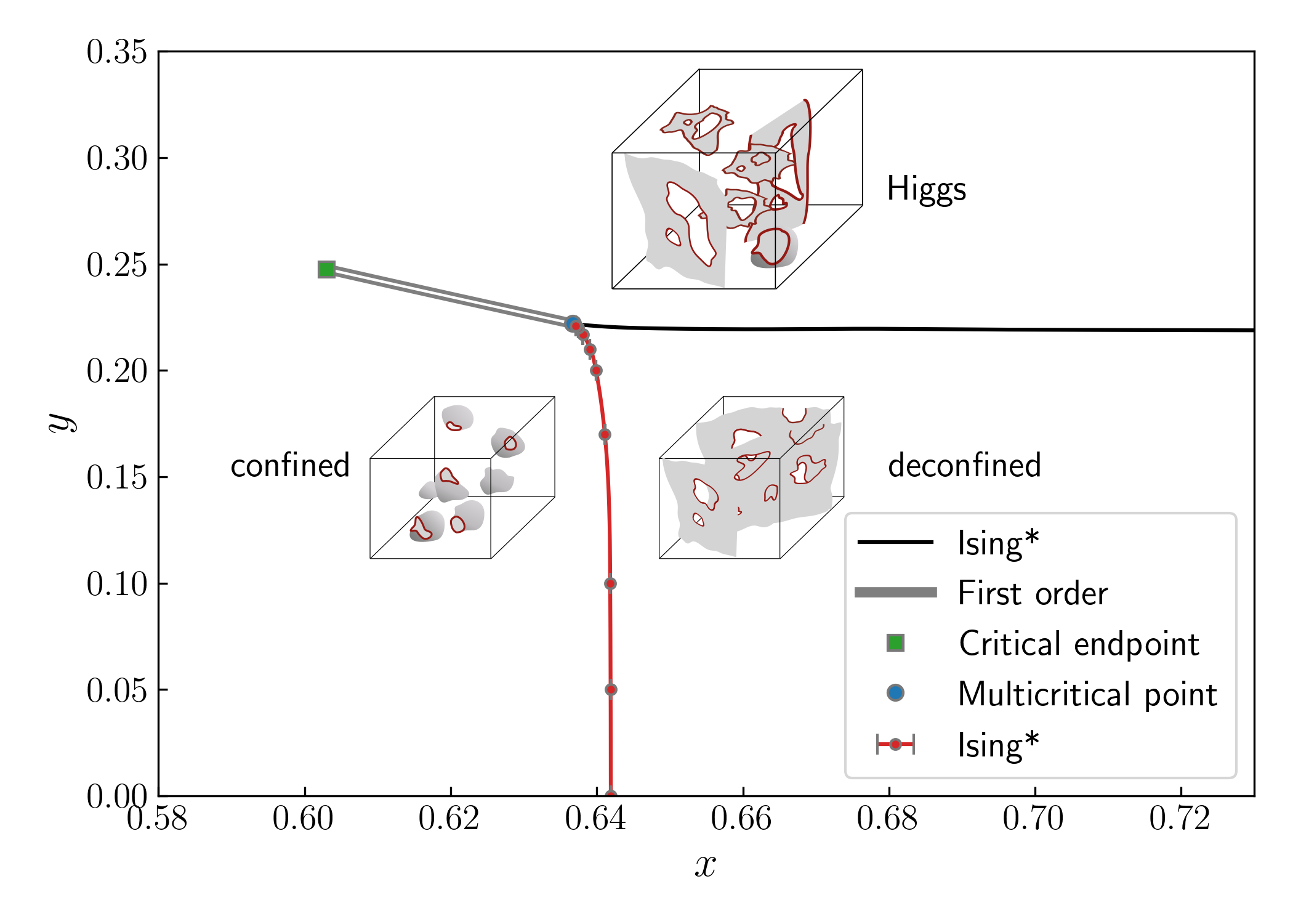
Figure 1: Phase diagram of the $\mathbb{Z}_{2}$ gauge–Higgs model in 3D, showing the confinement transition line (red), the Higgs transition line (black), the self-dual multicritical point (MCP) where they meet, and a segment of first order coexistence extending from the MCP (double line).

When all membranes are closed, the mapping between the gauge theory and a Landau theory (here Ising) is almost trivial. The membranes are simply reinterpreted as domain walls in an Ising order parameter. In this mapping there is a global $\mathbb{Z}_{2}$ ambiguity in the sign of the Ising order parameter, but no additional local ambiguity. When membranes are closed the relevant one-form symmetry is also present microscopically, as we discuss in Sec. II below.

When membranes have holes in them, these mappings break down at the microscopic level. But it is natural to expect that if the holes are “small”, then in the infrared we will effectively recover a theory of closed membranes, in which the above mappings again apply. Here we translate this heuristic point into a constructive approach. The key point is that, whenever the typical size of holes is finite (which we define precisely in terms of percolation) it is possible to repair the membranes, configuration by configuration, by a “patching” procedure [14]. This patching procedure is quasi-local, i.e. it involves patches of finite typical size $\ell$. Crucially, this means that the patching procedure is unambiguous in the thermodynamic limit. It can also be done efficiently in a Monte Carlo simulation, as described below.

Once the membranes have been patched, we can define the configuration of the fictitious order parameter ${S({\bf r})=\pm 1}$, configuration by configuration (up to a global sign, and taking boundary conditions into account). After patching, we can also define topological string operators without any obstacle. The Ising correlation function “$\left\langle S({\bf r})S({\bf r}^{\prime})\right\rangle$” is really the expectation value of such a string operator. The patching procedure allows this correlator to be given a precise meaning and measured in a simulation (perhaps even in an experiment), which would be impossible working only with microscopic observables.

In the 3D $\mathbb{Z}_{2}$ gauge-Higgs model, the Higgs and confinement lines (shown in Fig. 1) are completely equivalent, by the exact duality property of the model [1]. In our convention, the transition line we discuss is the confinement transition. As can be seen in Fig. 1 we can cross this line at various values of the Higgs coupling, which is related to $y$ in the figure. As we move along the confinement phase transition line by increasing $y$, the typical size $\ell$ of the “holes” in the membrane increases, diverging at $y_{\text{MCP}}$, the self-dual critical point where Higgs and confinement lines meet [14, 20]. We study the confinement (Ising^∗) transition at various values of $y$, up to and including $y_{\text{MCP}}$.

Contents

1. I Introduction
2. II $\mathbb{Z}_{2}$ worldsheets: review
   1. II.1 Definition of the model
   2. II.2 The ${y=0}$ limit: closed membranes
   3. II.3 Finite and infinite holes
3. III Membrane patching
   1. III.1 Schematic
   2. III.2 Membrane-patching algorithm
   3. III.3 Ising observables
   4. III.4 Diagnosing the deconfined phase
   5. III.5 Monte Carlo updates
4. IV Application to Ising^∗ transition
   1. IV.1 Dual Ising correlators
   2. IV.2 Other sectors
   3. IV.3 Properties of the patching for large $\ell$
5. V Quasilocality of observables
   1. V.1 Case where $\ell$ is finite
   2. V.2 The self-dual MCP
6. VI Extensions of the patching idea
   1. VI.1 Three dimensions: gauge theories and amphiphilic membranes
   2. VI.2 3+1 dimensions
   3. VI.3 Repairing loops
   4. VI.4 Application to experiments in quantum devices
7. VII Outlook
8. A Scaling arguments
   1. A.1 Lengthscales close to the self-dual MCP
   2. A.2 Fractal structure of patches
   3. A.3 Note on locality of $\widetilde{V}_{P}$

II $\mathbb{Z}_{2}$ worldsheets: review

We will demonstrate the patching procedure for “$\mathbb{Z}_{2}$ membranes” — worldsurfaces of $\mathbb{Z}_{2}$ flux lines in 2+1D. We take the $\mathbb{Z}_{2}$ gauge field to be coupled to a $\mathbb{Z}_{2}$ matter field. We start by reviewing this model. We will be quite brief. See the early parts of Ref. [14] for a more complete overview of the model.

II.1 Definition of the model

The partition function, for an ${L\times L\times L}$ cubic lattice with periodic boundary conditions, is

$$Z\propto\sum_{\{\sigma\},\{\tau\}}\exp\left[K\sum_{\square}\left(\prod_{\left\langle ij\right\rangle\in\square}\sigma_{ij}\right)+J\sum_{\left\langle ij\right\rangle}\tau_{i}\sigma_{ij}\,\tau_{j}\right],$$ (1)

where $i$ labels lattice sites, $\sigma_{ij}=\pm 1$ is the gauge field on links, and $\tau_{i}=\pm 1$ is the Higgs field on sites. We refer to $K$ as the gauge stiffness and to $J$ as the Higgs coupling. However it will be convenient to trade them for the parameterization [1, 29]

$$x =\tanh K, y =\tanh J$$ (2)

(used in Fig. 1), which are the natural “fugacities” in a membrane representation of the partition function [20].

There are two dual ways to formulate the membrane mapping. The equivalence of these dual representations is one way to see the equivalence of the Higgs and confinement phase transition lines in (Fig. 1). In a quantum language, these dual formulations correspond to formulations of the path integral either in the “electric” or the “magnetic” basis, as discussed below. We choose the “electric” representation, in which the membrane ensemble is

$$Z=\sum_{\mathcal{M}}\,x^{|\mathcal{M}|}\,y^{|\partial\mathcal{M}|}.$$ (3)

Here $\mathcal{M}$ stands for a configuration of membranes, which means a set of plaquettes of the cubic lattice that are to be regarded as occupied. See [14] for details. $|\mathcal{M}|$ is the total membrane area of $\mathcal{M}$. The membrane boundary $\partial\mathcal{M}$ is a set of occupied links: A link is part of the membrane boundary $\partial\mathcal{M}$ if it is adjacent to an odd number of occupied plaquettes. $|\partial\mathcal{M}|$ is the total length of occupied links. The left part of Fig. 2 shows an example of a small piece of membrane with a nontrivial boundary.

We will define the term “hole” to mean a geometrically connected subset of $\partial\mathcal{M}$, i.e. a cluster of boundary links (see Sec. III.2 for a more precise definition). It is often useful to idealize holes as loop-like, as explained below (Sec. IV.3), though microscopically they can have more complicated topology.

(Although for convenience we use the word “hole” to denote any connected component of the membrane boundary $\partial\mathcal{M}$, such a boundary component does not need to resemble a hole in a larger piece of membrane: for example, a “hole” could also be the boundary of a small membrane “platelet” made up of a single plaquette.)

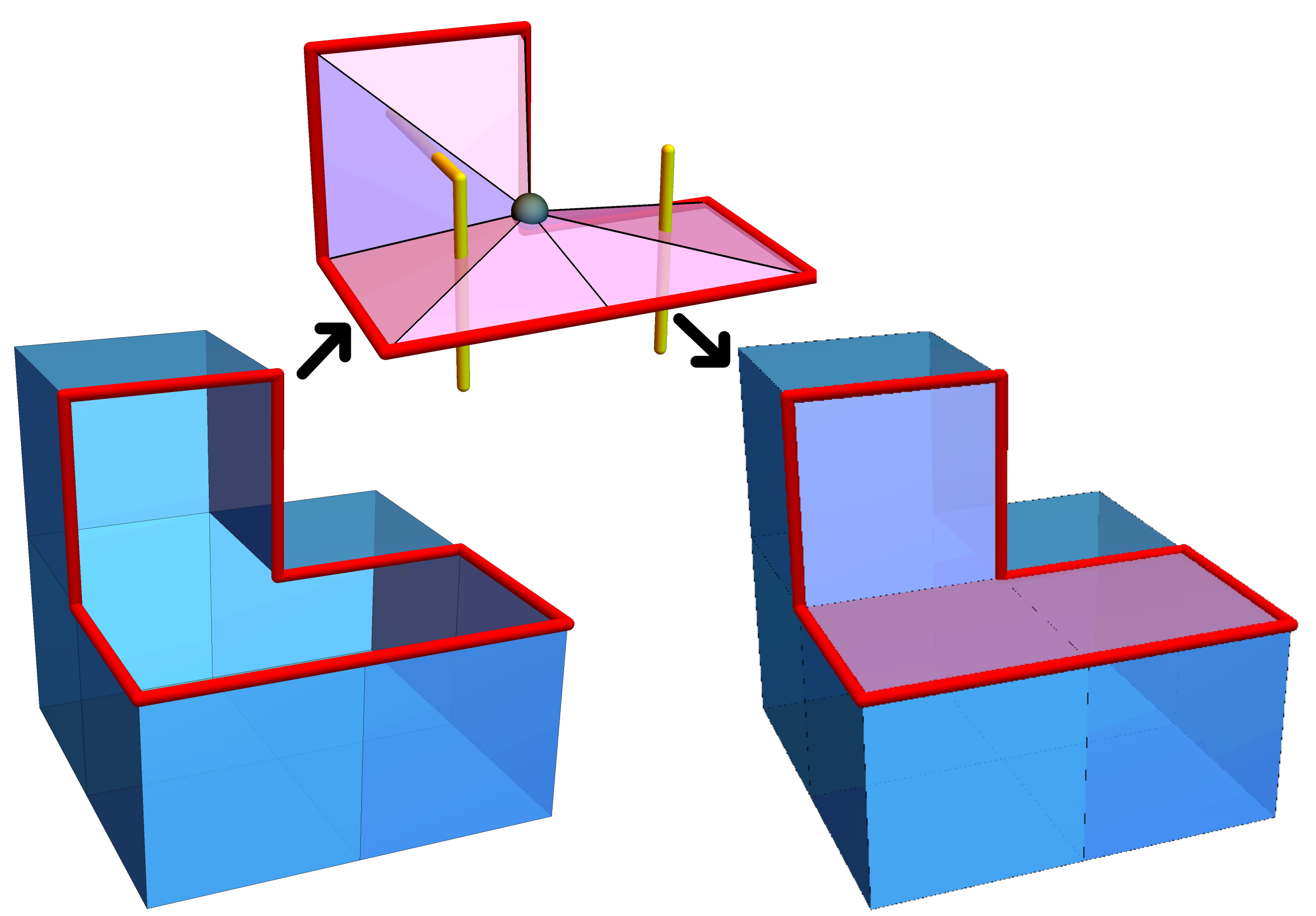
Figure 2: Configuration with a hole and patching scheme (Sec. III.2).

From Eq. 3 we see that $x$ controls the bare membrane tension, and $y$ controls the bare line tension for holes, i.e. for membrane boundary.

Eqs. 1 and 3 can be thought of as 3D classical partition functions in their own right. However, if we choose to think of $Z$ as an imaginary time path integral for a 2+1D quantum $\mathbb{Z}_{2}$ gauge theory, then the membrane ensemble (3) is the formulation of this path integral in the basis of $\mathbb{Z}_{2}$ electric flux lines which live in the 2D spatial plane and which terminate on electric charges. The membranes we are discussing are worldsurfaces of these electric flux lines (see e.g. Fig. 6 in Ref. [14]). The boundaries of the membranes, which make up the “holes”, are worldlines of the electric charges. Duality is the existence of a completely equivalent picture in the magnetic basis, for $\mathbb{Z}_{2}$ magnetic flux lines and charges.

Fig. 1 above showed the phase diagram. The key features are the confinement and Higgs transition lines (related by duality); the self-dual multicritical point at ${(x_{\text{MCP}},y_{\text{MCP}})}$, where confinement and Higgs lines both end [2, 26, 25, 14]; and a short first-order segment to the left of the multicritical point.

We will focus particularly on the confinement transition line, marked in solid red in Fig. 1. If we move along a horizontal line on the phase diagram at fixed $y$ in the range ${[0,y_{\text{MCP}})}$, then we cross this line at an $x$-value that we will denote $x_{c}(y)$. Loosely speaking, crossing this line from the left to the right gives a proliferation of membranes [20].

A key point will be that if we move upwards along a vertical line in the phase diagram, at any fixed $x$, there is a critical value of $y$ where the characteristic size $\ell$ of holes diverges [20, 14]. We will refer to this as the “hole percolation” threshold. The location of the transition line is shown in Fig. 3 below. This threshold coincides with the Higgs transition for ${x>x_{\text{MCP}}}$, and passes through the multicritical point [14]. The percolation transition line also continues to ${x<x_{\text{MCP}}}$, but its nature changes in this regime and it need no longer have any thermodynamic significance for ${x<x_{\text{MCP}}}$.

II.2 The ${y=0}$ limit: closed membranes

The lower boundary of the phase diagram, i.e. the line $y=0$, is special: the partition function simplifies there because the membranes are closed ($\partial\mathcal{M}=0$).

This means that on the line $y=0$ there is a microscopic mapping to Ising [1], and that topological line operators (t’Hooft loops) can be defined microscopically [1, 2, 9, 10, 11, 19]. We now review how this works for $y=0$, in preparation for our main aim which is to extend these mappings and definitions to ${y>0}$.

The closed membranes at $y=0$ can be mapped to Ising domain walls, by introducing Ising spins $S_{r}$ that live at the centres of cubes. (That is, $r$ is a site of the dual cubic lattice, made up of cube centres. A pair of adjacent spins $S_{r}$, $S_{r^{\prime}}$ are antiparallel if the corresponding plaquette $p$ of the original lattice is occupied, i.e. $p\in\mathcal{M}$.) The Ising spin $S$ is ordered for ${x<x_{c}{(0)}}$, i.e. in the confined phase, and $S$ is disordered for ${x>x_{c}{(0)}}$, i.e. in the deconfined phase, where membranes proliferate.

In the finite system, the mapping is to an Ising model with a sum over both periodic and antiperiodic boundary conditions in each direction: this is because a closed path that loops around the system in, say, the $x$ direction can cross either an even or an odd number of membranes. Denoting these two possibilities by ${\sigma_{x}=\pm}$ and similarly for the $y$ and $z$ directions, the gauge theory partition function decomposes into sectors:

$$Z=\sum_{\sigma_{x},\sigma_{y},\sigma_{z}=\pm}Z_{\sigma_{x},\sigma_{y},\sigma_{z}}.$$ (4)

Finally, the relation to the Ising partition function involves a factor of 2, because the above definition of the Ising spin $S_{r}$ has a global sign ambiguity: ${Z_{\sigma_{x},\sigma_{y},\sigma_{z}}^{\text{Ising}}=2Z_{\sigma_{x},\sigma_{y},\sigma_{z}}}$, where on the LHS $\sigma_{\mu}=\pm$ denotes periodic/antiperiodic Ising BCs in the $\mu$ direction.

While there is a “duality” between the gauge theory at ${y=0}$ and the Ising model, the Ising spin $S_{r}$ does not exist as an observable in the original gauge theory. However the gauge theory does have well-defined string operators $V_{P}$ (observables defined on a line) that are closely related to correlators such as ${\left\langle S_{r}S_{r^{\prime}}\right\rangle}$.

Given a path $P$ on the dual lattice (either closed or open), $V_{P}$ is equal to ${+1}$ if $P$ intersects an even number of occupied plaquettes and to ${-1}$ if $P$ intersects an odd number of occupied plaquettes. (We can write $V_{P}$ as a product of local signs for each plaquette pierced by $P$.) Because all membranes are closed when $y=0$, the value of $V_{P}$ does not change if we deform the path $P$ (keeping its endpoints, if any, fixed).

If $P$ is an open path between $r$ and $r^{\prime}$, in an infinite system, then $V_{P}$ depends only on its endpoints. From the domain wall interpretation, it is clear that under the mapping to Ising

$$V_{P}\longleftrightarrow S_{r}S_{r^{\prime}}.$$ (5)

In the finite system with periodic boundary conditions $V_{P}$ is also nontrivial for closed loops that wrap around the system. ($V_{P}$ is trivial for a contractible loop.)

The operators $V_{P}$ can be viewed as symmetry operators [9, 10, 11]. For example, in the Hamiltonian formulation of the gauge theory, as a 2D quantum system, one may define corresponding unitary quantum operators $\hat{V}_{P}$ for paths $P$ lying in the spatial plane. The invariance of $V_{P}$ under deformations of $P$ implies that these operators commute with the Hamiltonian: ${[\hat{H},\hat{V}_{P}]=0}$. Unlike the generators of a conventional symmetry (which would be supported on the entire spatial plane) these operators are supported on one-dimensional lines. They are referred to as 1-form symmetry operators.

In this language, the one-form symmetry is spontaneously broken in the deconfined phase, because of the existence of a degenerate ground state manifold within which $\hat{V}_{P}$, for winding loops, acts nontrivially. In the language of the $\mathbb{Z}_{2}$ topological order and the toric code, $\hat{V}_{P}$ are the “magnetic” string operators associated with “m” excitations [19].

II.3 Finite and infinite holes

The above concepts (the “dual” Landau order parameter $S_{r}$, and the string operators) are useful for detecting the deconfined phase and the transition out of it. To generalize them to ${y>0}$, we will need to deal with the problem of having holes in the membranes. We make some qualitative points before giving a concrete construction in the next Section. For concreteness we focus the discussion below on the confinement transition, but the key points also apply in the deconfined phase. By duality, the discussion also translates directly to the Higgs transition. We will discuss some other extensions of the method in Sec. VI.

Let ${\ell(y)\equiv\ell\big{(}x_{c}(y),y\big{)}}$ be the typical hole size at a given point along the confinement transition line. $\ell(y)$ grows with increasing $y$, and diverges at the MCP. Fig. 3 shows the part of the phase diagram where $\ell$ is finite.

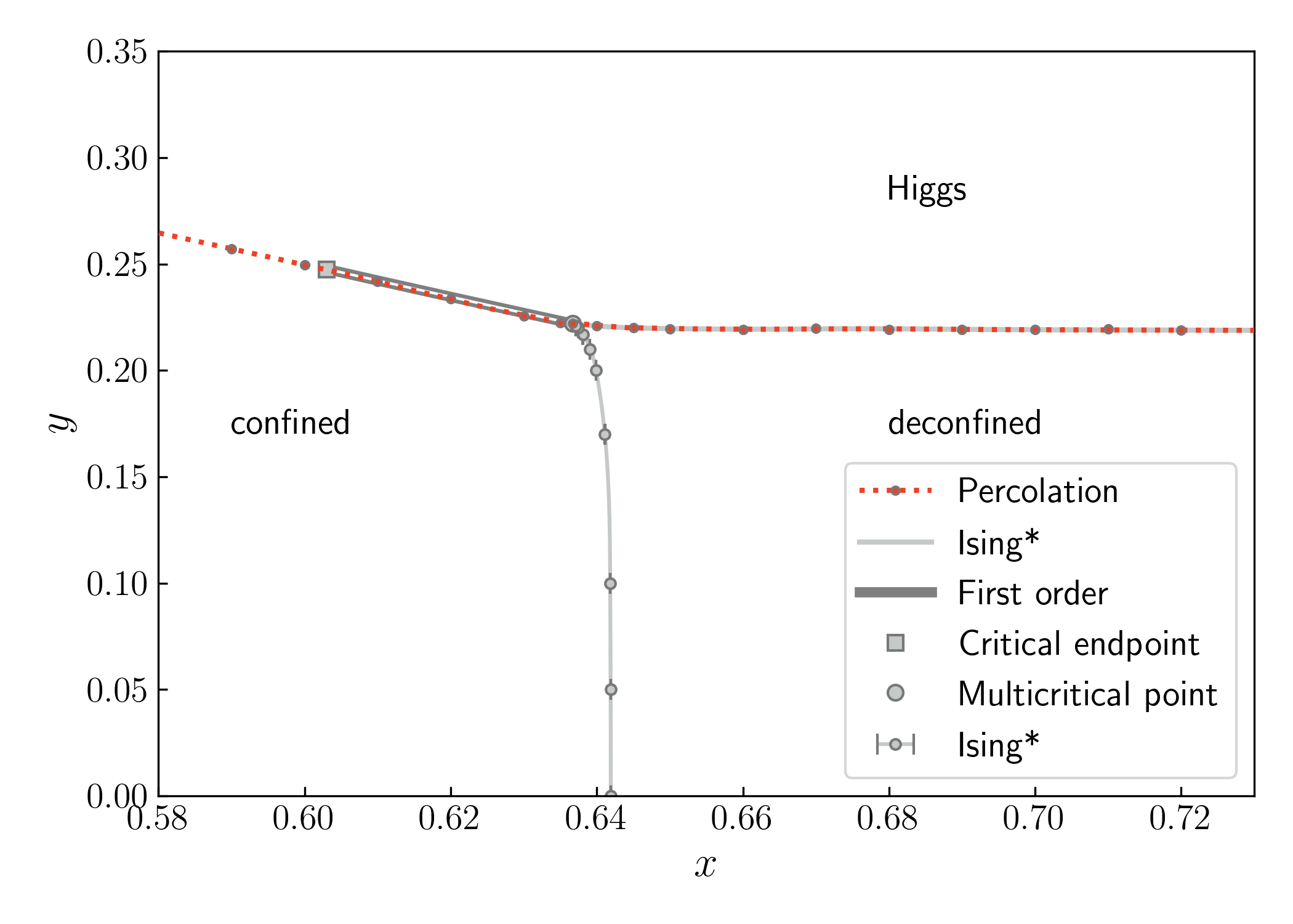
Figure 3: The phase diagram of Fig. 1 shown together with the percolation threshold for holes (red dashed line). The typical hole size $\ell(x,y)$ is finite below this line (data from [14]).

Heuristically, when $\ell(y)$ is finite (${y<y_{\text{MCP}}}$), we might imagine that holes disappear under RG. That is, after coarse-graining to scales ${\gg\ell(y)}$ we effectively recover a theory of closed membranes, and the system flows to the same Ising^∗ fixed point that governs the phase transition on the boundary ${y=0}$. Below we will show that this can be made concrete (giving a constructive mapping to Ising) also for ${y>0}$.

We construct the dual spin $S_{r}$ explicitly and show that it only behaves like a local operator on scales much larger than $\ell(y)$. Therefore the duality to Ising only emerges beyond this scale.

Similarly string operators analogous to $V_{P}$ can be defined as “fattened” objects [13]. Because of rare large loops, the string operators must in general be much thicker than $\ell(y)$, as we discuss below.

We will also examine the fate of these concepts at the multicritical point (MCP), where $\ell=\infty$ and “holes” are present on all scales. We emphasise that the MCP is in a different universality class to the confinement line. Monte Carlo strongly indicates that the multicritical point is a scale-invariant critical point, which is of interest because it is a simple example of a critical point without any known useful continuum Lagrangian description [14].

The dual order parameter $S_{r}$ ceases to be local at the multicritical point (MCP). This is one way of understanding why the mapping to a Landau theory breaks down at the MCP (see Refs. [14, 28] and Sec. VII for further discussion of this point).

Interestingly, though, there is a sense (discussed in Sec. V.2 below) in which this nonlocality is mild at the MCP. This may be a hint as to why various exponents at the multicritical point are numerically close to exponents of the XY model [14, 27].

III Membrane patching

III.1 Schematic

To define the dual order parameter and the string operators, we will define a convention for mapping a given membrane configuration $\mathcal{M}$ — which in general will have a nontrivial boundary, ${\partial\mathcal{M}\neq 0}$ — to a “repaired” or “patched” configuration $\overline{\mathcal{M}}$ with ${\partial\overline{\mathcal{M}}=0}$. Once this is done, $\overline{\mathcal{M}}$ can be viewed as a configuration of domain walls for a dual spin $S_{r}$, and observables can be constructed in terms of $\overline{\mathcal{M}}$ in the same way as at ${y=0}$.

We emphasize that this is a procedure for defining observables in a given configuration $\mathcal{M}$ — we leave the partition function unchanged. In particular, above we defined string operators $V_{P}(\mathcal{M})$ in the closed membrane ensemble (here we have made the dependence of this observable on the configuration $\mathcal{M}$, as well as on a path $P$, explicit). The patching procedure allows us to define a string operator $\widetilde{V}_{P}$ in the ${y>0}$ ensemble, via:

$${\widetilde{V}_{P}(\mathcal{M})\equiv V_{P}(\overline{\mathcal{M}})}.$$ (6)

Since $\overline{\mathcal{M}}$ is closed, $\widetilde{V}_{P}$ has the key invariance property under deformations of the path $P$. For an open path $P$ between points $r$ and $r^{\prime}$ in an infinite system we have the duality relation ${\widetilde{V}_{P}(\mathcal{M})\leftrightarrow S_{r}S_{r^{\prime}}}$ (we discuss boundary conditions in a finite system below).

We will perform the repair by attaching a patch for each hole separately (by the rule in the following subsection). Note that the mapping from $\mathcal{M}$ to $\overline{\mathcal{M}}$ is not a strictly local operation: a given plaquette in $\overline{\mathcal{M}}$ depends on other plaquettes in $\mathcal{M}$. In turn, this relaxes the locality properties of $\widetilde{V}_{P}$ and the dual spin $S_{r}$. However, if the typical hole size is finite, there is an effective notion of locality on larger scales [14], which we discuss in Sec. V.

We now describe concretely how to define the patching. In following sections we will implement it in a Monte Carlo simulation of Eq. 3, focussing particularly on the confinement transition for ${0<y<y_{MCP}}$.

III.2 Membrane-patching algorithm

The membrane-patching algorithm is as follows. For a given configuration $\mathcal{M}$, the first step consists in performing a percolation analysis of the occupied links (links in ${\partial\mathcal{M}}$). This means that we determine the connected clusters of links. (A cluster does not share any site with any other cluster.)

If there is a cluster that spans the entire system in any direction then we flag the configuration as percolating (“non-patchable”), and do not try to patch it. Later when we compute expectation values, we will often condition on the configuration being patchable (non-percolating). When ${y<y_{\text{MCP}}}$, the probability of a configuration percolating is vanishingly small at large $L$.

In a given patchable configuration, we patch each cluster separately. The links of a cluster represent the boundary of a patching surface: see for example the left image in Fig. 2. It is convenient to think of the definition of this surface as a two-step procedure.

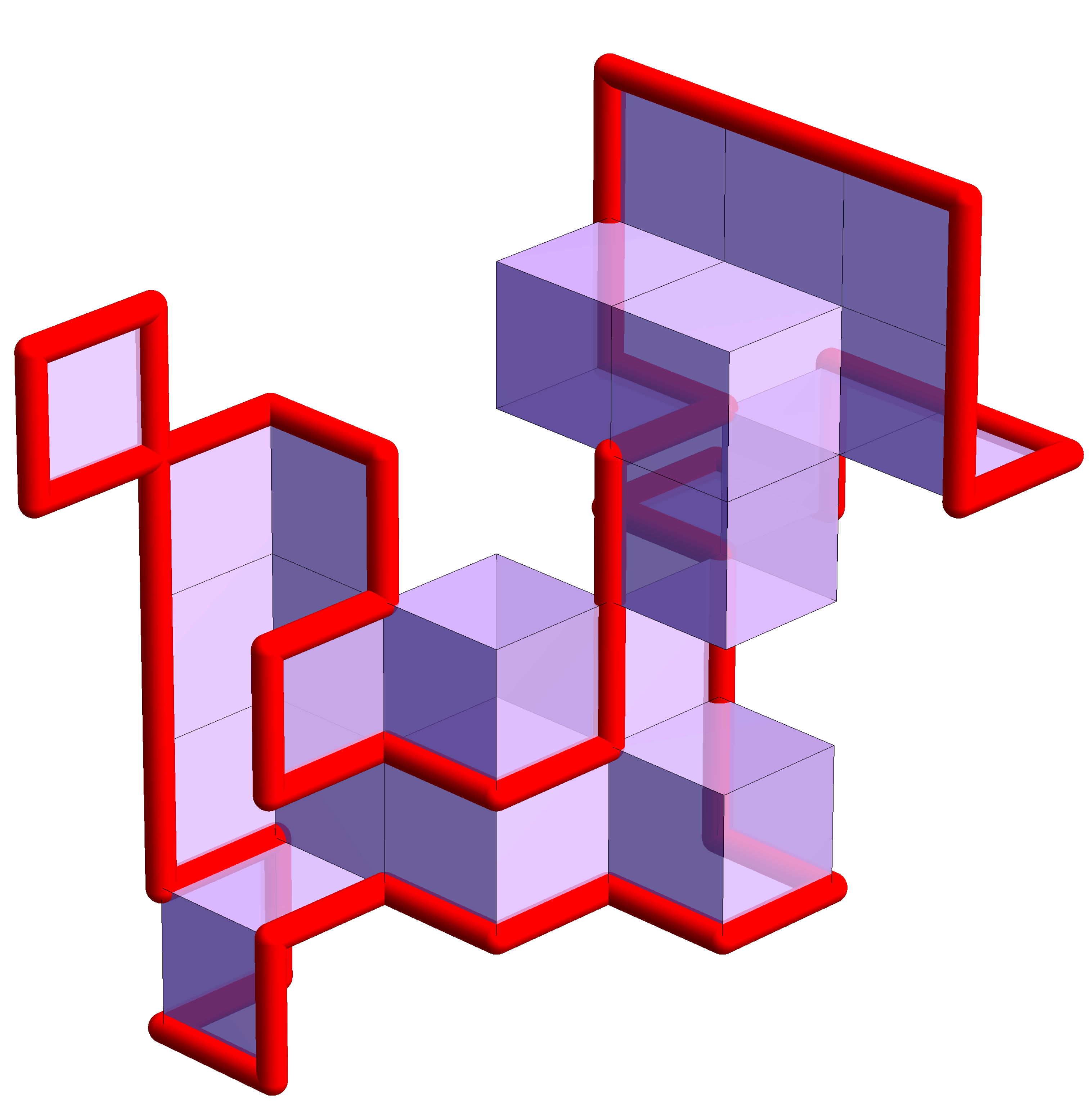
Figure 4: A loop configuration (“hole”) and the resulting membrane patch produced by the algorithm.

First, a patching surface can easily be constructed as a union of triangles. For each link in the cluster, we define a triangle with the link as one side and the cluster’s center of mass as the opposite vertex. Such a surface is shown in the central image in Fig. 2.

Next, we simplify this surface to an equivalent one constructed from plaquettes of the cubic lattice, instead of from triangles (Fig. 2, Right). Note that each plaquette $p$ is dual to a link $l(p)$ of the dual cubic lattice (lines in yellow in the central image in Fig. 2). Loosely speaking, if a triangle crosses a dual link $l(p)$, this means that the plaquette $p$ should be included in the patch. More precisely, a plaquette $p$ is included if the dual link $l(p)$ crosses an odd number of triangles. An example of the membrane patch associated to a cluster is shown in Fig. 4.

A final detail is that in rare cases a triangle may pass exactly through a vertex of the dual cubic lattice. For a simple solution, we resolve the degeneracy by infinitesimally perturbing the centre of mass in a random direction. Other resolutions are possible, but the choice will not have any significant effect on the results.

Having defined the patches we can define the repaired configuration $\overline{\mathcal{M}}$. If we call the set of patching plaquettes ${\cal P}$, the new set $\overline{\mathcal{M}}={\cal M}\cup{\cal P}-{\cal M}\cap{\cal P}$ defines strictly closed surfaces and allows us to construct line operators as described in Sec. III.1.

III.3 Ising observables

In particular, we can define correlators of the dual Ising field, e.g. ${\left\langle S_{r}S_{r^{\prime}}\right\rangle}$, if we correctly account for boundary conditions (as discussed directly below). We propose that these correlators are practically useful for the analysis of the phase transition, because they allow standard tools for order parameters to be applied to the confinement and Higgs transitions, despite the fact that the original model does not have an order parameter. For example, such tools include the analysis of the total magnetization, and of Binder cumulants, to accurately identify the transition point. (We will use the language of the confinement transition, but by duality, the results translate directly to the Higgs transition.) We reiterate that for $y>0$ the quantity $S_{r}S_{r^{\prime}}$ is definable only through the patching procedure, unlike the simpler case $y=0$ where $S_{r}S_{r^{\prime}}$ is the expectation value of a “microscopic” line operator.

As discussed around Eq. 4, an ensemble of closed membranes can be split into sectors. Our patching algorithm works in all sectors, but for some observables we will restrict to the first sector (${\sigma_{x}=\sigma_{y}=\sigma_{z}=+}$). In this sector the dual Ising spin $S_{r}$ has periodic boundary conditions and so is well-defined up to a global sign flip, so that after patching the correlation function $\left\langle S_{r}S_{r^{\prime}}\right\rangle$ may be straightforwardly defined. When we write expressions such as $\left\langle S_{r}S_{r^{\prime}}\right\rangle$, we refer to an average conditioned on the ${\sigma_{x}=\sigma_{y}=\sigma_{z}=+}$ sector.

(More formally, this may be expressed as

$$\left\langle S_{r}S_{r^{\prime}}\right\rangle\equiv\frac{\left\langle\widetilde{V}_{P}(\mathcal{M})\,\chi_{+}(\mathcal{M})\right\rangle}{\left\langle\chi_{+}(\mathcal{M})\right\rangle},$$ (7)

where $P$ is any path connecting $r$ to $r^{\prime}$, and $\chi_{+}(\mathcal{M})$ is an indicator function that takes the value $\chi_{+}=1$ if $\mathcal{M}$ is a patchable configuration in the $+++$ sector, and the value $\chi_{+}=0$ otherwise.)

Similarly, for a configuration in the ${\sigma_{x}=\sigma_{y}=\sigma_{z}=+}$ sector, the squared magnetization density

$$M^{2}=\Big{(}L^{-3}\,{\sum}_{r}S_{r}\Big{)}^{2}$$ (8)

is well-defined.

In the simulations below it will also be convenient to define two dimensionless quantities:

$$\operatorname{b}_{4}(M) =\frac{3\left\langle M^{2}\right\rangle^{2}-\left\langle M^{4}\right\rangle}{2\left\langle M^{2}\right\rangle^{2}},$$ (9)

$$\operatorname{b}_{1}(M) =\frac{1}{1-\sqrt{2/\pi}}\left(\frac{\left\langle|M|\right\rangle}{\left\langle M^{2}\right\rangle^{1/2}}-\sqrt{\frac{2}{\pi}}\,\right).$$ (10)

$\operatorname{b}_{4}(M)$ is just the Binder parameter [30] rescaled such that it becomes 1 in the ferromagnetic phase and 0 in the paramagnetic one ($\operatorname{b}_{4}=3U_{L}/2$). $\operatorname{b}_{1}(M)$ behaves similarly to $\operatorname{b}_{4}(M)$ and has the same two limits, but it is statistically slightly easier to estimate [14], so we suggest the use of the former instead of the latter.

We will also store statistics related to the total patched area, which we denote $A_{\text{patched}}$: for a given configuration, $A_{\text{patched}}$ is the number of plaquettes in the set $\mathcal{P}$ defined above in Sec. III.2. Analysis of the statistics of $A_{\text{patched}}$ at different points on the confinement line reveals the divergence of the patching lengthscale $\ell(y)$ as the self-dual critical point is approached.

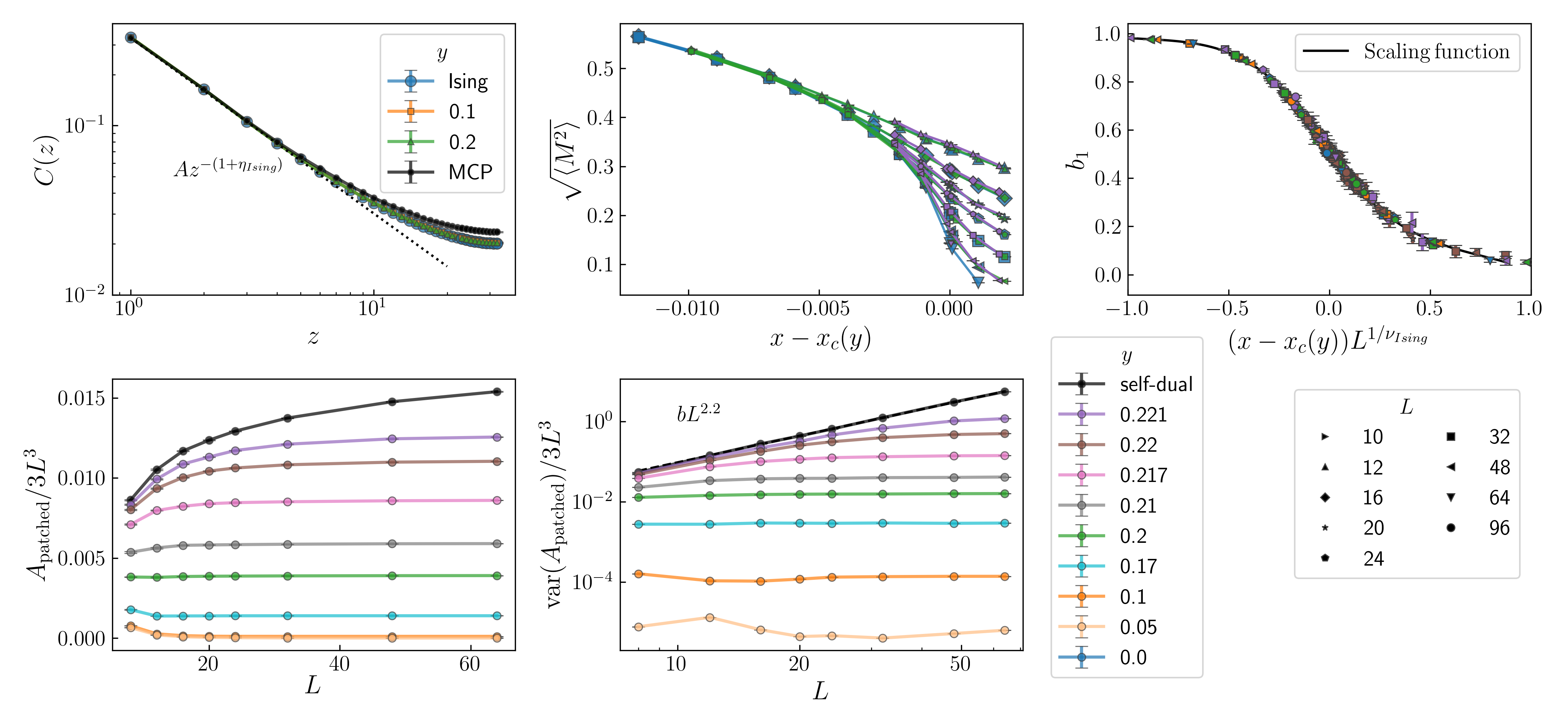
Figure 5: Panel 1 – Correlation as a function of distance along one of the axis directions for system size $L=64$ at the critical point $x_{c}(y)$ for several values of $y$. Black dotted line represents a power-law $r^{-(1+\eta_{\mathrm{Ising}})}$, where $\eta_{Ising}=0.036298$. Panel 2 – Magnetization as a function of ${x-x_{c}(y)}$, for several values of $y$ and different system sizes. Colours and symbols indicate $y$ values (three are plotted) and system sizes, respectively. Panel 3 – Scaling collapse of parameter $b_{1}$ as a function of ${(x-x_{c}(y))L^{1/\nu_{\mathrm{Ising}}}}$ where $\nu_{\mathrm{Ising}}=0.629971$ is the critical exponent of the 3D Ising universality class. Panel 4 – Patched area for several values of $y$ as a function of $L$ at their critical point $x_{c}(y)$. Panel 5 – Variance of the patched area for several values of $y$ as a function of $L$ in logarithmic scale, at their critical point $x_{c}(y)$.

III.4 Diagnosing the deconfined phase

Since in Sec. IV we will focus on critical scaling near the confinement transition line, we emphasize here that the patching procedure gives a way to characterize the deconfined phase more generally (i.e. even far from the confinement transition line). The deconfined phase is the part of the phase diagram where both ($i$) and ($ii$) hold:

($i$) The patching procedure succeeds: i.e. the probability of a configuration $\mathcal{M}$ being patchable tends to 1 at large system size. Equivalently, the holes are non-percolating.

($ii$) The dual Ising order parameter is disordered, as manifested, for example, in the vanishing of $\left\langle M^{2}\right\rangle$ at large $L$. Equivalently, the expectation value of the string operator ${\lim_{L\to\infty}\langle\widetilde{V}_{P}\rangle}$, for an open path of length $R$, tends to zero at large $R$.

III.5 Monte Carlo updates

For completeness we specify the updates used to equilibrate the model. For one Monte Carlo step we use two standard Metropolis updates: First we attempt to update all plaquettes in the system (one at at a time). Second, for all cubes in the system, we try to change all six plaquettes of the cube at the same time. For ${y=0}$ this second procedure reproduces the standard spin-flip update for the dual Ising system.

IV Application to Ising^∗ transition

We now apply the above algorithm to the confinement phase transition (${y<y_{\text{MCP}}}$). By the exact self-duality of the gauge theory, the following results also apply to the Higgs transition, in the dual membrane representation (where the membranes are worldsheets of magnetic, rather than electric, fluxlines).

First we show results for dual Ising observables which are computable using this patching algorithm. Then we study the properties of the patches themselves: these reveal a growing lengthscale $\ell(y)$, and a fractal structure below this scale, when $y$ gets close to $y_{\text{MCP}}$.

IV.1 Dual Ising correlators

We study the phase transition at several values of $y$. For a given value of $y$, the critical value $x_{c}(y)$ can be determined using the modified Binder cumulant $b_{1}$ (Eq. 10), which shows a crossing at $x_{c}(y)$, and is discussed further below.

A striking demonstration of Ising^∗ universality is given by the power-law scaling of the dual Ising correlator as a function of separation $z$:

$$C(z)=\langle S_{(0,0,0)}S_{(0,0,z)}\rangle$$ (11)

at the critical point ${x=x_{c}(y)}$. At $y=0$ this correlator can be defined microscopically using a simple line operator, but for $y>0$ it is nontrivial and must be defined using the patching procedure.

The correlator is shown in Panel 1 of Fig. 5, as a function of distance $z$ in a system of fixed size $L=64$. Data for the values ${y=0,0.1,0.2}$, which lie on the confinement line and are expected to be in the Ising^∗ universality class, are consistent with the Ising power law, where $\eta_{\mathrm{Ising}}=0.036298(2)$ [31], which is shown with a dotted line. (Since the Ising anomalous dimension $\eta_{\text{Ising}}$ is small, this line is close to $1/z$.) The distinct curves are also consistent with each other within error bars: although in general the nonuniversal normalization of $C(z)$ will depend on $y$, this dependence appears to be very weak. The Panel also shows the correlator computed at the MCP, where its RG interpretation is different and will be discussed in Sec. V.2.

An intuitive way to see the confinement transition is in the dual magnetization (Eq. 8), shown as a function of ${x-x_{c}(y)}$ in Panel 2 of Fig. 5. Data is shown for different systems sizes and also different $y$. Again, $y=0$ is the case where there is a microscopic mapping to Ising. This is compared with the same quantity for ${y=0.2}$ and ${y=0.221}$. They both show a striking similarity to the ${y=0}$ case. Note that we have absorbed the $y$-dependent shift to the location of the critical point (which can be seen in Fig. 1) so that the transition occurs at the same value of the horizontal coordinate in each case.

Finally, Panel 3 of Fig. 5 shows the scaling collapse of $b_{1}$ for several values of $y<y_{MCP}$ using the known Ising correlation length exponent $\nu_{\mathrm{Ising}}=0.629971(4)$ [31]. We fitted all data to a single scaling function, shown in the figure as a black line. For the scaling function we used 8 free paramaters (8 coefficients for a B-spline function). Additionally, in order to achieve collapse of the curves we kept $x_{c}(y)$ as an adjustable parameter for each y value used.

Using data for $y\leq 0.217$ and dropping the smaller system sizes we obtained $\chi^{2}=42.04$ for 39 degrees of freedom, showing an excellent overlap between different locations on the phase transition line. We also obtained accurate phase boundaries $x_{c}(y)$ from the fit. These agree within error bars with the estimates using percolation observables in [14] (the latter estimated the Higgs phase boundary, but duality relates it to the confinement boundary under discussion here). In the panel we also show data for smaller sizes, as well as data for $y=0.22,0.221$ that were not used for fitting, and the deviation from the scaling curve is still quite small.

IV.2 Other sectors

The observables above are expectation values conditioned on being in the first sector (${\sigma_{x}=\sigma_{y}=\sigma_{z}=+}$) of the membrane ensemble. It is of course possible to consider observables averaged over sectors.

A simple one is the probability $P_{\sigma_{x},\sigma_{y},\sigma_{z}}$ of being in a given sector. Note that the value of $\sigma_{x}=\pm 1$ is just the value of the string operator $\widetilde{V}_{P_{x}}$ for a path $P_{x}$ that winds around the sample in the $x$-direction, so $P_{\sigma_{x},\sigma_{y},\sigma_{z}}$ is simply related to expectation values of such winding string operators.

At the Ising^∗ critical point, and in the limit $L\rightarrow\infty$, these numbers are universal and related by duality to ratios of Ising partition functions with different boundary conditions,

$$P_{\sigma_{x},\sigma_{y},\sigma_{z}}=\frac{Z^{\text{Ising}}_{\sigma_{x},\sigma_{y},\sigma_{z}}}{\sum_{\sigma_{x}^{\prime},\sigma_{y}^{\prime},\sigma_{z}^{\prime}}Z^{\text{Ising}}_{\sigma_{x}^{\prime},\sigma_{y}^{\prime},\sigma_{z}^{\prime}}}.$$ (12)

In a finite-size system, there is also a nonzero probability $P_{\text{perc}}(L)$ of being in a percolating (non-patchable) configuration, which is not assigned to any of the above sectors. For ${y<y_{\text{MCP}}}$ this probability vanishes exponentially at large $L$, so that (asymptotically) every configuration can be assigned to an Ising sector.

For ${y=y_{\text{MCP}}}$, where ${\ell=\infty}$, the limit $\lim_{L\rightarrow\infty}P_{\text{perc}}(L)$ is instead a nonzero constant, which we estimate in Sec. V.2 (Table 1).

In our Monte Carlo dynamics, the configuration can make a transition between different sectors by passing through a non-patchable configuration with a percolating hole. In principle this allows equilibration over all sectors. In practice this is possible if $y$ is not too small and $L$ is not too large. When $y<y_{\text{MCP}}$ such transitions are exponentially suppressed in the limit $L\rightarrow\infty$ simply because $P_{\text{perc}}(L)$ is exponentially suppressed. For this reason we have not tried to accurately compute the sector probabilities for the Ising^∗ critical point. This could be done, using the present gauge theory, by parallel tempering, exchanging configurations at different values of $y$ [32].

IV.3 Properties of the patching for large $\ell$

As $y$ increases along the confinement line, approaching the multicritical point at $y_{\text{MCP}}$, the “holes” in the membranes become larger. Structurally, these holes are clusters of links on the cubic lattice. At the MCP, and on scales much larger than the lattice spacing, they become fractal loops with a fractal dimension [14]

$$d_{f}=1.77(2)$$ (13)

Slightly below $y_{\text{MCP}}$, the typical size $\ell(y)$ of the holes is finite (a discussion of scaling forms close to the MCP is given in App. A):

$$\ell(y) \sim\frac{1}{(y_{\text{MCP}}-y)^{\nu_{S}}}, \nu_{S} \simeq 0.67,$$ (14)

where ${\nu_{S}=(3-x_{S})^{-1}}$ is a critical exponent of the MCP [14]. The loops are fractals on scales in between 1 and $\ell(y)$.

Once the holes are patched, the patches inherit some fractal properties from their boundaries. For example, the typical area of a large patch scales with its linear size $R$ as $R^{1+d_{f}}$: that is, the effective dimensionality of the patch is greater by one than the effective dimensionality of its boundary, as we might have expected.

Here, we show that the diverging lengthscale $\ell(y)$ has implications for the statistics of the total patched area, $A_{\text{patched}}$, defined at the end of Sec. III.3. We compare simulation data with expectations from a scaling argument in that is described in App. A.

Below we describe the approach to the MCP along the confinement line; qualitatively similar results, but with slightly different exponent values, would obtain if we approached the Higgs phase transition from within the deconfined phase, since $\ell$ also diverges on the Higgs line.

In Panel 4 of Fig. 5, the average fraction of plaquettes that get patched — i.e. $\left\langle A_{\text{patched}}\right\rangle/3L^{3}$, where $3L^{3}$ is the total number of plaquettes in the lattice – is shown as a function of the system size, for several values of $y$. The fraction of patched plaquettes increases slowly as $y\rightarrow y_{\text{MCP}}$, indicating that the typical density and/or size of the holes is growing. However ${\lim_{L\rightarrow\infty}\left\langle A_{\text{patched}}\right\rangle/3L^{3}}$ is finite even at the MCP (as it must be since by definition this fraction is between zero and one). At the MCP we may argue

$$\frac{\left\langle A_{\mathrm{patched}}(L)\right\rangle}{3L^{3}}=\alpha-{\beta}{L^{-(2-d_{f})}}+\ldots.$$ (15)

where $\alpha$ and $\beta$ are constants. The first term is dominated by small loops, while the exponent in the subleading term is universal. On the confinement line, in the regime ${1\ll\ell(y)\ll L}$, the form is instead

$$\frac{\left\langle A_{\mathrm{patched}}(L)\right\rangle}{3L^{3}}=\alpha-\gamma(y_{\text{MCP}}-y)^{\nu_{S}(2-d_{f})}+\ldots,$$ (16)

where this exponent is $\sim 0.15$ (this is consistent with extrapolated data from Panel 4 Fig. 5 – data not shown).

Unlike the above average, higher moments of $A_{\text{patched}}$ are dominated by the largest patches, and do show a critical divergence arising from the divergence of the typical patch size $\ell$.

When $\ell$ is finite, the normalized cumulants $\langle\langle A^{k}\rangle\rangle/(3L^{3})$ for ${k=2,3,\ldots}$ have a finite thermodynamic limit, but at the MCP we expect that they are dominated by patches with linear size comparable with $L$, so scale as $\langle\langle A^{k}\rangle\rangle/(3L^{3})\sim L^{k(1+d_{f})}/L^{3}$. For $y$ close to $y_{\text{MCP}}$,

$$\langle\langle A_{\text{patched}}^{k}\rangle\rangle=L^{k(1+d_{f})}F^{(k)}(L/\ell),$$ (17)

where $\ell$ is the lengthscale in (14) and $F^{(k)}$ is a crossover scaling function.

Panel 5 of Fig. 5 shows the normalized variance of the patched area,

$$\langle\langle A_{\text{patched}}^{2}\rangle\rangle/(3L^{3})$$ (18)

as a function of the system size, for various $y$. For $y<y_{\text{MCP}}$, this quantity has a finite thermodynamic limit. At the MCP, the data is consistent with a power-law divergence in $L$, as $\langle\langle A_{\text{patched}}^{2}\rangle\rangle/(3L^{3})\sim L^{2.2}$. This exponent is smaller than the expected $L^{2.54}$. We have not identified the source of the discrepancy. Conceivably, finite size effects associated with the internal structure of a cluster may be large. We discuss some aspects of cluster structure in App. A.

Nevertheless, the divergence of the variance of the patched area is a clear sign of a diverging lengthscale for patches at the MCP.

V Quasilocality of observables

Here we discuss the locality properties of the line operators $\widetilde{V}_{P}$ defined in Sec. III.1 and of the dual Ising variable. First we discuss the case where the typical loop (hole) size $\ell$ is finite: in this case there is a notion of locality after coarse-graining, confirming that patching successfully defines emergent string operators and the emergent “duality” to a local order parameter. Then in Sec. V.2 we discuss the case where $\ell$ diverges in order to clarify in what sense locality breaks down.

V.1 Case where $\ell$ is finite

Consider the regime where $\ell$ is finite (though perhaps large): this includes the deconfined phase and the confinement critical regime discussed above (and part of the trivial phase). The following points were discussed more briefly in Ref. [14].

How local are the string operators $\widetilde{V}_{P}$? First let us consider a closed path $P$. For concreteness, let $P$ be a straight path of length $L$ (on the dual lattice) that winds around a periodic system of size $L$.

When $\ell=0$, the operators (t’Hooft operators) $V_{P}$ are supported on a single line of plaquettes: i.e. the value of $V_{P}(\mathcal{M})$ is a product of $\pm 1$ factors associated with the plaquettes lying on $P$, and so they can be determined by examining the configuration $\mathcal{M}$ only along this line. For $\ell>0$, the value of ${\widetilde{V}_{P}(\mathcal{M})=\pm 1}$ is defined through patching. In order to determine this value, we must determine which of the plaquettes on $P$ are occupied in the patched configuration $\overline{\mathcal{M}}$.

In principle this can depend on plaquettes of $\mathcal{M}$ that are far from $P$. However, to determine ${\widetilde{V}_{P}(\mathcal{M})=\pm 1}$ with a high probability (say $1-\epsilon$) of success, it is not necessary to patch the entire configuration $\mathcal{M}$. It is sufficient to patch the loops (holes) in a “tube” around $P$. This tube must be large enough to include, with high probability, all the loops that are pierced by $P$.

At first sight we might think that it is sufficient to take a tube of thickness $\mathcal{O}(\ell)$, since this is the typical loop size. However, if the length $L$ of the path is much larger than $\ell$, then the path will likely encounter some “rare” loops of size $\gg\ell$. This requires us to thicken the tube to a radius that is of order

$${R\sim\ell\ln(L/\epsilon)}$$ (19)

when $L$ is large, in order to have a high probability that all the relevant loops are included in the tube. (See App. A.3 for more detail.)

In other words, we can accurately approximate $\widetilde{V}_{P}$ with an operator $\widetilde{V}_{P}^{\epsilon}$ which is a function only of the configuration inside a tube of thickness $R$ around $P$ (and which agrees with $\widetilde{V}_{P}$, in a random configuration $\mathcal{M}$, with a probability very close to 1). Note that $R$ is parametrically smaller than the length of the path $P$, so that after sufficient coarse-graining the (t’Hooft) line operator $\widetilde{V}_{P}$ can be regarded as local.

Now consider an open path $P$. Letting $P$ be a straight path between two points $r$ and $r^{\prime}$, we can approximate $\widetilde{V}_{P}$ by an operator that depends only on the configuration inside a cigar-shaped region surrounding $P$, whose thickness at the centre is of order ${\ell\ln(|r-r^{\prime}|/\epsilon)}$. The thickness of the cigar close to its endpoints, however, can be taken to be only of order $\ell$. In (say) an infinite system, the operator $\widetilde{V}_{P}$, for such an open path $P$, is dual to ${S_{r}S_{r^{\prime}}}$.

The invariance of $\widetilde{V}_{P}$ under deformations of the path $P$ means that ${S_{r}S_{r^{\prime}}}$ can be mapped to $\widetilde{V}_{P}$ for any path $P$ connecting $r$ to $r^{\prime}$. This, together with the observations above about the cigar-shaped region around $P$, gives a sense in which $\ell$ is a typical scale associated with the dual operator $S$. Loosely speaking, a product such as $S_{r}S_{r^{\prime}}$ is robust to changes in the membrane configuration, so long as these changes are far enough away from $r$, $r^{\prime}$ and sufficiently local.

An alternative way to quantify locality in the dual language would be to reexpress the partition function in terms of $S_{r}$. Because of patching the effective interactions would be nonlocal, but could be approximated by interactions of finite range $\mathcal{O}(\ell)$ at the cost of incurring only a small error in the free energy density.

We can also consider the effect on operators $\widetilde{V}_{P}$ of changing the patching scheme. If the new scheme retains similar locality properties to the present one, the change only dresses $\widetilde{V}_{P}$ by quasilocal (on scale $\ell$) functions of the membrane configuration near $P$’s endpoints. This does not affect the universal asymptotics of correlation functions.

The point above about rare worldline configurations (of the gapped anyon), which gave the scaling in Eq. 19, should apply generally to the Euclidean path integrals for topological phases. It indicates that generically their emergent line operators must have a thickness that grows logarithmically with their length. This logarithmic scaling is consistent with bounds for quantum operators in Ref. [13], which considered the definition of dressed line operators, obtained by quasiadiabatic continuation, in discrete gauge theories.

V.2 The self-dual MCP

Right at the self-dual multicritical point, the lengthscale $\ell$ defined by the holes diverges. What happens to the observable ${G_{r,r^{\prime}}\equiv\langle\widetilde{V}_{P}\rangle}$ (for a path from $r$ to $r^{\prime}$)?

Let us consider the thermodynamic limit $L\to\infty$ for the system size, with ${r-r^{\prime}}$ fixed. At first sight we might have guessed that this correlator would fail to have a sensible thermodynamic limit, because of contributions from patching loops of size much larger than $|r-r^{\prime}|$.

In fact, though, we can argue that contributions from loops much larger than $|r-r^{\prime}|$ are negligible (see App. A), so that $\lim_{L\rightarrow\infty}G_{r,r^{\prime}}$ is well-defined and nonzero even at the MCP. This correlator was shown at the MCP in Panel 1 of Fig. 5 (the average is taken only over non-percolating configurations), and the data suggest a power law for ${1\ll|r-r^{\prime}|\ll L}$, with a critical exponent numerically similar to (but presumably distinct from) the Ising exponent.

This power-law scaling of $G_{r,r^{\prime}}$ is consistent with scale invariance at the MCP. However, at the MCP, $\widetilde{V}_{P}$ no longer possesses the locality properties that it possessed for finite $\ell$. First, $\widetilde{V}_{P}$ can no longer be viewed as a “string” operator at the MCP. This is because, at large $|r-r^{\prime}|$, $\widetilde{V}_{P}$ is affected non-negligibly by loops of size $|r-r^{\prime}|$. So instead of being a function of the configuration in a cigar connecting $r$ to $r^{\prime}$, with a width parametrically smaller than ${|r-r^{\prime}|}$, $\widetilde{V}_{P}$ is really a function of the configuration in a roughly ball-shaped region whose size is of order ${|r-r^{\prime}|}$ in all directions. Similarly, $G_{r,r^{\prime}}$ is no longer dual to a two-point function in a spin model with quasilocal interactions. Finally, at the MCP the exponent of the power law for $G_{r,r^{\prime}}$ is no longer guaranteed to be independent of the choice of patching scheme.

For these reasons, this “two-point” function is no longer such a natural object at the MCP. Nevertheless it is interesting to see how similar the numerical data for $G_{r,r^{\prime}}$ at the MCP is to that for $\ell<\infty$. This may well be related to the smallness of certain universal amplitudes at the MCP, which we turn to next.

In Table 1 we show the probabilities for the different sectors, at the MCP. These sectors were defined in Sec. II.2. The last column shows the probability of a “non-patchable” configuration, i.e. one with a percolating loop. By scale invariance of the ensemble of large loops (holes) at the MCP [14], this probability is expected to converge to a universal order 1 number, $0<P_{\text{perc}}<1$, at large $L$. The data is consistent with this, with ${P_{\text{perc}}}$ on the order of 0.1.The smallness of this universal number suggests a possible scenario for why exponents numerically close to, but distinct from, Landau theory exponents, could arise at the MCP (see [14], endnote).

$L$	$P_{+++}$	$P_{++-}$	$P_{+--}$	$P_{---}$	$P_{\mathrm{perc}}$
8	0.219	0.111	0.088	0.077	0.1061(20)
16	0.222	0.114	0.089	0.080	0.0885(19)
32	0.235	0.115	0.085	0.076	0.0886(19)

Table 1: Sector probabilities at the self-dual multicritical point (MCP). Patchable configurations are assigned to a sector $(\sigma_{x},\sigma_{y},\sigma_{z})$ as in Sec. II.2. These sectors have probability $P_{\sigma_{x},\sigma_{y},\sigma_{z}}$. By symmetry, $P_{++-}=P_{-++}$ etc. Percolating (non-patchable) configurations occur with nonzero universal probability $P_{\text{perc}}$ at large $L$. (By contrast, ${\lim_{L\to\infty}P_{\text{perc}}=0}$ in the region of the phase diagram where $\ell$ is finite.)

VI Extensions of the patching idea

The approach of this paper can be extended to numerous other models that have a representation in terms of “closed” geometric objects. It can be applied either as a way of diagnosing a topological phase or as a way of probing phase transitions. The geometric objects need not necessarily be two-dimensional membranes. Here we list some possible examples for future investigation.

VI.1 Three dimensions: gauge theories and amphiphilic membranes

The closest to the present setting are other 3D models that have a sign-free representation in terms of membranes representing, say, worldsurfaces of “electric” flux lines. Discrete gauge theories with other gauge groups give modified kinds of membranes. For example, $\mathbb{Z}_{3}$ gauge theory gives membranes that carry an orientation degree of freedom. Allowing multiple species of matter field corresponds to giving the $e$ anyon, and therefore the “holes” in the membranes, an additional label.

It should be emphasized, however, that the patching approach is more general than the gauge theory context. For example, it could be applied to configurations of amphiphilic membranes [35, 36, 37, 38, 39, 40, 20, 38, 41] in order to detect the phase transitions out of the “symmetric sponge phase” (deconfined phase).

In principle such models can be in the spatial continuum, rather than on a lattice. It would be interesting to explore how far one can depart from standard gauge theory Hamiltonians while maintaining the phase diagram topology of Fig. 1.

VI.2 3+1 dimensions

In a 3+1 dimensional discrete gauge theory with gapped matter, we can again patch the 2D worldsurfaces of electric flux lines. This will allow us to detect the emergent 1-form electric symmetry [11] of the deconfined phase.

It is also interesting to consider cases (relevant for example to 3+1D Higgs transitions) where the “membranes” that we patch are three-dimensional, or more generally a $d+1$-dimensional theory where we patch $d$-dimensional surfaces. The patched surfaces can then be interpreted as domain walls for a dual Landau-like field $\varphi$. In 3+1 dimensions we can have a non-fine-tuned phase transition (with no symmetries in the UV) where this dual Landau field is free in the IR.

VI.3 Repairing loops

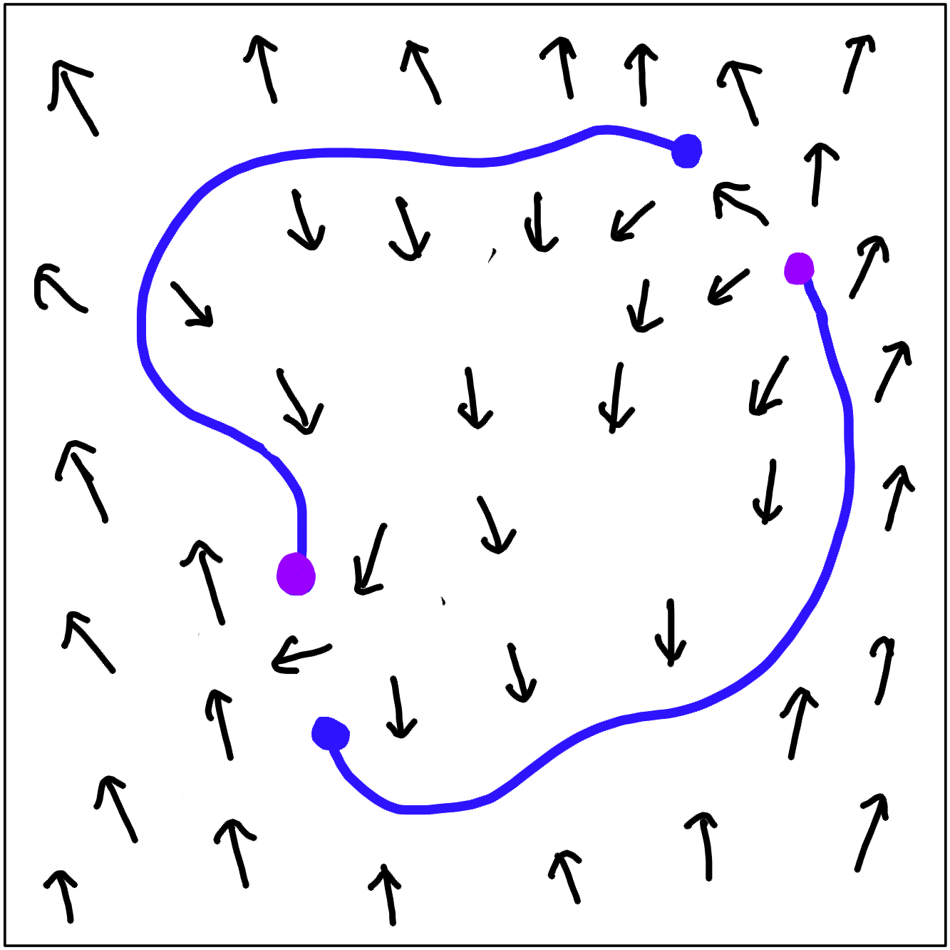
Figure 6: A configuration of XY spins in a modified XY model, with 1/2-vortices (dots) that are connected by strings (blue) where the phase (indicated by arrows) jumps by $\simeq\pi$. A repair algorithm for the strings allows additional correlators to be defined.

It is interesting to consider repairing one-dimensional lines, for example in 2D.

Refs. [42, 43, 44, 45] analysed a modified Hamiltonian for the 2D classical XY model, in which the interaction energy for a pair of adjacent spins $i$ and $j$ has two minima, one at relative angle ${\theta_{i}-\theta_{j}=0}$, and one at ${\theta_{i}-\theta_{j}=\pi}$:

$$\beta H=-\sum_{\left\langle ij\right\rangle}\left[\Delta\cos\left(\theta_{j}-\theta_{j}\right)+J\cos\left(2(\theta_{j}-\theta_{i})\right)\right].$$ (20)

When $J$ and $\Delta$ are both large, this model has quasi-long-range-order for $e^{i\theta}$ (the superfluid phase). If $\Delta$ is now decreased (still at large $J$), the energy cost of certain string excitations, across which $\theta$ jumps by $\pi$, is decreased — see Fig. 6. In the limit of infinite $J$ these strings are closed, while at finite $J$ they can terminate at half-vortices (Fig. 6). Varying $\Delta$ at fixed large $J$, we may cross a phase transition at which the strings proliferate. This is a transition from the superfluid into a pair superfluid, where $e^{i\theta}$ is disordered (thanks to the strings, across which $e^{i\theta}$ changes sign) but $e^{2i\theta}$ has quasi-long-range order [44].

The simplest picture for this transition is to neglect the half-vortices, since at large $J$ they appear only in bound pairs. Then the strings are treated as closed loops, and are analogous to Ising domain walls. As a result, the phase transition at large $J$ (between superfluid and pair superfluid) has Ising exponents [42, 43]. There are also interesting phase transitions at smaller $J$ [44, 45].

This and similar 2D models could be studied from the “patching” point of view of the present paper, explicitly repairing the loops with an algorithm that pairs (matches) nearby half-vortices, and adds a corresponding segment to the string. Assuming that this repair process is sufficiently local, it would for example allow the Ising anomalous dimension $\eta=1/4$ to be measured directly using a (nonlocal) correlation function, despite the fact that there is no local operator with this anomalous dimension in this theory.

Note that the emergence of closed (unoriented) loops here implies the emergence of a $\mathbb{Z}_{2}$ symmetry. If one direction is viewed as time, this is the conservation of the number of loop segments, modulo 2.

It would be interesting, both in the above case and in the standard XY model/Coulomb gas, to study the relation between the thermodynamic binding/unbinding of vortices, and the success or failure of a given algorithm in finding a quasi-local pairing of vortices and antivortices.

VI.4 Application to experiments in quantum devices

So far we have discussed $\mathbb{Z}_{2}$ gauge theory in the language of 3D classical statistical mechanics. But this gauge theory also describes the quantum statistical mechanics of the simplest $\mathbb{Z}_{2}$ spin liquids/topologically ordered states in two dimensions, including the toric code [46, 47, 48, 49, 50, 51, 19].

Recently it was possible to realize the toric code ground state experimentally [52, 53]. A key question is how to efficiently detect deconfinement in experiments of this type by using measurements of the spins. One approach is the Fredenhagen-Marcu order parameter, which involves a ratio of correlation functions of “bare” Wilson line operators [24, 20, 22]. However this involves measuring exponentially small quantities (because of nonuniversal short-distance effects close to the Wilson line), implying a signal-to-noise problem in the large size limit. Therefore we suggest that an effective method may be instead to directly define emergent string correlators by applying the configuration “repair” idea of Ref. [14] to 2D quantum measurements, rather than 3D Monte Carlo data. Below we give a schematic indication.

After this work was completed, we learned of a related proposal for detecting topological order from 2D quantum measurement snapshots in Ref. [54] (where an RG-inspired procedure for annihilating anyons is used, rather than minimal-weight matching).

A complete measurement of all the qubits making up the quantum state, say in the $\sigma_{x}$ basis, gives a 2D configuration $\{\sigma_{x}\}$. (This configuration is of course random, according to Born’s rule, even though we assume that the initial wavefunction is prepared deterministically.) This configuration is equivalent to a single 2D slice through the 3D configurations discussed above. Since we only have 2D information, the problem of “repairing” the configurations is different to that discussed above, although the general idea is similar.

For idealised wavefunctions (e.g. the toric code), such a measurement gives a $\sigma_{x}$ configuration that can be viewed as a collection of closed loops (i.e. electric flux lines) in the plane. In this setting, the value of a magnetic string operator $V_{P}(\{\sigma_{x}\})$ can be defined in a standard way for a given $\sigma_{x}$ configuration. The definition is the planar version of that in Sec. II.2: each electric flux line that is crossed by $P$ contributes a minus sign to $V_{P}(\{\sigma_{x}\})$. The average of this operator for long path $P$ be used to distinguish the deconfined from the confined phase [19] [point (ii) in Sec. III.4]. Here, averaging requires repeatedly measuring independent instances of the wavefunction.

For a more generic wavefunction the $\sigma_{x}$ configurations obtained by measurement will not form closed loops. However, if we are sufficiently close to the idealized limit, we can define emergent string operator measurements via

$$\widetilde{V}_{P}(\{\sigma_{x}\})\equiv V_{P}(\{\overline{\sigma}_{x}\}),$$ (21)

where $\{\overline{\sigma}_{x}\}$ is a repaired configuration in which dangling-end defects are eliminated. The annihilation of pairs of defects is a standard idea in error correction [55]: in the most basic standard algorithm, $\overline{\sigma}_{x}$ is obtained from $\sigma_{x}$ by flipping a minimal set of spins that removes all dangling ends. This geometrical algorithm is used here for a different purpose, namely to define functions $\widetilde{V}_{P}(\{\sigma_{x}\})$ for any configuration.

At first glance, having defined $\widetilde{V}_{P}(\{\sigma_{x}\})$, we can now use expectation values of $\widetilde{V}_{P}(\{\sigma_{x}\})$ (averaged over complete measurements of many instances of the state) to demonstrate deconfinement in the same way as in the idealized case.

However, it is necessary to first verify that the repair process gives a sufficiently local operator ${\widetilde{V}_{P}(\{\sigma_{x}\})}$. In the three-dimensional case, we were able to analyze the locality properties of the patching using percolation concepts and to confirm that patching succeeds all the way up to the Higgs phase boundary. We leave it for the future to analyse the locality of this two-dimensional repair process.

VII Outlook

This paper advocates patching as constructive way of understanding emergent higher symmetries and as a useful tool in simulations. (For example, dimensionless “Binder cumulants” of the dual order parameter may be used to accurately locate the transition.)

We have focused on the case of a simple lattice gauge theory, but patching and its generalizations could be used to construct emergent string operators and dual order parameters in much more general models. It would be interesting to make further numerical explorations. Sec. VI has discussed some examples including models of membranes in the spatial continuum, a generalized XY model, and quantum simulations of topological states.

A key question in any patching scheme is the locality of the patching process. In the patching algorithm that we use, each “hole” (loop) is patched separately. As a result, the locality properties of the algorithm are analyzable using standard ideas from geometrical phase transitions, showing that nontrivial emergent line operators can be constructed in the entirety of the part of the phase diagram where they are expected to exist in the IR.

This loop-by-loop patching scheme is different from a “minimal weight” algorithm, which would find the minimal-area set of patches consistent with a given set of loops. One issue with the latter algorithm is that it involves an optimization problem that may be highly nonlocal even in a configuration where all loops are finite. The locality properties of such a patching procedure would therefore require further analysis.

Gauge fixing in the minimal gauge [2] is closely related to minimal-weight patching (in the appropriate membrane ensemble). In a finite system it differs in the way global excitations are treated. Let us comment on this briefly. The relevant membrane ensemble for gauge fixing is the magnetic ensemble, which is dual to the one we have primarily discussed. Loosely speaking, the relation is that, after gauge fixing, the domain walls of the gauge-fixed Higgs field configuration $\tau^{\text{gauge-fixed}}_{i}$ (cf. Eq. 1) define a configuration $\mathcal{M}_{1}$ of closed membranes. In an infinite system, these are precisely the membranes that are obtained by “patching” an initial configuration of (possibly open) membranes defined by the values of ${\sigma_{ij}\tau_{i}\tau_{j}}$, using a minimal-weight algorithm. In the finite system, however, the configuration $\mathcal{M}_{1}$ can differ from the (minimal-weight) patched configuration $\overline{\mathcal{M}}$ by system-spanning membranes. As a result, the gauge fixing procedure does not in general give access to the operators $\widetilde{V}_{P}$ in the finite periodic system. However, in the infinite-system limit, minimal-gauge-fixing corresponds to a certain choice of patching scheme.

Inside the deconfined phase, there are two emergent one-form symmetries, related by e–m duality. One of these symmetries survives at the Higgs transition, and the dual symmetry survives at the confinement transition. The present approach only gives access to one set of string operators at a time, because it is necessary to pick a basis (electric or magnetic) in order to formulate the partition function as a membrane ensemble. The phase diagram of the standard $\mathbb{Z}_{2}$ gauge theory has an exact self-duality, so it is straightforward to change between the two bases. For more general models (e.g. models in the spatial continuum) the analog of this basis change may be more nontrivial.

Finally let us discuss the multicritical point in Fig. 1. In addition to the confinement and Higgs transition lines, the phase diagram of the gauge theory contains a self-dual multicritical point (MCP) where they meet. The MCP is not yet understood as a conformal field theory, and is an interesting target for further study.

Since the MCP is the meeting point of two critical lines with Ising exponents, at first sight a natural guess would be that it has XY exponents [20]. More recently, this has been argued by Ref. [27], on the basis of the numerical similarity of exponents observed in Ref. [14]. However, challenges to this theoretical interpretation were discussed in Refs. [14, 28]. To begin with, the fixed point associated with the MCP cannot be the fixed point of the XY model (for example because the adjacent phases do not match). In addition, the MCP cannot be an orbifold of the XY fixed point (i.e. an “XY^∗ transition”) as this would not give the correct universal properties of the topologically ordered phase immediately adjacent to the MCP [14].

Ref. [28] has directly demonstrated (using simulations) that there is no U(1) current operator at the MCP CFT, showing that the MCP does not have an emergent global U(1) symmetry. By contrast, the usual “XY^∗” transition has a U(1) symmetry.

These observations do not rigorously exclude the possibility that the exponents of the MCP could be equal to exponents from XY. But (as observed in [14]) if this was the case, it would have to be due to an entirely new type of relationship between conformal field theories, and at present we are not aware of any proposed mechanism. Therefore at present the simplest hypothesis is that the exponents of the MCP are simply numerically close to those of the XY model.

In this paper we have focussed mainly on the part of the phase diagram where the “hole size” $\ell(x,y)$ is finite, so that patching allows a duality to a model with a local order parameter. This works for the confinement transition (as well as in the deconfined phase). The equivalent process works for the Higgs transition, in the dual representation. But at the multicritical point (where Higgs and confinement lines meet), $\ell$ diverges. As a result, patching does not give a duality to a model with a local order parameter at the MCP. This is another reason why, a priori, we do not expect a Landau-like description of the MCP.

Appendix A Scaling arguments

A.1 Lengthscales close to the self-dual MCP

The multicritical point lies on a self-dual line in the phase diagram. Choosing the phase diagram coordinates $(y,y^{\prime})$ where

$$y^{\prime}\equiv\frac{1-x}{1+x},$$ (22)

self duality acts as

$$y\longleftrightarrow y^{\prime}.$$ (23)

Self-duality (which can be treated as a global $\mathbb{Z}_{2}$ symmetry in the infra-red) can be used to classify operators at the MCP. There is an RG relevant, self-duality-preserving operator denoted $S$, with scaling dimension $x_{S}\sim 1.5$, and an RG relevant self-duality-odd (anti-self-dual) operator denoted $A$, with scaling dimension $x_{A}\sim 1.22$ [14]. Writing ${\delta y=y-y_{\text{MCP}}}$, the corresponding perturbations of the MCP are ${\lambda_{+}\equiv\delta y+\delta y^{\prime}}$ and ${\lambda_{-}\equiv\delta y^{\prime}-\delta y}$, respectively, and their RG eigenvalues are ${3-x_{S,A}}$. We let ${\nu_{S,A}\equiv(3-x_{S,A})^{-1}}$.

Turning on a $\lambda_{+}$ perturbation with $\lambda_{+}<0$ leads to the deconfined phase, while turning on $\lambda_{-}$ leads to either the confined or the Higgs state, depending on $\operatorname{sign}\lambda_{-}$. By standard RG results, the shape of the confinement and Higgs phase transition lines, close to the MCP, are given by

$$\lambda_{-}\sim\pm|\lambda_{+}|^{\nu_{S}/\nu_{A}},$$ (24)

so roughly

$$\lambda_{-}\sim\pm|\lambda_{+}|^{1.2}.$$ (25)

Therefore the confinement and Higgs phase transition lines are asymptotically parallel as they approach the MCP, but this cusp behaviour is rather weak since the above exponent is not much larger than 1.

Note that a crude way to obtain the above is to define lengthscales

$$\xi_{\pm}\equiv|\lambda_{\pm}|^{-\nu_{S,A}},$$ (26)

which are the scales at which a given perturbation would renormalize to an order 1 value (in the absence of the other perturbation). The phase transition lines occur where $\xi_{+}$ and $\xi_{-}$ are of the same order (otherwise one of the two perturbations dominates, and we end up in the interior of one of the phases).

Therefore at a point on the confinement phase transition line, but close to the MCP, we have a large lengthscale ${\ell\sim\xi_{+}\sim\xi_{-}}$. Since, on the confinement line, we have (from Eq. 24)

$$\lambda_{+}=2\,\delta y+\mathcal{O}(\lambda_{+}^{\nu_{S}/\nu_{A}}),$$ (27)

this lengthscale is

$$\ell(y)\sim(y_{\text{MCP}}-y)^{-\nu_{S}}.$$ (28)

This is the characteristic lengthscale for the crossover from the universality class of the MCP to universality class of the Ising^∗ confinement transition. (Analogous statements apply for the crossover on the Higgs line.) $\ell(y)$ is also the lengthscale associated with patches, i.e. the scale beyond which larger patches become exponentially rare.

A.2 Fractal structure of patches

When $\ell\gg 1$ we have large patches. We now give scaling arguments using ideas from geometrical critical phenomena (see e.g. Ref. [57]) for (i) the typical area of a large patch and (ii) the moments of the total area of all patches.

First, consider a single large patch whose boundary “loop” (link cluster) has linear size $l$. The total length of this loop — total number of “occupied links” making up the cluster — scales as $l^{d_{f}}$ with

$$d_{f}=1.77(2).$$ (29)

Therefore within a ball of volume $l^{3}$ centred on the centre of mass (CM) of the loop, the average density of occupied links is $\sim l^{d_{f}-3}$. Approximating the distribution of occupied links within this volume as uniform, the number of occupied links within a spherical shell of thickness $\mathrm{d}r$ at radius $r$ scales as $N(r)\mathrm{d}r=l^{d_{f}-3}r^{2}\mathrm{d}r$.

Recall that, to define the patch (Sec. III.2), we first associate a triangle with each occupied link. This triangle connects the link to the loop’s centre of mass. Any link of the dual lattice that pierces an odd number of triangles then gives rise to one of the plaquettes in the patch.

Let $N_{\text{dual}}(r^{\prime})\mathrm{d}r^{\prime}$ be the number of dual links that lie within the spherical shell with radii ${[r^{\prime},r^{\prime}+\mathrm{d}r^{\prime}]}$ and which pierce an odd number of triangles. The density of patched plaquettes is then ${\rho_{\text{patch}}(r^{\prime})=N_{\text{dual}}(r^{\prime})/r^{\prime 2}}$.

To compute $N_{\text{dual}}(r^{\prime})$, we add up contributions from different triangles, associated with occupied links at various possible radii $r$ (where $r^{\prime}<r\lesssim l$). To begin with we neglect double-counting, i.e. the possibility of a dual link piercing more than one triangle. This will be valid in a range $r^{\prime}\gg r_{c}$ where $\rho_{\text{patch}}(r^{\prime})\ll 1$. The scale $r_{c}$ defines a “dense core”, within which different triangles “overlap”, double-counting cannot be neglected, and $\rho_{\text{patch}}(r^{\prime})$ is of order 1. However, $r_{c}\ll l$, so the dense core has a subleading effect on the total area of the patch.

Consider a triangle associated with an occupied link at radius $r$. Since the triangle gets thinner towards the CM, the part of it that lies within the shell ${[r^{\prime},r^{\prime}+\mathrm{d}r^{\prime}]}$ (with $r^{\prime}<r$) has area $\sim(r^{\prime}/r)\mathrm{d}r^{\prime}$, and on average is pierced by order $(r^{\prime}/r)\mathrm{d}r^{\prime}$ dual links within the shell ${[r^{\prime},r^{\prime}+\mathrm{d}r^{\prime}]}$. That is, a triangle whose outer edge is at radius $r$ typically makes a contribution $\sim(r^{\prime}/r)\mathrm{d}r^{\prime}$ to $N_{\text{dual}}(r^{\prime})\mathrm{d}r^{\prime}$.

Adding up such contributions,

$$N_{\text{dual}}(r^{\prime}) \sim\int_{r^{\prime}}^{l}\mathrm{d}rN(r)(r^{\prime}/r)$$ (30)

$$=l^{d_{f}-3}r^{\prime}\int_{r^{\prime}}^{l}\mathrm{d}r\,r$$ (31)

$$\sim l^{d_{f}-1}r^{\prime}H(r^{\prime}/l),$$ (32)

where $H(x)\rightarrow 1$ for $x\ll 1$ and $H(x)\rightarrow 0$ for ${x\gg 1}$. (In our caricature, where the density is uniform, ${H(x)=[1-x^{2}]}$, but this is not accurate.) This gives the density

$$\rho_{\text{patch}}(r^{\prime})={l^{d_{f}-1}}H(r^{\prime}/l)/r^{\prime}.$$ (33)

So far we have neglected double counting. From (33) we see that the radius of the dense core, within which $\rho_{\text{patch}}$ is cut off at an order 1 value, is

$$r_{c}\sim l^{d_{f}-1}\sim l^{0.77(2)}.$$ (34)

Since this exponent is smaller than one, the size of the dense core is much smaller than the total size of the patch, $r_{c}\ll l$. Integrating the density, we find that the typical area of a patch of linear size $l$ is

$$A(l) \sim l^{d_{f}+1}\left(1-\mathcal{O}(l^{-2(2-d_{f})})\right)$$ (35)

$$\sim l^{2.77}\left(1-\mathcal{O}(l^{-0.46})\right),$$ (36)

where the subleading correction is due to the dense core. (In principle there will be other sources of subleading corrections, e.g. due to irrelevant corrections to scaling, that we have not considered.)

Next, consider the total patched area in a membrane configuration. We begin with the MCP, where there are clusters on all scales up to the system size $L$.

For a crude picture, think of $A_{\text{patched}}$ as a sum over contributions from clusters on a range of lengthscales $l_{\tau}=2^{\tau}$ for ${\tau=1,\ldots,\log_{2}L}$:

$$A_{\text{patched}}=\sum_{\tau=1}^{\tau_{\text{max}}}\sum_{i=1}^{n_{\tau}}A^{(\tau)}_{i}.$$ (37)

Here $i$ indexes the clusters at a given scale and $n_{\tau}$ is the number of clusters at a given scale. A caricature that captures the scaling is imagine dividing up the system into $l_{\tau}$-sized blocks, and to think of $n_{\tau}$ as a sum of roughly independent contributions, each of size $\mathcal{O}(1)$, from each block (in reality these contributions are not independent, but that will not matter for the following). We have

$$n_{\tau}\sim(L/l_{\tau})^{3}.$$ (38)

Using (35) above for the typical size $A(l)$ of a patch, we have for the average

$$\frac{\left\langle A_{\text{patched}}\right\rangle}{3L^{3}}\sim (3L^{3})^{-1}\sum_{\tau=1}^{\log_{2}L}(L/l_{\tau})^{3}A(l_{\tau})$$ (39)

$$\sim \alpha-\beta L^{-(2-d_{f})}$$ (40)

as stated in the main text. (The $\alpha$ term is dominated by UV contributions.) If $\ell$ is finite and ${1\ll\ell\ll L}$ then the sum will instead be cutoff at ${l_{\tau}\sim\ell}$, so that the subleading term is of order ${\ell^{-(2-d_{f})}=(y_{\text{MCP}}-y)^{\nu_{S}(2-d_{f})}}$:

$$\lim_{L\rightarrow\infty}\frac{\left\langle A_{\text{patched}}\right\rangle}{3L^{3}}=\alpha-\gamma(y_{\text{MCP}}-y)^{0.15}+\ldots$$ (41)

Writing higher moments of $A_{\text{patched}}$ as a similar sum over scales suggests that they are instead dominated by the largest patches, which are of scale $L$. There are $\mathcal{O}(1)$ patches of this scale with area and fluctuations of order $A(L)$, so that

$$\langle\langle A_{\text{patched}}^{k}\rangle\rangle\sim A(L)^{k}\sim L^{k(d_{f}+1)}.$$ (42)

Moving along the confinement line away from the MCP slightly, a standard rescaling argument gives a scaling form in terms of the crossover scale $\ell$ in Eq. 28:

$$\langle\langle A_{\text{patched}}^{k}\rangle\rangle\sim L^{k(d_{f}+1)}F^{(k)}(L/\ell).$$ (43)

The above carries over straightforwardly to the scaling close to the Higgs line (rather than the MCP) where $\ell$ also diverges, but with the usual Ising correlation length exponent $\nu_{\text{Ising}}$, and where the loops have a distinct fractal dimension (that of Ising worldlines, $d_{f}^{\prime}=1.7349(65)$ [58]). We can also consider a more general point in the vicinity of the MCP, in which case the scaling functions depend not just on $L/\ell$ but on $L/\xi_{+}$ and $L/\xi_{-}$ (Eq. 26) separately.

A.3 Note on locality of $\widetilde{V}_{P}$

We give slightly more detail on the discussion of the local truncation of $\widetilde{V}_{P}$ in Sec. V.1.

Consider the closed path case. The exponential suppression of loops of size $R\gg\ell(x,y)$ means that if we thicken the tube to a scale $R$ (with ${\ell\ll R\ll L}$), the probability that there is a loop pierced by $P$ which we fail to include in the tube is less than ${ALe^{-R/\ell^{\prime}(x,y)}}$ (where $\ell^{\prime}(x,y)$ is proportional to $\ell(x,y)$ when they are both large, and $A$ is a constant). Therefore in order to have a probability of error that is less than $\epsilon$, it is sufficient to take

$$R>\ell^{\prime}(x,y)\,\ln\left(\frac{AL}{\epsilon}\right).$$ (44)

This means that we can approximate $\widetilde{V}_{P}$ with an operator $\widetilde{V}^{\epsilon}_{P}$ that is a function only of the plaquettes inside a tube of radius $R$. These operators agree in a configuration with high probability, so their correlation functions are also approximately equal.

References

- Wegner [1971] F. J. Wegner, Duality in generalized ising models and phase transitions without local order parameters, Journal of Mathematical Physics 12, 2259 (1971).
- Fradkin and Shenker [1979] E. Fradkin and S. H. Shenker, Phase diagrams of lattice gauge theories with higgs fields, Physical Review D 19, 3682 (1979).
- Lammert et al. [1993] P. E. Lammert, D. S. Rokhsar, and J. Toner, Topology and nematic ordering, Physical review letters 70, 1650 (1993).
- Senthil and Motrunich [2002] T. Senthil and O. Motrunich, Microscopic models for fractionalized phases in strongly correlated systems, Physical Review B 66, 205104 (2002).
- Grover and Senthil [2010] T. Grover and T. Senthil, Quantum phase transition from an antiferromagnet to a spin liquid in a metal, Physical Review B 81, 205102 (2010).
- Misguich and Mila [2008] G. Misguich and F. Mila, Quantum dimer model on the triangular lattice: Semiclassical and variational approaches to vison dispersion and condensation, Physical Review B 77, 134421 (2008).
- Moessner and Sondhi [2001] R. Moessner and S. L. Sondhi, Ising models of quantum frustration, Physical Review B 63, 224401 (2001).
- Slagle and Xu [2014] K. Slagle and C. Xu, Quantum phase transition between the z 2 spin liquid and valence bond crystals on a triangular lattice, Physical Review B 89, 104418 (2014).
- Nussinov and Ortiz [2009] Z. Nussinov and G. Ortiz, A symmetry principle for topological quantum order, Annals of Physics 324, 977 (2009).
- Kapustin and Thorngren [2017] A. Kapustin and R. Thorngren, Higher symmetry and gapped phases of gauge theories, in Algebra, Geometry, and Physics in the 21st Century (Springer, 2017) pp. 177–202.
- Gaiotto et al. [2015] D. Gaiotto, A. Kapustin, N. Seiberg, and B. Willett, Generalized global symmetries, Journal of High Energy Physics 2015, 172 (2015).
- Wen [2019] X.-G. Wen, Emergent anomalous higher symmetries from topological order and from dynamical electromagnetic field in condensed matter systems, Physical Review B 99, 205139 (2019).
- Hastings and Wen [2005] M. B. Hastings and X.-G. Wen, Quasiadiabatic continuation of quantum states: The stability of topological ground-state degeneracy and emergent gauge invariance, Physical review b 72, 045141 (2005).
- Somoza et al. [2021] A. M. Somoza, P. Serna, and A. Nahum, Self-dual criticality in three-dimensional z 2 gauge theory with matter, Physical Review X 11, 041008 (2021).
- Iqbal and McGreevy [2022] N. Iqbal and J. McGreevy, Mean string field theory: Landau-ginzburg theory for 1-form symmetries, SciPost Physics 13, 114 (2022).
- McGreevy [2023] J. McGreevy, Generalized symmetries in condensed matter, Annual Review of Condensed Matter Physics 14, 57 (2023).
- Cherman and Jacobson [2023] A. Cherman and T. Jacobson, Emergent 1-form symmetries, arXiv preprint arXiv:2304.13751 (2023).
- Pace and Wen [2023] S. D. Pace and X.-G. Wen, Exact emergent higher-form symmetries in bosonic lattice models, Physical Review B 108, 195147 (2023).
- Kitaev [2003] A. Y. Kitaev, Fault-tolerant quantum computation by anyons, Annals of Physics 303, 2 (2003).
- Huse and Leibler [1991] D. A. Huse and S. Leibler, Are sponge phases of membranes experimental gauge-higgs systems?, Physical review letters 66, 437 (1991).
- Gujrati [1989] P. Gujrati, Critical behavior of n→ 0 gauge-invariant theory: Self-avoiding random surfaces, Physical Review B 39, 2494 (1989).
- Gregor et al. [2011] K. Gregor, D. A. Huse, R. Moessner, and S. L. Sondhi, Diagnosing deconfinement and topological order, New Journal of Physics 13, 025009 (2011).
- Kogut [1979] J. B. Kogut, An introduction to lattice gauge theory and spin systems, Reviews of Modern Physics 51, 659 (1979).
- Fredenhagen and Marcu [1986] K. Fredenhagen and M. Marcu, Confinement criterion for qcd with dynamical quarks, Physical review letters 56, 223 (1986).
- Vidal et al. [2009] J. Vidal, S. Dusuel, and K. P. Schmidt, Low-energy effective theory of the toric code model in a parallel magnetic field, Physical Review B 79, 033109 (2009).
- Tupitsyn et al. [2010] I. Tupitsyn, A. Kitaev, N. Prokof’Ev, and P. Stamp, Topological multicritical point in the phase diagram of the toric code model and three-dimensional lattice gauge higgs model, Physical Review B 82, 085114 (2010).
- Bonati et al. [2022] C. Bonati, A. Pelissetto, and E. Vicari, Multicritical point of the three-dimensional gauge higgs model, Physical Review B 105, 165138 (2022).
- Oppenheim et al. [2023] L. Oppenheim, M. Koch-Janusz, S. Gazit, and Z. Ringel, Machine learning the operator content of the critical self-dual ising-higgs gauge model, arXiv preprint arXiv:2311.17994 (2023).
- Balian et al. [1974] R. Balian, J. Drouffe, and C. Itzykson, Gauge fields on a lattice. i. general outlook, Physical Review D 10, 3376 (1974).
- Binder [1981] K. Binder, Critical properties from monte carlo coarse graining and renormalization, Physical Review Letters 47, 693 (1981).
- Kos et al. [2016] F. Kos, D. Poland, D. Simmons-Duffin, and A. Vichi, Precision islands in the ising and o (n) models, Journal of High Energy Physics 2016, 36 (2016).
- Katzgraber [2009] H. G. Katzgraber, Introduction to monte carlo methods, arXiv preprint arXiv:0905.1629 (2009).
- Vanderzande [1992] C. Vanderzande, Fractal dimensions of potts clusters, Journal of Physics A: Mathematical and General 25, L75 (1992).
- Jacobsen et al. [2003] J.-L. Jacobsen, N. Read, and H. Saleur, Dense loops, supersymmetry, and goldstone phases in two dimensions, Physical review letters 90, 090601 (2003).
- Huse and Leibler [1988] D. A. Huse and S. Leibler, Phase behaviour of an ensemble of nonintersecting random fluid films, J. Phys. (Paris) 49, 605 (1988).
- Cates et al. [1988] M. Cates, D. Roux, D. Andelman, S. Milner, and S. Safran, Random surface model for the l3-phase of dilute surfactant solutions, EPL (Europhysics Letters) 5, 733 (1988).
- Roux et al. [1990] D. Roux, M. Cates, U. Olsson, R. Ball, F. Nallet, and A. Bellocq, Light scattering from a surfactant “sponge” phase: Evidence for a hidden symmetry, EPL (Europhysics Letters) 11, 229 (1990).
- Roux et al. [1992] D. Roux, C. Coulon, and M. Cates, Sponge phases in surfactant solutions, The Journal of Physical Chemistry 96, 4174 (1992).
- Roux [1995] D. Roux, Sponge phases: An example of random surfaces, Physica A: Statistical Mechanics and its Applications 213, 168 (1995).
- [40] L. Peliti, “amphiphilic membranes”, in “fluctuating geometries in statistical mechanics and field theory”, f. david, p. ginsparg, j. zinn-justin, (eds.) les houches, session lxii, 1994 (amsterdam: Elsevier, 1996) 195-285.
- Lipowsky [1991] R. Lipowsky, The conformation of membranes, Nature 349, 475 (1991).
- Korshunov [1985] S. Korshunov, Possible splitting of a phase transition in a 2d xy model, JETP Lett 41 (1985).
- Lee and Grinstein [1985] D. Lee and G. Grinstein, Strings in two-dimensional classical xy models, Physical review letters 55, 541 (1985).
- Shi et al. [2011] Y. Shi, A. Lamacraft, and P. Fendley, Boson pairing and unusual criticality in a generalized x y model, Physical review letters 107, 240601 (2011).
- Serna et al. [2017] P. Serna, J. Chalker, and P. Fendley, Deconfinement transitions in a generalised xy model, Journal of Physics A: Mathematical and Theoretical 50, 424003 (2017).
- Read and Chakraborty [1989] N. Read and B. Chakraborty, Statistics of the excitations of the resonating-valence-bond state, Physical Review B 40, 7133 (1989).
- Kivelson [1989] S. Kivelson, Statistics of holons in the quantum hard-core dimer gas, Physical Review B 39, 259 (1989).
- Read and Sachdev [1991] N. Read and S. Sachdev, Large-n expansion for frustrated quantum antiferromagnets, Physical review letters 66, 1773 (1991).
- Wen [1991] X.-G. Wen, Mean-field theory of spin-liquid states with finite energy gap and topological orders, Physical Review B 44, 2664 (1991).
- Senthil and Fisher [2000] T. Senthil and M. P. Fisher, Z 2 gauge theory of electron fractionalization in strongly correlated systems, Physical Review B 62, 7850 (2000).
- Moessner et al. [2001] R. Moessner, S. L. Sondhi, and E. Fradkin, Short-ranged resonating valence bond physics, quantum dimer models, and ising gauge theories, Physical Review B 65, 024504 (2001).
- Satzinger et al. [2021] K. Satzinger, Y.-J. Liu, A. Smith, C. Knapp, M. Newman, C. Jones, Z. Chen, C. Quintana, X. Mi, A. Dunsworth, et al., Realizing topologically ordered states on a quantum processor, Science 374, 1237 (2021).
- Bluvstein et al. [2022] D. Bluvstein, H. Levine, G. Semeghini, T. T. Wang, S. Ebadi, M. Kalinowski, A. Keesling, N. Maskara, H. Pichler, M. Greiner, et al., A quantum processor based on coherent transport of entangled atom arrays, Nature 604, 451 (2022).
- Cong et al. [2022] I. Cong, N. Maskara, M. C. Tran, H. Pichler, G. Semeghini, S. F. Yelin, S. Choi, and M. D. Lukin, Enhancing detection of topological order by local error correction, arXiv preprint arXiv:2209.12428 (2022).
- Dennis et al. [2002] E. Dennis, A. Kitaev, A. Landahl, and J. Preskill, Topological quantum memory, Journal of Mathematical Physics 43, 4452 (2002).
- Schmaltz [1999] M. Schmaltz, Duality of nonsupersymmetric large n gauge theories, Physical Review D 59, 105018 (1999).
- Stauffer and Aharony [2018] D. Stauffer and A. Aharony, Introduction to percolation theory (Taylor & Francis, 2018).
- Winter et al. [2008] F. Winter, W. Janke, and A. M. Schakel, Geometric properties of the three-dimensional ising and x y models, Physical Review E 77, 061108 (2008).