Enhancing chest X-ray datasets with privacy-preserving large language models and multi-type annotations: a data-driven approach for improved classification

Abstract

In chest X-ray (CXR) image analysis, rule-based systems are usually employed to extract labels from reports, but concerns exist about label quality. These datasets typically offer only presence labels, sometimes with binary uncertainty indicators, which limits their usefulness. In this work, we present MAPLEZ (Medical report Annotations with Privacy-preserving Large language model using Expeditious Zero shot answers), a novel approach leveraging a locally executable Large Language Model (LLM) to extract and enhance findings labels on CXR reports. MAPLEZ extracts not only binary labels indicating the presence or absence of a finding but also the location, severity, and radiologists’ uncertainty about the finding. Over eight abnormalities from five test sets, we show that our method can extract these annotations with an increase of 5 percentage points (pp) in F1 score for categorical presence annotations and more than 30 pp increase in F1 score for the location annotations over competing labelers. Additionally, using these improved annotations in classification supervision, we demonstrate substantial advancements in model quality, with an increase of 1.7 pp in AUROC over models trained with annotations from the state-of-the-art approach. We share code and annotations.

table longtable

1 Introduction

Multi-label classification of chest X-ray (CXR) images has been widely explored in the computer vision literature. Publicly available large datasets, including CheXpert [20], NIH ChestXray14 [53] and MIMIC-CXR [24], provide CXR images as well as the corresponding labels for several common findings or diagnoses. Given the scale of the datasets, the labels used for training the CXR classifiers are typically extracted from radiology reports using either traditional natural language processing tools, such as the CheXpert labeler [20] and the Medical-Diff-VQA labeler [18, 61], or deep learning based tools, such as CheXbert [43].

Unfortunately, these tools are imperfect, and the labels are often noisy [16]. Consequently, medical imaging classification models performed better when humans annotated labels directly from the CXR than when using the report annotations from those tools [16]. One of the ways of reducing that gap without needing expert review of hundreds of thousands of images is to improve the ability of the labeler to create annotations from reports.

Recently, general-purpose pre-trained large language model (LLM) such as GPT4 [35], Llama [50] or Vicuna [6] have been shown to be effective at labeling radiology reports [1, 32, 30]. A key advantage of these LLM tools is that they have good performance without additional training or finetuning. Additionally, using LLMs with publicly available weights, such as Llama or Vicuna, allows one to run these models locally (on-premise) without risking patients’ privacy. It is also not always possible to include anonymized data provided by public datasets in prompts to cloud-based LLM. For example, to comply with the MIMIC-CXR data use agreement, the use of cloud LLMs with the reports of that dataset is limited to a particular cloud service setup that might not be available to every researcher [37]. Finally, the United States government has shown that it considers the development of privacy-preserving data analytics tools a priority [10]

Another improvement that can be made to labelers is to extract more detailed information from the reports than just whether a given finding is present, absent, or not mentioned in a report. For instance, in a concurrent work, the rule-based Medical-Diff-VQA labeler [18, 61] has been used to extract multi-type annotations: presence mentions, relative changes from previous reports, location, uncertainty, and severity of abnormalities from CXR reports.  Hu et al. [18] and Zhang et al. [61] showed an advantage of using some of these types of annotations when training classifiers.

Our hypothesis in this paper is twofold:

• the extraction of several types of annotations from CXR reports can be improved by developing a labeler employing a locally-run LLM;

• these annotations can train a CXR image classifier that outperforms models trained using competing labelers.

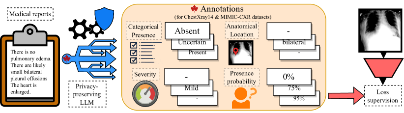
Fig. 1: Representation of the MAPLEZ project. A knowledge-driven decision tree prompt system for a privacy-preserving LLM labels medical reports for several abnormalities with four types of annotations: categorical presence, presence probability, severity, and anatomical location. We used MAPLEZ to annotate two publicly available CXR datasets, making annotations with higher quality than competing labelers. We then showed the advantages of employing the annotations for training a CXR classifier.

Therefore, we propose the MAPLEZ labeler based on the SOLAR-0-70b-16bit LLM. It uses a knowledge-driven decision tree prompt system to process medical reports and produce four types of abnormality annotations: presence, probability of presence, anatomical location, and severity. A representation of the MAPLEZ method is presented in 1. We produce and share MAPLEZ’s annotations for the MIMIC-CXR [24] and NIH ChestXray14 [53]. We show the superiority of the MAPLEZ method against competing labelers in three annotation types. In addition to those datasets, we evaluate the prompt system for a limited set of reports from other medical imaging modalities. We propose using the new annotations and a multi-task loss to supervise a classification model of a CXR. Our findings show that the annotations lead to significant improvement in classification performance.

Key Contributions

• Providing a zero-shot fast prompt system for annotation extraction in medical reports in the form of prompts and open-source code, which other researchers can adapt to their research needs.

• Providing improved and extended annotations (presence, probability, location, and severity) for two of the largest CXR datasets, MIMIC-CXR [24] and NIH ChestXray14 [53]. These annotations could be used, for example, in detection and visual question-answering tasks.

• Performing extensive evaluation of the annotations to show their superior quality against other commonly employed report labelers.

• Showing that the method can be easily adapted to reports from other medical imaging modalities: we present high F1 scores of the proposed labeler on PET, CT, and MRI reports.

• Proposing methods of employing the new multi-type annotations and showing quality improvements of an image classifier when using such methods and annotations.

1.1 Related works

1.1.1 Using large language models to extract report labels

Few works employ privacy-preserving LLMs to extract medical report labels.  Khosravi et al. [26] performed a small-scale experiment to show that a privacy-preserving LLM could provide good labeling for one specific abnormality from CT reports.  Mukherjee et al. [32] showed that a privacy-preserving LLMs performed on par with rule-based labelers for CXR reports. Our work develops a more complex prompt system and performs extensive experiments to show that a privacy-preserving LLM can actually perform better than rule-based labelers.

Adams et al. [1] did a preliminary study showing that GPT-4 provided abnormality category labels on par with a state-of-the-art deep learning tool, whereas  [30] showed a better performance by the GPT family of LLMs. Both works only processed hundreds of reports for their experiments without having to deal with making the prompt system tractable for several abnormalities, annotation types, and hundreds of thousands of reports.

A recent concurrent work by Gu et al. [15] used GPT-4 to label 50,000 reports for 13 abnormalities from the MIMIC-CXR dataset. They then trained a deep learning model on those automated ground truths for classifying the presence or absence of the findings based on the reports. We judge that the F1 scores in their results in the categorical label annotation are similar to what we present in our paper. However, their method is less quickly adaptable to new labels and modalities since their prompt is not zero-shot, and producing a new labeler requires tens of thousands of example reports to be evaluated by GPT-4 and another round of training for CheXbert. In contrast, our method requires only the replacement of abnormality names in the prompt system.

With the exception of the works from Mukherjee et al. [32] and Liu et al. [30], the extraction of categorical abnormality presence employing LLMs has been limited to binary presence or absence. In contrast, the more fuzzy approach of our method can highlight the uncertainties of the noisy labels extracted directly from reports. Furthermore, to our knowledge, we are the first to demonstrate significant downstream classification task improvements with labels from an LLM-based labeler compared to employing annotations from previous state-of-the-art labeler tools.

1.1.2 Extracting structured multi-type annotations from reports

LesaNet [57] was trained on a CT dataset that contained 171 labels, several of which characterized the location or severity of the abnormality. These labels were extracted with a rule-based labeler only from sentences that contained lesion bookmarks, probably causing several false negatives from attributes present in other sentences of the report.  Zhang et al. [61] used a CXR report rule-based labeler to extract the same four types of annotations as we propose to extract with MAPLEZ: categorical presence, probability of presence, severity, and location of abnormalities. They also extracted labels characterizing the comparison of previous reports, which we did not extract. However, we show in our results that LLMs perform significantly better than their rule-based labeler and argue that our proposed method is much more adaptable than a rule-based system, which requires a list of all the possible wording of mentions of each type of abnormality. To our knowledge, our work is the first to use LLMs to generate report annotations for numerical probability, severity, and location of abnormalities.

1.1.3 Extracting labels from PET, CT, and MRI reports

Stember and Shalu [44] (MRI),  Wood et al. [55] (MRI),  Wood et al. [56] (MRI),  Iorga et al. [19] (CT),  Zech et al. [59] (CT),  Titano et al. [48] (CT),  Schrempf et al. [38] (CT),  Schrempf et al. [39] (CT),  Bressem et al. [5] (CT), and  Grivas et al. [14] (CT, MRI) developed supervised machine learning systems for labeling binary presence of specific types of abnormalities in medical reports after manually labeling thousands of reports for supervision.  D’Anniballe et al. [9] (CT) extracted  Draelos et al. [11] (CT),  Yan et al. [57] (CT),  [14] (CT, MRI), and  Bradshaw et al. [4] (PET) developed rule-based systems for extracting presence of abnormalities from reports. The existence of so many labeling systems with their own annotated supervision data or set of rules suggests that there is no single established tool for extracting abnormality labels from PET, CT, or MRI reports. These reports contain a more diverse set of abnormalities reported than CXR reports, so the lack of easy adaptability of rule-based and supervised machine learning systems probably significantly impacts the use of these developed tools in subsequent research.

Shin et al. [41] provided a more generic approach to labeling CT, MRI, and PET reports: they extracted sentences containing reference images (e.g., (Series 1001, image 32)) from hundreds of thousands of reports and processed those sentences with an unsupervised natural language processing clustering method to create 80 classes of abnormality presents in the reports. In opposition to this approach, MAPLEZ does not require a vast corpus of reports to be developed and does not have the restriction of only working for sentences with reference images.  Khosravi et al. [26] presented a small-scale experiment to show that LLMs could be employed to extract the presence of one specific abnormality from CT reports. Unlike their method, our method provides fuzzy and multi-type annotations, and our paper performs a more extensive analysis of the adaptability and the quality of the labels generated by LLMs.

2 Methods

2.1 A Prompt system for automatic annotation of CXR reports

To enhance the quality of annotations derived from CXR reports, we use the SOLAR-0-70b-16bit LLM [51, 54], which is accessible to the public under the CC BY-NC-4.0 license. This model adapts the Llama 2 model [50], further finetuned on two unspecified instruction datasets similar to broadly-employed datasets [29, 33, 31, 47]. We chose this model after, at the start of the project, we tested several openly available LLMs, including medical LLMs.

We did not modify or finetune the LLM, employing it in a zero-shot manner. Our custom-designed prompt system takes a radiologist’s report and generates annotations for the 13 abnormalities listed in Section A.1.2. These 13 abnormality labels were selected from CheXpert [20], the most known baseline. A new set of labels would complicate comparison experiments, leading to additional label translations. However, as shown in this paper, our method is easily adaptable to other abnormality labels.

We focused on extracting four specific annotation categories for each abnormality: categorical presence, probability of presence, severity, and anatomical location. To improve our prompts, we experimented on a validation set with 100 manually annotated reports from the NIH ChestXray14 dataset [53]. Initial testing with tailored prompts revealed that querying the LLM about specific abnormalities yielded more precise responses than multiple abnormalities simultaneously. Furthermore, we observed that chain-of-thought prompts [27] were impractical for processing 227,827 CXRs reports from the MIMIC-CXR dataset [24] for 13 types of abnormalities and four annotation categories due to computation time. To enhance efficiency, we used prompts that demanded brief responses, typically up to four tokens in length, significantly reducing computational demands.

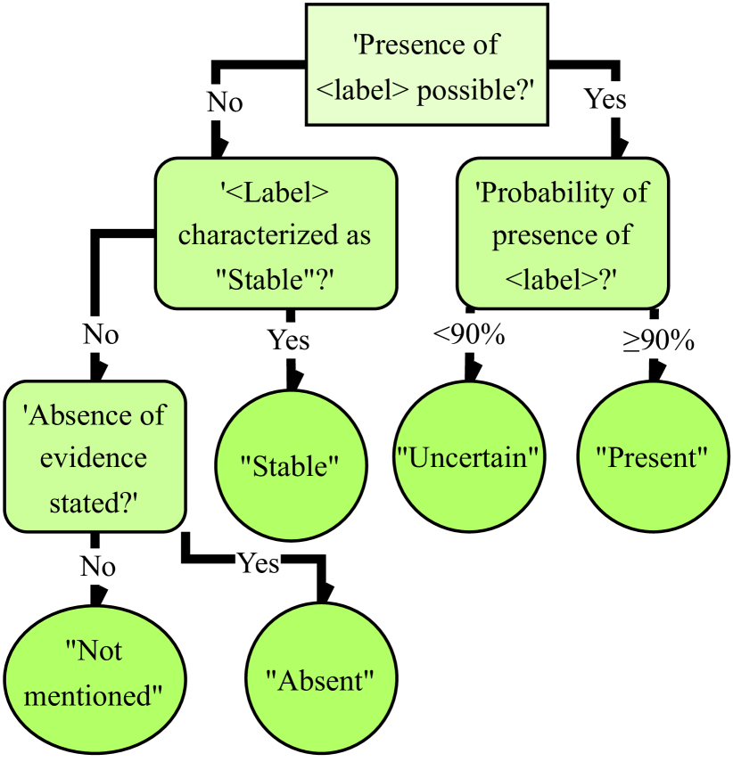
(a) Categorical presence decision tree

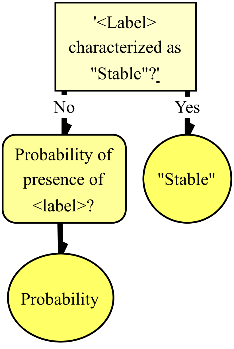
(b) Probability decision tree

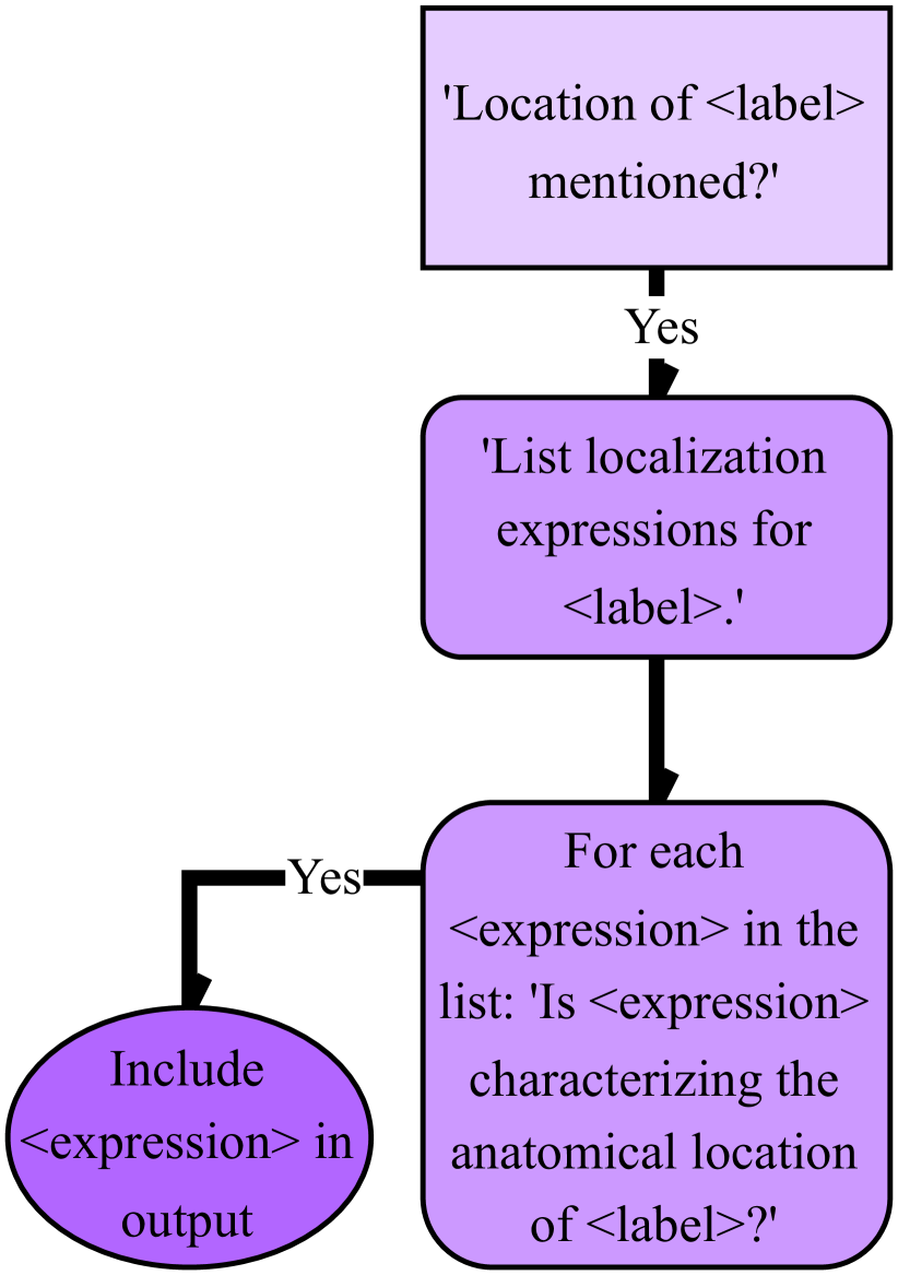
(c) Location decision tree

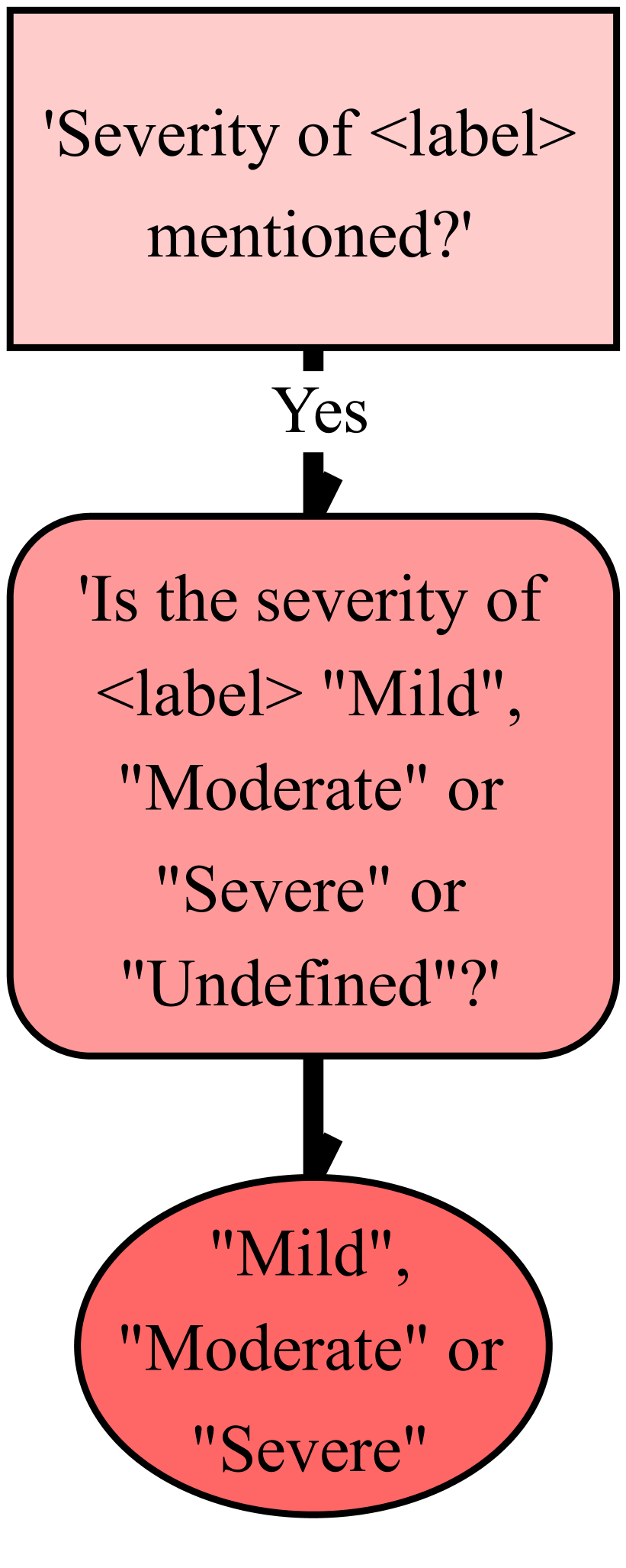
(d) Severity decision tree

Fig. 2: Simplified representation of the knowledge-driven decision tree prompt system and its possible outputs. The location and severity knowledge-driven decision trees are only run when the abnormality is labeled as “Uncertain” or “Present”.

We implemented a knowledge-based decision tree prompt system to guide the annotation process. Simplified visual representations of this system can be found in Fig. 2, with the full prompts detailed in Section Section A.1. The five possible outputs for the categorical presence of an abnormality were “Present”, “Absent”, “Not mentioned”, “Uncertain”, i.e., the radiologist expresses uncertainty about the abnormality being present (radiologist uncertainty), or “Stable”, i.e., the radiologist compares the state of an abnormality to the state from a previous report without indicating its presence or not (text uncertainty). We diverged from the CheXpert labeler’s practice of assigning the same category to “Uncertain” and “Stable” cases, opting for distinct categories to allow for their separate handling. Upon establishing the possible presence of an abnormality, the LLM checks if the report includes details on location or severity. For severity annotations, the LLM outputs one of three categories: “Mild”, “Moderate”, or “Severe”. For location annotations, the LLM is instructed to enumerate the characterizing locations, separating them with semi-colons. Listing the locations is the only prompt requiring a lengthy response in our labeler. Subsequently, the LLM verifies each listed location to ensure they describe anatomical locations. For the probability annotations, the model either categorizes the abnormality as “Stable” or outputs a probability between 0% and 100%.

We observed an improvement in performance on our prompt experimentation set when we expanded abnormality denominations – the way different abnormalities are mentioned in our prompts – to include synonyms and subtypes, which were based on the rules of the CheXpert labeler [21]. The text we used as abnormality denominations in the prompts can be found in Section A.1.2.

2.2 Merging abnormality subtypes

Some abnormalities are a merge of subtypes of that abnormality. Specifically, we categorize “Consolidation” as a blend of “Consolidation” and “Pneumonia”, while “Lung opacity” merges several conditions: “Atelectasis”, “Consolidation”, “Pneumonia”, “Edema”, “Lung lesion”, and “Lung opacity” itself. When combining these conditions, we define “Consolidation” and “Lung opacity” as primary labels. Our methodology for integrating the diagnostic labels varies by the type of label:

• for presence labels, we prioritize them as follows: “Present” is prioritized over “Uncertain,” which is prioritized over “Stable,” which in turn is prioritized over “Absent” (if it is a primary label), followed by “Not mentioned,” and lastly “Absent.” (if it is not a primary label);

• for probability labels, we combine abnormalities by using the highest probability, with “Stable” prioritized over probabilities less than or equal to 50%;

• for severity labels, we apply a similar highest-value approach, treating the absence of abnormality or severity as the lowest priority severity level;

• for location labels, we concatenate the different locations into one list, ensuring there are no duplicates.

2.2.1 Adapting the system to other medical imaging modalities

To test its adaptability, we made minor modifications to run MAPLEZ with other types of medical text: CT, MRI, and PET reports. We changed the selection of abnormalities to contain the ones usually mentioned in those reports, and we did not validate the abnormality denominations. The abnormality labels and denominations are presented in Section A.1.2. The rest of the prompt system was the same, except for a mention of the modality of the report, replacing Given the (complete/full) report excerpts with Given the (complete/full) <modality>  report, where <modality>  was ct, mri, or pet.

2.3 Employing the new annotations

We trained a convolutional neural network (CNN) CXR classifier using the annotations obtained with the LLM. Out of the 13 available abnormalities, we focused on eight to standardize the outputs of our approach and baseline methods. The classifier was trained to detect abnormalities with supervision from categorical or probabilistic annotations. The binary cross-entropy loss was employed in both cases, and the probabilities were used as soft labels. Additionally, we explored leveraging severity and anatomical location annotations as additional supervision in a multi-task loss.

We selected anatomically significant keywords with non-overlapping meanings to allow the classifier to learn from the location annotations. Our selection involved analyzing the most frequent n-grams in the annotations across different abnormality groups. The chosen keywords, such as right, left, and lower, are listed in Section A.2.1. We also identified terms in the annotations that were synonymous with some keywords and created a replacement-word list; for instance, the presence of bilateral in an annotation would indicate both left and right keyword labels were positive. The complete list of these replacement words is in Section A.2.1.

Determining negative keyword labels for each case posed a challenge. We decided on a rule: a label is negative only if mutually exclusive with a positive label. For example, if right is positive, left becomes negative, but lower remains unaffected since an abnormality in the left lung might be in the lower left lung. Additionally, anatomically adjacent terms prevented each other from being labeled as negative. For example, if lower and upper are positive, base will not be negative, even though it is mutually exclusive with upper: lower being anatomically close to base will prevent that. Full details of these relationships are shown in Section A.2.1. Any keywords not categorized as positive or negative for an abnormality are treated as unlabeled and ignored in the location loss calculation.

Our model’s architecture included distinct logit outputs for each selected location keyword of each abnormality. We calculated the location loss using binary cross-entropy for each logit, integrating it into the overall loss function by multiplying it with a weighting factor, $\lambda_{loc}$, and adding it to the presence classification loss.

Lastly, we experimented with the severity labels from Medical-Diff-VQA and MAPLEZ labelers. We only applied a scaled multi-class cross-entropy loss when a severity annotation was available. However, this modification did not yield improvements in the area under the ROC curve (AUROC) on our validation set, so we do not detail this aspect further.

3 Results

3.1 Labeler evaluation

For evaluating the LLM annotations in CXR reports, we hand-labeled categorical presence, severity and location of abnormalities for 350 reports from the MIMIC-CXR dataset [13, 24, 23] and 200 reports from the NIH ChestXray14 dataset [53]. Details about these hand annotations are given in Section A.3.1. We also used public datasets that were labeled by radiologists directly from the CXR images:

• REFLACX [3, 2, 13]: phase 3 of the REFLACX dataset has 2,507 frontal CXRs from the MIMIC-CXR dataset [24] labeled for several abnormalities by a single radiologist among five radiologists. Phases 1 and 2 of the same dataset have 109 frontal CXRs, each labeled by five radiologists. We used these two phases for the inter-observer scores for Table 2. The dataset also includes probabilities assigned by radiologists to each abnormality. The probability labels are annotated using five categories, and we convert them to probability intervals: “Absent”: $[0\%,5\%]$; “Unlikely (<10%)”: $[0\%,15\%]$; “Less Likely (25%)”: $[10\%,40\%]$; “Possibly (50%)”: $[35\%,65\%]$; “Suspicious for/Probably (75%)”: $[60\%,90\%]$; “Consistent with (>90%)”: $[85\%,100\%]$. We selected five abnormalities from this dataset that were equivalent to the ones from the CheXpert labeler [20]. One of the five abnormalities was a merge from several labels, as shown in Paragraph A.3.2.1, following the merging rules from Section 2.2.

• Pneumonia: the RSNA Pneumonia Detection Challenge (2018) dataset [40] contains 26,684 CXR studies from the NIH ChestXray14 dataset [53], each labeled for presence of pneumonia/consolidation by one to three radiologists from a set of 18 radiologists.

• Pneumothorax: the dataset from the National University Hospital from Singapore [16] contains 24,709 studies from the NIH ChestXray14 dataset [53] labeled for the presence of pneumothorax by one of four radiologists.

Table 1: F1 scores ($\uparrow$) for five labelers for the categorical presence annotation. MAPLEZ is our proposed method, and CheXpert, Vicuna, and Medical-Diff-VQA (VQA) are the competing methods. These symbols represent the p-values from the two-sided bootstrap hypothesis test for difference in median between the score of MAPLEZ and the other scores in that specific table row: ^∗∗∗ for p<0.001, ^∗∗ for p<0.01, ^∗ for p<0.05, and ^ns for not significant. Precision, recall, confidence intervals, and aggregations by abnormality are presented in LABEL:tab:labelsfull. NIH=NIH ChestXray14 dataset [53]; MIMIC=MIMIC-CXR dataset [24]; RFL-3= phase 3 of the REFLACX dataset [3]; PNA=Pneumonia dataset [40]; PTX=Pneumothorax dataset [16]; Abn.=Abnormality; Atel.=“Atelectasis”; Card.=“Cardiomegaly”; Cons.=“Consolidation”; Fract.=“Fracture”; Opac.=“Lung opacity”; Effus.=“Pleural Effusion”; PTX=“Pneumothorax”; N=total labeled test cases; N⁺=number of positive cases for that abnormality; W=weight used in the aggregation of dataset scores, related to the variance of the score; MAPLEZ-G=MAPLEZ-Generic, the model that uses simpler abnormality denominations in its prompts; Human=aggregation for all datasets labeled by radiologists straight from the CXRs, which are marked with italic.

Data	Abn.	$N$	$N^{+}$	W	CheXpert	Vicuna	VQA	MAPLEZ-G	MAPLEZ (Ours)
NIH	Atel.	200	27	0.009	0.909ns	0.852ns	-	0.871ns	0.820
MIMIC	Atel.	350	104	0.061	0.832∗∗∗	0.935ns	0.950ns	0.942ns	0.951
NIH	Card.	200	21	0.003	0.647∗∗	0.774∗	-	0.837ns	0.955
MIMIC	Card.	350	132	0.029	0.735∗∗∗	0.873∗	0.757∗∗∗	0.939ns	0.932
RFL-3	Card.	506	171	0.007	0.447∗∗∗	0.585ns	0.463∗∗∗	0.616ns	0.616
NIH	Cons.	200	70	0.003	0.533∗∗∗	0.506∗∗∗	-	0.604∗∗∗	0.952
MIMIC	Cons.	350	90	0.019	0.838ns	0.728∗∗	0.846ns	0.843ns	0.882
RFL-3	Cons.	506	154	0.004	0.454ns	0.343∗∗∗	0.441ns	0.466ns	0.509
PNA	Cons.	7186	2589	0.072	0.381∗∗∗	0.414∗∗∗	-	0.517∗∗∗	0.633
NIH	Edema	200	15	0.001	0.786ns	0.621ns	-	0.526ns	0.688
MIMIC	Edema	350	111	0.022	0.848ns	0.746∗	0.844ns	0.815ns	0.839
RFL-3	Edema	506	115	0.006	0.468ns	0.548ns	0.498ns	0.548ns	0.552
MIMIC	Fract.	350	20	0.001	0.516∗	0.552∗	0.833ns	0.872ns	0.842
NIH	Opac.	200	122	0.045	0.892ns	0.818∗∗∗	-	0.896ns	0.923
MIMIC	Opac.	350	262	0.128	0.878∗∗∗	0.885∗∗	0.899∗	0.917ns	0.938
RFL-3	Opac.	506	342	0.066	0.785ns	0.790ns	0.772ns	0.796ns	0.796
NIH	Effus.	200	60	0.025	0.857∗	0.852∗∗	-	0.914ns	0.961
MIMIC	Effus.	350	134	0.118	0.926ns	0.942ns	0.929ns	0.951ns	0.962
NIH	PTX	200	26	0.008	0.915ns	0.686∗	-	0.931ns	0.882
RFL-3	PTX	506	16	0.000	0.250ns	0.500ns	0.333ns	0.526ns	0.483
PTX	PTX	24709	2912	0.373	0.758ns	0.586∗∗∗	-	0.770ns	0.756
NIH	-	-	-	-	0.877∗∗∗	0.812∗∗∗	-	0.891∗∗∗	0.926
MIMIC	-	-	-	-	0.875∗∗∗	0.895∗∗∗	0.901∗∗∗	0.923ns	0.939
RFL-3	-	-	-	-	0.752∗∗∗	0.765∗	0.744∗∗∗	0.772ns	0.773
Human	-	-	-	-	0.691∗∗∗	0.630∗∗∗	-	0.720∗∗∗	0.732
All	-	-	-	-	0.810∗∗∗	0.784∗∗∗	-	0.847∗∗∗	0.860

In tests, we compared MAPLEZ against four labelers:

• CheXpert [20]: we ran this labeler on the MIMIC-CXR dataset [24] and the test set of the NIH dataset [53]. It was only compared in the categorical presence task.

• Medical-Diff-VQA [61]: the annotations only included the MIMIC-CXR dataset [24], so this labeler does not have results for some of the experiments. The labeler provides categorical presence, probability expressions, location expressions, and severity words. Probability expressions were converted to percentages with a conversion table. Severity words were converted to severity classes using the rules from our manual labeling of the MIMIC-CXR and NIH ChestXray14 ground truths. We also grouped a few abnormalities of the dataset using the rules described in Section 2.2. The grouped abnormalities and the probability and severity conversion rules are presented in Paragraph A.3.2.2.

• Vicuna [32]: we employed its annotations for the test sets of the MIMIC-CXR [24] and NIH [53] datasets. It was only compared in the categorical presence task.

• MAPLEZ-Generic: MAPLEZ-Generic is a version of our labeler using simpler abnormality denominations without synonyms or subtypes of each abnormality. The abnormality denomination strings for MAPLEZ and MAPLEZ-Generic are presented in Section A.1.2.

For all four types of annotations, we computed precision, recall, and the F1 score for eight abnormalities common for the five labelers. More details about these calculations and complete tables are presented in Section B. We calculated a weighted average for score aggregations using the minimum variance unbiased estimator. We provide more weighted average calculation details in Section A.7 and the employed weights in the respective result tables.

Table 2: F1 scores ($\uparrow$) for categorical presence annotations for two radiologists (Rad.) and our proposed method in phases 1 and 2 of the REFLACX dataset [3], with $N=109$. The ground truth was the majority vote of the other three radiologists. LABEL:tab:humansfull is a complete version of this table, with precision, recall, and confidence intervals. Refer to Table 1 for a list of abbreviation meanings.

Abn.	$N^{+}$	W	Rad.	MAPLEZ
Card.	30	0.11	0.456ns	0.600
Cons.	33	0.09	0.451ns	0.492
Edema	13	0.02	0.222ns	0.343
Opac.	65	0.78	0.730ns	0.784
All	-	-	0.695∗	0.757

Results for the categorical presence annotations are presented in Table 1. When processing labeler outputs and ground truths, we considered “Uncertain” as “Present” and “Stable” as “Absent”. To compare the F1 scores against humans, we present Table 2, which contains scores of one radiologist against the majority vote of 3 radiologists.

To evaluate probability annotations, we used the probability labels set by radiologists on the REFLACX dataset [3]. We calculated the mean absolute error (MAE) to get numerical results between the predicted probabilities and the radiologist ground truth. We considered “Stable” probabilities from MAPLEZ as 0%. Results are presented in Table 3. Radiologists’ performance is presented in Table 20.

Table 3: Aggregated results for three of the tested tasks. The full results, with precision, recall, confidence intervals, and subdivision by abnormality, are presented in Tables 19, LABEL:tab:locationfull and LABEL:tab:severityfull. The location and severity tasks had a varying $N$ depending on the evaluated abnormality. The caption of Table 1 presents the meaning of abbreviations and symbols.

Task	Score	Dataset	N	VQA [61]	MAPLEZ-G	MAPLEZ (Ours)
Probability	MAE ($\downarrow$)	RFL-3	506	25.3 [23.8,26.8]∗	22.9 [21.6,24.2]ns	22.0 [20.7,23.3]
Location	F1 ($\uparrow$)	MIMIC	-	0.538 [0.493,0.580]∗∗∗	0.815 [0.789,0.842]∗	0.866 [0.843,0.888]
Severity	F1 ($\uparrow$)	MIMIC	-	0.784 [0.701,0.850]ns	0.753 [0.667,0.826]ns	0.712 [0.629,0.784]

To evaluate the labeling of the location of abnormalities, we considered F1 scores for the presence of location keywords instead of full location expressions. These results are presented in Table 3. Keywords and replacement words are listed in Section A.2.2. Severity annotations were evaluated by considering any severity present as a positive label. Details about the location and severity score calculations and further results are presented in Sections A.6 and B, in LABEL:tab:severityfull and LABEL:tab:severityall. Severity and location annotations were evaluated only on the MIMIC-CXR dataset to allow the comparison with the Medical-Diff-VQA method.

To evaluate the adaptation of the prompt system to other modalities, we labeled 40 CT, 40 MRI, and 39 PET reports for categorical presence and, except for PET, location. A senior radiologist specializing in abdominal imaging chose the abnormality categories employed for each modality. The location keywords employed for this evaluation are presented in Section A.2.2, and the replacement list was the same as for the CXR reports. The results are presented in Table 4.

Table 4: F1 scores ($\uparrow$) for the MAPLEZ annotations for reports of modalities other than CXR. For precision, recall, confidence intervals, and subdivision by abnormality, check LABEL:tab:othermodalitiesfull and 18.

Data	CT	MRI	PET	All
Presence	0.889	0.884	0.833	0.873
Location	0.843	0.805	-	0.830

3.2 Classifier evaluation

We compared a model trained with MAPLEZ annotations against two baselines: one trained with the Medical-Diff-VQA labeler [61] annotations and one trained with the CheXpert labeler [20] annotations. All used annotations and reports were from the MIMIC-CXR dataset [24]. A comparison of the statistics of the annotations from each labeler is provided in Section A.3. A complete list of tested hyperparameters and employed training parameters and architectures for all methods is presented in Section A.5.

We evaluated our classification results only on datasets for which the ground truth annotations were labeled by radiologists directly from the CXR. In addition to the datasets presented in Section 3.1, we also employed the test set of the CheXpert [20] dataset, which contains 500 CXR studies labeled each by majority vote from 5 radiologists among a set of 8 radiologists. Three of the four employed test datasets contain images from other CXR datasets not seen during training: NIH ChestXray14 [53] and CheXpert [20]. We also did an ablation study to evaluate the impact of modifications proposed in this paper: the use of probability annotations instead of categorical presence labels, the multi-task use of location labels, the ignoring of “Stable” abnormality labels, and the inclusion of synonyms in abnormality denominations. These results are presented in Table 5.

Table 5: AUROC scores ($\uparrow$) in four radiologist-labeled datasets for the classifiers we trained. To the left, we compare the classifier trained with annotations from MAPLEZ or its competing labelers. To the right, we show the results of the ablation study, where ‘$\lambda_{loc}=0$’ is trained without the multi-task loss, ‘Cat. Labels’ is trained with categorical labels instead of probability annotations, ‘Use “Stable”’ does not ignore the “Stable” abnormalities, setting them to a 50% probability, ‘MAPLEZ-G’ is the MAPLEZ-Generic model, with simplified abnormality denominations in the prompts, and “All Changes” is the model with all four modifications, and considering “Stable” as “Present”. LABEL:tab:classifierfull is a complete version of this table, subdivided by abnormalities and containing confidence intervals. CXt=CheXpert dataset. Refer to Table 1 for the meaning of other abbreviations and symbols.

Data	CheXpert	VQA	MAPLEZ	$\lambda_{loc}=0$	Cat. Labels	Use “Stable”	MAPLEZ-G	All Changes
PNA	0.793∗∗∗	0.783∗∗∗	0.840	0.833ns	0.834ns	0.839ns	0.845ns	0.819∗∗
PTX	0.920∗∗∗	0.926∗∗	0.937	0.932ns	0.933ns	0.934ns	0.932ns	0.934ns
RFL-3	0.827∗∗∗	0.857ns	0.871	0.871ns	0.870ns	0.873ns	0.869ns	0.850∗
CXt	0.881∗∗∗	0.905∗∗∗	0.933	0.931ns	0.934ns	0.928ns	0.932ns	0.925ns
All	0.890∗∗∗	0.912∗∗∗	0.929	0.925ns	0.926ns	0.927ns	0.925ns	0.920∗∗∗

4 Discussion

With a few exceptions, our proposed method showed better performance than competing methods. In Table 1, our method significantly outperformed the three competing labelers in five non-aggregated rows without being significantly outperformed in any individual rows. Our method outperformed the three competing methods in all dataset aggregations, increasing the F1 scores by 0.029 to 0.050 against the best-performing competing method of each row. Some precision and recall scores might seem relatively low for a medical task. Still, we show in Table 2 that the scores of our method, which annotates CXRs from a radiology report from the MIMIC-CXR dataset, are not significantly worse than the scores of individual radiologists annotating CXRs directly from the image. This lower score for the Human datasets, in which separate radiologists annotated CXR reports and image labels, probably happened because of inter-observer variability. Since manual annotations and extracted labels came from the same report, there was no inter- or intra-observer variability for the NIH ChestXray14 and MIMIC-CXR datasets.

Table 1 shows that the MAPLEZ labeler performed potentially worse than the other labelers in extracting information from reports for the “Edema” abnormality when compared to the ground truth manually labeled from reports. However, it showed potentially better agreement than the other labelers when comparing the annotations against radiologists’ annotations. Therefore, the variability might only be due to random chance. However, according to LABEL:tab:classifierfull, the classifier trained with the MAPLEZ annotations also potentially performed slightly worse on the “Edema” classification task. These additional results corroborate the hypothesis of slightly worse performance for MAPLEZ’s “Edema” labels. We reviewed MAPLEZ’s “Edema” outputs in 20 test mistakes to further understand these scores. False negatives seemed to happen from a combination of the presence of alternative abnormality wording in the reports (vascular congestion, vascular engorgement) and the presence of low probability/severity adjectives in the reports (less likely, minimal if any, without other evidence of). “Edema” false positives happened because the LLM confused enlarged heart with “Edema”, because of complex wording (patient history of edema, interval resolution of edema) and because there were a few incorrect annotations in the test set ground truth.

Table 3 shows that the probabilities outputted by the MAPLEZ method from a radiologist report significantly conform better to probabilities assigned by other radiologists directly to the same CXR than the outputs of the Medical-Diff-VQA method. Even though radiologists are not consistent in their language to express probability [42], the LLM is still able to extract meaningful probabilities and even outperform other radiologists assigning probabilities directly to the CXR, as shown in Table 20.

Our method significantly outperformed the Medical-Diff-VQA method for location annotations, achieving an F1 score of more than 0.300 higher, as shown in Tables 3, LABEL:tab:locationall and LABEL:tab:locationsimple. This superiority even happened when we limited the evaluated vocabulary to only words included in the manual rules of the Medical-Diff-VQA dataset (LABEL:tab:locationsimple). Rule-based location extraction is probably in early development, and its rule set could still be expanded. It does not identify several location expressions (“lateral”, “perihilar” or “fissure”, for example), leading to a low recall. Using an LLM for location expression extraction seems more generalizable in a short development time.

The MAPLEZ labeler achieved an F1 score 0.072 lower than the Medical-Diff-VQA method for severity. Even though the difference was statistically insignificant, this result might show one of our method’s deficiencies. We evaluated severity outputs in 20 test mistakes. False negative errors were caused by a combination of alternative wording not included in the prompt (small, extensive, subtle) and because some severity adjectives were not adjacent to the abnormality mention. False positives were caused by the presence of nearby adjectives characterizing another abnormality and by a few incorrect test set ground truth annotations.

LABEL:tab:labelsfull, LABEL:tab:locationfull, LABEL:tab:locationall and LABEL:tab:locationsimple demonstrate that MAPLEZ outperformed other labelers in the categorical presence and location annotations mainly because of a higher recall. LABEL:tab:severityfull and LABEL:tab:severityall show that MAPLEZ’s relatively lower performance for the severity annotations was caused mainly by a lower precision than other methods.

The MAPLEZ method scored better than the MAPLEZ-Generic method in the location and categorical presence annotation tasks. These results show that adding rule-based aspects to the prompts – the multiple ways of mentioning the same abnormality – can positively impact the labeler. This enhancement likely occurred because the short answers prevented the model from identifying synonyms in some cases, which was remediated by including those in the prompts. However, the fact that the performance of MAPLEZ-Generic, in most cases, was closer to MAPLEZ than to CheXpert, Vicuna, or Medical-Diff-VQA shows that the main advantage of the proposed MAPLEZ method comes from the use of a performant LLM and of a well-validated extensive prompt system. It also shows that the technique will likely perform well when adapted to other abnormalities, even if a careful manual definition of abnormality denominations is not performed.

The scores of our adaptation to other medical modalities achieved in Table 4 are comparable to the scores reached by the MAPLEZ-Generic model in LABEL:tab:locationall and 1. The abnormality denominations were not validated for this adaptation and abnormality synonyms were not included in the prompt. Therefore, it performs similarly to MAPLEZ-Generic, which did not include abnormality synonyms in the prompts. These results show the potential and accessibility of such a tool in facilitating research in various medical imaging projects in other modality types or for a different label set.

As shown in Table 5, the classifier trained with the annotations from the MAPLEZ labeler performed better than the classifiers trained with the annotations of either the CheXpert labeler or the Medical-Diff-VQA labeler in all datasets, with a significant difference in all but one dataset. These results show that the annotations we extracted are more useful in a downstream classification task.

The ablation study from Table 5 shows, without statistical significance, that the method choices of how to employ the data from the MAPLEZ labeler were individually beneficial to the classifier. All changes together had a statistically significant benefit to the classifier. The use of the extracted anatomical location through the location loss ($\lambda_{loc}=0.01$) provides the model with additional supervision, possibly teaching it to focus on the correct area of the CXR when a finding is present. This hypothesis could be tested in future work. The optimal $\lambda_{loc}$ is 0.01 for MAPLEZ’s labels but only 0.001 for the Medical-Diff-VQA dataset. This fact corroborates the proposed labeler’s superiority and lower noise labels against its compared baseline. Employing probability labels instead of categorical labels leads to a better AUROC probably because the model has a more forgiving loss when the radiologist is unsure about an abnormality in complex or dubious cases. Ignoring the cases labeled as “Stable” is probably beneficial because those cases have very noisy labels. For those cases, the information about the abnormality presence is inaccessible to the labeler because it is only listed in a previous CXR report of the same patient. Having fewer training cases (Ignore “Stable”) showed benefits against having more noisy data (Use “Stable”). As shown in Tables 1 and LABEL:tab:locationfull, the MAPLEZ labeler is more accurate than MAPLEZ-Generic, so the use of abnormality synonyms in the LLM prompts leads to a better classifier through less noisy training labels.

4.1 Limitations

Our classifier did not achieve state-of-the-art performance in some tasks. For example, the model trained with radiologist-labeled annotations by Hallinan et al. [16] achieved an AUROC of 0.943 [0.939, 0.946], and the performance of our model was slightly lower than the lower end of that confidence interval. Indeed, our study focused on showing the advantage of using the MAPLEZ labeler instead of achieving the best classifier. During training, for example, we did not use lateral images as inputs, the images of the NIH ChestXray14 dataset (so that experiments were comparable to the Medical-Diff-VQA labeler), or the CheXpert training set. There are also many unexplored ways of integrating the provided annotations into classification models and losses that were not proposed in this paper. Our paper did not offer definitive directions of exploration on how to use the data best since our ablation study failed to show statistical significance when comparing the different proposed data uses individually, even if it was significantly better than when all proposed methods were ablated. Additionally, we did not show any positive impact of using the severity annotations, likely because the annotations for severity were too noisy to be used in supervision.

When other researchers try to adapt the MAPLEZ method to their work needs, defining the appropriate abnormality denominations and local hardware requirements may pose deployment difficulty. However, we showed that simple adaptations to other modalities can achieve results comparable to results that MAPLEZ-Generic achieved for CXRs. For deployment in the future, it is unclear if the same prompt system will be adaptable to a more sophisticated next-generation LLMs since we did not evaluate prompt transferability between LLMs. The procedure of extracting labels from reports and then using them for training a classifier might also become obsolete as there will likely be further development of large multimodal models that learn end-to-end medical tasks involving language and vision.

In future work, when trying to improve the MAPLEZ’s performance in the categorical presence of “Edema” and in severity tasks, alternative wording mistakes could potentially be solved with longer prompts. For example, the abnormality denomination lung edema (CHF or vascular congestion or vascular prominence or indistinctness) could be validated for “Edema”, and including abnormality size or other synonyms could be validated for the severity. Other types of mistakes would probably need a more powerful LLM or a chain-of-thought answer prompt [27]. Other potential improvements for the prompt system are optimizing its computational speed and including a “Normal” category output to fully match the functionalities of the CheXpert labeler.

5 Conclusion

We showed that LLMs can improve the quality of annotation of medical reports and still be run locally without sharing potentially confidential data. We also showed that the answers given by the LLMs can have high quality even if chain-of-thought reasoning is not used. LLMs can also help estimate the uncertainty expressed by radiologists in their reports, which can reduce noise in annotations. The use of LLMs has the potential to expedite medical research by facilitating the extraction of textual information. Compared to rule-based systems, LLMs enable the fast development of strategies for extracting data from texts and, as our findings show, provide annotations with superior quality. Finally, we showed that training modifications made possible by the MAPLEZ method led to significantly improved classification scores for a CXR abnormality detection model.

6 Data and code availability

Part of the anonymized datasets and labelers we used are publicly available: CheXpert labeler [20], CheXpert test set [20], CXRs of the NIH ChestXray 14 dataset [53], and the images/reports of MIMIC-CXR [24]. Other datasets and baseline methods are private and were obtained after anonymization and analyzed with IRB approval. The code for producing these results and the MAPLEZ annotations, the annotations we processed for the complete MIMIC-CXR and NIH ChestXray14 datasets, and the ground truth manual annotations used for part of our evaluation are available at https://github.com/rsummers11/CADLab/tree/master/MAPLEZ_LLM_report_labeler/.

Declaration of generative AI and AI-assisted technologies in the writing process

During the preparation of this work the author(s) used ChatGPT and Grammarly in order to improve writing quality. After using this tool/service, the author(s) reviewed and edited the content as needed and take(s) full responsibility for the content of the publication.

References

A Experimental details

A.1 Prompts

A complete representation of the knowledge-drive decision tree prompt system is given in Figs. 3 and 4. As seen in Fig. 3, the LLM interactions for getting the four types of annotations start with common prompts and branch out to prompts specific to each annotation type. This configuration saves computational time when annotating for all four annotation types simultaneously.

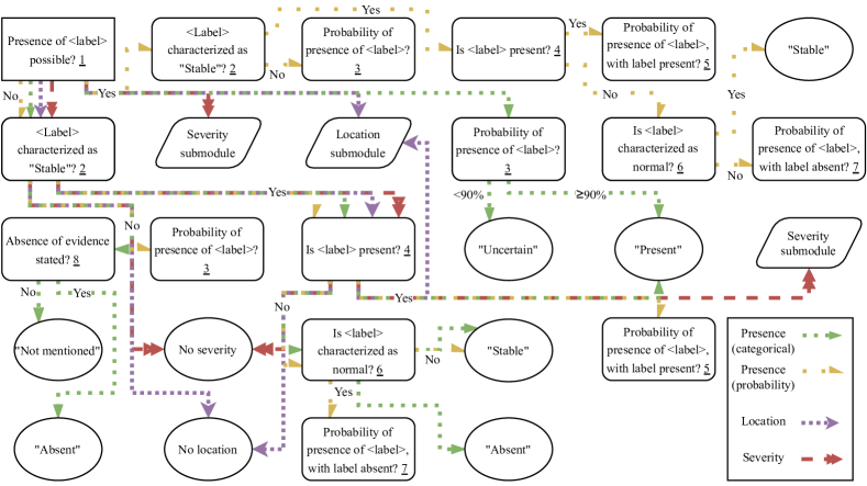
Fig. 3: Full representation of the knowledge-driven decision tree prompt system, except for the exact prompts used. Different arrow styles represent the decision tree and simplified prompts for each of the four types of annotations. Some blocks are submodules whose prompt system is represented in Fig. 4. Questions/prompts are numbered, and their complete respective text prompts are presented in Section A.1.1. For simplicity, probability outputs are not indicated, but they are the LLM answer to each of the probability questions (3, 5, and 7).

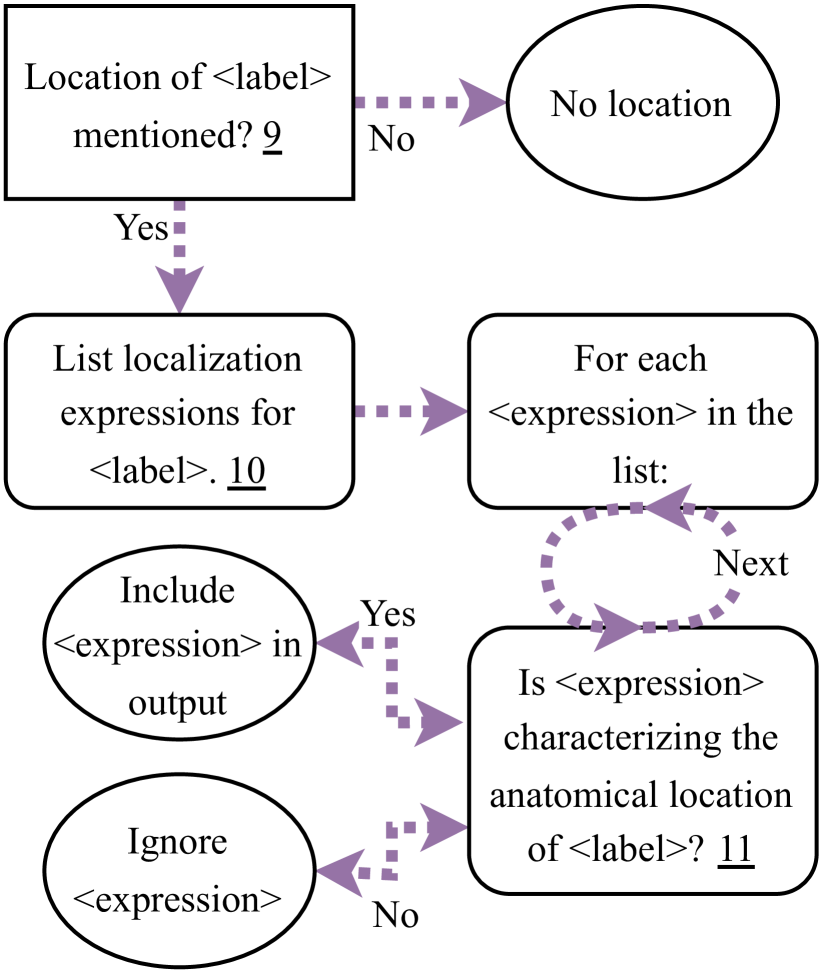
(a) Location submodule

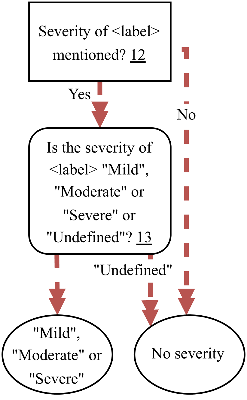
(b) Severity submodule

Fig. 4: Submodules that are indicated in Fig. 3.

A.1.1 Prompt texts

These are the complete prompts used in our knowledge-driven decision tree prompt system:

• 1: Given the full report "<report>", use a one sentence logical deductive reasoning to infer if the radiologist observed possible presence of evidence of "<label>". Respond only with "Yes" or "No".

• 2: For “Enlarged cardiomediastinum” and “Cardiomegaly”, the prompt was: Given the full report "<report>", use a one sentence logical deductive reasoning to infer if the radiologist characterized "<label>" as stable or unchanged. Respond only with "Yes" or "No".. For other labels, the prompt was: Given the full report "<report>", use a one sentence logical deductive reasoning to infer if the radiologist characterized specifically "<label>" as stable or unchanged. Respond only with "Yes" or "No".

• 3: Consider in your answer: 1) radiologists might skip some findings because of their low priority 2) explore all range of probabilities, giving preference to non-round probabilities 3) medical wording synonyms, subtypes of abnormalities 4) radiologists might express their uncertainty using words such as "or", "possibly", "can't exclude", etc… Given the complete report "<report>", estimate from the report wording how likely another radiologist is to observe the presence of any type of "<label>" in the same imaging. Respond with the template "___% likely." and no other words.

• 4: For “Support devices”, the prompt was: Say "Yes".. For other labels, the prompt was: Given the full report "<report>", use a one sentence logical deductive reasoning to infer if "<label>" might be present. Respond only with "Yes" or "No".

• 5: Consider in your answer: 1) radiologists might skip some findings because of their low priority 2) explore all range of probabilities, giving preference to non-round probabilities 3) medical wording synonyms, subtypes of abnormalities 4) radiologists might express their uncertainty using words such as "or", "possibly", "can't exclude", etc… Given the complete report "<report>", consistent with the radiologist observing "<label>", estimate from the report wording how likely another radiologist is to observe the presence of any type of "<label>" in the same imaging. Respond with the template "___% likely." and no other words.

• 6: For “Enlarged cardiomediastinum” and “Cardiomegaly”, the prompt was: Given the full report "<report>", use a one sentence logical deductive reasoning to infer if the radiologist characterized "<label>" as normal. Respond only with "Yes" or "No".. For other labels, the prompt was: Given the full report "<report>", use a one sentence logical deductive reasoning to infer if the radiologist characterized specifically "<label>" as normal. Respond only with "Yes" or "No".

• 7: Consider in your answer: 1) radiologists might skip some findings because of their low priority 2) explore all range of probabilities, giving preference to non-round probabilities 3) medical wording synonyms, subtypes of abnormalities 4) radiologists might express their uncertainty using words such as "or", "possibly", "can't exclude", etc… Given the complete report "<report>", consistent with the radiologist stating the absence of evidence "<label>", estimate from the report wording how likely another radiologist is to observe the presence of any type of "<label>" in the same imaging. Respond with the template "___% likely." and no other words.

• 8: Given the full report "<report>", use a one sentence logical deductive reasoning to infer if the radiologist stated the absence of evidence of "<label>". Respond only with "Yes" or "No".

• 9: Given the complete report "<report>", does it mention a location for specifically "<label>"? Respond only with "Yes" or "No".

• 10: Given the report "<report>", list the localizing expressions characterizing specifically the "<label>" finding. Each adjective expression should be between quotes, broken down into each and every one of the localizing adjectives and each independent localiziation prepositional phrase, and separated by comma. Output an empty list ("[]" is an empty list) if there are 0 locations mentioned for "<label>". Do not mention the central nouns identified as "<label>". Do not mention any nouns that are not part of an adjective. Only include in your answer location adjectives adjacent to the mention of the "<label>" finding. Exclude from your answer adjectives for other findings. Use very short answers without complete sentences. Start the list (0+ elements) of only localizing adjectives or localizing expressions (preposition + noun) right here: [

• 11: Consider in your answer: 1) medical wording synonyms, subtypes of abnormalities 2) abreviations of the medical vocabulary. Given the complete report "<report>", is the isolated adjective "<expression>", on its own, characterizing a medical finding in what way? Respond only with "_" where _ is the number corresponding to the correct answer. (1) Anatomical location of "<label>" (2) Comparison with a previous report for "<label>" (3) Severity of "<label>" (4) Size of "<label>" (5) Probability of presence of "<label>" (6) Visual texture description of "<label>" (7) It is not characterizing the "<label>" mention noun (8) A type of support device Answer:"

• 12: Given the complete report "<report>", would you be able to characterize the severity of "<label>", as either "Mild", "Moderate" or "Severe" only from the words of the report? Respond only with "Yes" or "No".

• 13: Given the complete report "<report>", characterize the severity of "<label>" as either "Mild", "Moderate" or "Severe" or "Undefined" only from the words of the report, and not from comparisons or changes. Do not add extra words to your answer and exclusively use the words from one of those four options.

The underlined number in each item connects the full prompts to the simplified prompts used in Figs. 3 and 4. For the listed prompts, <report> is replaced with the report being analyzed, <label> is replaced with the abnormality denominations listed in Section A.1.2, and <expression> is replaced with one of the expressions listed by the LLM as an answer to question 9. In the reports that were input to the prompt, anonymized words, usually indicated by ____, were replaced by thing. For the MIMIC-CXR dataset, the findings, comparison, and impression sections were included in the input report. Only the findings section was included for the CT, MRI, and PET modalities.

A.1.2 Abnormalities denominations

We followed the definitions of abnormalities from the CheXpert labeler GitHub repository [Irvin et al., 2019b]. The abnormality denominations included a subset of those terms and were chosen with validation experiments after being compared to other CheXpert term subsets. For all 13 abnormalities that our prompt system evaluates, these are the denominations used inside the prompts:

• “Enlarged cardiomediastinum”: enlarged cardiomediastinum (enlarged heart silhouette or large heart vascularity or cardiomegaly or abnormal mediastinal contour)

• “Cardiomegaly”: cardiomegaly (enlarged cardiac/heart contours)

• “Atelectasis”: atelectasis (collapse of the lung)

• “Consolidation”: consolidation or infiltrate

• “Edema”: lung edema (congestive heart failure)

• “Fracture”: fracture (bone)

• “Lung lesion”: lung lesion (mass or nodule)

• “Pleural effusion”: pleural effusion (pleural fluid) or hydrothorax/hydropneumothorax

• “Pneumonia”: pneumonia (infection)

• “Pneumothorax”: pneumothorax (or pneumomediastinum or hydropneumothorax)

• “Support devices”: medical equipment or medical support devices (lines or tubes or pacers or apparatus)

• “Lung opacity”: lung opacity (or decreased lucency or lung scarring or bronchial thickening or infiltration or reticulation or interstitial lung)

• “Pleural other”: pleural abnormalities other than pleural effusion (pleural thickening, fibrosis, fibrothorax, pleural scaring)

For prompts that are exclusively evaluating probability, location, or severity, the following abnormalities had their denominations slightly modified:

• “Support devices”: medical equipment or support device (line or tube or pacer or apparatus or valve or catheter)

• “Pleural other”: fibrothorax (not lung fibrosis) or pleural thickening or abnormalities in the pleura (not pleural effusion)

In Section 3.1, the MAPLEZ-Generic labeler abnormality denominations are simplified to evaluate the importance of adding the synonyms and subtypes to them. These are the simplified denominations used in that case:

• “Enlarged cardiomediastinum”: enlarged cardiomediastinum

• “Cardiomegaly”: cardiomegaly

• “Atelectasis”: atelectasis

• “Consolidation”: consolidation

• “Edema”: lung edema

• “Fracture”: fracture

• “Lung lesion”: lung lesion

• “Pleural effusion”: pleural effusion

• “Pneumonia”: pneumonia

• “Pneumothorax”: pneumothorax

• “Support devices”: medical equipment or support device

• “Lung opacity”: lung opacity

• “Pleural other”: abnormalities in the pleura (not pleural effusion)

In Section 2.2.1, we mentioned the MAPLEZ labeler’s adaptation to other medical reports modalities. A senior radiologist specializing in abdominal imaging selected The CT/MRI/PET labels. These are the denominations that we used in our prompts and the chosen abnormalities for each modality, listed in parenthesis:

• “Lung lesion” (CT): lung lesion;

• “Liver lesion” (CT, MRI): liver lesion;

• “Kidney lesion” (CT, MRI): kidney lesion;

• “Adrenal gland abnormality” (CT, MRI): adrenal gland abnormality;

• “Pleural effusion” (CT): pleural effusion;

• “Hypermetabolic abnormality in the thorax’ (PET): hypermetabolic abnormality in the thorax;

• ’Hypermetabolic abnormality in the abdomen’ (PET): hypermetabolic abnormality in the abdomen;

• ’Hypermetabolic abnormality in the pelvis’ (PET): hypermetabolic abnormality in the pelvis.

A.2 Location keywords

A.2.1 Location keywords for training a classifier

The following words were all of the location category keywords that were selected for employment during the training process for each abnormality:

• “Cardiomegaly”: right, left, upper, lower, base, ventricle, atrium

• “Lung Opacity”:apical, middle, right, left, upper, lower, base, lateral, perihilar, retrocardiac,

• “Edema”:apical, middle, right, left, upper, lower, base, lateral, perihilar, retrocardiac,

• “Consolidation”:apical, middle, right, left, upper, lower, base, lateral, perihilar, retrocardiac,

• “Atelectasis”:apical, middle, right, left, upper, lower, base, lateral, perihilar, retrocardiac,

• “Pneumothorax”:apical, middle, right, left, upper, lower, base, lateral, perihilar, retrocardiac,

• “Pleural Effusion”:apical, middle, right, left, upper, lower, base, lateral, perihilar, retrocardiac,

• “Fracture”:middle, right, left, upper, lower, lateral, posterior, anterior, rib, third, fourth, fifth, sixth, seventh, eighth, ninth, clavicular, spine

These are the words that, when present in the list of free-form text annotated by the model, made each of the keyword categories positive (replacement list):

• right: bilateral, bilaterally, lungs, biapical, apices, apexes, bases, bibasilar, chest walls, ventricles, atriums, clavicles

• left: bilateral, bilaterally, lungs, biapical, apices, apexes, retrocardiac, bases, bibasilar, chest walls, ventricles, atriums, clavicles

• apical:biapical, apices, apexes, apical

• lower:retrocardiac

• middle:mid

• base:basilar, bases, bibasilar

• ventricle:ventricles

• atrium:atriums

• posterior:posterolateral

• lateral:posterolateral

• rib:ribs

• third:3rd, 3

• fourth:4th, 4, four

• fifth:5th, 5, five

• sixth:6th, 6, six

• seventh:7th, 7, seven

• eighth:8th, 8, eight

• ninth:9th, 9, nine

• clavicular:clavicle, clavicles

• spine:vertebrae, vertebra, vertebral

The items of the following list are location keywords that, when positive, prevented the keywords in the associated list on the right from being negative:

• apical: upper,

• middle: upper, lower,

• upper: apical, middle,

• lower: base, retrocardiac, middle, base: saylower, retrocardiac,

• perihilar: atrium, ventricle,

• ventricle: retrocardiac, perihilar, lower, left,

• atrium: retrocardiac, perihilar, lower,

• posterior: rib,

• anterior: rib

• third: rib,

• fourth: rib,

• fifth: rib,

• sixth: rib,

• seventh: rib,

• eighth: rib,

• ninth: rib,

• clavicular: upper, apical,

• spine: perihilar,

• retrocardiac: left, lower, perihilar, base, atrium, ventricle,

The items of the following list are location keywords that, when positive, made the keywords in the associated list on the right negative unless the associated keyword was prevented from being negative (as shown in the list above):

• apical: lower, base, retrocardiac, ventricle, atrium

• middle: apical, base, ventricle, atrium

• right: left, retrocardiac, atrium, ventricle,

• left: right, atrium,

• upper: lower, base, retrocardiac, ventricle, atrium,

• lower: upper, apical, clavicular,

• base: upper, apical, middle,

• lateral: perihilar, retrocardiac, atrium, spine,

• perihilar: lateral,

• ventricle: right, atrium, upper, apical,

• atrium: ventricle, upper, apical, lateral,

• posterior: clavicular, anterior, spine,

• anterior: clavicular, posterior, spine,

• rib: clavicular, spine,

• third: fourth, fifth, sixth, seventh, eighth, ninth, clavicular, spine,

• fourth: third, fifth, sixth, seventh, eighth, ninth, clavicular, spine,

• fifth: third, fourth, sixth, seventh, eighth, ninth, clavicular, spine,

• sixth: third, fourth, fifth, seventh, eighth, ninth, clavicular, spine,

• seventh: third, fourth, fifth, sixth, eighth, ninth, clavicular, spine,

• eighth: third, fourth, fifth, sixth, seventh, ninth, clavicular, spine,

• ninth: third, fourth, fifth, sixth, seventh, eighth, clavicular, spine,

• clavicular: third, fourth, fifth, sixth, seventh, eighth, ninth, spine, rib, lower,

• spine: third, fourth, fifth, sixth, seventh, eighth, ninth, clavicular, rib, lateral,

• retrocardiac: right, lateral, upper, apical,

A.2.2 Location keywords for labeler evaluation

The selection and use of keywords and replacement words are performed similarly to Section 2.3, but also analyzing the ground truth annotations to decide what keywords to use. Furthermore, the vocabulary of location expressions provided by the Medical-Diff-VQA labeler is limited. We built a list of frequent keywords in that dataset and performed evaluation only for those, without allowing for the replacement of words. The considered keywords were: right, left,upper, lower, base, apical, retrocardiac, rib,middle, and results in LABEL:tab:locationsimple.

The following list presents the keywords that were considered location categorical labels when the evaluation of the location outputs of the labelers, presented in Table 3, was calculated:

• “Cardiomegaly”: right, left, upper, lower, base, ventricle, atrium

• “Lung opacity”: apical, middle, right, left, upper, lower, base, lateral, perihilar, retrocardiac

• “Edema”: apical, middle, right, left, upper, lower, base, lateral, perihilar, retrocardiac

• “Consolidation”: apical, middle, right, left, upper, lower, base, lateral, perihilar, retrocardiac

• “Atelectasis”: apical, middle, right, left, upper, lower, base, lateral, perihilar, retrocardiac

• “Pneumothorax”: apical, middle, right, left, upper, lower, base, lateral, perihilar, retrocardiac

• “Pleural effusion”: apical, middle, right, left, upper, lower, base, lateral, perihilar, retrocardiac, fissure

• “Fracture”: middle, right, left, upper, lower, lateral, posterior, anterior, rib, third, fourth, fifth, sixth, seventh, eighth, ninth, clavicular, spine

These are keywords and the respective words from the text that, when present, also made the anatomical location annotation for that keyword to be present (replacement list):

• left: leftward, left-sided, left-side, lingula, bilateral, bilaterally, lungs, biapical, apices, apexes, retrocardiac, bases, bibasilar, ventricles, atriums, clavicles

• right: right-sided, right-side, rightward, bilateral, bilaterally, lungs, biapical, apices, apexes, bases, bibasilar, ventricles, atriums, clavicles

• lower: infrahilar, lingula, retrocardiac

• upper: suprahilar

• fissure: fissural, fissures

• perihilar: central, medial, medially

• base: costrophenic, basilar, bases, bibasilar

• apical: biapical, apices, apexes, apex, apically, apicolateral

• middle: mid

• ventricle: ventricular, ventricles

• atrium: atriums

• spine: vertebrae, vertebra, vertebral, spinal

• clavicular: clavicles, clavicle

• posterior: posterolateral

• lateral: posterolateral, apicolateral

• rib: ribs

• third: 3rd, 3

• : fourth: 4th, 4, four

• fifth: 5th, 5, five

• sixth: 6th, 6, six

• seventh: 7th, 7, seven

• eighth: 8th, 8, eight

• ninth: 9th, 9, nine

The location keywords employed for the evaluation of the adaptability of the prompt system to other modalities were:

• “Lung lesion”: right, left, upper, lower, middle,

• “Liver lesion”: right, left,

• “Kidney lesion”: right, left,

• “Adrenal gland abnormality”: right, left,

• “Pleural effusion”: right, left,

A.3 Dataset Annotations

Reports from the non-public datasets for which we calculated MAPLEZ annotations were obtained retrospectively, and consent was waived. We automatically annotated 227,827 reports from the MIMIC-CXR dataset [Johnson et al., 2019c, d, Goldberger et al., 2000, Johnson et al., 2019a, b] and 112,120 reports from the NIH ChestXray14 dataset [Wang et al., 2017]. We did not use the annotations of the NIH dataset for training a classifier in this paper, but we made them publicly available.

We trained our classifiers with all of the images with a ViewPosition value of AP or PA from the training set of the MIMIC-CXR dataset [Johnson et al., 2019c, d, Goldberger et al., 2000, Johnson et al., 2019a, b]. The statistics of the employed annotations are presented in Tables 6 and 7.

Table 6: The number of cases fitting each category for the categorical labels and probabilities for the annotations used to train the classifier with the MIMIC-CXR dataset. The percentages are given related to the total number of cases, 237,973. Pr.=“Present”; Abs.=“Absent”; Unc.=“Uncertain”; NM=“Not mentioned”; St.=“Stable”; P.$\mu$=probability average, when not “Stable”; P.St.=Probability “Stable”; P.$\leq$10%=Cases with probability less than 10%; P.$\leq$90%=Cases with probability greater than 90%; C.St.=combined cases for “Stable” from categorical presence annotations and probability annotations; Abn.=Abnormality; Atel.=“Atelectasis”; Card.=“Cardiomegaly”; Cons.=“Consolidation”; Fract.=“Fracture”; Opac.=“Lung opacity”; Effus.=“Pleural Effusion”; PTX=“Pneumothorax”.

Abn.	Labeler	Pr.	Ab.	Unc.	NM	St.	P.$\mu$	P.St.	P.$\leq$10%	P.$\geq$90%	C.St.
Atel.	MAPLEZ	25%	19%	9.6%	46%	0.3%	33%	0.5%	63%	22%	0.5%
Atel.	VQA	24%	0.5%	8.1%	67%	-	36%	-	68%	24%	-
Atel.	CheXpert	20%	0.7%	4.5%	75%	-	-	-	-	-	-
Card.	MAPLEZ	21%	44%	5.0%	18%	12%	27%	13%	61%	20%	13%
Card.	VQA	16%	0.0%	0.2%	84%	-	24%	-	84%	16%	-
Card.	CheXpert	19%	6.7%	2.6%	71%	-	-	-	-	-	-
Cons.	MAPLEZ	9.4%	38%	12%	40%	0.8%	21%	0.9%	75%	11%	0.9%
Cons.	VQA	11%	32%	7.0%	50%	-	20%	-	82%	11%	-
Cons.	CheXpert	4.7%	3.5%	1.9%	90%	-	-	-	-	-	-
Edema	MAPLEZ	9.3%	30%	9.6%	50%	1.0%	16%	1.4%	80%	6.2%	1.4%
Edema	VQA	16%	0.0%	2.6%	81%	-	24%	-	81%	16%	-
Edema	CheXpert	12%	11%	5.8%	72%	-	-	-	-	-	-
Fract.	MAPLEZ	3.2%	9.2%	0.3%	87%	0.2%	2.2%	0.2%	98%	2.0%	0.2%
Fract.	VQA	3.2%	2.3%	0.2%	94%	-	13%	-	97%	3.2%	-
Fract.	CheXpert	2.0%	0.4%	0.2%	97%	-	-	-	-	-	-
Opac.	MAPLEZ	49%	31%	9.4%	8.1%	2.5%	54%	3.8%	38%	46%	3.8%
Opac.	VQA	54%	0.0%	2.4%	44%	-	57%	-	44%	54%	-
Opac.	CheXpert	22%	1.3%	1.6%	75%	-	-	-	-	-	-
Effus.	MAPLEZ	20%	52%	9.0%	17%	1.3%	27%	1.8%	69%	21%	1.8%
Effus.	VQA	24%	46%	4.8%	24%	-	30%	-	71%	24%	-
Effus.	CheXpert	24%	11%	2.5%	62%	-	-	-	-	-	-
PTX	MAPLEZ	4.1%	67%	0.6%	28%	0.4%	5.2%	0.5%	95%	3.8%	0.5%
PTX	VQA	4.2%	57%	0.4%	39%	-	8.3%	-	95%	4.2%	-
PTX	CheXpert	4.6%	18%	0.5%	76%	-	-	-	-	-	-

Table 7: The number of cases fitting each category for the severity and location annotations used to train the classifier with the MIMIC-CXR dataset. Most percentages are given as a percentage of the total number of cases, 237,973, but Loc.+ and Loc.- are given as a percentage of how many location labels were possible for the cases with at least one location present. Sevs.=Severities present; Locs.=cases with at least one location present; Loc.+=number of positive locations in cases with at least one location present; Loc.-=number of negative locations in cases with at least one location present; Abn.=Abnormality; Atel.=“Atelectasis”; Card.=“Cardiomegaly”; Cons.=“Consolidation”; Fract.=“Fracture”; Opac.=“Lung opacity”; Effus.=“Pleural Effusion”; PTX=“Pneumothorax”.

Abn.	Labeler	Sevs.	Mild	Moderate	Severe	Locs.	Loc.+	Loc.-
Atel.	MAPLEZ	8.9%	6.9%	1.7%	0.3%	45%	27%	27%
Atel.	VQA	5.8%	5.0%	0.4%	0.3%	29%	24%	28%
Card.	MAPLEZ	16%	8.3%	7.0%	1.2%	0.3%	21%	34%
Card.	VQA	10%	3.7%	5.3%	1.3%	0.0%	17%	36%
Cons.	MAPLEZ	1.8%	0.6%	0.6%	0.6%	45%	27%	27%
Cons.	VQA	0.5%	0.2%	0.0%	0.3%	29%	24%	28%
Edema	MAPLEZ	8.1%	5.3%	2.4%	0.4%	45%	27%	27%
Edema	VQA	9.9%	7.6%	1.8%	0.5%	29%	24%	28%
Fract.	MAPLEZ	0.1%	0.1%	0.0%	0.0%	53%	12%	9.2%
Fract.	VQA	0.1%	0.1%	0.0%	0.0%	44%	10%	8.2%
Opac.	MAPLEZ	21%	13%	6.2%	1.5%	45%	27%	27%
Opac.	VQA	17%	14%	2.2%	1.2%	29%	24%	28%
Effus.	MAPLEZ	13%	6.2%	6.7%	0.4%	53%	26%	25%
Effus.	VQA	17%	13%	3.6%	0.3%	43%	22%	23%
PTX	MAPLEZ	2.1%	1.4%	0.6%	0.1%	47%	27%	27%
PTX	VQA	2.1%	1.8%	0.3%	0.0%	32%	23%	28%

A.3.1 Manual Ground Truth Annotations

The annotation ground truth for the MIMIC-CXR and NIH ChestXray14 datasets was performed by an image analysis researcher with supervision from a radiologist. The researcher and the radiologist had an initial meeting to discuss the initial annotation of six random reports. The researcher was in constant communication with the radiologist to clarify annotation questions. Reports from the non-public datasets were obtained retrospectively, and consent was waived.

During annotation, location prepositional phrases are annotated from the preposition to the end of the prepositional phrase. Locations used to compare the intensity of abnormality, for example, right greater than left, were omitted. The report was annotated for severity with the maximum of all the severities mentioned for that abnormality. Probabilities were not annotated. The statistics of the ground truth annotations we labeled are presented in Tables 8 and 9. Severities were not annotated for the CT, MRI, and PET reports. For the PET reports, locations were not annotated, and only “Present” and “Absent” categorical labels were used.

Table 8: Statistics of the test sets we hand-annotated, related to categorical labels. NM=“Not mentioned”; #=number of reports

Abnormality	Data	“Present”	“Absent”	“Uncertain”	NM	“Stable”	#
Atelectasis	NIH	9 (4.5%)	26 (13%)	18 (9.0%)	138 (69%)	9 (4.5%)	200
Atelectasis	MIMIC	63 (18%)	52 (15%)	41 (12%)	180 (51%)	14 (4.0%)	350
Cardiomegaly	NIH	13 (6.5%)	40 (20%)	8 (4.0%)	92 (46%)	47 (24%)	200
Cardiomegaly	MIMIC	117 (33%)	91 (26%)	15 (4.3%)	68 (19%)	59 (17%)	350
Consolidation	NIH	42 (21%)	44 (22%)	28 (14%)	77 (38%)	9 (4.5%)	200
Consolidation	MIMIC	31 (8.9%)	117 (33%)	59 (17%)	126 (36%)	17 (4.9%)	350
Enlarged cardiomediastinum	NIH	22 (11%)	33 (16%)	6 (3.0%)	92 (46%)	47 (24%)	200
Enlarged cardiomediastinum	MIMIC	124 (35%)	58 (17%)	8 (2.3%)	94 (27%)	66 (19%)	350
Fracture	NIH	1 (0.5%)	21 (10%)	0 (0.0%)	172 (86%)	6 (3.0%)	200
Fracture	MIMIC	18 (5.1%)	39 (11%)	2 (0.6%)	282 (81%)	9 (2.6%)	350
Edema	NIH	3 (1.5%)	26 (13%)	12 (6.0%)	150 (75%)	9 (4.5%)	200
Edema	MIMIC	96 (27%)	104 (30%)	15 (4.3%)	123 (35%)	12 (3.4%)	350
Lung lesion	NIH	17 (8.5%)	29 (14%)	5 (2.5%)	142 (71%)	7 (3.5%)	200
Lung lesion	MIMIC	18 (5.1%)	58 (17%)	6 (1.7%)	255 (73%)	13 (3.7%)	350
Lung lesion	CT	23 (57%)	5 (12%)	0 (0.0%)	10 (25%)	2 (5.0%)	40
Lung opacity	NIH	105 (52%)	23 (12%)	17 (8.5%)	52 (26%)	3 (1.5%)	200
Lung opacity	MIMIC	258 (74%)	38 (11%)	4 (1.1%)	39 (11%)	11 (3.1%)	350
Pleural effusion	NIH	43 (22%)	36 (18%)	17 (8.5%)	95 (48%)	9 (4.5%)	200
Pleural effusion	MIMIC	106 (30%)	135 (39%)	28 (8.0%)	67 (19%)	14 (4.0%)	350
Pleural effusion	CT	8 (20%)	21 (52%)	1 (2.5%)	10 (25%)	0 (0.0%)	40
Pleural other	NIH	8 (4.0%)	17 (8.5%)	4 (2.0%)	165 (82%)	6 (3.0%)	200
Pleural other	MIMIC	14 (4.0%)	42 (12%)	2 (0.6%)	281 (80%)	11 (3.1%)	350
Pneumothorax	NIH	25 (12%)	51 (26%)	1 (0.5%)	114 (57%)	9 (4.5%)	200
Pneumothorax	MIMIC	9 (2.6%)	206 (59%)	1 (0.3%)	126 (36%)	8 (2.3%)	350
Support device	NIH	151 (76%)	8 (4.0%)	1 (0.5%)	38 (19%)	2 (1.0%)	200
Support device	MIMIC	161 (46%)	1 (0.3%)	0 (0.0%)	184 (53%)	4 (1.1%)	350
Liver lesion	CT	20 (50%)	11 (28%)	0 (0.0%)	3 (7.5%)	6 (15%)	40
Liver lesion	MRI	23 (57%)	9 (22%)	0 (0.0%)	5 (12%)	3 (7.5%)	40
Kidney lesion	CT	8 (20%)	19 (48%)	1 (2.5%)	10 (25%)	2 (5.0%)	40
Kidney lesion	MRI	21 (52%)	6 (15%)	1 (2.5%)	11 (28%)	1 (2.5%)	40
Adrenal gland abnormality	CT	8 (20%)	21 (52%)	1 (2.5%)	8 (20%)	2 (5.0%)	40
Adrenal gland abnormality	MRI	9 (22%)	18 (45%)	0 (0.0%)	12 (30%)	1 (2.5%)	40
Hypermet. thorax	PET	25 (64%)	14 (36%)	-	-	-	39
Hypermet. abdomen	PET	16 (41%)	23 (59%)	-	-	-	39
Hypermet. pelvis	PET	13 (33%)	26 (67%)	-	-	-	39

Table 9: Statistics of the test sets that were hand-annotated by us, related to severity and location. Sevs.=total of severities present; Loc.+=number of positive location keywords; Loc.#=total possible number of positive location keywords.

Abnormality	Data	Sevs.	Mild	Moderate	Severe	Loc.+	Loc.#
Atelectasis	NIH	6 (3.0%)	6 (3.0%)	0 (0.0%)	0 (0.0%)	60 (3.0%)	2000
Atelectasis	MIMIC	24 (6.9%)	18 (5.1%)	3 (0.9%)	3 (0.9%)	255 (7.3%)	3500
Cardiomegaly	NIH	7 (3.5%)	4 (2.0%)	2 (1.0%)	1 (0.5%)	0 (0.0%)	1400
Cardiomegaly	MIMIC	76 (22%)	35 (10%)	22 (6.3%)	19 (5.4%)	0 (0.0%)	2450
Consolidation	NIH	8 (4.0%)	5 (2.5%)	3 (1.5%)	0 (0.0%)	131 (6.6%)	2000
Consolidation	MIMIC	9 (2.6%)	5 (1.4%)	1 (0.3%)	3 (0.9%)	197 (5.6%)	3500
Enlarged cardiomediastinum	NIH	8 (4.0%)	5 (2.5%)	2 (1.0%)	1 (0.5%)	7 (0.5%)	1400
Enlarged cardiomediastinum	MIMIC	70 (20%)	33 (9.4%)	19 (5.4%)	18 (5.1%)	7 (0.3%)	2450
Fracture	NIH	0 (0.0%)	0 (0.0%)	0 (0.0%)	0 (0.0%)	3 (0.1%)	3600
Fracture	MIMIC	1 (0.3%)	1 (0.3%)	0 (0.0%)	0 (0.0%)	40 (0.6%)	6300
Edema	NIH	0 (0.0%)	0 (0.0%)	0 (0.0%)	0 (0.0%)	24 (1.2%)	2000
Edema	MIMIC	67 (19%)	47 (13%)	16 (4.6%)	4 (1.1%)	65 (1.9%)	3500
Lung lesion	NIH	2 (1.0%)	1 (0.5%)	0 (0.0%)	1 (0.5%)	42 (2.1%)	2000
Lung lesion	MIMIC	2 (0.6%)	0 (0.0%)	0 (0.0%)	2 (0.6%)	45 (1.3%)	3500
Lung lesion	CT	-	-	-	-	61 (30%)	200
Lung opacity	NIH	19 (9.5%)	14 (7.0%)	3 (1.5%)	2 (1.0%)	259 (13%)	2000
Lung opacity	MIMIC	85 (24%)	59 (17%)	15 (4.3%)	11 (3.1%)	576 (16%)	3500
Pleural effusion	NIH	25 (12%)	17 (8.5%)	7 (3.5%)	1 (0.5%)	85 (3.9%)	2200
Pleural effusion	MIMIC	92 (26%)	59 (17%)	21 (6.0%)	12 (3.4%)	223 (5.8%)	3850
Pleural effusion	CT	-	-	-	-	12 (15%)	80
Pleural other	NIH	2 (1.0%)	1 (0.5%)	0 (0.0%)	1 (0.5%)	23 (1.0%)	2200
Pleural other	MIMIC	3 (0.9%)	3 (0.9%)	0 (0.0%)	0 (0.0%)	31 (0.8%)	3850
Pneumothorax	NIH	16 (8.0%)	14 (7.0%)	2 (1.0%)	0 (0.0%)	44 (2.2%)	2000
Pneumothorax	MIMIC	5 (1.4%)	4 (1.1%)	0 (0.0%)	1 (0.3%)	17 (0.5%)	3500
Support device	NIH	1 (0.5%)	1 (0.5%)	0 (0.0%)	0 (0.0%)	396 (8.6%)	4600
Support device	MIMIC	0 (0.0%)	0 (0.0%)	0 (0.0%)	0 (0.0%)	475 (5.9%)	8050
Liver lesion	CT	-	-	-	-	11 (14%)	80
Liver lesion	MRI	-	-	-	-	15 (19%)	80
Kidney lesion	CT	-	-	-	-	10 (12%)	80
Kidney lesion	MRI	-	-	-	-	34 (42%)	80
Adrenal gland abnormality	CT	-	-	-	-	8 (10%)	80
Adrenal gland abnormality	MRI	-	-	-	-	9 (11%)	80

A.3.2 External datasets annotation adaptations

A.3.2.1 REFLACX adaptations

For the analyses using the REFLACX dataset, these were the merges done to labels for including subtypes of abnormalities:

• “Lung opacity” (phase 2 and 3): Interstitial lung disease, Pulmonary edema,Consolidation, Atelectasis,Enlarged hilum, Groundglass opacity, Lung nodule or mass

• “Lung opacity” (phase 1): Fibrosis, Pulmonary edema, Consolidation, Atelectasis, Groundglass opacity, Mass,Nodule

A.3.2.2 Medical-Diff-VQA adaptations

For the analyses using the Medical-Diff-VQA labeler, these were the merges done to the annotations:

• “Cardiomegaly”: cardiomegaly (primary), enlargement of the cardiac silhouette;

• “Edema”: edema (primary), vascular congestion, heart failure, hilar congestion;

• “Lung opacity”: lung opacity (primary), consolidation, edema, vascular congestion, atelectasis, heart failure, hilar congestion, pneumonia;

• “Consolidation”: consolidation (primary), pneumonia.

For the analyses using the Medical-Diff-VQA labeler, these were the rules used to convert expressions to probabilities:

• 100%: positive, change in

• 70%: probable,probabl, likely, may, could, potential

• 50%: might, possibl, possible

• 30%: unlikely,not exclude, cannot be verified, difficult rule out, not ruled out, cannot be accurately assessed, not rule out, impossible exclude, cannot accurately assesses, cannot be assessed, cannot be identified, cannot be confirmed, cannot be evaluated, difficult exclude;

• 0%: no, without, negative, clear of, exclude, lack of, rule out, ruled out.

For the analyses using the Medical-Diff-VQA labeler, these were the rules used to convert severity words to severity classes:

• “Mild”: mild,minimal,small, subtle,minimally, mildly, trace, minor;

• “Moderate”: moderate, mild to moderate, moderately;

• “Severe”: massive, severe, moderate to severe, moderate to large;

• No severity: increasing, decreasing, acute.

A.4 LLM inference

We employed a temperature of 0 for our LLM inference since a higher temperature hurts performance [Mukherjee et al., 2023a]. Our inference for roughly 350,000 reports we automatically annotated took about 15 days to finish when using 22 80GB A100 GPUs, corresponding to around 40 s per report with 2 A100 GPUs. We highlight there have been optimizations to LLM inference (e.g., vLLM [Kwon et al., 2023] or llama.cpp [Gerganov, 2023]) with a potential of speeding up our code by $>20\times$. The inference of the model needs about 150 GB of VRAM. We based our LLM code off of the FastChat open platform [Zheng et al., 2023].

A.5 Classifier training

To adapt the CNN to our tasks, we modified its final layer, replacing it with classifier heads, each dedicated to an abnormality and with a single hidden layer. The multi-task implementation was considered in two ways: additional outputs to each abnormality head or new localization and severity heads for each abnormality. For the MAPLEZ method, we employed the probability of presence annotations and $\lambda_{loc}=0.01$ with independent heads for the location outputs. Furthermore, we chose to ignore any abnormalities labeled as “Stable” for the presence loss. For the Medical-Diff-VQA method, we employed the categorical presence annotations and $\lambda_{loc}=0.001$ with shared heads. We did not use probability or location labels for the CheXpert method because that annotation type is not provided. We performed validation of several hyperparameters for the three compared methods by checking for the highest average AUROC on the validation set of the respective method. We considered the following hyperparameters:

• Models: the ViT-B/32 CXR pre-trained CheXzero [Tiu et al., 2022] (224$\times$224 input), the resnet50-res512-all CXR pre-trained model from the TorchXRayVision library [Cohen et al., 2020] (512$\times$512 input), and EfficientNetV2-M [Tan and Le, 2021] with ImageNet pre-trained weights (480$\times$480 input);

• $\lambda_{sev}$: 0, 0.001, 0.01, 0.1, 1, 10;

• $\lambda_{loc}$: 0, 0.001, 0.01, 0.1, 1, 10;

• Weight decay: 2e-5, 5e-5, 1e-4, 2e-4, 5e-4, 1e-3;

• Data augmentation: random erasing [Zhong et al., 2020], TrivialAugment [Müller and Hutter, 2021], AugMix [Hendrycks et al., 2020], mixup [Zhang et al., 2018], CutMix [Yun et al., 2019], AutoAugment [Cubuk et al., 2019], and the set of augmentations from the training script of the TorchXRayVision library [Cohen et al., 2020]. We excluded the “Equalize” and “Posterize” transformations from all augmentation methods that included those.

• exponential-moving-average decay: no decay, 0.9, 0.999, 0.99998

• Gradient clip (gradient norm maximum): No gradient clipping, 1;

• Label smoothing [Szegedy et al., 2016]: 0, 0.1;

• Number of hidden neurons in each classification head: 32, 64, 128, 256, 512, 1024;

• Annotation type: label, probability.

We trained the models with the following hyperparameters: EfficientNetV2-M, $\lambda_{sev}=0$, no gradient clipping, no exponential-moving-average decay, no label smoothing, 1024 hidden neurons, a batch size of 16 samples, SGD optimizer, with a momentum of 0.9, a learning rate of 0.0078125 ($0.5/1024\times 16$), weight decay of 5e-5, a total of 30 epochs of training, for which the four first did a linear warmup of the learning rate, the ten first only had the weights of the classifier heads unfrozen, and the 15 last had the learning rate be a tenth of the original value. For models trained with the Medical-Diff-VQA and CheXpert labelers, the best data augmentation was a combination of the TorchXRayVision augmentation with the random erasing. For MAPLEZ, it was TrivialAugment with random erasing. We based our code and some of the choices of hyperparameters on a training script and training suggestions provided by PyTorch [Vryniotis, 2021, Paszke et al., 2019]. We did early stopping by choosing the weights from the epoch with the best AUROC score in the respective validation set. We trained three models for each compared method to account for weight initialization variability. We employed bootstrap with 2,000 samples to account for test case sampling variability and to calculate p-values.

Using an A100 80GB GPU, training a model with the chosen hyperparameters took around one day, and the test set inference, including the initialization of models and datasets, took from three to five minutes. Training required approximately 22GB VRAM.

A.6 Detailed results for location and severity labels

Since the labelers only provide locations for abnormalities they considered “Present” or “Uncertain”, some of their location mistakes might be due to categorical presence mistakes. To isolate this effect from the results, Table 3 present results considering only cases where all labelers and the ground truth annotations agree that the abnormality is present. For completeness of results, we also present the scores for all of the cases in the dataset, without filtering for agreement, in LABEL:tab:locationall. We calculated the location scores by considering all location keywords simultaneously as a batch of binary labels.

For severity results in Table 3, we only considered cases for which Medical-Diff-VQA, MAPLEZ, MAPLEZ-Generic, and manual ground truth agreed about the presence of the abnormality. Complete scores with precision, recall, confidence intervals, and abnormality subdivision are shown in LABEL:tab:severityfull. We present results for all dataset cases in LABEL:tab:severityall.

A.7 Calculation of average weights for different abnormalities and datasets

We employed a minimum variance unbiased estimator, sometimes called Markowitz optimization, to combine the scores of individual table rows through a weighted average and to get the average with the least normalized variance. With this calculation, uncertain scores or uncertain table rows have a lower weight in the grouped scores. This calculation assumed that the bootstrap scores followed a Gaussian distribution. We calculated the weights of each of the rows by first normalizing all distributions to have a median of 1. In this case, the new variance is the old one divided by the square of the median. This normalization avoided unfairly giving large weights to scores with lower medians than the other scores. We then calculated the regular average variance of each row from all of the participating labelers or classifiers. The inverse of the average row variance then gives the unnormalized weight for each row. We present the weights in all tables as a normalization over all non-aggregated rows so they sum to 1. For getting the aggregated bootstrapped median and running the bootstrapping hypothesis testing, each annotation or model output had an unnormalized sampling probability equal to the ratio between the unnormalized weight and the number of row samples $N$.

B Expanded Results

In this section, we present the full versions of all the tables in the paper and a few additional tables briefly mentioned in the main text. All table results had 95% confidence intervals, medians, and p-values calculated using bootstrapping with 2,000 samples. Our results only employed abnormalities/datasets with more than ten positive cases in their annotation.

Table 10: Complete table for the scores of the labelers for the categorical presence annotations. Refer to Table 1 for more contextual information.

Data	Abn.	$N$	$N^{+}$	W	Labeler	Precision ($\uparrow$)	Recall ($\uparrow$)	F1 ($\uparrow$)
NIH	Atel.	200	27	0.009	CheXpert	0.929 [0.800,1.000]∗	0.893 [0.750,1.000]ns	0.909 [0.816,0.980]ns
					Vicuna	0.769 [0.609,0.900]ns	0.966 [0.875,1.000]ns	0.852 [0.744,0.935]ns
					VQA	-	-	-
					MAPLEZ-G	0.771 [0.625,0.909]ns	1.000 [1.000,1.000]ns	0.871 [0.766,0.947]ns
					MAPLEZ	0.694 [0.537,0.837]	1.000 [1.000,1.000]	0.820 [0.704,0.912]
MIMIC	Atel.	350	104	0.061	CheXpert	0.920 [0.857,0.969]ns	0.760 [0.674,0.838]∗∗∗	0.832 [0.769,0.885]∗∗∗
					Vicuna	0.902 [0.841,0.955]ns	0.971 [0.934,1.000]ns	0.935 [0.898,0.967]ns
					VQA	0.912 [0.858,0.962]ns	0.991 [0.969,1.000]ns	0.950 [0.917,0.976]ns
					MAPLEZ-G	0.891 [0.832,0.944]ns	1.000 [1.000,1.000]ns	0.942 [0.905,0.971]ns
					MAPLEZ	0.906 [0.851,0.956]	1.000 [1.000,1.000]	0.951 [0.917,0.978]
NIH	Card.	200	21	0.003	CheXpert	0.760 [0.500,0.938]∗	0.565 [0.333,0.786]∗	0.647 [0.432,0.809]∗∗
					Vicuna	0.938 [0.769,1.000]ns	0.667 [0.438,0.867]ns	0.774 [0.593,0.909]∗
					VQA	-	-	-
					MAPLEZ-G	1.000 [1.000,1.000]ns	0.720 [0.500,0.900]ns	0.837 [0.667,0.955]ns
					MAPLEZ	1.000 [1.000,1.000]	0.909 [0.765,1.000]	0.955 [0.864,1.000]
MIMIC	Card.	350	132	0.029	CheXpert	0.837 [0.760,0.906]∗∗	0.659 [0.575,0.738]∗∗∗	0.735 [0.672,0.796]∗∗∗
					Vicuna	0.956 [0.914,0.991]ns	0.803 [0.725,0.867]∗∗	0.873 [0.824,0.914]∗
					VQA	0.988 [0.958,1.000]ns	0.614 [0.528,0.698]∗∗∗	0.757 [0.689,0.819]∗∗∗
					MAPLEZ-G	0.961 [0.921,0.992]ns	0.917 [0.863,0.962]ns	0.939 [0.905,0.967]ns
					MAPLEZ	0.946 [0.906,0.983]	0.919 [0.866,0.960]	0.932 [0.898,0.958]
RFL-3	Card.	506	171	0.007	CheXpert	0.485 [0.407,0.571]∗	0.415 [0.339,0.494]∗∗∗	0.447 [0.376,0.513]∗∗∗
					Vicuna	0.608 [0.532,0.683]ns	0.562 [0.487,0.635]ns	0.585 [0.517,0.645]ns
					VQA	0.647 [0.548,0.741]ns	0.363 [0.290,0.435]∗∗∗	0.463 [0.386,0.536]∗∗∗
					MAPLEZ-G	0.597 [0.518,0.663]ns	0.637 [0.565,0.710]ns	0.616 [0.550,0.670]ns
					MAPLEZ	0.597 [0.520,0.667]	0.640 [0.567,0.715]	0.616 [0.557,0.674]
NIH	Cons.	200	70	0.003	CheXpert	0.933 [0.826,1.000]ns	0.371 [0.260,0.487]∗∗∗	0.533 [0.405,0.648]∗∗∗
					Vicuna	1.000 [1.000,1.000]ns	0.342 [0.239,0.461]∗∗∗	0.506 [0.373,0.625]∗∗∗
					VQA	-	-	-
					MAPLEZ-G	0.892 [0.774,0.975]ns	0.457 [0.343,0.573]∗∗∗	0.604 [0.482,0.702]∗∗∗
					MAPLEZ	0.933 [0.868,0.986]	0.972 [0.931,1.000]	0.952 [0.909,0.984]
MIMIC	Cons.	350	90	0.019	CheXpert	0.796 [0.707,0.873]ns	0.891 [0.818,0.952]ns	0.838 [0.772,0.891]ns
					Vicuna	0.905 [0.824,0.969]ns	0.611 [0.506,0.712]∗∗∗	0.728 [0.643,0.800]∗∗
					VQA	0.815 [0.736,0.889]ns	0.877 [0.806,0.940]ns	0.846 [0.782,0.897]ns
					MAPLEZ-G	0.855 [0.774,0.923]ns	0.835 [0.756,0.909]∗	0.843 [0.781,0.896]ns
					MAPLEZ	0.827 [0.752,0.895]	0.944 [0.893,0.989]	0.882 [0.830,0.926]
RFL-3	Cons.	506	154	0.004	CheXpert	0.448 [0.370,0.527]ns	0.460 [0.383,0.539]ns	0.454 [0.382,0.517]ns
					Vicuna	0.458 [0.353,0.562]ns	0.272 [0.204,0.348]∗∗∗	0.343 [0.265,0.419]∗∗∗
					VQA	0.462 [0.377,0.545]ns	0.421 [0.345,0.506]ns	0.441 [0.366,0.508]ns
					MAPLEZ-G	0.471 [0.392,0.549]ns	0.461 [0.385,0.543]ns	0.466 [0.399,0.534]ns
					MAPLEZ	0.483 [0.409,0.557]	0.531 [0.450,0.610]	0.509 [0.437,0.573]
PNA	Cons.	7186	2589	0.072	CheXpert	0.553 [0.527,0.579]∗∗	0.291 [0.275,0.309]∗∗∗	0.381 [0.362,0.401]∗∗∗
					Vicuna	0.586 [0.561,0.611]∗∗∗	0.320 [0.302,0.337]∗∗∗	0.414 [0.394,0.433]∗∗∗
					VQA	-	-	-
					MAPLEZ-G	0.563 [0.542,0.585]∗∗∗	0.477 [0.458,0.497]∗∗∗	0.517 [0.499,0.535]∗∗∗
					MAPLEZ	0.516 [0.501,0.531]	0.819 [0.804,0.833]	0.633 [0.620,0.647]
NIH	Edema	200	15	0.001	CheXpert	0.857 [0.625,1.000]ns	0.737 [0.500,0.938]ns	0.786 [0.560,0.933]ns
					Vicuna	0.643 [0.364,0.900]ns	0.609 [0.333,0.850]ns	0.621 [0.375,0.800]ns
					VQA	-	-	-
					MAPLEZ-G	0.406 [0.217,0.600]ns	0.737 [0.500,0.933]ns	0.526 [0.318,0.694]ns
					MAPLEZ	0.667 [0.400,0.875]	0.750 [0.500,0.933]	0.688 [0.455,0.857]
MIMIC	Edema	350	111	0.022	CheXpert	0.928 [0.871,0.975]ns	0.783 [0.702,0.857]ns	0.848 [0.792,0.899]ns
					Vicuna	0.878 [0.805,0.945]ns	0.648 [0.557,0.736]∗∗	0.746 [0.671,0.812]∗
					VQA	0.890 [0.826,0.946]ns	0.802 [0.722,0.873]ns	0.844 [0.788,0.896]ns
					MAPLEZ-G	0.840 [0.761,0.909]ns	0.794 [0.714,0.863]ns	0.815 [0.755,0.869]ns
					MAPLEZ	0.860 [0.786,0.920]	0.821 [0.748,0.887]	0.839 [0.781,0.888]
RFL-3	Edema	506	115	0.006	CheXpert	0.407 [0.333,0.485]ns	0.557 [0.459,0.648]∗	0.468 [0.395,0.539]ns
					Vicuna	0.500 [0.417,0.584]ns	0.610 [0.520,0.694]ns	0.548 [0.472,0.617]ns
					VQA	0.426 [0.349,0.503]ns	0.602 [0.513,0.692]ns	0.498 [0.423,0.565]ns
					MAPLEZ-G	0.456 [0.385,0.530]ns	0.686 [0.598,0.770]ns	0.548 [0.479,0.613]ns
					MAPLEZ	0.463 [0.390,0.536]	0.677 [0.588,0.759]	0.552 [0.482,0.620]
MIMIC	Fract.	350	20	0.001	CheXpert	1.000 [1.000,1.000]ns	0.350 [0.143,0.571]∗∗	0.516 [0.250,0.720]∗
					Vicuna	0.900 [0.625,1.000]ns	0.391 [0.188,0.609]∗	0.552 [0.300,0.759]∗
					VQA	0.941 [0.786,1.000]ns	0.750 [0.550,0.933]ns	0.833 [0.667,0.950]ns
					MAPLEZ-G	0.900 [0.750,1.000]ns	0.857 [0.667,1.000]ns	0.872 [0.741,0.970]ns
					MAPLEZ	0.895 [0.706,1.000]	0.808 [0.609,0.955]	0.842 [0.692,0.947]
NIH	Opac.	200	122	0.045	CheXpert	0.902 [0.846,0.951]ns	0.887 [0.826,0.938]ns	0.892 [0.850,0.934]ns
					Vicuna	0.903 [0.837,0.955]ns	0.746 [0.667,0.819]∗∗∗	0.818 [0.758,0.869]∗∗∗
					VQA	-	-	-
					MAPLEZ-G	0.916 [0.862,0.964]ns	0.879 [0.821,0.932]ns	0.896 [0.854,0.933]ns
					MAPLEZ	0.912 [0.856,0.958]	0.935 [0.885,0.975]	0.923 [0.887,0.956]
MIMIC	Opac.	350	262	0.128	CheXpert	0.911 [0.872,0.944]ns	0.847 [0.802,0.888]∗∗∗	0.878 [0.845,0.907]∗∗∗
					Vicuna	0.912 [0.872,0.945]ns	0.859 [0.817,0.900]∗∗∗	0.885 [0.855,0.912]∗∗
					VQA	0.924 [0.888,0.955]ns	0.874 [0.833,0.912]∗∗	0.899 [0.870,0.924]∗
					MAPLEZ-G	0.930 [0.897,0.958]ns	0.905 [0.868,0.939]ns	0.917 [0.892,0.940]ns
					MAPLEZ	0.933 [0.898,0.961]	0.942 [0.913,0.970]	0.938 [0.915,0.957]
RFL-3	Opac.	506	342	0.066	CheXpert	0.762 [0.718,0.805]ns	0.808 [0.763,0.850]ns	0.785 [0.750,0.817]ns
					Vicuna	0.749 [0.705,0.792]ns	0.835 [0.795,0.873]ns	0.790 [0.758,0.821]ns
					VQA	0.748 [0.700,0.791]ns	0.799 [0.754,0.839]ns	0.772 [0.738,0.806]ns
					MAPLEZ-G	0.758 [0.715,0.799]ns	0.840 [0.799,0.875]ns	0.796 [0.764,0.827]ns
					MAPLEZ	0.749 [0.707,0.788]	0.851 [0.809,0.887]	0.796 [0.763,0.826]
NIH	Effus.	200	60	0.025	CheXpert	0.881 [0.788,0.958]ns	0.836 [0.738,0.924]∗∗	0.857 [0.780,0.916]∗
					Vicuna	0.851 [0.754,0.937]ns	0.852 [0.758,0.935]∗	0.852 [0.775,0.915]∗∗
					VQA	-	-	-
					MAPLEZ-G	0.948 [0.881,1.000]ns	0.887 [0.800,0.964]∗	0.914 [0.854,0.961]ns
					MAPLEZ	0.939 [0.867,0.986]	0.984 [0.943,1.000]	0.961 [0.919,0.992]
MIMIC	Effus.	350	134	0.118	CheXpert	0.976 [0.944,1.000]ns	0.882 [0.824,0.932]∗	0.926 [0.889,0.957]ns
					Vicuna	0.969 [0.934,0.992]ns	0.919 [0.868,0.962]ns	0.942 [0.911,0.968]ns
					VQA	0.940 [0.891,0.977]ns	0.920 [0.871,0.960]ns	0.929 [0.896,0.959]ns
					MAPLEZ-G	0.962 [0.925,0.992]ns	0.941 [0.897,0.978]ns	0.951 [0.923,0.974]ns
					MAPLEZ	0.977 [0.947,1.000]	0.949 [0.909,0.981]	0.962 [0.934,0.983]
NIH	PTX	200	26	0.008	CheXpert	0.840 [0.690,0.962]ns	1.000 [1.000,1.000]ns	0.915 [0.824,0.980]ns
					Vicuna	0.519 [0.383,0.660]∗	1.000 [1.000,1.000]ns	0.686 [0.556,0.795]∗
					VQA	-	-	-
					MAPLEZ-G	0.871 [0.727,0.970]ns	1.000 [1.000,1.000]ns	0.931 [0.846,0.984]ns
					MAPLEZ	0.786 [0.630,0.909]	1.000 [1.000,1.000]	0.882 [0.778,0.957]
RFL-3	PTX	506	16	0.000	CheXpert	0.267 [0.062,0.526]ns	0.250 [0.059,0.476]ns	0.250 [0.062,0.458]ns
					Vicuna	0.429 [0.211,0.647]ns	0.571 [0.300,0.818]ns	0.500 [0.267,0.667]ns
					VQA	0.357 [0.100,0.636]ns	0.308 [0.091,0.579]ns	0.333 [0.095,0.545]ns
					MAPLEZ-G	0.500 [0.267,0.750]ns	0.565 [0.316,0.818]ns	0.526 [0.286,0.714]ns
					MAPLEZ	0.429 [0.222,0.640]	0.562 [0.312,0.818]	0.483 [0.263,0.667]
PTX	PTX	24709	2912	0.373	CheXpert	0.742 [0.727,0.756]ns	0.775 [0.760,0.791]ns	0.758 [0.746,0.770]ns
					Vicuna	0.457 [0.443,0.470]∗∗∗	0.817 [0.802,0.831]∗∗∗	0.586 [0.573,0.599]∗∗∗
					VQA	-	-	-
					MAPLEZ-G	0.762 [0.747,0.777]∗	0.777 [0.761,0.793]ns	0.770 [0.758,0.781]ns
					MAPLEZ	0.736 [0.719,0.752]	0.778 [0.763,0.793]	0.756 [0.744,0.768]
-	Atel.	-	-	-	CheXpert	0.919 [0.871,0.962]∗	0.770 [0.699,0.833]∗∗∗	0.837 [0.785,0.882]∗∗
					Vicuna	0.891 [0.839,0.937]ns	0.973 [0.940,0.994]∗	0.930 [0.897,0.955]ns
					VQA	-	-	-
					MAPLEZ-G	0.881 [0.830,0.924]ns	1.000 [1.000,1.000]ns	0.937 [0.907,0.963]ns
					MAPLEZ	0.887 [0.836,0.934]	1.000 [1.000,1.000]	0.940 [0.910,0.964]
-	Card.	-	-	-	CheXpert	0.769 [0.719,0.818]∗∗∗	0.615 [0.565,0.663]∗∗∗	0.683 [0.643,0.723]∗∗∗
					Vicuna	0.889 [0.853,0.923]ns	0.758 [0.712,0.802]∗∗∗	0.818 [0.787,0.850]∗
					VQA	-	-	-
					MAPLEZ-G	0.891 [0.857,0.922]ns	0.864 [0.829,0.898]ns	0.877 [0.851,0.901]ns
					MAPLEZ	0.880 [0.844,0.910]	0.869 [0.833,0.903]	0.874 [0.848,0.898]
-	Cons.	-	-	-	CheXpert	0.618 [0.595,0.640]∗	0.390 [0.371,0.408]∗∗∗	0.478 [0.461,0.495]∗∗∗
					Vicuna	0.646 [0.621,0.671]∗∗∗	0.362 [0.344,0.380]∗∗∗	0.464 [0.446,0.484]∗∗∗
					VQA	-	-	-
					MAPLEZ-G	0.615 [0.595,0.634]∗∗∗	0.529 [0.511,0.547]∗∗∗	0.568 [0.552,0.585]∗∗∗
					MAPLEZ	0.561 [0.545,0.575]	0.831 [0.818,0.845]	0.669 [0.657,0.683]
-	Edema	-	-	-	CheXpert	0.803 [0.754,0.849]ns	0.748 [0.699,0.795]∗	0.774 [0.734,0.809]ns
					Vicuna	0.785 [0.735,0.833]ns	0.642 [0.588,0.694]∗∗	0.705 [0.663,0.748]ns
					VQA	-	-	-
					MAPLEZ-G	0.743 [0.692,0.792]ns	0.775 [0.728,0.823]ns	0.760 [0.719,0.794]ns
					MAPLEZ	0.767 [0.718,0.812]	0.797 [0.750,0.841]	0.781 [0.745,0.817]
-	Opac.	-	-	-	CheXpert	0.866 [0.840,0.889]ns	0.843 [0.817,0.868]∗∗∗	0.854 [0.835,0.872]∗
					Vicuna	0.860 [0.834,0.885]ns	0.834 [0.808,0.860]∗∗∗	0.847 [0.826,0.867]∗∗∗
					VQA	-	-	-
					MAPLEZ-G	0.877 [0.852,0.900]ns	0.883 [0.860,0.904]ns	0.880 [0.862,0.898]ns
					MAPLEZ	0.876 [0.853,0.900]	0.917 [0.897,0.936]	0.896 [0.879,0.912]
-	Effus.	-	-	-	CheXpert	0.961 [0.928,0.987]ns	0.874 [0.827,0.916]∗∗∗	0.915 [0.885,0.942]∗∗∗
					Vicuna	0.951 [0.918,0.979]ns	0.909 [0.868,0.945]∗	0.929 [0.901,0.952]∗∗
					VQA	-	-	-
					MAPLEZ-G	0.960 [0.930,0.985]ns	0.932 [0.896,0.965]ns	0.946 [0.922,0.967]ns
					MAPLEZ	0.972 [0.944,0.991]	0.954 [0.921,0.979]	0.962 [0.941,0.980]
-	PTX	-	-	-	CheXpert	0.744 [0.729,0.760]ns	0.780 [0.765,0.796]ns	0.762 [0.750,0.774]ns
					Vicuna	0.458 [0.445,0.471]∗∗∗	0.821 [0.807,0.835]∗∗∗	0.588 [0.575,0.600]∗∗∗
					VQA	-	-	-
					MAPLEZ-G	0.765 [0.750,0.780]∗∗	0.782 [0.768,0.797]ns	0.774 [0.762,0.785]ns
					MAPLEZ	0.737 [0.722,0.752]	0.783 [0.768,0.798]	0.759 [0.748,0.772]
NIH	-	-	-	-	CheXpert	0.894 [0.866,0.920]ns	0.862 [0.832,0.890]∗∗∗	0.877 [0.857,0.898]∗∗∗
					Vicuna	0.861 [0.831,0.890]∗∗∗	0.769 [0.735,0.802]∗∗∗	0.812 [0.785,0.836]∗∗∗
					VQA	-	-	-
					MAPLEZ-G	0.911 [0.886,0.935]ns	0.872 [0.844,0.898]∗∗∗	0.891 [0.871,0.910]∗∗∗
					MAPLEZ	0.904 [0.880,0.926]	0.948 [0.929,0.966]	0.926 [0.909,0.940]
MIMIC	-	-	-	-	CheXpert	0.920 [0.903,0.935]ns	0.834 [0.814,0.855]∗∗∗	0.875 [0.860,0.889]∗∗∗
					Vicuna	0.926 [0.910,0.941]ns	0.867 [0.847,0.886]∗∗∗	0.895 [0.881,0.908]∗∗∗
					VQA	0.925 [0.909,0.939]ns	0.878 [0.859,0.897]∗∗∗	0.901 [0.888,0.913]∗∗∗
					MAPLEZ-G	0.929 [0.914,0.943]ns	0.917 [0.901,0.933]∗∗	0.923 [0.912,0.934]ns
					MAPLEZ	0.934 [0.921,0.948]	0.943 [0.929,0.957]	0.939 [0.929,0.949]
Human	-	-	-	-	CheXpert	0.714 [0.703,0.725]∗∗∗	0.669 [0.659,0.679]∗∗∗	0.691 [0.682,0.699]∗∗∗
					Vicuna	0.570 [0.560,0.580]∗∗∗	0.703 [0.693,0.713]∗∗∗	0.630 [0.621,0.638]∗∗∗
					VQA	-	-	-
					MAPLEZ-G	0.713 [0.703,0.723]∗∗∗	0.728 [0.718,0.737]∗∗∗	0.720 [0.713,0.728]∗∗∗
					MAPLEZ	0.669 [0.659,0.678]	0.807 [0.798,0.816]	0.732 [0.724,0.739]
RFL-3	-	-	-	-	CheXpert	0.732 [0.709,0.753]∗	0.772 [0.751,0.794]∗∗∗	0.752 [0.735,0.768]∗∗∗
					Vicuna	0.731 [0.711,0.752]ns	0.802 [0.783,0.822]∗∗∗	0.765 [0.749,0.781]∗
					VQA	0.727 [0.705,0.748]ns	0.762 [0.741,0.783]∗∗∗	0.744 [0.726,0.760]∗∗∗
					MAPLEZ-G	0.732 [0.711,0.754]ns	0.816 [0.795,0.835]ns	0.772 [0.755,0.787]ns
					MAPLEZ	0.724 [0.703,0.747]	0.828 [0.809,0.847]	0.773 [0.758,0.788]
Human	-	-	-	-	CheXpert	0.714 [0.703,0.725]∗∗∗	0.669 [0.659,0.679]∗∗∗	0.691 [0.682,0.699]∗∗∗
					Vicuna	0.570 [0.560,0.580]∗∗∗	0.703 [0.693,0.713]∗∗∗	0.630 [0.621,0.638]∗∗∗
					VQA	-	-	-
					MAPLEZ-G	0.713 [0.703,0.723]∗∗∗	0.728 [0.718,0.737]∗∗∗	0.720 [0.713,0.728]∗∗∗
					MAPLEZ	0.669 [0.659,0.678]	0.807 [0.798,0.816]	0.732 [0.724,0.739]
All	-	-	-	-	CheXpert	0.843 [0.836,0.850]∗∗∗	0.779 [0.772,0.787]∗∗∗	0.810 [0.805,0.815]∗∗∗
					Vicuna	0.771 [0.764,0.778]∗∗∗	0.798 [0.791,0.805]∗∗∗	0.784 [0.779,0.790]∗∗∗
					VQA	-	-	-
					MAPLEZ-G	0.849 [0.843,0.856]∗∗∗	0.846 [0.840,0.852]∗∗∗	0.847 [0.843,0.852]∗∗∗
					MAPLEZ	0.827 [0.821,0.833]	0.896 [0.891,0.902]	0.860 [0.856,0.865]

Table 11: Location scores for cases of MIMIC-CXR for which all labelers and ground truth agreed about the presence of an abnormality. Check Table 1 for the meanings of symbols and abbreviations.

Abn.	$N$	$N^{+}$	W	Labeler	Precision ($\uparrow$)	Recall ($\uparrow$)	F1 ($\uparrow$)
Atel.	570	30	0.042	VQA	0.733 [0.429,1.000]ns	0.267 [0.111,0.429]∗∗∗	0.389 [0.186,0.571]∗∗
				MAPLEZ-G	0.897 [0.750,1.000]ns	0.838 [0.692,0.960]ns	0.864 [0.756,0.947]ns
				MAPLEZ	0.886 [0.737,1.000]	0.769 [0.607,0.903]	0.824 [0.696,0.921]
Cons.	210	14	0.019	VQA	1.000 [1.000,1.000]ns	0.280 [0.062,0.545]∗∗	0.429 [0.111,0.706]∗∗
				MAPLEZ-G	0.917 [0.700,1.000]ns	0.714 [0.444,0.933]ns	0.800 [0.571,0.957]ns
				MAPLEZ	0.929 [0.750,1.000]	0.867 [0.643,1.000]	0.897 [0.741,1.000]
Edema	450	12	0.009	VQA	0.000 [0.000,0.000]ns	0.000 [0.000,0.000]ns	0.000 [0.000,0.000]ns
				MAPLEZ-G	1.000 [0.000,1.000]ns	0.167 [0.000,0.417]ns	0.286 [0.000,0.600]ns
				MAPLEZ	0.000 [0.000,0.000]	0.000 [0.000,0.000]	0.000 [0.000,0.000]
Opac.	1800	294	0.700	VQA	0.855 [0.790,0.915]ns	0.360 [0.305,0.416]∗∗∗	0.507 [0.448,0.566]∗∗∗
				MAPLEZ-G	0.892 [0.852,0.926]ns	0.766 [0.717,0.815]∗∗∗	0.823 [0.786,0.857]ns
				MAPLEZ	0.863 [0.822,0.899]	0.878 [0.837,0.916]	0.871 [0.841,0.898]
Effus.	913	47	0.229	VQA	0.879 [0.767,0.971]ns	0.750 [0.617,0.867]ns	0.805 [0.700,0.889]ns
				MAPLEZ-G	0.938 [0.826,1.000]ns	0.596 [0.455,0.736]ns	0.727 [0.596,0.827]ns
				MAPLEZ	0.929 [0.829,1.000]	0.767 [0.639,0.880]	0.838 [0.737,0.915]
All	-	-	-	VQA	0.857 [0.810,0.900]ns	0.392 [0.348,0.435]∗∗∗	0.538 [0.493,0.580]∗∗∗
				MAPLEZ-G	0.893 [0.862,0.922]ns	0.750 [0.712,0.785]∗∗∗	0.815 [0.789,0.842]∗
				MAPLEZ	0.868 [0.839,0.897]	0.865 [0.833,0.892]	0.866 [0.843,0.888]

Table 12: Location scores for all annotated cases in the MIMIC-CXR dataset. Refer to Table 1 for explanations of the symbols and abbreviations

Abn.	$N$	$N^{+}$	W	Labeler	Precision ($\uparrow$)	Recall ($\uparrow$)	F1 ($\uparrow$)
Atel.	3500	255	0.178	VQA	0.943 [0.896,0.981]ns	0.444 [0.382,0.505]∗∗∗	0.602 [0.539,0.660]∗∗∗
				MAPLEZ-G	0.902 [0.856,0.943]ns	0.608 [0.550,0.668]∗∗∗	0.726 [0.673,0.772]∗∗∗
				MAPLEZ	0.920 [0.881,0.954]	0.753 [0.699,0.806]	0.827 [0.790,0.863]
Cons.	3500	197	0.037	VQA	0.881 [0.767,0.971]ns	0.181 [0.132,0.236]∗∗∗	0.300 [0.231,0.378]∗∗∗
				MAPLEZ-G	0.849 [0.776,0.913]ns	0.483 [0.415,0.552]ns	0.616 [0.551,0.675]ns
				MAPLEZ	0.828 [0.759,0.887]	0.584 [0.517,0.653]	0.684 [0.629,0.740]
Edema	3500	65	0.003	VQA	1.000 [1.000,1.000]ns	0.060 [0.014,0.129]∗∗	0.110 [0.028,0.226]∗∗
				MAPLEZ-G	0.692 [0.519,0.840]ns	0.338 [0.225,0.464]ns	0.453 [0.320,0.577]ns
				MAPLEZ	0.696 [0.500,0.889]	0.246 [0.147,0.356]	0.364 [0.225,0.489]
Fract.	6300	40	0.023	VQA	0.846 [0.688,0.966]ns	0.553 [0.395,0.700]ns	0.667 [0.520,0.784]ns
				MAPLEZ-G	1.000 [1.000,1.000]ns	0.447 [0.297,0.606]ns	0.621 [0.456,0.756]ns
				MAPLEZ	1.000 [1.000,1.000]	0.576 [0.419,0.725]	0.730 [0.583,0.844]
Opac.	3500	576	0.493	VQA	0.932 [0.897,0.961]∗	0.420 [0.379,0.461]∗∗∗	0.578 [0.539,0.617]∗∗∗
				MAPLEZ-G	0.905 [0.877,0.930]ns	0.726 [0.689,0.762]∗∗∗	0.806 [0.778,0.831]∗∗∗
				MAPLEZ	0.879 [0.851,0.904]	0.863 [0.833,0.890]	0.870 [0.849,0.890]
Effus.	3850	223	0.245	VQA	0.923 [0.881,0.959]ns	0.690 [0.628,0.749]ns	0.791 [0.742,0.832]ns
				MAPLEZ-G	0.901 [0.846,0.949]ns	0.564 [0.498,0.631]∗∗	0.693 [0.635,0.746]∗∗
				MAPLEZ	0.927 [0.884,0.963]	0.722 [0.661,0.784]	0.811 [0.766,0.851]
PTX	3500	17	0.022	VQA	0.778 [0.529,1.000]ns	0.588 [0.333,0.842]ns	0.667 [0.435,0.839]ns
				MAPLEZ-G	0.941 [0.778,1.000]ns	0.826 [0.611,1.000]ns	0.880 [0.727,1.000]ns
				MAPLEZ	0.893 [0.696,1.000]	0.889 [0.700,1.000]	0.882 [0.741,0.976]
All	-	-	-	VQA	0.930 [0.916,0.941]∗∗∗	0.453 [0.436,0.471]∗∗∗	0.610 [0.592,0.626]∗∗∗
				MAPLEZ-G	0.903 [0.891,0.914]ns	0.686 [0.669,0.702]∗∗∗	0.780 [0.768,0.793]∗∗∗
				MAPLEZ	0.887 [0.875,0.899]	0.826 [0.812,0.839]	0.855 [0.846,0.865]

Table 13: Location scores for cases of the MIMIC-CXR dataset for which labelers and ground truth agreed about the presence of an abnormality. These scores were computed with no replacement of keywords allowed and only a limited set of keywords frequently employed in location annotations by the Medical-Diff-VQA labeler.

Abn.	$N$	$N^{+}$	W	Labeler	Precision ($\uparrow$)	Recall ($\uparrow$)	F1 ($\uparrow$)
Atel.	456	14	0.027	VQA	0.750 [0.000,1.000]ns	0.200 [0.000,0.455]∗∗∗	0.320 [0.000,0.600]∗∗
				MAPLEZ-G	0.923 [0.727,1.000]ns	0.792 [0.538,1.000]ns	0.846 [0.640,0.970]ns
				MAPLEZ	0.933 [0.750,1.000]	0.867 [0.636,1.000]	0.889 [0.737,1.000]
Opac.	1440	175	0.640	VQA	0.839 [0.737,0.923]ns	0.291 [0.225,0.361]∗∗∗	0.432 [0.352,0.510]∗∗∗
				MAPLEZ-G	0.867 [0.809,0.918]ns	0.772 [0.706,0.831]∗∗	0.815 [0.769,0.860]∗
				MAPLEZ	0.882 [0.832,0.925]	0.891 [0.845,0.935]	0.887 [0.851,0.921]
Effus.	664	23	0.333	VQA	0.778 [0.583,0.941]ns	0.742 [0.545,0.913]ns	0.756 [0.595,0.884]ns
				MAPLEZ-G	1.000 [1.000,1.000]ns	0.700 [0.500,0.882]ns	0.821 [0.667,0.941]ns
				MAPLEZ	0.955 [0.833,1.000]	0.875 [0.714,1.000]	0.912 [0.800,0.980]
All	-	-	-	VQA	0.818 [0.737,0.890]∗	0.348 [0.286,0.414]∗∗∗	0.489 [0.420,0.549]∗∗∗
				MAPLEZ-G	0.880 [0.832,0.923]ns	0.763 [0.706,0.812]∗∗∗	0.816 [0.775,0.855]∗∗
				MAPLEZ	0.891 [0.848,0.929]	0.888 [0.845,0.926]	0.890 [0.857,0.918]

Table 14: Scores for severity annotations in the MIMIC-CXR dataset for cases where labelers and ground truth agreed the abnormality was present. Table 1 contains explanations of the symbols and abbreviations.

Abn.	$N$	$N^{+}$	W	Labeler	Precision ($\uparrow$)	Recall ($\uparrow$)	F1 ($\uparrow$)
Card.	74	12	0.041	VQA	1.000 [0.000,1.000]ns	0.235 [0.000,0.500]ns	0.400 [0.000,0.667]ns
				MAPLEZ-G	0.889 [0.556,1.000]ns	0.588 [0.286,0.867]ns	0.700 [0.400,0.889]ns
				MAPLEZ	1.000 [1.000,1.000]	0.579 [0.250,0.867]	0.737 [0.444,0.929]
Opac.	180	44	0.651	VQA	0.812 [0.684,0.923]ns	0.774 [0.643,0.892]ns	0.790 [0.687,0.878]ns
				MAPLEZ-G	0.816 [0.684,0.933]ns	0.708 [0.568,0.833]ns	0.759 [0.642,0.857]ns
				MAPLEZ	0.660 [0.526,0.787]	0.750 [0.622,0.878]	0.702 [0.588,0.796]
Effus.	83	22	0.308	VQA	0.941 [0.786,1.000]ns	0.682 [0.476,0.882]ns	0.792 [0.632,0.914]ns
				MAPLEZ-G	0.842 [0.643,1.000]ns	0.682 [0.480,0.871]ns	0.750 [0.571,0.884]ns
				MAPLEZ	0.800 [0.588,0.952]	0.684 [0.480,0.867]	0.732 [0.558,0.868]
All	-	-	-	VQA	0.849 [0.754,0.929]ns	0.728 [0.625,0.821]ns	0.784 [0.701,0.850]ns
				MAPLEZ-G	0.824 [0.725,0.907]ns	0.695 [0.593,0.793]ns	0.753 [0.667,0.826]ns
				MAPLEZ	0.701 [0.600,0.793]	0.726 [0.621,0.814]	0.712 [0.629,0.784]

Table 15: Severity scores on the MIMIC-CXR dataset for all cases in the dataset, including cases for which labelers and ground truth disagreed about the presence of the abnormality. The scores evaluate the presence of a severity annotation without evaluating the severity level itself. Tables 3 and 1 contain the meaning of symbols and abbreviations.

Abn.	$N$	$N^{+}$	W	Labeler	Precision ($\uparrow$)	Recall ($\uparrow$)	F1 ($\uparrow$)
Atel.	350	24	0.067	VQA	1.000 [1.000,1.000]∗∗	0.710 [0.500,0.885]ns	0.836 [0.686,0.941]ns
				MAPLEZ-G	0.778 [0.579,0.938]ns	0.708 [0.519,0.882]ns	0.737 [0.588,0.864]ns
				MAPLEZ	0.636 [0.440,0.812]	0.708 [0.522,0.893]	0.667 [0.500,0.800]
Card.	350	76	0.323	VQA	0.978 [0.925,1.000]ns	0.565 [0.458,0.671]∗∗∗	0.714 [0.614,0.797]∗∗
				MAPLEZ-G	0.943 [0.879,0.987]ns	0.857 [0.771,0.932]ns	0.897 [0.841,0.944]ns
				MAPLEZ	0.932 [0.863,0.984]	0.857 [0.770,0.929]	0.892 [0.833,0.941]
Edema	350	67	0.227	VQA	0.914 [0.831,0.980]ns	0.776 [0.672,0.868]∗	0.840 [0.762,0.901]ns
				MAPLEZ-G	0.959 [0.887,1.000]ns	0.688 [0.574,0.797]ns	0.800 [0.715,0.875]ns
				MAPLEZ	0.894 [0.795,0.976]	0.612 [0.486,0.735]	0.726 [0.622,0.814]
Opac.	350	85	0.171	VQA	0.705 [0.600,0.800]ns	0.671 [0.563,0.769]ns	0.687 [0.605,0.761]ns
				MAPLEZ-G	0.740 [0.638,0.835]∗	0.659 [0.558,0.759]ns	0.695 [0.611,0.773]ns
				MAPLEZ	0.589 [0.490,0.686]	0.670 [0.571,0.774]	0.627 [0.539,0.705]
Effus.	350	92	0.212	VQA	0.934 [0.871,0.986]ns	0.752 [0.659,0.840]∗	0.831 [0.765,0.890]∗
				MAPLEZ-G	0.925 [0.842,0.983]ns	0.533 [0.425,0.638]ns	0.676 [0.576,0.754]ns
				MAPLEZ	0.860 [0.774,0.939]	0.598 [0.494,0.700]	0.706 [0.618,0.785]
All	-	-	-	VQA	0.886 [0.848,0.920]∗∗∗	0.680 [0.631,0.727]ns	0.768 [0.732,0.801]ns
				MAPLEZ-G	0.892 [0.858,0.926]∗∗	0.697 [0.651,0.742]ns	0.781 [0.747,0.813]ns
				MAPLEZ	0.813 [0.770,0.854]	0.699 [0.653,0.748]	0.753 [0.716,0.790]

Table 16: Full table for the comparison of the categorical presence labeling performed by the MAPLEZ method and individual radiologists on a majority vote between 3 radiologists from phase 1 and 2 of the REFLACX dataset (RFL-12). Check Tables 2 and 1 for the meanings of symbols and abbreviations.

Data	Abn.	$N^{+}$	W	Labeler	Precision ($\uparrow$)	Recall ($\uparrow$)	F1 ($\uparrow$)
RFL-12	Card.	30	0.11	Rad.	0.447 [0.273,0.639]ns	0.469 [0.286,0.643]ns	0.456 [0.291,0.603]ns
				MAPLEZ	0.600 [0.423,0.769]	0.600 [0.423,0.774]	0.600 [0.436,0.725]
RFL-12	Cons.	33	0.09	Rad.	0.436 [0.278,0.600]ns	0.472 [0.297,0.645]ns	0.451 [0.308,0.590]ns
				MAPLEZ	0.583 [0.389,0.778]	0.424 [0.250,0.600]	0.492 [0.333,0.639]
RFL-12	Edema	13	0.02	Rad.	0.200 [0.000,0.412]ns	0.250 [0.000,0.533]ns	0.222 [0.000,0.424]ns
				MAPLEZ	0.259 [0.097,0.441]	0.538 [0.273,0.818]	0.343 [0.143,0.531]
RFL-12	Opac.	65	0.78	Rad.	0.722 [0.606,0.826]ns	0.739 [0.630,0.848]ns	0.730 [0.639,0.809]ns
				MAPLEZ	0.788 [0.678,0.879]	0.788 [0.678,0.881]	0.784 [0.694,0.857]
RFL-12	All	-	-	Rad.	0.688 [0.627,0.746]ns	0.708 [0.651,0.766]ns	0.695 [0.649,0.743]∗
				MAPLEZ	0.763 [0.705,0.817]	0.754 [0.698,0.808]	0.757 [0.712,0.798]

Table 17: Categorical presence scores for the annotations from the MAPLEZ labeler for three medical imaging modalities for which the labeler did not go through a validation process. Hypermetab. thorax= Hypermetabolic abnormality in the thorax; Hypermetab. abdomen= Hypermetabolic abnormality in the abdomen; Hypermetab. pelvis= Hypermetabolic abnormality in the pelvis.

Data	Abn.	$N$	$N^{+}$	W	Precision ($\uparrow$)	Recall ($\uparrow$)	F1 ($\uparrow$)
CT	Lung lesion	40	23	0.248	0.852 [0.700,0.964]	0.958 [0.857,1.000]	0.902 [0.800,0.977]
CT	Liver lesion	40	20	0.124	0.944 [0.800,1.000]	0.810 [0.619,0.957]	0.865 [0.720,0.973]
MRI	Liver lesion	40	23	0.204	0.917 [0.778,1.000]	0.875 [0.720,1.000]	0.889 [0.774,0.970]
MRI	Kidney lesion	40	22	0.169	0.950 [0.824,1.000]	0.824 [0.636,0.957]	0.882 [0.757,0.973]
PET	Hypermetab. thorax	39	25	0.141	0.840 [0.680,0.962]	0.846 [0.688,0.963]	0.840 [0.711,0.933]
PET	Hypermetab. abdomen	39	16	0.099	0.833 [0.625,1.000]	0.889 [0.688,1.000]	0.850 [0.696,0.966]
PET	Hypermetab. pelvis	39	13	0.015	0.583 [0.286,0.857]	0.538 [0.250,0.818]	0.552 [0.316,0.759]
-	Liver lesion	-	-	-	0.921 [0.821,1.000]	0.851 [0.732,0.949]	0.882 [0.795,0.949]
CT	-	-	-	-	0.872 [0.765,0.958]	0.915 [0.814,0.980]	0.889 [0.810,0.952]
MRI	-	-	-	-	0.929 [0.837,1.000]	0.849 [0.730,0.951]	0.884 [0.800,0.947]
PET	-	-	-	-	0.829 [0.724,0.915]	0.841 [0.738,0.925]	0.833 [0.750,0.895]
All	-	-	-	-	0.877 [0.823,0.927]	0.868 [0.812,0.919]	0.873 [0.829,0.910]

Table 18: Scores of the location annotations of the MAPLEZ method after quick adaptation to other medical modalities.

Data	Abn.	$N$	$N^{+}$	W	Precision ($\uparrow$)	Recall ($\uparrow$)	F1 ($\uparrow$)
CT	Lung lesion	200	61	0.329	0.823 [0.722,0.917]	0.758 [0.633,0.862]	0.786 [0.697,0.862]
CT	Liver lesion	80	11	0.050	0.900 [0.636,1.000]	0.733 [0.429,1.000]	0.800 [0.545,0.957]
MRI	Liver lesion	80	15	0.102	1.000 [1.000,1.000]	0.750 [0.500,0.941]	0.848 [0.667,0.970]
MRI	Kidney lesion	80	34	0.170	0.960 [0.857,1.000]	0.677 [0.500,0.829]	0.793 [0.667,0.897]
CT	Pleural effusion	80	12	0.349	1.000 [1.000,1.000]	0.923 [0.727,1.000]	0.960 [0.833,1.000]
-	Liver lesion	-	-	-	1.000 [0.870,1.000]	0.739 [0.560,0.900]	0.833 [0.708,0.933]
CT	-	-	-	-	0.882 [0.803,0.952]	0.805 [0.714,0.886]	0.843 [0.773,0.901]
MRI	-	-	-	-	0.972 [0.900,1.000]	0.690 [0.557,0.810]	0.805 [0.708,0.887]
All	-	-	-	-	0.911 [0.850,0.961]	0.765 [0.693,0.833]	0.830 [0.774,0.878]

Table 19: Full table for comparing annotated probabilities of three labelers against the probability annotations provided by radiologists in phase 3 of the REFLACX dataset. The scores represent the MAE ($\uparrow$) between probabilities. The meanings of symbols and abbreviations are presented in Tables 3 and 1.

Abn.	W	VQA	MAPLEZ-G	MAPLEZ
Card.	0.211	23.4 [20.1,26.7]ns	22.6 [19.5,25.5]ns	22.2 [19.2,25.2]
Cons.	0.271	25.4 [22.1,28.4]ns	24.1 [21.3,26.9]ns	23.6 [20.9,26.4]
Edema	0.213	23.7 [20.5,27.1]∗∗	21.6 [19.0,24.5]∗	18 [15.6,20.5]
Opac.	0.279	29.8 [26.6,33.3]∗	24.8 [21.8,28.0]ns	24.9 [22.1,27.8]
PTX	0.026	2.8 [1.6,4.3]ns	3.8 [2.6,5.2]ns	4.1 [2.8,5.5]
-	-	25.3 [23.8,26.8]∗	22.9 [21.6,24.2]ns	22 [20.7,23.3]
-	-	25.3 [23.7,26.8]∗	22.9 [21.6,24.2]ns	21.9 [20.7,23.2]

Table 20: Table comparing the MAE scores ($\downarrow$) of the MAPLEZ annotations and the individual radiologists assigning probabilities of presence for several types of abnormalities. They are compared with the probability that is the average of the probability assigned by three other radiologists from phases 1 and 2 of the REFLACX dataset (RFL-12). We applied linear interpolation to the interval boundaries presented in Section 3.1 to calculate the necessary accepted probability interval for the MAE scores. Refer to Tables 2 and 5 for abbreviations and symbols.

Data	Abn.	$N^{+}$	W	Rad.	MAPLEZ
RFL-12	Card.	46	0.20	21.0 [15.5,27.3]ns	14.3 [9.9,19.0]
RFL-12	Cons.	54	0.29	22.3 [17.2,27.6]∗	14.0 [10.4,18.0]
RFL-12	Edema	37	0.18	13.2 [9.4,17.8]ns	9.8 [6.8,13.2]
RFL-12	Opac.	82	0.33	21.6 [17.1,26.5]ns	16.8 [13.0,21.2]
RFL-12	-	-	-	20.3 [17.8,22.8]∗∗∗	14.2 [12.4,16.4]

Table 21: Full table with the AUC scores ($\uparrow$) of classifiers trained with annotations from competing labelers and the ablation study performed to evaluate the impact of the proposed ways of applying the annotations extracted by the MAPLEZ labeler. In addition to the score of the classifiers for a specific abnormality of a specific dataset, we also aggregate the scores by abnormality, by dataset, and for all rows using a weighted average. Refer to Tables 1 and 5 for abbreviations and symbols.

Data	Abn.	$N$	$N^{+}$	W	Labeler	AUC
RFL-3	Atel.	506	156	0.007	CheXpert	0.794 [0.753,0.832]ns
					VQA	0.789 [0.748,0.827]ns
					LLM	0.802 [0.761,0.839]
					$\lambda_{loc}=0$	0.796 [0.754,0.837]ns
					Cat. Labels	0.793 [0.751,0.832]ns
					Use “Stable”	0.797 [0.756,0.835]ns
					MAPLEZ-G	0.803 [0.760,0.840]ns
					All Changes	0.790 [0.748,0.828]ns
CheXpert	Atel.	500	153	0.015	CheXpert	0.880 [0.849,0.907]ns
					VQA	0.879 [0.848,0.907]ns
					LLM	0.883 [0.852,0.910]
					$\lambda_{loc}=0$	0.880 [0.850,0.908]ns
					Cat. Labels	0.869 [0.837,0.901]ns
					Use “Stable”	0.872 [0.840,0.900]ns
					MAPLEZ-G	0.886 [0.857,0.912]ns
					All Changes	0.870 [0.838,0.900]ns
RFL-3	Card.	506	171	0.013	CheXpert	0.816 [0.778,0.854]∗
					VQA	0.870 [0.840,0.898]ns
					LLM	0.870 [0.838,0.898]
					$\lambda_{loc}=0$	0.869 [0.835,0.898]ns
					Cat. Labels	0.871 [0.839,0.899]ns
					Use “Stable”	0.869 [0.836,0.898]ns
					MAPLEZ-G	0.870 [0.841,0.901]ns
					All Changes	0.852 [0.818,0.883]ns
CheXpert	Card.	500	151	0.019	CheXpert	0.869 [0.834,0.900]∗
					VQA	0.902 [0.872,0.929]ns
					LLM	0.909 [0.880,0.932]
					$\lambda_{loc}=0$	0.913 [0.885,0.936]ns
					Cat. Labels	0.916 [0.890,0.938]ns
					Use “Stable”	0.906 [0.879,0.931]ns
					MAPLEZ-G	0.914 [0.888,0.938]ns
					All Changes	0.890 [0.858,0.919]ns
RFL-3	Cons.	506	154	0.006	CheXpert	0.797 [0.755,0.836]ns
					VQA	0.735 [0.688,0.780]ns
					LLM	0.789 [0.745,0.828]
					$\lambda_{loc}=0$	0.779 [0.736,0.817]ns
					Cat. Labels	0.786 [0.745,0.826]ns
					Use “Stable”	0.789 [0.747,0.827]ns
					MAPLEZ-G	0.799 [0.757,0.837]ns
					All Changes	0.762 [0.716,0.803]ns
CheXpert	Cons.	500	29	0.002	CheXpert	0.804 [0.734,0.872]ns
					VQA	0.761 [0.676,0.838]ns
					LLM	0.814 [0.743,0.877]
					$\lambda_{loc}=0$	0.819 [0.744,0.881]ns
					Cat. Labels	0.807 [0.736,0.873]ns
					Use “Stable”	0.816 [0.747,0.878]ns
					MAPLEZ-G	0.833 [0.763,0.893]ns
					All Changes	0.793 [0.723,0.867]ns
PNA	Cons.	7186	2589	0.130	CheXpert	0.793 [0.783,0.804]∗∗∗
					VQA	0.783 [0.773,0.794]∗∗∗
					LLM	0.840 [0.831,0.849]
					$\lambda_{loc}=0$	0.833 [0.824,0.842]ns
					Cat. Labels	0.834 [0.825,0.843]ns
					Use “Stable”	0.839 [0.829,0.848]ns
					MAPLEZ-G	0.845 [0.836,0.854]ns
					All Changes	0.819 [0.810,0.829]∗∗
RFL-3	Edema	506	115	0.014	CheXpert	0.901 [0.872,0.928]ns
					VQA	0.907 [0.878,0.930]ns
					LLM	0.881 [0.846,0.914]
					$\lambda_{loc}=0$	0.888 [0.854,0.917]ns
					Cat. Labels	0.884 [0.852,0.911]ns
					Use “Stable”	0.883 [0.849,0.912]ns
					MAPLEZ-G	0.878 [0.841,0.908]ns
					All Changes	0.877 [0.843,0.908]ns
CheXpert	Edema	500	78	0.017	CheXpert	0.901 [0.868,0.930]ns
					VQA	0.909 [0.878,0.935]ns
					LLM	0.913 [0.881,0.941]
					$\lambda_{loc}=0$	0.911 [0.878,0.939]ns
					Cat. Labels	0.912 [0.881,0.939]ns
					Use “Stable”	0.913 [0.882,0.939]ns
					MAPLEZ-G	0.917 [0.884,0.942]ns
					All Changes	0.908 [0.876,0.934]ns
RFL-3	Opac.	506	342	0.006	CheXpert	0.766 [0.719,0.812]ns
					VQA	0.798 [0.753,0.840]ns
					LLM	0.813 [0.768,0.856]
					$\lambda_{loc}=0$	0.807 [0.760,0.848]ns
					Cat. Labels	0.821 [0.778,0.863]ns
					Use “Stable”	0.805 [0.761,0.846]ns
					MAPLEZ-G	0.821 [0.778,0.861]ns
					All Changes	0.800 [0.755,0.843]ns
CheXpert	Opac.	500	264	0.033	CheXpert	0.887 [0.857,0.916]∗∗
					VQA	0.932 [0.909,0.953]ns
					LLM	0.944 [0.923,0.961]
					$\lambda_{loc}=0$	0.935 [0.915,0.954]ns
					Cat. Labels	0.943 [0.923,0.961]ns
					Use “Stable”	0.936 [0.913,0.954]ns
					MAPLEZ-G	0.947 [0.927,0.963]ns
					All Changes	0.930 [0.905,0.951]ns
RFL-3	Effus.	506	208	0.015	CheXpert	0.877 [0.845,0.906]ns
					VQA	0.873 [0.840,0.903]ns
					LLM	0.885 [0.854,0.913]
					$\lambda_{loc}=0$	0.888 [0.856,0.914]ns
					Cat. Labels	0.887 [0.856,0.915]ns
					Use “Stable”	0.887 [0.855,0.915]ns
					MAPLEZ-G	0.885 [0.854,0.913]ns
					All Changes	0.882 [0.851,0.910]ns
CheXpert	Effus.	500	104	0.040	CheXpert	0.941 [0.917,0.961]ns
					VQA	0.944 [0.921,0.963]ns
					LLM	0.949 [0.927,0.967]
					$\lambda_{loc}=0$	0.948 [0.927,0.967]ns
					Cat. Labels	0.953 [0.935,0.970]ns
					Use “Stable”	0.952 [0.933,0.970]ns
					MAPLEZ-G	0.946 [0.923,0.964]ns
					All Changes	0.944 [0.922,0.962]ns
RFL-3	PTX	506	16	0.001	CheXpert	0.838 [0.714,0.938]ns
					VQA	0.859 [0.736,0.945]ns
					LLM	0.879 [0.748,0.968]
					$\lambda_{loc}=0$	0.884 [0.762,0.970]ns
					Cat. Labels	0.881 [0.772,0.964]ns
					Use “Stable”	0.880 [0.752,0.969]ns
					MAPLEZ-G	0.876 [0.754,0.971]ns
					All Changes	0.878 [0.757,0.962]ns
PTX	PTX	24709	2912	0.680	CheXpert	0.920 [0.914,0.925]∗∗∗
					VQA	0.926 [0.921,0.931]∗∗
					LLM	0.937 [0.933,0.942]
					$\lambda_{loc}=0$	0.932 [0.927,0.937]ns
					Cat. Labels	0.933 [0.929,0.938]ns
					Use “Stable”	0.934 [0.929,0.938]ns
					MAPLEZ-G	0.932 [0.927,0.936]ns
					All Changes	0.934 [0.929,0.938]ns
-	Atel.	-	-	-	CheXpert	0.854 [0.831,0.875]ns
					VQA	0.852 [0.829,0.875]ns
					LLM	0.860 [0.835,0.883]
					$\lambda_{loc}=0$	0.855 [0.831,0.878]ns
					Cat. Labels	0.848 [0.824,0.871]ns
					Use “Stable”	0.851 [0.828,0.874]ns
					MAPLEZ-G	0.861 [0.840,0.883]ns
					All Changes	0.846 [0.821,0.869]ns
-	Card.	-	-	-	CheXpert	0.844 [0.819,0.867]∗
					VQA	0.880 [0.858,0.901]ns
					LLM	0.884 [0.863,0.904]
					$\lambda_{loc}=0$	0.882 [0.861,0.901]ns
					Cat. Labels	0.885 [0.866,0.905]ns
					Use “Stable”	0.882 [0.861,0.901]ns
					MAPLEZ-G	0.886 [0.865,0.905]ns
					All Changes	0.864 [0.840,0.886]ns
-	Cons.	-	-	-	CheXpert	0.794 [0.785,0.804]∗∗∗
					VQA	0.782 [0.772,0.792]∗∗∗
					LLM	0.839 [0.830,0.848]
					$\lambda_{loc}=0$	0.833 [0.824,0.841]ns
					Cat. Labels	0.833 [0.824,0.842]ns
					Use “Stable”	0.838 [0.829,0.847]ns
					MAPLEZ-G	0.844 [0.836,0.853]ns
					All Changes	0.818 [0.809,0.827]∗∗
-	Edema	-	-	-	CheXpert	0.902 [0.881,0.921]ns
					VQA	0.909 [0.890,0.927]ns
					LLM	0.897 [0.874,0.919]
					$\lambda_{loc}=0$	0.899 [0.876,0.919]ns
					Cat. Labels	0.897 [0.875,0.918]ns
					Use “Stable”	0.899 [0.876,0.918]ns
					MAPLEZ-G	0.896 [0.872,0.917]ns
					All Changes	0.892 [0.869,0.913]ns
-	Opac.	-	-	-	CheXpert	0.873 [0.849,0.894]∗∗
					VQA	0.916 [0.897,0.933]ns
					LLM	0.928 [0.911,0.944]
					$\lambda_{loc}=0$	0.920 [0.902,0.937]ns
					Cat. Labels	0.928 [0.911,0.943]ns
					Use “Stable”	0.920 [0.902,0.937]ns
					MAPLEZ-G	0.931 [0.914,0.946]ns
					All Changes	0.915 [0.896,0.932]ns
-	Effus.	-	-	-	CheXpert	0.918 [0.898,0.935]ns
					VQA	0.919 [0.901,0.935]ns
					LLM	0.928 [0.908,0.944]
					$\lambda_{loc}=0$	0.929 [0.910,0.945]ns
					Cat. Labels	0.931 [0.913,0.947]ns
					Use “Stable”	0.929 [0.909,0.946]ns
					MAPLEZ-G	0.925 [0.906,0.943]ns
					All Changes	0.924 [0.907,0.940]ns
-	PTX	-	-	-	CheXpert	0.920 [0.914,0.925]∗∗∗
					VQA	0.926 [0.921,0.931]∗∗
					LLM	0.937 [0.933,0.941]
					$\lambda_{loc}=0$	0.932 [0.927,0.936]ns
					Cat. Labels	0.933 [0.929,0.938]ns
					Use “Stable”	0.934 [0.928,0.938]ns
					MAPLEZ-G	0.932 [0.927,0.936]ns
					All Changes	0.934 [0.929,0.938]ns
PNA	-	-	-	-	CheXpert	0.793 [0.783,0.804]∗∗∗
					VQA	0.783 [0.773,0.794]∗∗∗
					LLM	0.840 [0.831,0.849]
					$\lambda_{loc}=0$	0.833 [0.824,0.842]ns
					Cat. Labels	0.834 [0.825,0.843]ns
					Use “Stable”	0.839 [0.829,0.848]ns
					MAPLEZ-G	0.845 [0.836,0.854]ns
					All Changes	0.819 [0.810,0.829]∗∗
PTX	-	-	-	-	CheXpert	0.920 [0.914,0.925]∗∗∗
					VQA	0.926 [0.921,0.931]∗∗
					LLM	0.937 [0.933,0.942]
					$\lambda_{loc}=0$	0.932 [0.927,0.937]ns
					Cat. Labels	0.933 [0.929,0.938]ns
					Use “Stable”	0.934 [0.929,0.938]ns
					MAPLEZ-G	0.932 [0.927,0.936]ns
					All Changes	0.934 [0.929,0.938]ns
RFL-3	-	-	-	-	CheXpert	0.827 [0.814,0.840]∗∗∗
					VQA	0.857 [0.844,0.869]ns
					LLM	0.871 [0.859,0.883]
					$\lambda_{loc}=0$	0.871 [0.858,0.883]ns
					Cat. Labels	0.870 [0.859,0.883]ns
					Use “Stable”	0.873 [0.861,0.884]ns
					MAPLEZ-G	0.869 [0.857,0.881]ns
					All Changes	0.850 [0.837,0.863]∗
CheXpert	-	-	-	-	CheXpert	0.881 [0.869,0.892]∗∗∗
					VQA	0.905 [0.894,0.917]∗∗∗
					LLM	0.933 [0.924,0.942]
					$\lambda_{loc}=0$	0.931 [0.922,0.939]ns
					Cat. Labels	0.934 [0.925,0.942]ns
					Use “Stable”	0.928 [0.919,0.936]ns
					MAPLEZ-G	0.932 [0.922,0.940]ns
					All Changes	0.925 [0.915,0.934]ns
All	-	-	-	-	CheXpert	0.890 [0.887,0.894]∗∗∗
					VQA	0.912 [0.908,0.915]∗∗∗
					LLM	0.929 [0.925,0.932]
					$\lambda_{loc}=0$	0.925 [0.922,0.928]ns
					Cat. Labels	0.926 [0.923,0.929]ns
					Use “Stable”	0.927 [0.924,0.930]ns
					MAPLEZ-G	0.925 [0.922,0.929]ns
					All Changes	0.920 [0.917,0.923]∗∗∗

References

- Adams et al. [2023] Adams, L.C., Truhn, D., Busch, F., Kader, A., Niehues, S.M., Makowski, M.R., Bressem, K.K., 2023. Leveraging gpt-4 for post hoc transformation of free-text radiology reports into structured reporting: A multilingual feasibility study. Radiology 307, e230725. URL: https://doi.org/10.1148/radiol.230725, doi:10.1148/radiol.230725, arXiv:https://doi.org/10.1148/radiol.230725. pMID: 37093751.
- Bigolin Lanfredi et al. [2021] Bigolin Lanfredi, R., Zhang, M., Auffermann, W., Chan, J., Duong, P., Srikumar, V., Drew, T., Schroeder, J., Tasdizen, T., 2021. REFLACX: Reports and eye-tracking data for localization of abnormalities in chest x-rays. URL: https://physionet.org/content/reflacx-xray-localization/1.0.0/, doi:10.13026/E0DJ-8498.
- Bigolin Lanfredi et al. [2022] Bigolin Lanfredi, R., Zhang, M., Auffermann, W., Chan, J., Duong, P.A., Srikumar, V., Drew, T., Schroeder, J., Tasdizen, T., 2022. Reflacx, a dataset of reports and eye-tracking data for localization of abnormalities in chest x-rays. Scientific Data 9, 350. doi:10.1038/s41597-022-01441-z.
- Bradshaw et al. [2020] Bradshaw, T., Weisman, A., Perlman, S., Cho, S., 2020. Automatic image classification using labels from radiology text reports: predicting deauville scores. Journal of Nuclear Medicine 61, 1410--1410. URL: https://jnm.snmjournals.org/content/61/supplement_1/1410, arXiv:https://jnm.snmjournals.org/content.
- Bressem et al. [2020] Bressem, K.K., Adams, L.C., Gaudin, R.A., Tröltzsch, D., Hamm, B., Makowski, M.R., Schüle, C.Y., Vahldiek, J.L., Niehues, S.M., 2020. Highly accurate classification of chest radiographic reports using a deep learning natural language model pre-trained on 3.8 million text reports. Bioinformatics 36, 5255--5261. URL: https://doi.org/10.1093/bioinformatics/btaa668, doi:10.1093/bioinformatics/btaa668.
- Chiang et al. [2023] Chiang, W.L., Li, Z., Lin, Z., Sheng, Y., Wu, Z., Zhang, H., Zheng, L., Zhuang, S., Zhuang, Y., Gonzalez, J.E., Stoica, I., Xing, E.P., 2023. Vicuna: An open-source chatbot impressing gpt-4 with 90%* chatgpt quality. URL: https://lmsys.org/blog/2023-03-30-vicuna/.
- Cohen et al. [2020] Cohen, J.P., Hashir, M., Brooks, R., Bertrand, H., 2020. On the limits of cross-domain generalization in automated x-ray prediction, in: Arbel, T., Ayed, I.B., de Bruijne, M., Descoteaux, M., Lombaert, H., Pal, C. (Eds.), International Conference on Medical Imaging with Deep Learning, MIDL 2020, 6-8 July 2020, Montréal, QC, Canada, PMLR. pp. 136--155. URL: http://proceedings.mlr.press/v121/cohen20a.html.
- Cubuk et al. [2019] Cubuk, E.D., Zoph, B., Mané, D., Vasudevan, V., Le, Q.V., 2019. Autoaugment: Learning augmentation strategies from data, in: IEEE Conference on Computer Vision and Pattern Recognition, CVPR 2019, Long Beach, CA, USA, June 16-20, 2019, Computer Vision Foundation / IEEE. pp. 113--123. URL: http://openaccess.thecvf.com/content_CVPR_2019/html/Cubuk_AutoAugment_Learning_Augmentation_Strategies_From_Data_CVPR_2019_paper.html, doi:10.1109/CVPR.2019.00020.
- D’Anniballe et al. [2022] D’Anniballe, V.M., Tushar, F.I., Faryna, K., Han, S., Mazurowski, M.A., Rubin, G.D., Lo, J.Y., 2022. Multi-label annotation of text reports from computed tomography of the chest, abdomen, and pelvis using deep learning. BMC Medical Informatics Decis. Mak. 22, 102. URL: https://doi.org/10.1186/s12911-022-01843-4, doi:10.1186/S12911-022-01843-4.
- DeBlanc-Knowles et al. [2023] DeBlanc-Knowles, T., Gilbert, D., Joshi, J., Lefkovitz, N., Mannes, A., McCall-Kiley, K., Robinson, A., Wolfisch, L., 2023. Fast-Track Action Committee on Advancing Privacy-Preserving Data Sharing and Analytics, Networking and Information Technology Research and Development Subcommittee, of the National Strategy to Advance Privacy-Preserving Data Sharing and Analytics. Technical Report. National Science and Technology Council.
- Draelos et al. [2021] Draelos, R.L., Dov, D., Mazurowski, M.A., Lo, J.Y., Henao, R., Rubin, G.D., Carin, L., 2021. Machine-learning-based multiple abnormality prediction with large-scale chest computed tomography volumes. Medical Image Anal. 67, 101857. URL: https://doi.org/10.1016/j.media.2020.101857, doi:10.1016/J.MEDIA.2020.101857.
- Gerganov [2023] Gerganov, G., 2023. llama.cpp. URL: https://github.com/ggerganov/llama.cpp. online. Accessed on February 29, 2024.
- Goldberger et al. [2000] Goldberger, A.L., Amaral, L.A.N., Glass, L., Hausdorff, J.M., Ivanov, P.C., Mark, R.G., Mietus, J.E., Moody, G.B., Peng, C.K., Stanley, H.E., 2000. PhysioBank, PhysioToolkit, and PhysioNet: Components of a new research resource for complex physiologic signals. Circulation 101, e215--e220. doi:10.1161/01.CIR.101.23.e215.
- Grivas et al. [2020] Grivas, A., Alex, B., Grover, C., Tobin, R., Whiteley, W., 2020. Not a cute stroke: Analysis of rule- and neural network-based information extraction systems for brain radiology reports, in: Holderness, E., Jimeno-Yepes, A., Lavelli, A., Minard, A., Pustejovsky, J., Rinaldi, F. (Eds.), Proceedings of the 11th International Workshop on Health Text Mining and Information Analysis, LOUHI@EMNLP 2020, Online, November 20, 2020, Association for Computational Linguistics. pp. 24--37. URL: https://doi.org/10.18653/v1/2020.louhi-1.4, doi:10.18653/V1/2020.LOUHI-1.4.
- Gu et al. [2024] Gu, J., Cho, H., Kim, J., You, K., Hong, E.K., Roh, B., 2024. Chex-gpt: Harnessing large language models for enhanced chest x-ray report labeling. CoRR abs/2401.11505. URL: https://doi.org/10.48550/arXiv.2401.11505, doi:10.48550/ARXIV.2401.11505, arXiv:2401.11505.
- Hallinan et al. [2022] Hallinan, J.T.P.D., Feng, M., Ng, D., Sia, S.Y., Tiong, V.T.Y., Jagmohan, P., Makmur, A., Thian, Y.L., 2022. Detection of pneumothorax with deep learning models: Learning from radiologist labels vs natural language processing model generated labels. Academic Radiology 29, 1350--1358. URL: https://www.sciencedirect.com/science/article/pii/S107663322100427X, doi:https://doi.org/10.1016/j.acra.2021.09.013.
- Hendrycks et al. [2020] Hendrycks, D., Mu, N., Cubuk, E.D., Zoph, B., Gilmer, J., Lakshminarayanan, B., 2020. Augmix: A simple data processing method to improve robustness and uncertainty, in: 8th International Conference on Learning Representations, ICLR 2020, Addis Ababa, Ethiopia, April 26-30, 2020, OpenReview.net. URL: https://openreview.net/forum?id=S1gmrxHFvB.
- Hu et al. [2023] Hu, X., Gu, L., An, Q., Zhang, M., Liu, L., Kobayashi, K., Harada, T., Summers, R.M., Zhu, Y., 2023. Expert knowledge-aware image difference graph representation learning for difference-aware medical visual question answering, in: Singh, A.K., Sun, Y., Akoglu, L., Gunopulos, D., Yan, X., Kumar, R., Ozcan, F., Ye, J. (Eds.), Proceedings of the 29th ACM SIGKDD Conference on Knowledge Discovery and Data Mining, KDD 2023, Long Beach, CA, USA, August 6-10, 2023, ACM. pp. 4156--4165. URL: https://doi.org/10.1145/3580305.3599819, doi:10.1145/3580305.3599819.
- Iorga et al. [2022] Iorga, M., Drakopoulos, M., Naidech, A., Katsaggelos, A., Parrish, T., Hill, V., 2022. Labeling noncontrast head ct reports for common findings using natural language processing. American Journal of Neuroradiology 43, 721--726. URL: https://www.ajnr.org/content/43/5/721, doi:10.3174/ajnr.A7500, arXiv:https://www.ajnr.org/content/43/5/721.full.pdf.
- Irvin et al. [2019a] Irvin, J., Rajpurkar, P., Ko, M., Yu, Y., Ciurea-Ilcus, S., Chute, C., Marklund, H., Haghgoo, B., Ball, R.L., Shpanskaya, K.S., Seekins, J., Mong, D.A., Halabi, S.S., Sandberg, J.K., Jones, R., Larson, D.B., Langlotz, C.P., Patel, B.N., Lungren, M.P., Ng, A.Y., 2019a. Chexpert: A large chest radiograph dataset with uncertainty labels and expert comparison, in: The Thirty-Third AAAI Conference on Artificial Intelligence, AAAI 2019, The Thirty-First Innovative Applications of Artificial Intelligence Conference, IAAI 2019, The Ninth AAAI Symposium on Educational Advances in Artificial Intelligence, EAAI 2019, Honolulu, Hawaii, USA, January 27 - February 1, 2019, AAAI Press. pp. 590--597. URL: https://doi.org/10.1609/aaai.v33i01.3301590, doi:10.1609/AAAI.V33I01.3301590.
- Irvin et al. [2019b] Irvin, J., Rajpurkar, P., Ko, M., Yu, Y., Ciurea-Ilcus, S., Chute, C., Marklund, H., Haghgoo, B., Ball, R.L., Shpanskaya, K.S., Seekins, J., Mong, D.A., Halabi, S.S., Sandberg, J.K., Jones, R., Larson, D.B., Langlotz, C.P., Patel, B.N., Lungren, M.P., Ng, A.Y., 2019b. chexpert-labeler. https://github.com/stanfordmlgroup/chexpert-labeler/tree/44ddeb363149aa657296237f18b5472a73c1756f/phrases/mention.
- Johnson et al. [2019a] Johnson, A., Lungren, M., Peng, Y., Lu, Z., Mark, R., Berkowitz, S., Horng, S., 2019a. MIMIC-CXR-JPG - chest radiographs with structured labels (version 2.0.0). URL: https://physionet.org/content/mimic-cxr-jpg/2.0.0/, doi:10.13026/8360-t248.
- Johnson et al. [2019b] Johnson, A., Pollard, T., Mark, R., Berkowitz, S., Horng, S., 2019b. MIMIC-CXR database (version 2.0.0). URL: https://physionet.org/content/mimic-cxr/2.0.0/, doi:10.13026/C2JT1Q.
- Johnson et al. [2019c] Johnson, A.E.W., Pollard, T., Berkowitz, S.J., Greenbaum, N.R., Lungren, M., ying Deng, C., Mark, R., Horng, S., 2019c. MIMIC-CXR, a de-identified publicly available database of chest radiographs with free-text reports. Scientific Data 6, 317. doi:https://doi.org/10.1038/s41597-019-0322-0.
- Johnson et al. [2019d] Johnson, A.E.W., Pollard, T.J., Berkowitz, S.J., Greenbaum, N.R., Lungren, M.P., Deng, C., Mark, R.G., Horng, S., 2019d. MIMIC-CXR-JPG: A large publicly available database of labeled chest radiographs. CoRR [Preprint] abs/1901.07042. URL: https://arxiv.org/abs/1901.07042, arXiv:1901.07042.
- Khosravi et al. [2023] Khosravi, B., Vahdati, S., Rouzrokh, P., Faghani, S., Moassefi, M., Ganjizadeh, A., Erickson, B.J., 2023. Using an open-source language model to abstract the presence of acute cervical spine fracture from radiologic reports: A hipaa compliant alternative to "chatgpt". Conference on Machine Intelligence in Medical Imaging. URL: https://siim.org/wp-content/uploads/2023/08/using_an_open-source_languag.pdf.
- Kojima et al. [2022] Kojima, T., Gu, S.S., Reid, M., Matsuo, Y., Iwasawa, Y., 2022. Large language models are zero-shot reasoners, in: NeurIPS. URL: http://papers.nips.cc/paper_files/paper/2022/hash/8bb0d291acd4acf06ef112099c16f326-Abstract-Conference.html.
- Kwon et al. [2023] Kwon, W., Li, Z., Zhuang, S., Sheng, Y., Zheng, L., Yu, C.H., Gonzalez, J., Zhang, H., Stoica, I., 2023. Efficient memory management for large language model serving with pagedattention, in: Flinn, J., Seltzer, M.I., Druschel, P., Kaufmann, A., Mace, J. (Eds.), Proceedings of the 29th Symposium on Operating Systems Principles, SOSP 2023, Koblenz, Germany, October 23-26, 2023, ACM. pp. 611--626. URL: https://doi.org/10.1145/3600006.3613165, doi:10.1145/3600006.3613165.
- Lian et al. [2023] Lian, W., Goodson, B., Pentland, E., Cook, A., Vong, C., "Teknium", 2023. Openorca: An open dataset of gpt augmented flan reasoning traces. https://https://huggingface.co/Open-Orca/OpenOrca.
- Liu et al. [2023] Liu, Q., Hyland, S.L., Bannur, S., Bouzid, K., Castro, D.C., Wetscherek, M.T., Tinn, R., Sharma, H., Pérez-García, F., Schwaighofer, A., Rajpurkar, P., Khanna, S.T., Poon, H., Usuyama, N., Thieme, A., Nori, A.V., Lungren, M.P., Oktay, O., Alvarez-Valle, J., 2023. Exploring the boundaries of GPT-4 in radiology. CoRR abs/2310.14573. URL: https://doi.org/10.48550/arXiv.2310.14573, doi:10.48550/ARXIV.2310.14573, arXiv:2310.14573.
- Longpre et al. [2023] Longpre, S., Hou, L., Vu, T., Webson, A., Chung, H.W., Tay, Y., Zhou, D., Le, Q.V., Zoph, B., Wei, J., Roberts, A., 2023. The flan collection: Designing data and methods for effective instruction tuning. arXiv:2301.13688.
- Mukherjee et al. [2023a] Mukherjee, P., Hou, B., Lanfredi, R.B., Summers, R.M., 2023a. Feasibility of using the privacy-preserving large language model vicuna for labeling radiology reports. Radiology 309, e231147. URL: https://doi.org/10.1148/radiol.231147, doi:10.1148/radiol.231147, arXiv:https://doi.org/10.1148/radiol.231147. pMID: 37815442.
- Mukherjee et al. [2023b] Mukherjee, S., Mitra, A., Jawahar, G., Agarwal, S., Palangi, H., Awadallah, A., 2023b. Orca: Progressive learning from complex explanation traces of gpt-4. arXiv:2306.02707.
- Müller and Hutter [2021] Müller, S.G., Hutter, F., 2021. Trivialaugment: Tuning-free yet state-of-the-art data augmentation, in: 2021 IEEE/CVF International Conference on Computer Vision, ICCV 2021, Montreal, QC, Canada, October 10-17, 2021, IEEE. pp. 754--762. URL: https://doi.org/10.1109/ICCV48922.2021.00081, doi:10.1109/ICCV48922.2021.00081.
- OpenAI [2023] OpenAI, 2023. GPT-4 technical report. CoRR abs/2303.08774. URL: https://doi.org/10.48550/arXiv.2303.08774, doi:10.48550/ARXIV.2303.08774, arXiv:2303.08774.
- Paszke et al. [2019] Paszke, A., Gross, S., Massa, F., Lerer, A., Bradbury, J., Chanan, G., Killeen, T., Lin, Z., Gimelshein, N., Antiga, L., Desmaison, A., Kopf, A., Yang, E., DeVito, Z., Raison, M., Tejani, A., Chilamkurthy, S., Steiner, B., Fang, L., Bai, J., Chintala, S., 2019. Pytorch: An imperative style, high-performance deep learning library, in: Advances in Neural Information Processing Systems 32. Curran Associates, Inc., pp. 8024--8035. URL: http://papers.neurips.cc/paper/9015-pytorch-an-imperative-style-high-performance-deep-learning-library.pdf.
- PhysioNet [2023] PhysioNet , 2023. Responsible use of mimic data with online services like gpt. https://physionet.org/news/post/415. URL: https://physionet.org/news/post/415.
- Schrempf et al. [2020] Schrempf, P., Watson, H., Mikhael, S., Pajak, M., Falis, M., Lisowska, A., Muir, K.W., Harris-Birtill, D., O’Neil, A.Q., 2020. Paying per-label attention for multi-label extraction from radiology reports, in: Cardoso, J.S., Nguyen, H.V., Heller, N., Abreu, P.H., Isgum, I., Silva, W., Cruz, R.P.M., Amorim, J.P., Patel, V., Roysam, B., Zhou, S.K., Jiang, S.B., Le, N., Luu, K., Sznitman, R., Cheplygina, V., Mateus, D., Trucco, E., Abbasi-Sureshjani, S. (Eds.), Interpretable and Annotation-Efficient Learning for Medical Image Computing - Third International Workshop, iMIMIC 2020, Second International Workshop, MIL3ID 2020, and 5th International Workshop, LABELS 2020, Held in Conjunction with MICCAI 2020, Lima, Peru, October 4-8, 2020, Proceedings, Springer. pp. 277--289. URL: https://doi.org/10.1007/978-3-030-61166-8_29, doi:10.1007/978-3-030-61166-8\_29.
- Schrempf et al. [2021] Schrempf, P., Watson, H., Park, E., Pajak, M., MacKinnon, H., Muir, K.W., Harris-Birtill, D., O’Neil, A.Q., 2021. Templated text synthesis for expert-guided multi-label extraction from radiology reports. Mach. Learn. Knowl. Extr. 3, 299--317. URL: https://doi.org/10.3390/make3020015, doi:10.3390/MAKE3020015.
- Shih et al. [2019] Shih, G., Wu, C.C., Halabi, S.S., Kohli, M.D., Prevedello, L.M., Cook, T.S., Sharma, A., Amorosa, J.K., Arteaga, V., Galperin-Aizenberg, M., Gill, R.R., Godoy, M.C., Hobbs, S., Jeudy, J., Laroia, A., Shah, P.N., Vummidi, D., Yaddanapudi, K., Stein, A., 2019. Augmenting the national institutes of health chest radiograph dataset with expert annotations of possible pneumonia. Radiology: Artificial Intelligence 1, e180041. URL: https://doi.org/10.1148/ryai.2019180041, doi:10.1148/ryai.2019180041, arXiv:https://doi.org/10.1148/ryai.2019180041. pMID: 33937785.
- Shin et al. [2016] Shin, H.C., Lu, L., Kim, L., Seff, A., Yao, J., Summers, R.M., 2016. Interleaved text/image deep mining on a large-scale radiology database for automated image interpretation. Journal of Machine Learning Research 17, 1--31. URL: http://jmlr.org/papers/v17/15-176.html.
- Shinagare et al. [2019] Shinagare, A.B., Lacson, R., Boland, G.W., Wang, A., Silverman, S.G., Mayo-Smith, W.W., Khorasani, R., 2019. Radiologist preferences, agreement, and variability in phrases used to convey diagnostic certainty in radiology reports. Journal of the American College of Radiology 16, 458--464. URL: https://www.sciencedirect.com/science/article/pii/S1546144018312845, doi:https://doi.org/10.1016/j.jacr.2018.09.052.
- Smit et al. [2020] Smit, A., Jain, S., Rajpurkar, P., Pareek, A., Ng, A., Lungren, M., 2020. Combining automatic labelers and expert annotations for accurate radiology report labeling using BERT, in: Webber, B., Cohn, T., He, Y., Liu, Y. (Eds.), Proceedings of the 2020 Conference on Empirical Methods in Natural Language Processing (EMNLP), Association for Computational Linguistics, Online. pp. 1500--1519. URL: https://aclanthology.org/2020.emnlp-main.117, doi:10.18653/v1/2020.emnlp-main.117.
- Stember and Shalu [2022] Stember, J.N., Shalu, H., 2022. Deep reinforcement learning with automated label extraction from clinical reports accurately classifies 3d MRI brain volumes. J. Digit. Imaging 35, 1143--1152. URL: https://doi.org/10.1007/s10278-022-00644-5, doi:10.1007/S10278-022-00644-5.
- Szegedy et al. [2016] Szegedy, C., Vanhoucke, V., Ioffe, S., Shlens, J., Wojna, Z., 2016. Rethinking the inception architecture for computer vision, in: 2016 IEEE Conference on Computer Vision and Pattern Recognition, CVPR 2016, Las Vegas, NV, USA, June 27-30, 2016, IEEE Computer Society. pp. 2818--2826. URL: https://doi.org/10.1109/CVPR.2016.308, doi:10.1109/CVPR.2016.308.
- Tan and Le [2021] Tan, M., Le, Q.V., 2021. Efficientnetv2: Smaller models and faster training, in: Meila, M., Zhang, T. (Eds.), Proceedings of the 38th International Conference on Machine Learning, ICML 2021, 18-24 July 2021, Virtual Event, PMLR. pp. 10096--10106. URL: http://proceedings.mlr.press/v139/tan21a.html.
- Taori et al. [2023] Taori, R., Gulrajani, I., Zhang, T., Dubois, Y., Li, X., Guestrin, C., Liang, P., Hashimoto, T.B., 2023. Stanford alpaca: An instruction-following llama model. https://github.com/tatsu-lab/stanford_alpaca.
- Titano et al. [2018] Titano, J.J., Badgeley, M., Schefflein, J., Pain, M., Su, A., Cai, M., Swinburne, N., Zech, J., Kim, J., Bederson, J., Mocco, J., Drayer, B., Lehar, J., Cho, S., Costa, A., Oermann, E.K., 2018. Automated deep-neural-network surveillance of cranial images for acute neurologic events. Nature Medicine 24, 1337--1341. URL: https://doi.org/10.1038/s41591-018-0147-y, doi:10.1038/s41591-018-0147-y.
- Tiu et al. [2022] Tiu, E., Talius, E., Patel, P., Langlotz, C., Ng, A., Rajpurkar, P., 2022. Expert-level detection of pathologies from unannotated chest x-ray images via self-supervised learning. Nature Biomedical Engineering 6, 1--8. doi:10.1038/s41551-022-00936-9.
- Touvron et al. [2023] Touvron, H., Martin, L., Stone, K., Albert, P., Almahairi, A., Babaei, Y., Bashlykov, N., Batra, S., Bhargava, P., Bhosale, S., Bikel, D., Blecher, L., Canton-Ferrer, C., Chen, M., Cucurull, G., Esiobu, D., Fernandes, J., Fu, J., Fu, W., Fuller, B., Gao, C., Goswami, V., Goyal, N., Hartshorn, A., Hosseini, S., Hou, R., Inan, H., Kardas, M., Kerkez, V., Khabsa, M., Kloumann, I., Korenev, A., Koura, P.S., Lachaux, M., Lavril, T., Lee, J., Liskovich, D., Lu, Y., Mao, Y., Martinet, X., Mihaylov, T., Mishra, P., Molybog, I., Nie, Y., Poulton, A., Reizenstein, J., Rungta, R., Saladi, K., Schelten, A., Silva, R., Smith, E.M., Subramanian, R., Tan, X.E., Tang, B., Taylor, R., Williams, A., Kuan, J.X., Xu, P., Yan, Z., Zarov, I., Zhang, Y., Fan, A., Kambadur, M., Narang, S., Rodriguez, A., Stojnic, R., Edunov, S., Scialom, T., 2023. Llama 2: Open foundation and fine-tuned chat models. CoRR abs/2307.09288. URL: https://doi.org/10.48550/arXiv.2307.09288, doi:10.48550/ARXIV.2307.09288, arXiv:2307.09288.
- Upstage [2023] Upstage, 2023. Solar-0-70b-16bit. https://huggingface.co/upstage/SOLAR-0-70b-16bit. URL: https://huggingface.co/upstage/SOLAR-0-70b-16bit.
- Vryniotis [2021] Vryniotis, V., 2021. How to train state-of-the-art models using torchvision’s latest primitives. https://pytorch.org/blog/how-to-train-state-of-the-art-models-using-torchvision-latest-primitives/. URL: https://pytorch.org/blog/how-to-train-state-of-the-art-models-using-torchvision-latest-primitives/.
- Wang et al. [2017] Wang, X., Peng, Y., Lu, L., Lu, Z., Bagheri, M., Summers, R.M., 2017. Chestx-ray8: Hospital-scale chest x-ray database and benchmarks on weakly-supervised classification and localization of common thorax diseases, in: 2017 IEEE Conference on Computer Vision and Pattern Recognition, CVPR 2017, Honolulu, HI, USA, July 21-26, 2017, IEEE Computer Society. pp. 3462--3471. URL: https://doi.org/10.1109/CVPR.2017.369, doi:10.1109/CVPR.2017.369.
- Wolf et al. [2020] Wolf, T., Debut, L., Sanh, V., Chaumond, J., Delangue, C., Moi, A., Cistac, P., Rault, T., Louf, R., Funtowicz, M., Davison, J., Shleifer, S., von Platen, P., Ma, C., Jernite, Y., Plu, J., Xu, C., Scao, T.L., Gugger, S., Drame, M., Lhoest, Q., Rush, A.M., 2020. Transformers: State-of-the-art natural language processing, in: Liu, Q., Schlangen, D. (Eds.), Proceedings of the 2020 Conference on Empirical Methods in Natural Language Processing: System Demonstrations, EMNLP 2020 - Demos, Online, November 16-20, 2020, Association for Computational Linguistics. pp. 38--45. URL: https://doi.org/10.18653/v1/2020.emnlp-demos.6, doi:10.18653/V1/2020.EMNLP-DEMOS.6.
- Wood et al. [2022] Wood, D.A., Kafiabadi, S., Al Busaidi, A., Guilhem, E.L., Lynch, J., Townend, M.K., Montvila, A., Kiik, M., Siddiqui, J., Gadapa, N., Benger, M.D., Mazumder, A., Barker, G., Ourselin, S., Cole, J.H., Booth, T.C., 2022. Deep learning to automate the labelling of head mri datasets for computer vision applications. European Radiology 32, 725--736. URL: https://doi.org/10.1007/s00330-021-08132-0, doi:10.1007/s00330-021-08132-0.
- Wood et al. [2020] Wood, D.A., Lynch, J., Kafiabadi, S., Guilhem, E., Busaidi, A.A., Montvila, A., Varsavsky, T., Siddiqui, J., Gadapa, N., Townend, M., Kiik, M., Patel, K., Barker, G.J., Ourselin, S., Cole, J.H., Booth, T.C., 2020. Automated labelling using an attention model for radiology reports of MRI scans (ALARM), in: Arbel, T., Ayed, I.B., de Bruijne, M., Descoteaux, M., Lombaert, H., Pal, C. (Eds.), International Conference on Medical Imaging with Deep Learning, MIDL 2020, 6-8 July 2020, Montréal, QC, Canada, PMLR. pp. 811--826. URL: http://proceedings.mlr.press/v121/wood20a.html.
- Yan et al. [2019] Yan, K., Peng, Y., Sandfort, V., Bagheri, M., Lu, Z., Summers, R.M., 2019. Holistic and comprehensive annotation of clinically significant findings on diverse CT images: Learning from radiology reports and label ontology, in: IEEE Conference on Computer Vision and Pattern Recognition, CVPR 2019, Long Beach, CA, USA, June 16-20, 2019, Computer Vision Foundation / IEEE. pp. 8523--8532. URL: http://openaccess.thecvf.com/content_CVPR_2019/html/Yan_Holistic_and_Comprehensive_Annotation_of_Clinically_Significant_Findings_on_Diverse_CVPR_2019_paper.html, doi:10.1109/CVPR.2019.00872.
- Yun et al. [2019] Yun, S., Han, D., Chun, S., Oh, S.J., Yoo, Y., Choe, J., 2019. Cutmix: Regularization strategy to train strong classifiers with localizable features, in: 2019 IEEE/CVF International Conference on Computer Vision, ICCV 2019, Seoul, Korea (South), October 27 - November 2, 2019, IEEE. pp. 6022--6031. URL: https://doi.org/10.1109/ICCV.2019.00612, doi:10.1109/ICCV.2019.00612.
- Zech et al. [2018] Zech, J., Pain, M., Titano, J., Badgeley, M., Schefflein, J., Su, A., Costa, A., Bederson, J., Lehar, J., Oermann, E.K., 2018. Natural language–based machine learning models for the annotation of clinical radiology reports. Radiology 287, 570--580. URL: https://doi.org/10.1148/radiol.2018171093, doi:10.1148/radiol.2018171093, arXiv:https://doi.org/10.1148/radiol.2018171093. pMID: 29381109.
- Zhang et al. [2018] Zhang, H., Cissé, M., Dauphin, Y.N., Lopez-Paz, D., 2018. mixup: Beyond empirical risk minimization, in: 6th International Conference on Learning Representations, ICLR 2018, Vancouver, BC, Canada, April 30 - May 3, 2018, Conference Track Proceedings, OpenReview.net. URL: https://openreview.net/forum?id=r1Ddp1-Rb.
- Zhang et al. [2023] Zhang, M., Hu, X., Gu, L., Liu, L., Kobayashi, K., Harada, T., Summers, R.M., Zhu, Y., 2023. Expert uncertainty and severity aware chest x-ray classification by multi-relationship graph learning. CoRR abs/2309.03331. URL: https://doi.org/10.48550/arXiv.2309.03331, doi:10.48550/ARXIV.2309.03331, arXiv:2309.03331.
- Zheng et al. [2023] Zheng, L., Chiang, W.L., Sheng, Y., Zhuang, S., Wu, Z., Zhuang, Y., Lin, Z., Li, Z., Li, D., Xing, E.P., Zhang, H., Gonzalez, J.E., Stoica, I., 2023. Judging llm-as-a-judge with mt-bench and chatbot arena. arXiv:2306.05685.
- Zhong et al. [2020] Zhong, Z., Zheng, L., Kang, G., Li, S., Yang, Y., 2020. Random erasing data augmentation, in: The Thirty-Fourth AAAI Conference on Artificial Intelligence, AAAI 2020, The Thirty-Second Innovative Applications of Artificial Intelligence Conference, IAAI 2020, The Tenth AAAI Symposium on Educational Advances in Artificial Intelligence, EAAI 2020, New York, NY, USA, February 7-12, 2020, AAAI Press. pp. 13001--13008. URL: https://doi.org/10.1609/aaai.v34i07.7000, doi:10.1609/AAAI.V34I07.7000.